Embed Size (px)
Citation preview
Main MenuSalas, Hille, Etgen Calculus: One and Several Variables
Copyright 2007 © John Wiley & Sons, Inc. All rights reserved.
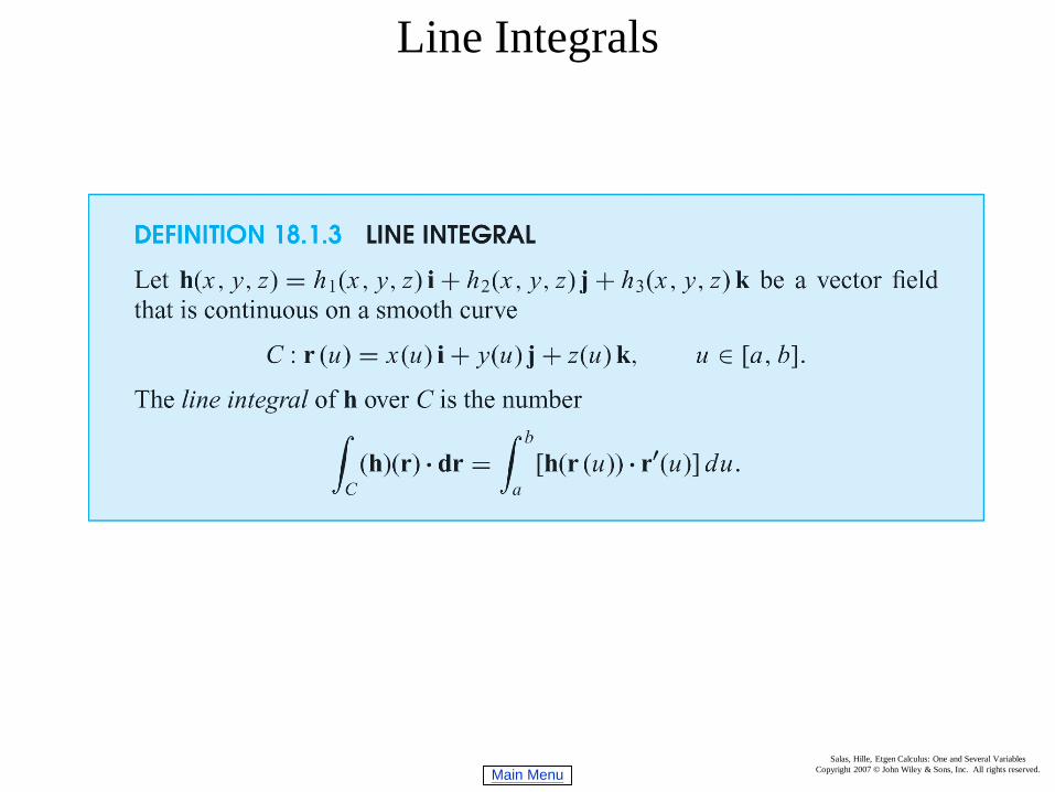
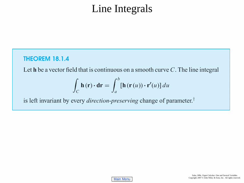
Section 18.1 Line Integralsa. Work Done by Varying Force Over a Curved Pathb. Definitionc. Theorem 18.1.4d. Piecewise Smoothnesse. Properties of Piecewise Smooth Curves
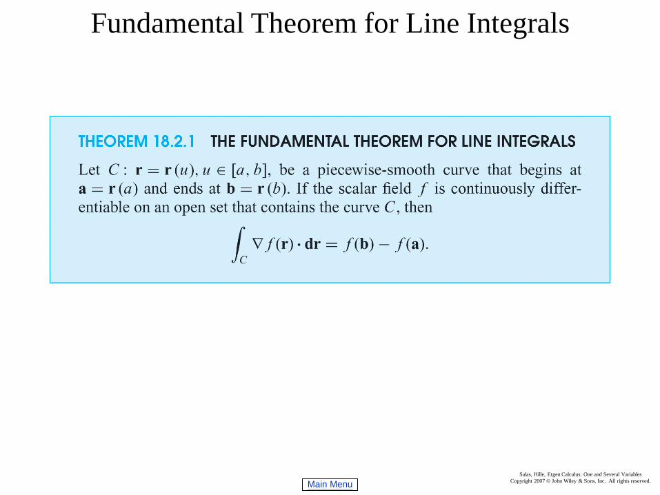
Section 18.2 Fundamental Theorem for Line Integralsa. Theorem 18.2.1b. Corollary and Example
Section 18.3 Work-Energy Formula; Conservation of Mechanical Energya. Work-Energy Formulab. Conservative Field, Potential Energy Functionsc. Conservation of Mechanical Energy
Section 18.4 Another Notation for Line Integrals; Line Integrals with Respect to Arc Lengtha. Line Integral with Respect to Arc Lengthb. Properties for a Thin Wire
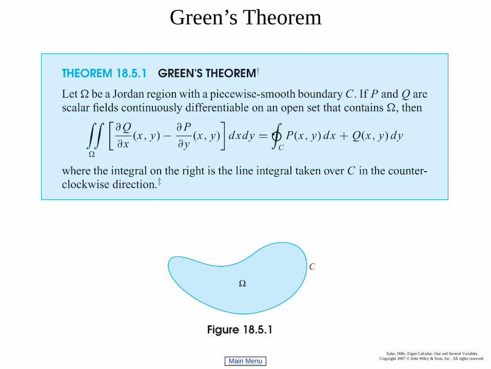
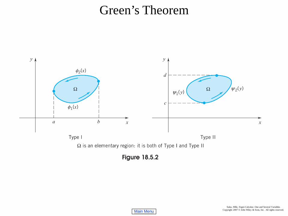
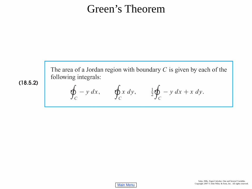
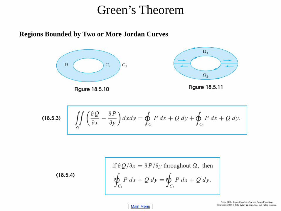
Section 18.5 Green’s Theorema. Green’s Theorem, Theorem 18.5.1b. Type I and Type II Regionc. Area of a Jordan Regiond. Regions Bounded by Two or More Jordan Curves
Section 18.6 Parametrized Surfaces; Surface Areaa. Parametrized Surfacesb. Fundamental Vector Product - Illustrationc. Fundamental Vector Product - Notationd. Area of a Parametrized Surfacee. Area of a Smooth Surfacef. Area of Surface z = f (x,y)
Chapter 18: Line Integrals and Surface IntegralsSection 18.7 Surface Integralsa. Mass of a Material Surfaceb. Surface Integralsc. Average Value of H on Sd. Moment of Inertiae. Flux of a Vector Field
Section 18.8 The Vector Differential Operator ∇a. Vector Differential Operatorb. Divergencec. Curld. Theorems for Divergence and Curle. Identities and Propertiesf. The Laplacian
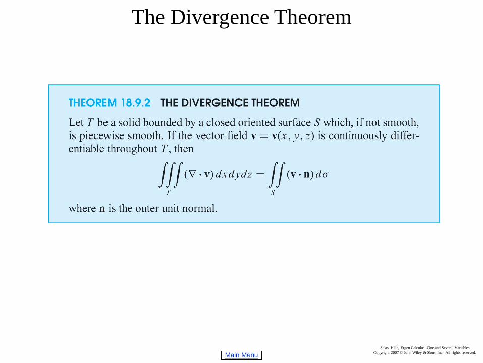
Section 18.9 The Divergence Theorema. Theorem 18.9.2b. Divergence as Outward Flux per Unit Volumec. Solids Bounded by Two or More Closed Surfaces
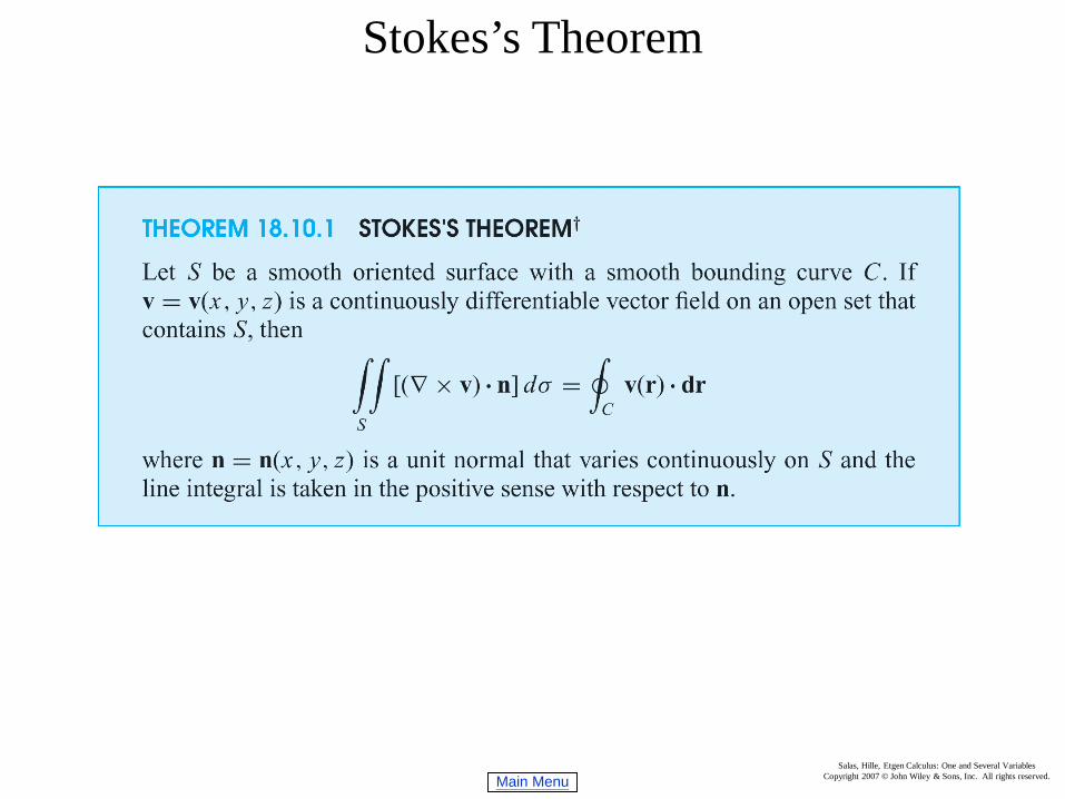
Section 18.10 Stokes’s Theorema. Theorem 18.10.1, Stokes’s Theoremb. Partial Converse to Stokes Theoremc. Irrotational Flowd. Theorem 18.10.3
Main MenuSalas, Hille, Etgen Calculus: One and Several Variables
Copyright 2007 © John Wiley & Sons, Inc. All rights reserved.
Line Integrals
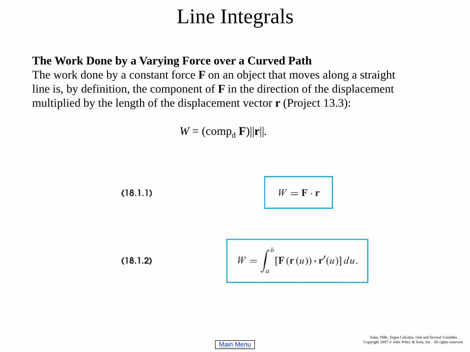
The Work Done by a Varying Force over a Curved PathThe work done by a constant force F on an object that moves along a straight line is, by definition, the component of F in the direction of the displacement multiplied by the length of the displacement vector r (Project 13.3):
W = (compd F)||r||.
Main MenuSalas, Hille, Etgen Calculus: One and Several Variables
Copyright 2007 © John Wiley & Sons, Inc. All rights reserved.
Line Integrals
Main MenuSalas, Hille, Etgen Calculus: One and Several Variables
Copyright 2007 © John Wiley & Sons, Inc. All rights reserved.
Line Integrals
Main MenuSalas, Hille, Etgen Calculus: One and Several Variables
Copyright 2007 © John Wiley & Sons, Inc. All rights reserved.
Line Integrals
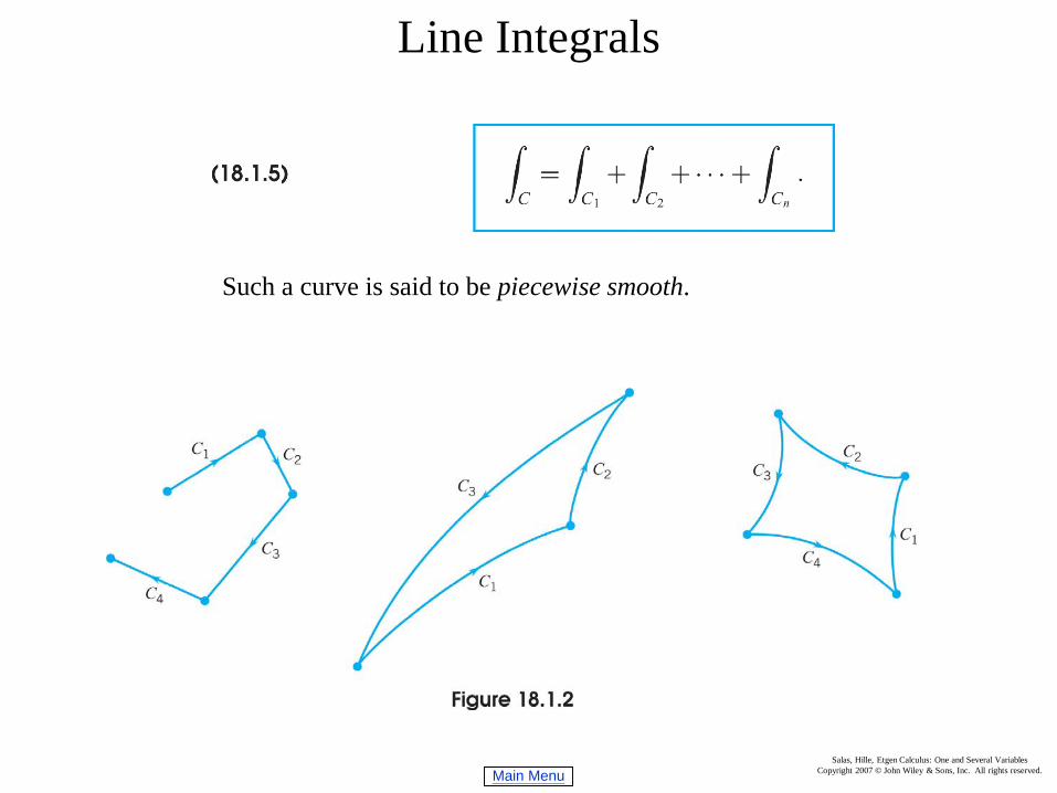
Such a curve is said to be piecewise smooth.
Main MenuSalas, Hille, Etgen Calculus: One and Several Variables
Copyright 2007 © John Wiley & Sons, Inc. All rights reserved.
Line Integrals
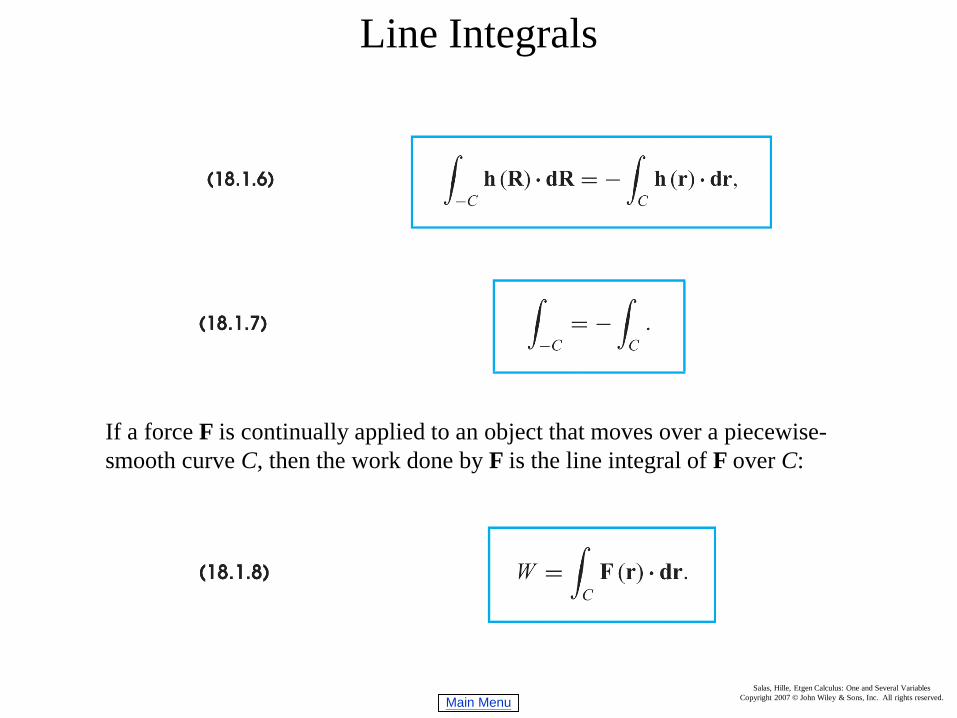
If a force F is continually applied to an object that moves over a piecewise-smooth curve C, then the work done by F is the line integral of F over C:
Main MenuSalas, Hille, Etgen Calculus: One and Several Variables
Copyright 2007 © John Wiley & Sons, Inc. All rights reserved.
Fundamental Theorem for Line Integrals
Main MenuSalas, Hille, Etgen Calculus: One and Several Variables
Copyright 2007 © John Wiley & Sons, Inc. All rights reserved.
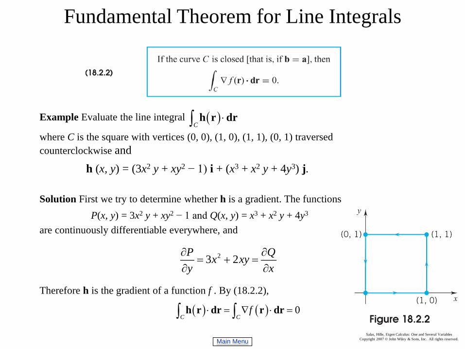
Fundamental Theorem for Line Integrals
Example Evaluate the line integral
where C is the square with vertices (0, 0), (1, 0), (1, 1), (0, 1) traversed counterclockwise and
h (x, y) = (3x2 y + xy2 − 1) i + (x3 + x2 y + 4y3) j.
Solution First we try to determine whether h is a gradient. The functionsP(x, y) = 3x2 y + xy2 − 1 and Q(x, y) = x3 + x2 y + 4y3
are continuously differentiable everywhere, and
Therefore h is the gradient of a function f . By (18.2.2),
( )C
⋅∫ h r dr
( ) ( ) 0C C
f⋅ = ∇ ⋅ =∫ ∫h r dr r dr
23 2P Qx xyy x
∂ ∂= + =
∂ ∂
Main MenuSalas, Hille, Etgen Calculus: One and Several Variables
Copyright 2007 © John Wiley & Sons, Inc. All rights reserved.
Work-Energy Formula; Conservation of Mechanical Energy
This relation is called the work–energy formula.
Main MenuSalas, Hille, Etgen Calculus: One and Several Variables
Copyright 2007 © John Wiley & Sons, Inc. All rights reserved.
Work-Energy Formula; Conservation of Mechanical Energy
Conservative Force FieldsIn general, if an object moves from one point to another, the work done (and hencethe change in kinetic energy) depends on the path of the motion. There is, however, an important exception: if the force field is a gradient field,
then the work done (and hence the change in kinetic energy) depends only on theendpoints of the path, not on the path itself. (This follows directly from the fundamental theorem for line integrals.) A force field that is a gradient field is called a conservative field.Since the line integral over a closed path is zero, the work done by a conservativefield over a closed path is always zero. An object that passes through a given point with a certain kinetic energy returns to that same point with exactly the same kinetic energy.
f= ∇F
Potential Energy FunctionsSuppose that F is a conservative force field. It is then a gradient field. Then −F isalso a gradient field. The functions U for which are called potential energy functions for F.
U∇ = −F
Main MenuSalas, Hille, Etgen Calculus: One and Several Variables
Copyright 2007 © John Wiley & Sons, Inc. All rights reserved.
Work-Energy Formula; Conservation of Mechanical Energy
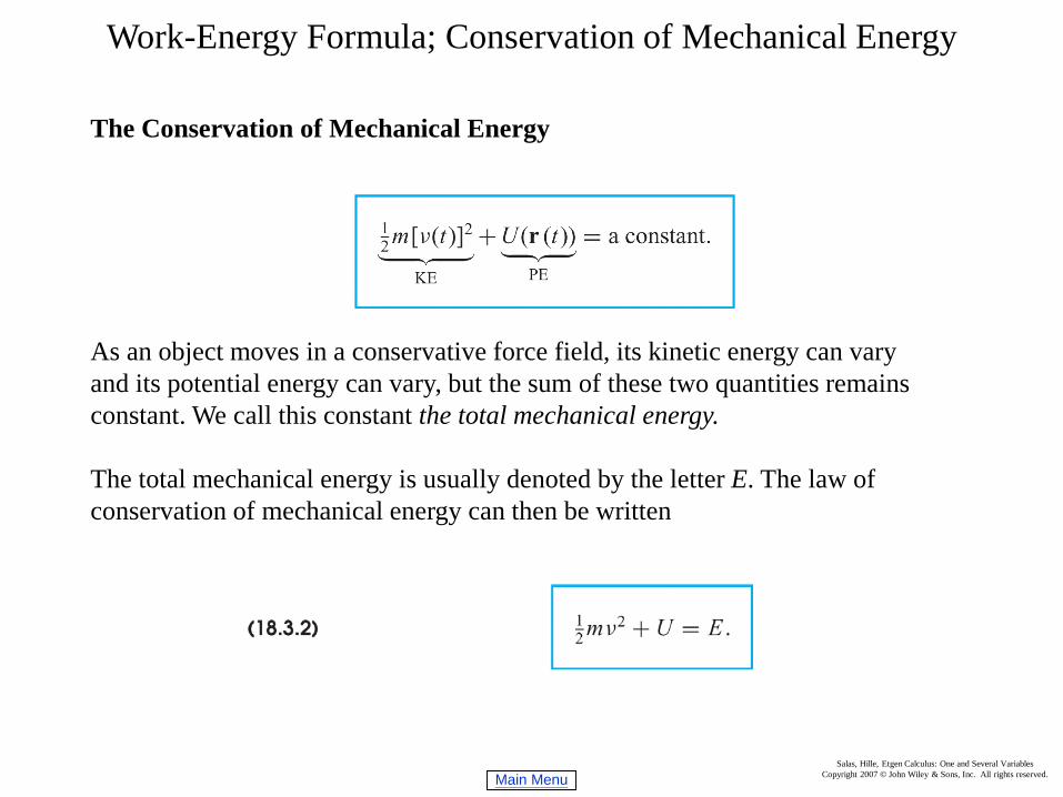
The Conservation of Mechanical Energy
As an object moves in a conservative force field, its kinetic energy can vary and its potential energy can vary, but the sum of these two quantities remains constant. We call this constant the total mechanical energy.
The total mechanical energy is usually denoted by the letter E. The law of conservation of mechanical energy can then be written
Main MenuSalas, Hille, Etgen Calculus: One and Several Variables
Copyright 2007 © John Wiley & Sons, Inc. All rights reserved.
Line Integrals with Respect to Arc Length
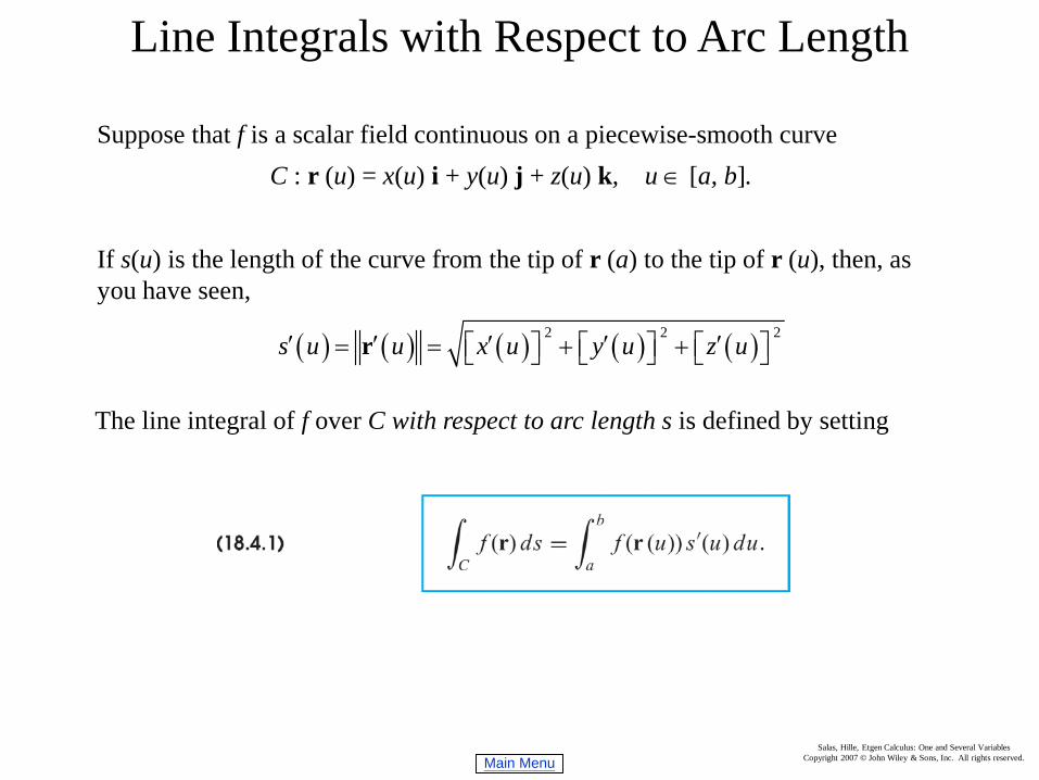
Suppose that f is a scalar field continuous on a piecewise-smooth curveC : r (u) = x(u) i + y(u) j + z(u) k, u ∈ [a, b].
If s(u) is the length of the curve from the tip of r (a) to the tip of r (u), then, as you have seen,
The line integral of f over C with respect to arc length s is defined by setting
( ) ( ) ( ) ( ) ( )2 2 2s u u x u y u z u′ ′ ′ ′ ′= = + + r
Main MenuSalas, Hille, Etgen Calculus: One and Several Variables
Copyright 2007 © John Wiley & Sons, Inc. All rights reserved.
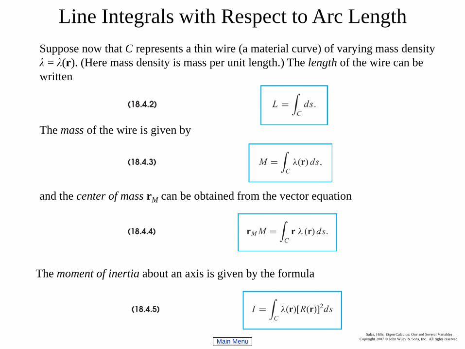
Line Integrals with Respect to Arc LengthSuppose now that C represents a thin wire (a material curve) of varying mass density λ = λ(r). (Here mass density is mass per unit length.) The length of the wire can be written
The mass of the wire is given by
and the center of mass rM can be obtained from the vector equation
The moment of inertia about an axis is given by the formula
Main MenuSalas, Hille, Etgen Calculus: One and Several Variables
Copyright 2007 © John Wiley & Sons, Inc. All rights reserved.
Green’s Theorem
Main MenuSalas, Hille, Etgen Calculus: One and Several Variables
Copyright 2007 © John Wiley & Sons, Inc. All rights reserved.
Green’s Theorem
Main MenuSalas, Hille, Etgen Calculus: One and Several Variables
Copyright 2007 © John Wiley & Sons, Inc. All rights reserved.
Green’s Theorem
Main MenuSalas, Hille, Etgen Calculus: One and Several Variables
Copyright 2007 © John Wiley & Sons, Inc. All rights reserved.
Green’s Theorem
Regions Bounded by Two or More Jordan Curves
Main MenuSalas, Hille, Etgen Calculus: One and Several Variables
Copyright 2007 © John Wiley & Sons, Inc. All rights reserved.
Parametrized Surfaces; Surface Area
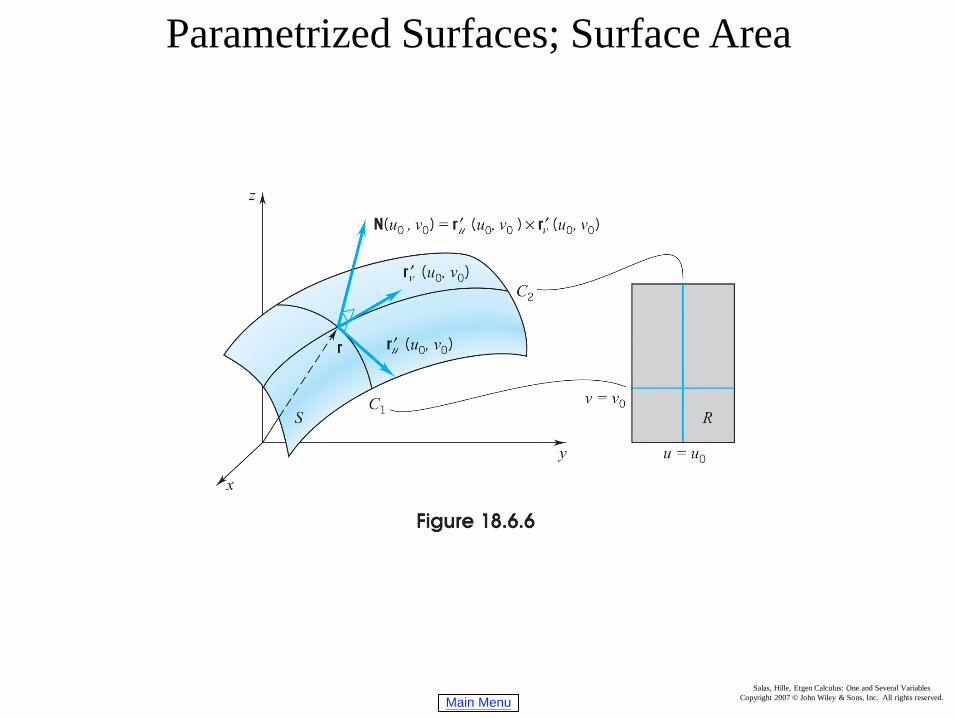
Main MenuSalas, Hille, Etgen Calculus: One and Several Variables
Copyright 2007 © John Wiley & Sons, Inc. All rights reserved.
Parametrized Surfaces; Surface Area
Main MenuSalas, Hille, Etgen Calculus: One and Several Variables
Copyright 2007 © John Wiley & Sons, Inc. All rights reserved.
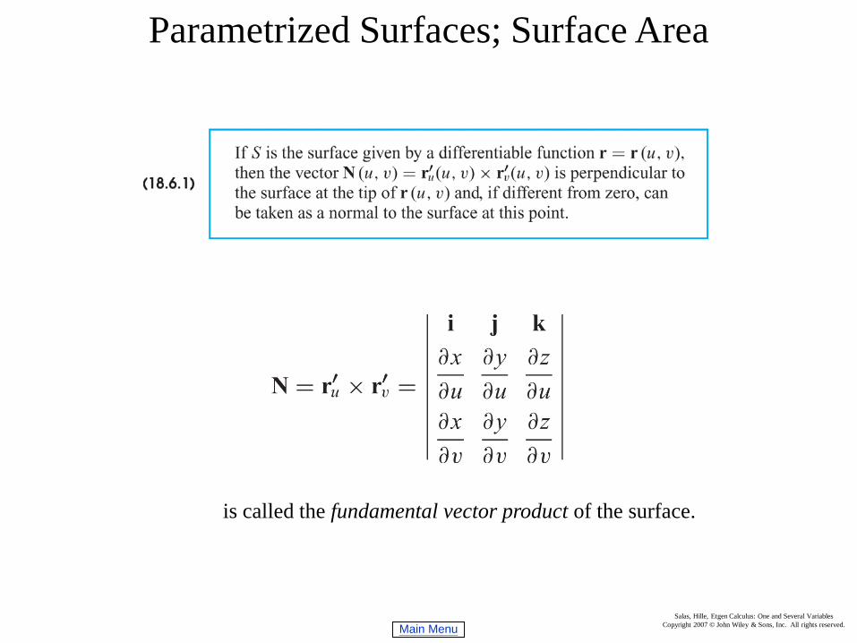
Parametrized Surfaces; Surface Area
is called the fundamental vector product of the surface.
Main MenuSalas, Hille, Etgen Calculus: One and Several Variables
Copyright 2007 © John Wiley & Sons, Inc. All rights reserved.
Parametrized Surfaces; Surface Area
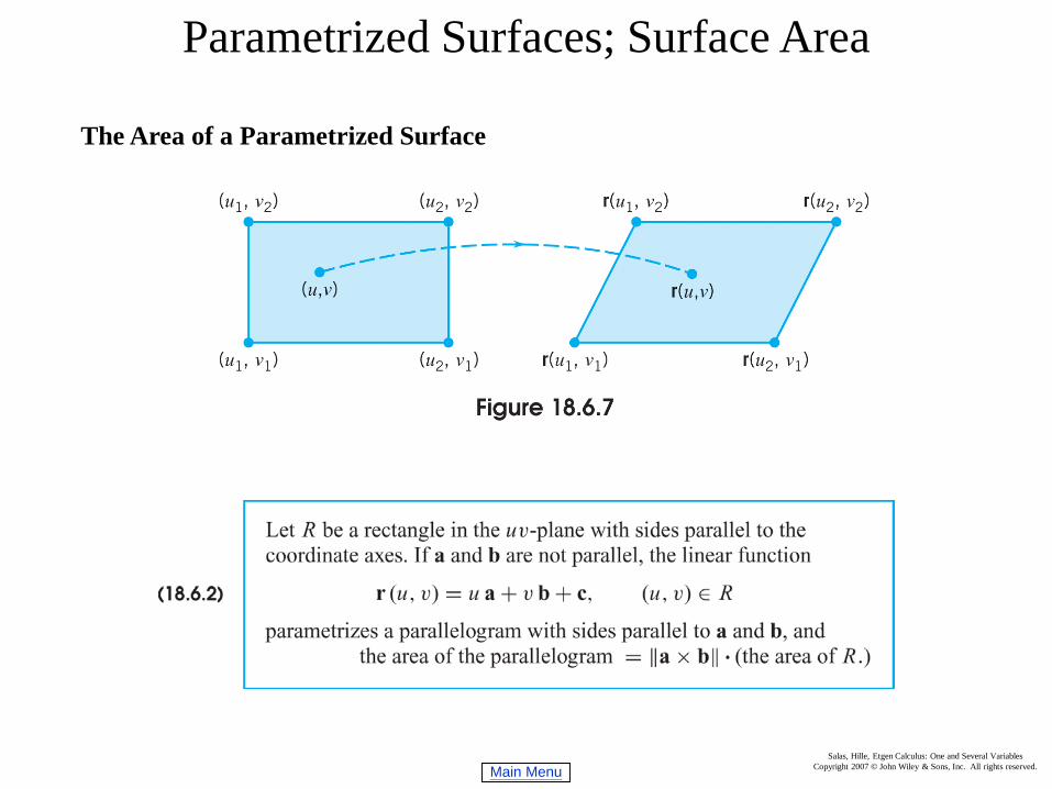
The Area of a Parametrized Surface
Main MenuSalas, Hille, Etgen Calculus: One and Several Variables
Copyright 2007 © John Wiley & Sons, Inc. All rights reserved.
Parametrized Surfaces; Surface Area
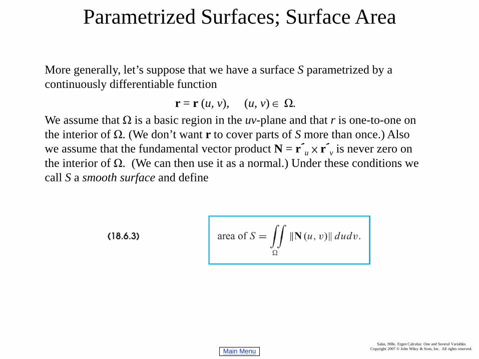
More generally, let’s suppose that we have a surface S parametrized by a continuously differentiable function
r = r (u, v), (u, v) ∈ Ω.We assume that Ω is a basic region in the uv-plane and that r is one-to-one on the interior of Ω. (We don’t want r to cover parts of S more than once.) Also we assume that the fundamental vector product N = r´u × r´v is never zero on the interior of Ω. (We can then use it as a normal.) Under these conditions we call S a smooth surface and define
Main MenuSalas, Hille, Etgen Calculus: One and Several Variables
Copyright 2007 © John Wiley & Sons, Inc. All rights reserved.
Parametrized Surfaces; Surface Area
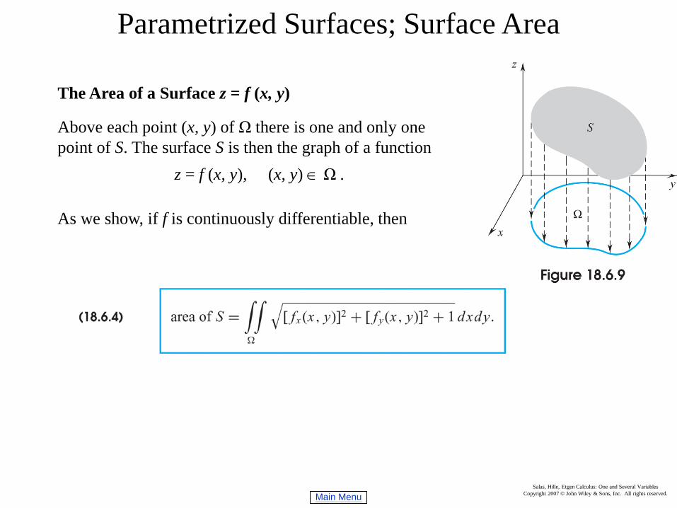
The Area of a Surface z = f (x, y)
Above each point (x, y) of Ω there is one and only one point of S. The surface S is then the graph of a function
z = f (x, y), (x, y) ∈ Ω .
As we show, if f is continuously differentiable, then
Main MenuSalas, Hille, Etgen Calculus: One and Several Variables
Copyright 2007 © John Wiley & Sons, Inc. All rights reserved.
Surface Integrals
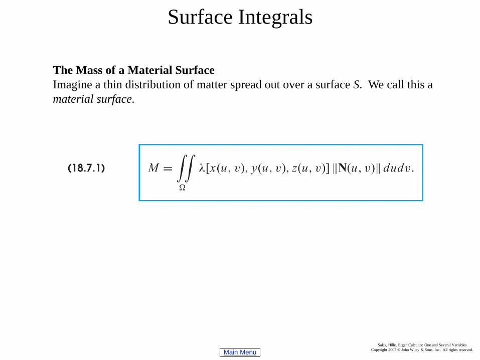
The Mass of a Material SurfaceImagine a thin distribution of matter spread out over a surface S. We call this a material surface.
Main MenuSalas, Hille, Etgen Calculus: One and Several Variables
Copyright 2007 © John Wiley & Sons, Inc. All rights reserved.
Surface Integrals
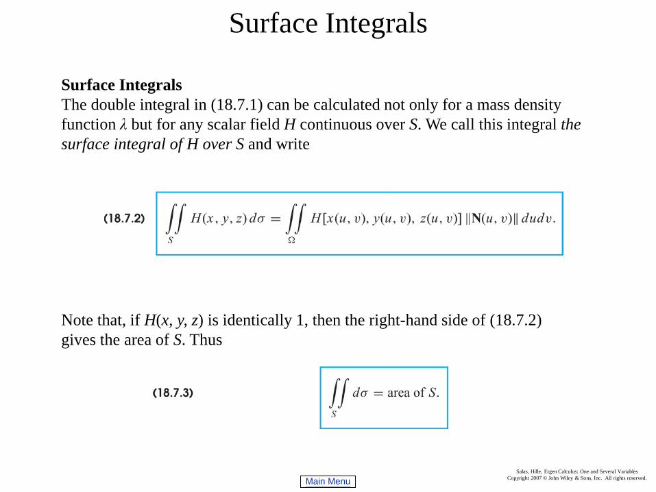
Surface IntegralsThe double integral in (18.7.1) can be calculated not only for a mass density function λ but for any scalar field H continuous over S. We call this integral the surface integral of H over S and write
Note that, if H(x, y, z) is identically 1, then the right-hand side of (18.7.2) gives the area of S. Thus
Main MenuSalas, Hille, Etgen Calculus: One and Several Variables
Copyright 2007 © John Wiley & Sons, Inc. All rights reserved.
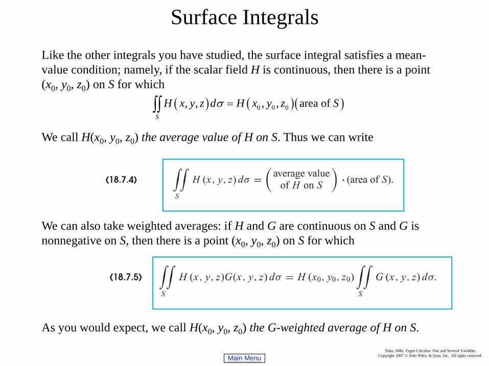
Surface IntegralsLike the other integrals you have studied, the surface integral satisfies a mean-value condition; namely, if the scalar field H is continuous, then there is a point (x0, y0, z0) on S for which
We call H(x0, y0, z0) the average value of H on S. Thus we can write
We can also take weighted averages: if H and G are continuous on S and G is nonnegative on S, then there is a point (x0, y0, z0) on S for which
As you would expect, we call H(x0, y0, z0) the G-weighted average of H on S.
( ) ( )( )0 0 0, , , , area of S
H x y z d H x y z Sσ =∫∫
Main MenuSalas, Hille, Etgen Calculus: One and Several Variables
Copyright 2007 © John Wiley & Sons, Inc. All rights reserved.
Surface Integrals
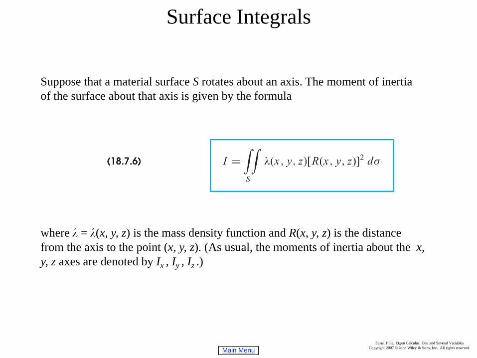
Suppose that a material surface S rotates about an axis. The moment of inertia of the surface about that axis is given by the formula
where λ = λ(x, y, z) is the mass density function and R(x, y, z) is the distance from the axis to the point (x, y, z). (As usual, the moments of inertia about the x, y, z axes are denoted by Ix , Iy , Iz .)
Main MenuSalas, Hille, Etgen Calculus: One and Several Variables
Copyright 2007 © John Wiley & Sons, Inc. All rights reserved.
Surface Integrals
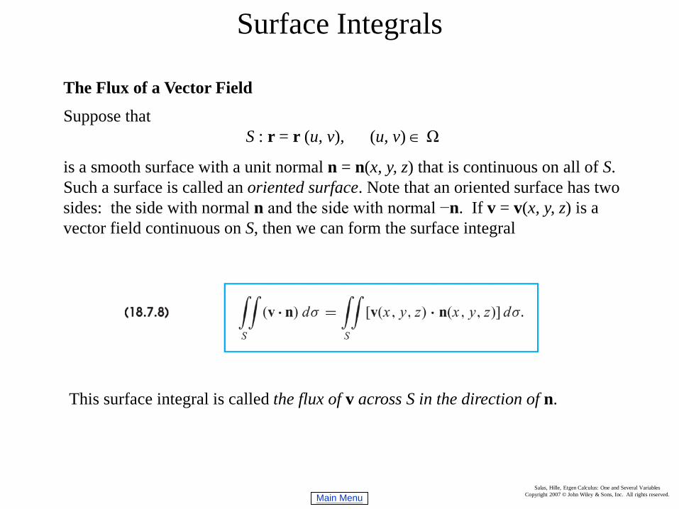
The Flux of a Vector Field
Suppose thatS : r = r (u, v), (u, v) ∈ Ω
is a smooth surface with a unit normal n = n(x, y, z) that is continuous on all of S. Such a surface is called an oriented surface. Note that an oriented surface has two sides: the side with normal n and the side with normal −n. If v = v(x, y, z) is a vector field continuous on S, then we can form the surface integral
This surface integral is called the flux of v across S in the direction of n.
Main MenuSalas, Hille, Etgen Calculus: One and Several Variables
Copyright 2007 © John Wiley & Sons, Inc. All rights reserved.
The Vector Differential Operator
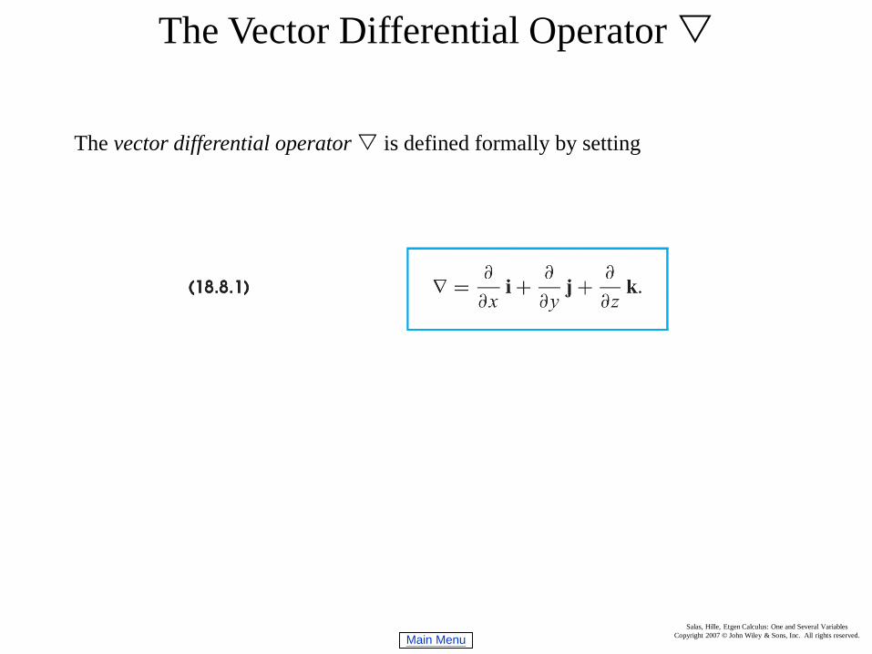
The vector differential operator is defined formally by setting
Main MenuSalas, Hille, Etgen Calculus: One and Several Variables
Copyright 2007 © John Wiley & Sons, Inc. All rights reserved.
The Vector Differential Operator
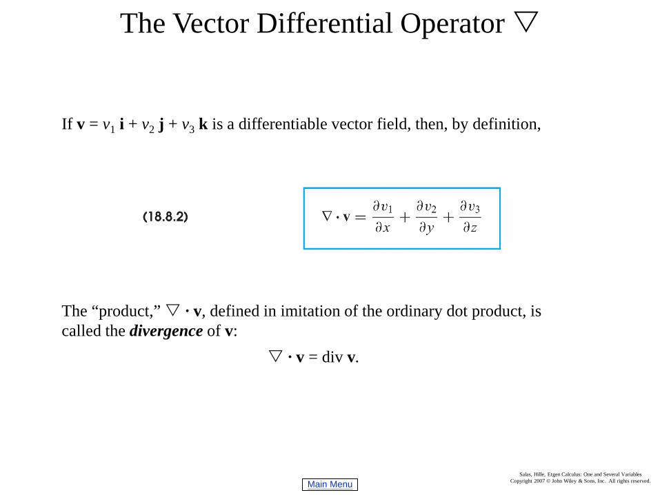
If v = v1 i + v2 j + v3 k is a differentiable vector field, then, by definition,
The “product,” · v, defined in imitation of the ordinary dot product, is called the divergence of v:
· v = div v.
Main MenuSalas, Hille, Etgen Calculus: One and Several Variables
Copyright 2007 © John Wiley & Sons, Inc. All rights reserved.
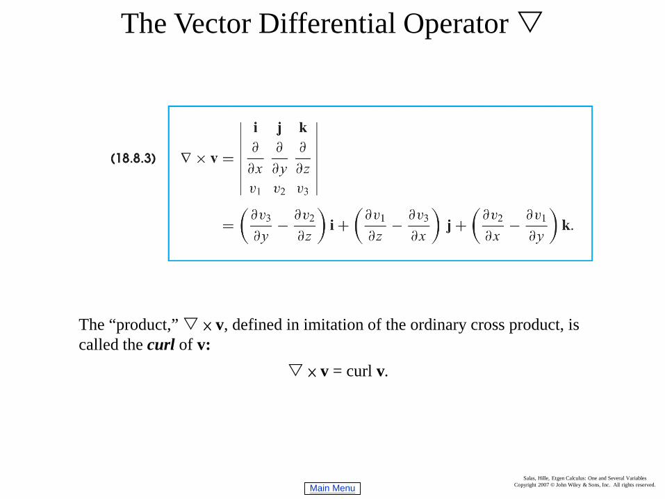
The Vector Differential Operator
The “product,” × v, defined in imitation of the ordinary cross product, is called the curl of v:
× v = curl v.
Main MenuSalas, Hille, Etgen Calculus: One and Several Variables
Copyright 2007 © John Wiley & Sons, Inc. All rights reserved.
The Vector Differential Operator
Main MenuSalas, Hille, Etgen Calculus: One and Several Variables
Copyright 2007 © John Wiley & Sons, Inc. All rights reserved.
The Vector Differential Operator
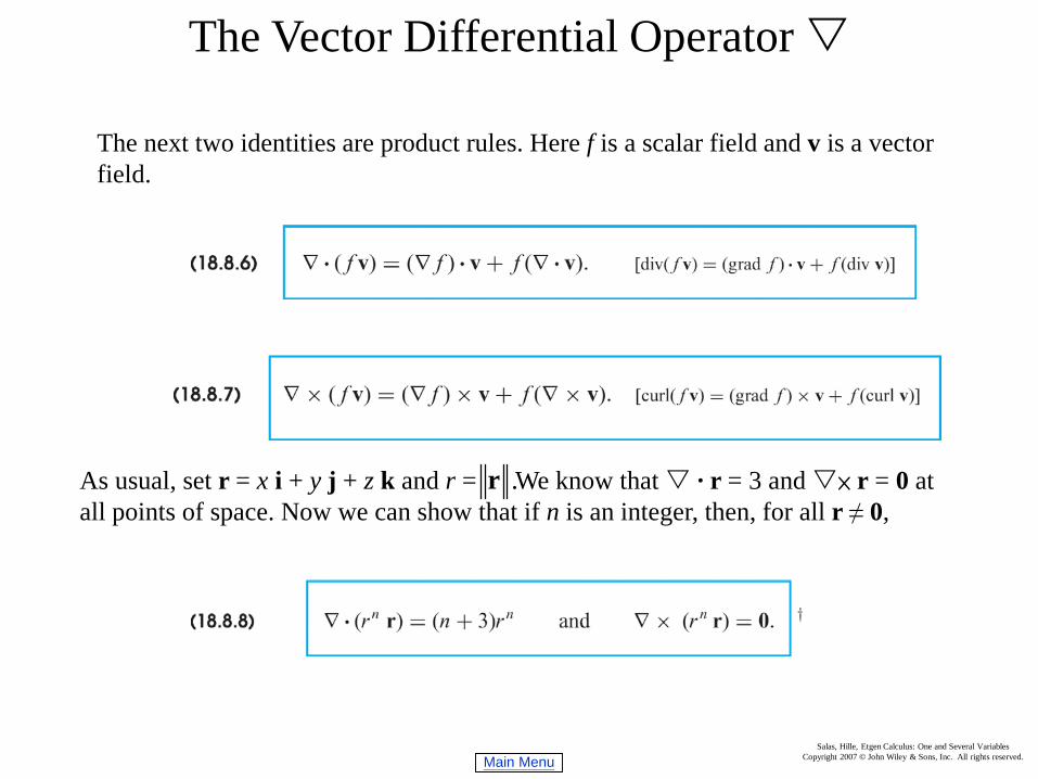
The next two identities are product rules. Here f is a scalar field and v is a vectorfield.
As usual, set r = x i + y j + z k and r = We know that · r = 3 and × r = 0 at all points of space. Now we can show that if n is an integer, then, for all r ≠ 0,
.r
Main MenuSalas, Hille, Etgen Calculus: One and Several Variables
Copyright 2007 © John Wiley & Sons, Inc. All rights reserved.
The Vector Differential Operator
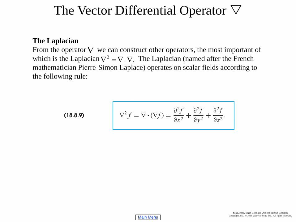
The LaplacianFrom the operator we can construct other operators, the most important of which is the Laplacian The Laplacian (named after the French mathematician Pierre-Simon Laplace) operates on scalar fields according to the following rule:
∇2 .∇ =∇⋅∇
Main MenuSalas, Hille, Etgen Calculus: One and Several Variables
Copyright 2007 © John Wiley & Sons, Inc. All rights reserved.
The Divergence Theorem
Main MenuSalas, Hille, Etgen Calculus: One and Several Variables
Copyright 2007 © John Wiley & Sons, Inc. All rights reserved.
The Divergence Theorem
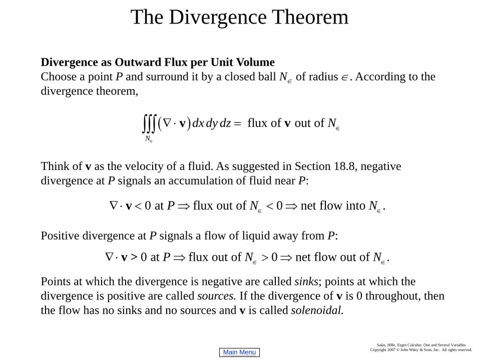
Divergence as Outward Flux per Unit VolumeChoose a point P and surround it by a closed ball N∈ of radius ∈. According to thedivergence theorem,
Think of v as the velocity of a fluid. As suggested in Section 18.8, negative divergence at P signals an accumulation of fluid near P:
Positive divergence at P signals a flow of liquid away from P:
Points at which the divergence is negative are called sinks; points at which the divergence is positive are called sources. If the divergence of v is 0 throughout, then the flow has no sinks and no sources and v is called solenoidal.
( ) flux of out of N
dx dy dz N∈
∈∇ ⋅ =∫∫∫ v v
0 at flux out of 0 net flow into .P N N∈ ∈∇ ⋅ < ⇒ < ⇒v
0 at flux out of 0 net flow out of .P N N∈ ∈∇ ⋅ ⇒ > ⇒v >
Main MenuSalas, Hille, Etgen Calculus: One and Several Variables
Copyright 2007 © John Wiley & Sons, Inc. All rights reserved.
The Divergence Theorem
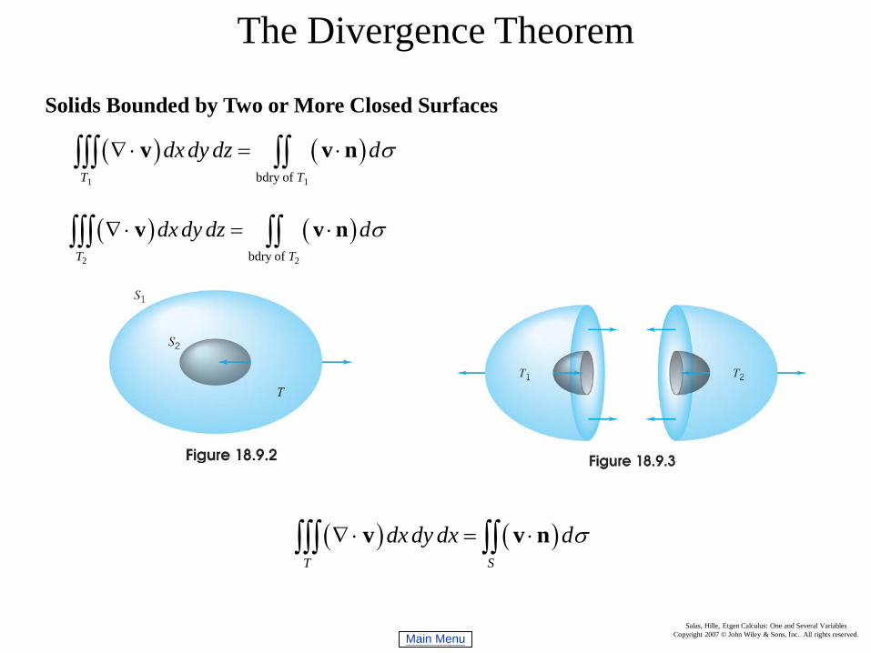
Solids Bounded by Two or More Closed Surfaces
( ) ( )1 1bdry of T T
dx dy dz dσ∇ ⋅ = ⋅∫∫∫ ∫∫v v n
( ) ( )2 2bdry of T T
dx dy dz dσ∇ ⋅ = ⋅∫∫∫ ∫∫v v n
( ) ( )T S
dx dy dx dσ∇ ⋅ = ⋅∫∫∫ ∫∫v v n
Main MenuSalas, Hille, Etgen Calculus: One and Several Variables
Copyright 2007 © John Wiley & Sons, Inc. All rights reserved.
Stokes’s Theorem
Main MenuSalas, Hille, Etgen Calculus: One and Several Variables
Copyright 2007 © John Wiley & Sons, Inc. All rights reserved.
Stokes’s Theorem
Main MenuSalas, Hille, Etgen Calculus: One and Several Variables
Copyright 2007 © John Wiley & Sons, Inc. All rights reserved.
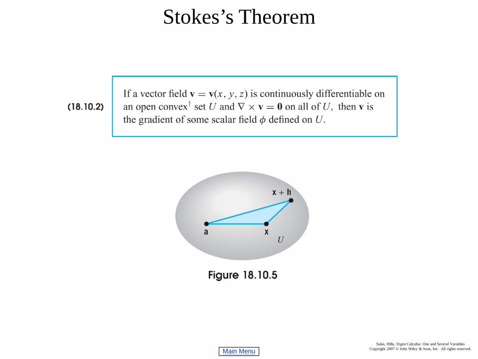
Stokes’s Theorem
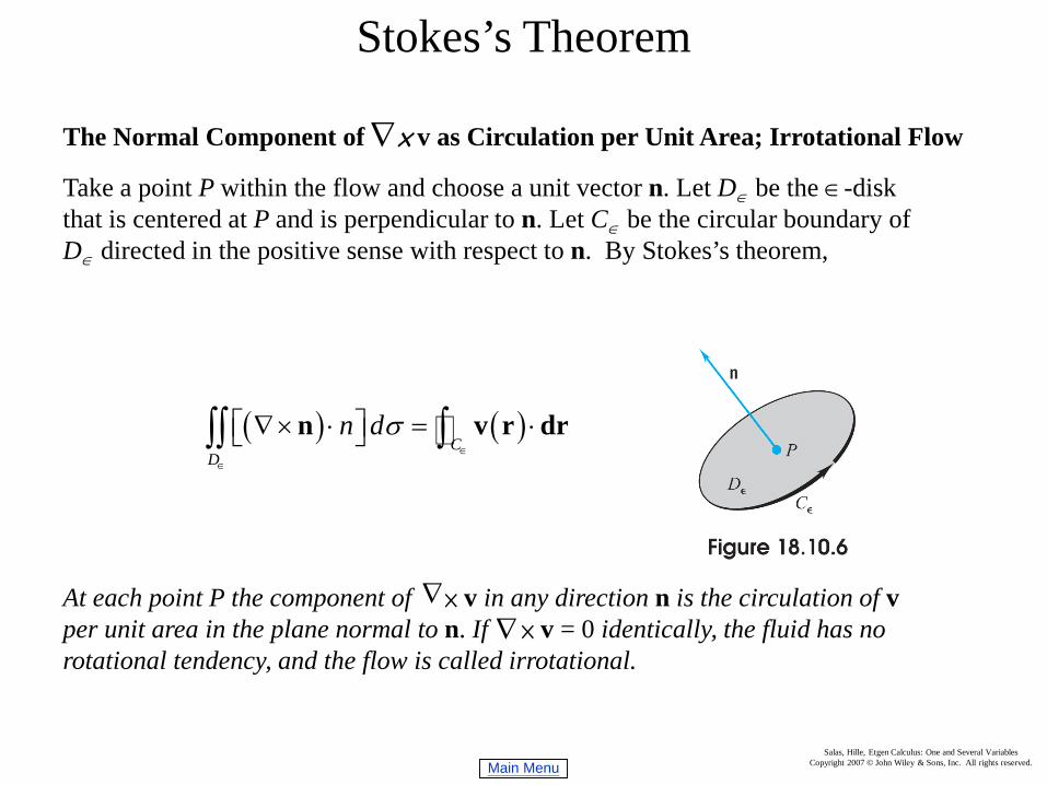
The Normal Component of × v as Circulation per Unit Area; Irrotational Flow
Take a point P within the flow and choose a unit vector n. Let D∈ be the ∈-diskthat is centered at P and is perpendicular to n. Let C∈ be the circular boundary ofD∈ directed in the positive sense with respect to n. By Stokes’s theorem,
( ) ( )C
D
n dσ∈
∈
∇× ⋅ = ⋅ ∫∫ ∫n v r dr
At each point P the component of × v in any direction n is the circulation of v per unit area in the plane normal to n. If × v = 0 identically, the fluid has no rotational tendency, and the flow is called irrotational.
∇
∇∇
Main MenuSalas, Hille, Etgen Calculus: One and Several Variables
Copyright 2007 © John Wiley & Sons, Inc. All rights reserved.
Stokes’s Theorem