Line Integrals - University of California, Berkeleywodzicki/H185.S11/podrecznik/li.pdf · Line Integrals October 23, 2003 ... 1Abbreviation DCVF stands for Differential Calculus of

Math 53M, Fall 2003 Professor Mariusz Wodzicki

Line IntegralsOctober 23, 2003

These notes should be studied in conjunction with lectures.1

1 Path integrals Let γ : [a,b] → Rm be a path contained in a subset D ⊆ Rm and let

ϕ : D× Rm → R (1)

be a function of two variables: a point x ∈ D and a column-vector v ∈ Rm .

We shall define the integral∫

γ

ϕ as the limit

∫γ

ϕ ˜ lim|P|→0

k∑j=1

ϕ(γ(t∗j ); γ(tj) − γ(tj−1)) (2)

where the limit is taken over all tagged partitions P of interval [a,b]:

a = t0 < t1 < · · · < tk = b (t∗j ∈ [tj−1, tj]) (3)

while the mesh of the partition

|P |˜max(|t1 − t0|, . . . , |tk − tk−1|) (4)

tends to zero. Limit (2), when exists, is called the integral of ϕ along path γ. L2 An alternative approach For functions whose arguments are vectors anchored at pointsof D,

φ :{−→ab

∣∣ a ∈ D}→ R , (5)

the definition of integral∫

γ

φ is more natural:

1Abbreviation DCVF stands for Differential Calculus of Vector Functions.

1


∫γ

φ ˜ lim|P|→0

k∑j=1

φ(−−−→aj−1aj) (6)

where the limit in (6) is taken over all (not tagged) partitions of interval [a,b]:

a = t0 < t1 < · · · < tk = b , (7)

and aj˜ γ(tj). Isn’t definition (6) also simpler than (2)?

a

a

a

a

a

k−1

k

2

1

0

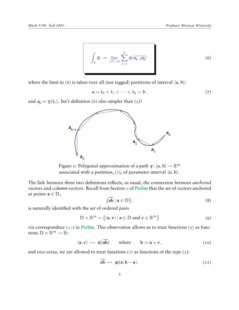
Figure 1: Polygonal approximation of a path γ : [a,b] → Rm

associated with a partition, (7), of parameter interval [a,b].

The link between these two definitions reflects, as usual, the connection between anchoredvectors and column-vectors. Recall from Section 9 of Prelim that the set of vectors anchoredat points a ∈ D, {−→

ab | a ∈ D}

, (8)

is naturally identified with the set of ordered pairs

D× Rm ={(a, v) | a ∈ D and v ∈ Rm

}(9)

via correspondnce (23) in Prelim. This observation allows us to treat functions (5) as func-tions D× Rm → R :

(a, v) 7→ φ(−→ab) where b˜ a + v , (10)

and vice-versa, we are allowed to treat functions (1) as functions of the type (5):

−→ab 7→ ϕ(a; b − a) . (11)

2


Having these identifications in mind, one now sees that definition of path integral (6) cor-responds to definition (2), if one tags each partition P at the left ends of subintervals[tj−1, tj]:

t∗j ˜ tj−1 (12)

for all 0 6 j 6 k.

3 Basic properties Two fundamental properties of path integral follow directly from itsdefinition:

additivity with respect to integrand∫γ

(ϕ +ψ) =

∫γ

ϕ +

∫γ

ψ (13)

and

additivity with respect to path ∫γ1t γ2

ϕ =

∫γ1

ϕ +

∫γ2

ϕ . (14)

Here γ1 is a path [a,b] → Rm , γ2 is a path [b, c] → Rm and the endpoint of γ1 is supposedto coincide with the beginning of γ2 :

γ1(b) = γ2(b) . (15)

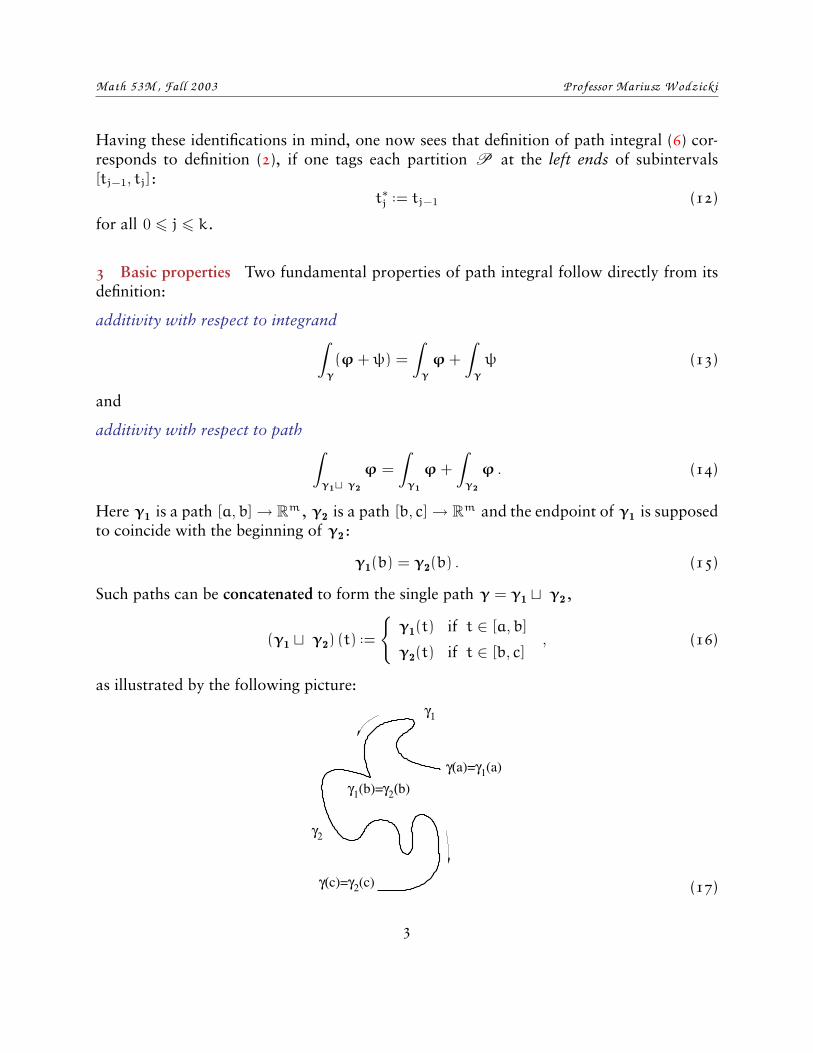
Such paths can be concatenated to form the single path γ = γ1 t γ2 ,

(γ1 t γ2) (t)˜

{γ1(t) if t ∈ [a,b]

γ2(t) if t ∈ [b, c], (16)

as illustrated by the following picture:

γ1(b)=γ2(b)

γ(c)=γ2(c)

γγ(a)= (a)1

γ2

γ1

(17)

3


4 Path length The function λ : Rm × Rm → R :

λ(a; v)˜ ‖v‖ (the norm of v) (18)

corresponds to the function associating with a vector−→ab its length ‖b − a‖. In particular,

(18) does not depend on a point a; it depends only on v . For any path γ, the integral

Length(γ)˜

∫γ

λ (19)

exists in the sense that it is either finite:

Length(γ) < ,

in this case we say that γ is a rectifiable path, orRLength(γ) = ,

in which case we say that path γ is nonrectifiable.RThis follows from the fact that

∫γ

λ is the limit of lengths

k∑j=1

ww−−−→aj−1ajww (20)

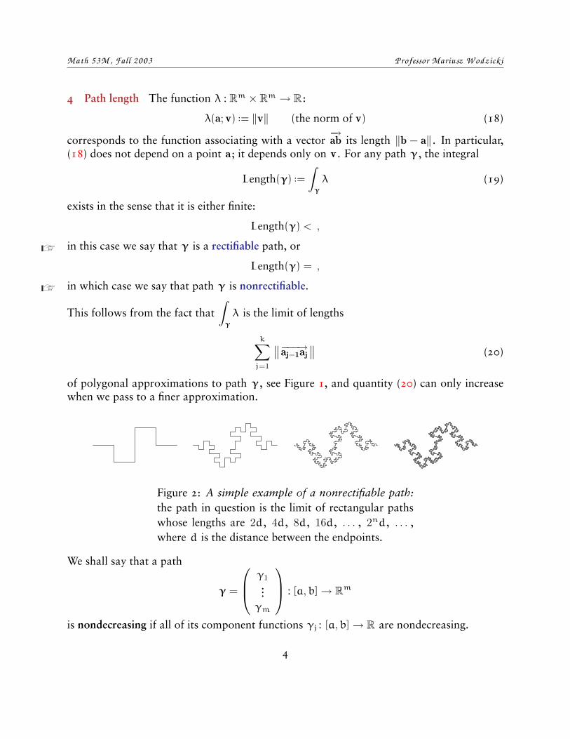
of polygonal approximations to path γ, see Figure 1, and quantity (20) can only increasewhen we pass to a finer approximation.

Figure 2: A simple example of a nonrectifiable path:the path in question is the limit of rectangular pathswhose lengths are 2d, 4d, 8d, 16d, . . . , 2nd, . . . ,where d is the distance between the endpoints.

We shall say that a path

γ =

γ1...γm

: [a,b] → Rm

is nondecreasing if all of its component functions γj : [a,b] → R are nondecreasing.

4


5 Theorem Any nondecreasing path is rectifiable.

Indeed, for such a path, one has an obvious inequality

Length(γ) 6m∑

i=1

(γi(b) − γi(a)) < . (21)

W Exercise 1 Explain how to get inequality (21).

W Exercise 2 Show that:

(a) Length(γ1 + γ2) 6 Length(γ1) + Length(γ2) ,

(b) Length(cγ) = |c| Length(γ) .

It follows from the above exercise that a linear combination of rectifiable paths is rectifiable.In particular, the difference of two nondecreasing paths

γ = γ1 − γ2 (22)

is rectifiable.2 That the reverse is true is a remarkable theorem discovered by French math-ematician Marie Ennemond Camille Jordan (1838–1922).

6 Jordan’s Theorem3 A path γ is rectifiable if and only if it can be represented as differ-ence (22) of two nondecreasing paths.

7 Even everywhere differentiable paths need not be rectifiable, but general continuouspaths can be truly astounding. A theorem due to Polish mathematician Stefan Mazurkiewicz(1888–1945) and Austrian Hans Hahn (1879–1934) says that

Any subset S ⊆ Rm which is connected, locally connected4, closed,5

and bounded,6 is necessarily a continuous image of interval [0, 1].

2We define γ1 − γ2 by (γ1 − γ2)(t)˜ γ1(t) − γ1(t) .3Course d’analyse de l’École Polytechnique, 3 vols, Paris, 1882.4A set is locally connected if every point in it has an arbitrarily small connected neighborhood.5A set is closed if it contains all its accumulation points.6A set is bounded if it it is contained in some ball.

5

http://www-gap.dcs.st-and.ac.uk/~history/Mathematicians/Jordan.html

http://www-gap.dcs.st-and.ac.uk/~history/Mathematicians/Mazurkiewicz.html

http://www-gap.dcs.st-and.ac.uk/~history/Mathematicians/Hahn.html


The first example of such a path is the famous Peano curve,7 i.e. a continuous functionfrom [0, 1] onto the unit square in the plane. You can learn more about it by visiting thefollowing web sites:

go to: http://www.math.ohio-state.edu/~fiedorow/math655/Peano.html

go to: http://www.cut-the-knot.com/do_you_know/hilbert.shtml

go to: http://mmc.et.tudelft.nl/~frits/peanogrow.html

go to: http://www.csua.berkeley.edu/~raytrace/java/peano/peano.html

go to: http://www-math.uni-paderborn.de/~fazekas/course/peano.html

go to: http://www.geom.umn.edu/~dpvc/CVM/1998/01/vsfcf/article/sect8/peano.html

8 If f : D → R is a function on D then the integral of f along path γ is defined as the Lintegral ∫

γ

fλ (23)

where (fλ)(x; v) = f(x)‖v‖ . In Section 24 we shall find a method to calculate such integrals.

9 Differential forms Among all functions (1) those which are linear with respect to thecolumn-vector variable:

ϕ(x;av + bw) = aϕ(x; v) + bϕ(x; w) (a,b ∈ R; v, w ∈ Rm) (24)

play a particularly important role. They are called differential forms8 on set D ⊆ Rm .

W Exercise 3 Let f : D → R be a function and ϕ : D × Rm → R a differential form. Verifythat fϕ is a differential form.

For any differentiable function f : D→ R , its differential:

df : D× Rm → R, df(x; v)˜ (f ′(x))(v) (25)

(cf. DCVF, p. 17) is a differential form on D.

7Discovered in 1890 by Italian mathematician Giuseppe Peano (1858–1932).8Or, more precisely, differential 1-forms, since we are going to encounter later also 0 -forms, see Section

34, 2-forms and 3-forms.

6

http://www.math.ohio-state.edu/~fiedorow/math655/Peano.html

http://www.cut-the-knot.com/do_you_know/hilbert.shtml

http://mmc.et.tudelft.nl/~frits/peanogrow.html

http://www.csua.berkeley.edu/~raytrace/java/peano/peano.html

http://www-math.uni-paderborn.de/~fazekas/course/peano.html

http://www.geom.umn.edu/~dpvc/CVM/1998/01/vsfcf/article/sect8/peano.html

http://www-gap.dcs.st-and.ac.uk/~history/Mathematicians/Peano.html


It is customary to denote by dxi the differential of the i-th coordinate function πi : Rm →R :

πi

v1

...vm

˜ vi (26)

Forms dx1 , . . . , dxm are often called basic differential forms. One reason why are they Limportant is the following fact.

10 Proposition Every differential form ϕ on D ⊆ Rm can be expressed as

ϕ = f1dx1 + · · ·+ fmdxm (27)

for unique functions f1 , . . . , fm on D.

Indeed, for any vector v ∈ Rm , one has

v =

v1...vm

= v1e1 + · · ·+ vmem

and hence

ϕ(x; v) = ϕ(x; e1)v1 + · · ·+ ϕ(x; em)vm

= ϕ(x; e1)dx1(x; v) + · · ·+ ϕ(x; em)dxm(x; v) . (28)

Thus, if we introduce the functions

fi(x)˜ϕ(x; ei) , (29)

then identity (28) readsϕ = f1dx1 + · · ·+ fmdxm

as desired. To show the uniqueness of representation (27), note that

dxj(x; ei) =

{1 if j = i

0 if j 6= i. (30)

Hence,(f1dx1 + · · ·+ fmdxm)(x; ei) = fi(x)

which shows that the coefficient functions fi must be given by formula (29).

7


11 A differential form is said to be constant if its coefficient functions f1 , . . . , fm are Lconstant.

12 Identity (27) can be rewritten in abbreviated form as

ϕ = F · dx (31)

where F : D→ Rm is a function9 whose components are functions f1 , . . . , fm :

F˜

f1...fm

and dx : Rm × Rm → Rm is the vector valued form:

dx˜

dx1...

dxm

. (32)

W Exercise 4 What is dx(x; v) equal to?

W Exercise 5 What is F equal to when ϕ = df is the differential of a function f : D→ R ?

13 When College Multivariable Calculus textbooks10 talk about integrating a vector fieldF along a path γ what is meant by that is the integral∫

γ

F · dx =

∫γ

(f1dx1 + · · ·+ fmdxm) .

14 Riemann Integral as a special case of path integral You should have recognized bynow that the definite integral ∫ b

a

f(t)dt

9In College textbooks of Multivariable calculus such a function is often called a vector field on set D ⊆Rm .

10Or, oldfashioned textbooks of Physics.

8


from Freshman Calculus is the integral of fdt, considered as a differential form on intervalD = [a,b], along the path in R which traverses interval [a,b] with constant velocity 1 . Weshall denote this path by ι:11

ι : [a,b] → R , ι(t) = t . (33)

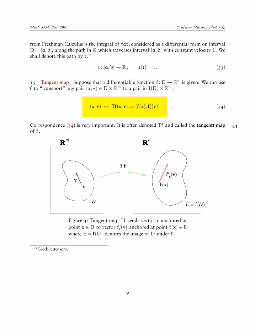
15 Tangent map Suppose that a differentiable function f : D→ Rn is given. We can usef to “transport” any pair (x; v) ∈ D× Rm to a pair in f(D)× Rn :

(x; v) 7→ T f(x; v)˜ (f(x); f ′x(v)) . (34)

Correspondence (34) is very important. It is often denoted Tf and called the tangentt map Lof f .

( )v

Rm

x

( )xv

x f

f’

fT

D

Rn

E = Df ( )

Figure 3: Tangent map T f sends vector v anchored atpoint x ∈ D to vector f ′x(v) anchored at point f(x) ∈ Ewhere E = f(D) denotes the image of D under f .

11Greek letter iota.

9


16 Pullback Denote by E = f(D) the subset of Rn which is the image of f . Given afunction ϕ : E×Rn → R , we can define a new function12 χ : D×Rm → R by the formula

χ(x; v)˜ (ϕ ◦ T f)(x; v) = ϕ(f(x); f ′x(v)) . (35)

W Exercise 6 Verify that χ is a differential form if ϕ is one.

Function χ is denoted f∗ϕ and called the pullback of ϕ by function f .

W Exercise 7 Verify the following properties of pullback:

(a) f∗(ϕ1 + ϕ2) = f∗ϕ1 + f∗ϕ2 and f∗(ϕ1ϕ2) = (f∗ϕ1) (f∗ϕ2);

(b) f∗ϕ = ϕ ◦ f if ϕ does not depend on the column-vector variable (i.e., if ϕ is simplya function E→ R);

(c) (f ◦ g)∗ϕ = g∗(f∗ϕ) . (Hint: Use the Chain Rule.)

17 Calculating pullbacks 1) On R we have constant differential form dt. If f : D → Ris a differentiable function then the calculation

(f∗(dt))(x; v) = dt(f(x); f ′x(v)) = f ′x(v) = df(x; v)

demonstrates thatf∗(dt) = df , (36)

i.e., the differential of f is the pullback, by f, of the standard differential form dt on R .

2) For a function g : E→ R and a vector-function f : D→ Rn whose image is contained inset E, one has

(f∗dg)(x; v) = dg(f(x)); f ′x(v)) = g ′f(x)(f′x(v)) = (g ′f(x) ◦ f ′x)(v)

which, by the Chain Rule, equals

(g ◦ f) ′x(v) = d(g ◦ f)(x; v) .12Greek letter khi.

10


In other words,f∗dg = d(g ◦ f) . (37)

Since fi = πi ◦ f and dxi = dπi , formula (37) yields the identity

f∗dxi = f∗dπi = (πi ◦ f)∗dt = dfi . (38)

3) Let ϕ = f1dx1 + · · ·+ fmdxm be a differential form on D ⊆ Rm , and γ : [a,b] → Rm bea path contained in D . In view of formula (38) we have

γ∗(f1dx1 + · · ·+ fmdxm) = (f1 ◦ γ) (γ∗dx1) + · · ·+ (fm ◦ γ) (γ∗dxm)

= (f1 ◦ γ)dγ1 + · · ·+ (fm ◦ γ)dγm

=

m∑i=1

(fi ◦ γ)dγi

dtdt =

((F ◦ γ) · dγ

dt

)dt (39)

4) Let x1 , . . . , xm be coordinates in Rm and y1 , . . . , yn be coordinates in Rn . For ageneral vector-function f : D→ Rn , one has

f∗(g1dy1 + · · ·+ gndyn) = (g1 ◦ f) f∗dy1 + · · ·+ (gn ◦ f) f∗dyn

= (g1 ◦ f)df1 + · · ·+ (gn ◦ f)dfn = (G ◦ f) · df (40)

where

G˜

g1...gn

and

df ˜

df1...

dfm

=

∂f1

∂xl

dx1 + · · ·+ ∂f1

∂xm

dxm

. . . . . . . . . . . . . . . . . . . . .

∂fm

∂x1dx1 + · · ·+ ∂fn

∂xm

dxm

= Jf dx . (41)

11


Formula (40) can be rewritten as follows:

f∗(g1dy1 + · · ·+ gndyn) =∑

16i6n

16j6m

(gi ◦ f)∂fi

∂xj

dxj

= (g1 ◦ f . . . gn ◦ f) Jf

dx1...

dxm

. (42)

18 Example: Polar Coordinates Polar coordinates of a point a =

(a1

a2

)∈ R2 are a

pair of numbers (r, θ) such that

a1 = r cos θ and a2 = r sin θ . (43)

From equalities (43) it follows that |r| = ‖a‖. Such a pair is not unique: if (r, θ) are polarcoordinates of a then also ((−1)nr, θ + nπ) are polar coordinates of a for any integer n.For a 6= 0 , there is a unique choice of polar coordinates such that r > 0 and 0 6 θ < 2π.In practice, it is convenient to allow other choices of polar coordinates.

Some plane curves have simple equations in polar coordinates while their equations inCartesian coordinates are much more complicated, e.g., the cardioid, see Figure ?? in Pro-blembook.

Let f : R2 → R2 be the function that describes the change from polar to Cartesian coordi-nates:

f((

r

θ

))=

(r cos θr sin θ

). (44)

Note that the components of a variable column-vector belonging to the domain of f aredenoted r and θ, while the components of a column-vector belonging to the target of fwill be denoted x and y. This is a natural thing to do, since function f expresses Cartesiancoordinates of a point in R2 in terms of polar coordinates of the same point.

According to formula (38), we have

f∗dx = d(r cos θ) = cos θdr− r sin θdθ (45)

andf∗dy = d(r sin θ) = sin θdr+ r cos θdθ . (46)

12


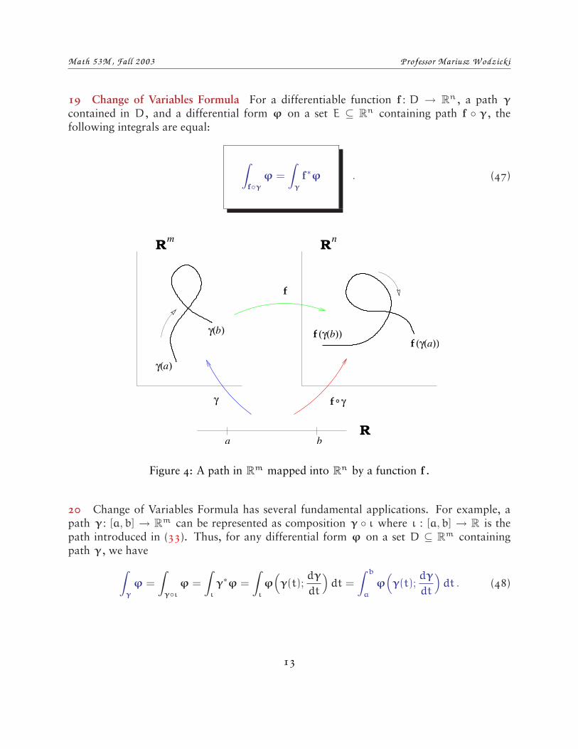
19 Change of Variables Formula For a differentiable function f : D → Rn , a path γ

contained in D, and a differential form ϕ on a set E ⊆ Rn containing path f ◦ γ, thefollowing integrals are equal:

∫f◦γ

ϕ =

∫γ

f∗ϕ . (47)

γ( )a

f (γ( ))

f

RnRm

a bR

fγ

γ( )b

° γ

f a(γ( ))b

Figure 4: A path in Rm mapped into Rn by a function f .

20 Change of Variables Formula has several fundamental applications. For example, apath γ : [a,b] → Rm can be represented as composition γ ◦ ι where ι : [a,b] → R is thepath introduced in (33). Thus, for any differential form ϕ on a set D ⊆ Rm containingpath γ, we have∫

γ

ϕ =

∫γ◦ι

ϕ =

∫ι

γ∗ϕ =

∫ι

ϕ(γ(t);

dγ

dt

)dt =

∫ b

a

ϕ(γ(t);

dγ

dt

)dt . (48)

13


since, as we noted in Section 14,∫

ι

fdt coincides with familiar Riemann13 integral∫ b

a

f(t)dt .

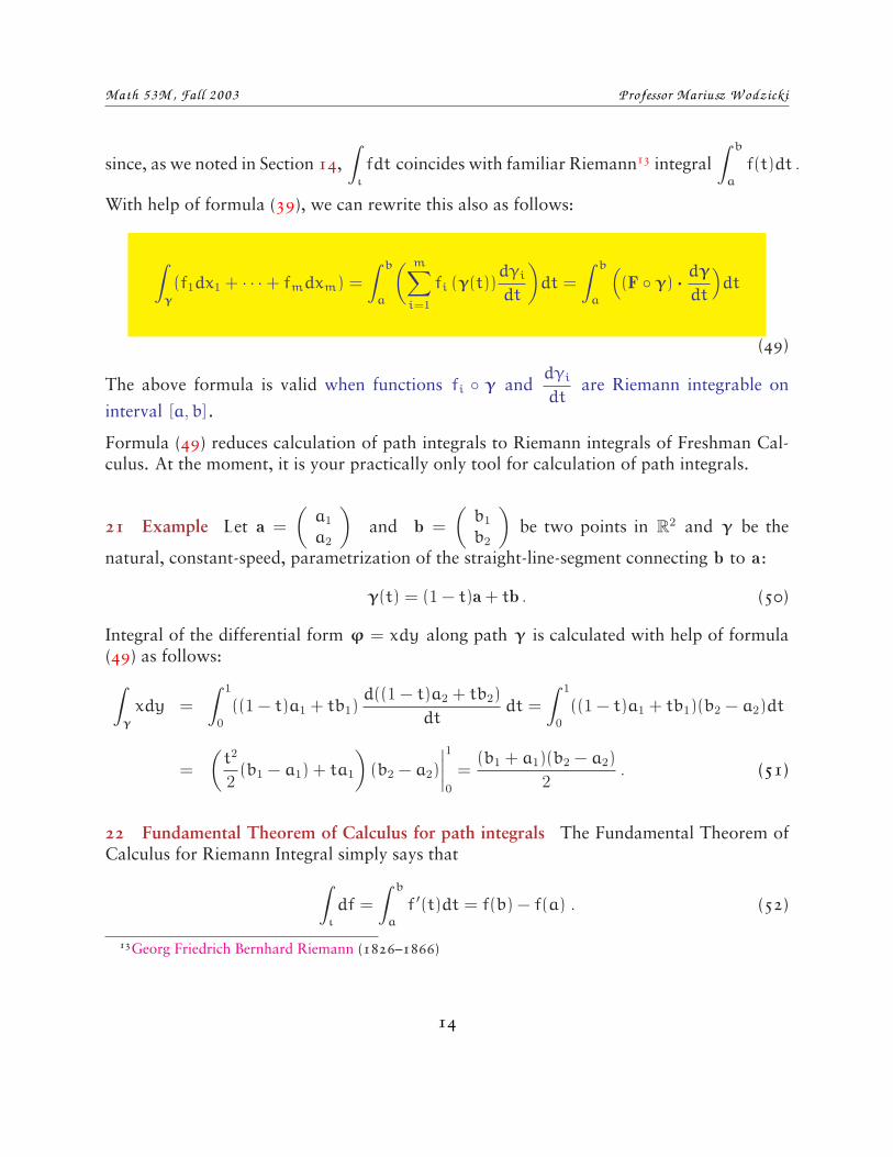
With help of formula (39), we can rewrite this also as follows:

∫γ

(f1dx1 + · · ·+ fmdxm) =

∫ b

a

( m∑i=1

fi (γ(t))dγi

dt

)dt =

∫ b

a

((F ◦ γ) · dγ

dt

)dt

(49)

The above formula is valid when functions fi ◦ γ anddγi

dtare Riemann integrable on

interval [a,b].

Formula (49) reduces calculation of path integrals to Riemann integrals of Freshman Cal-culus. At the moment, it is your practically only tool for calculation of path integrals.

21 Example Let a =

(a1

a2

)and b =

(b1

b2

)be two points in R2 and γ be the

natural, constant-speed, parametrization of the straight-line-segment connecting b to a:

γ(t) = (1 − t)a + tb . (50)

Integral of the differential form ϕ = xdy along path γ is calculated with help of formula(49) as follows:∫

γ

xdy =

∫ 1

0((1 − t)a1 + tb1)

d((1 − t)a2 + tb2)

dtdt =

∫ 1

0((1 − t)a1 + tb1)(b2 − a2)dt

=

(t2

2(b1 − a1) + ta1

)(b2 − a2)

∣∣∣∣10

=(b1 + a1)(b2 − a2)

2. (51)

22 Fundamental Theorem of Calculus for path integrals The Fundamental Theorem ofCalculus for Riemann Integral simply says that∫

ι

df =

∫ b

a

f ′(t)dt = f(b) − f(a) . (52)

13Georg Friedrich Bernhard Riemann (1826–1866)

14

http://www-gap.dcs.st-and.ac.uk/~history/Mathematicians/Riemann.html


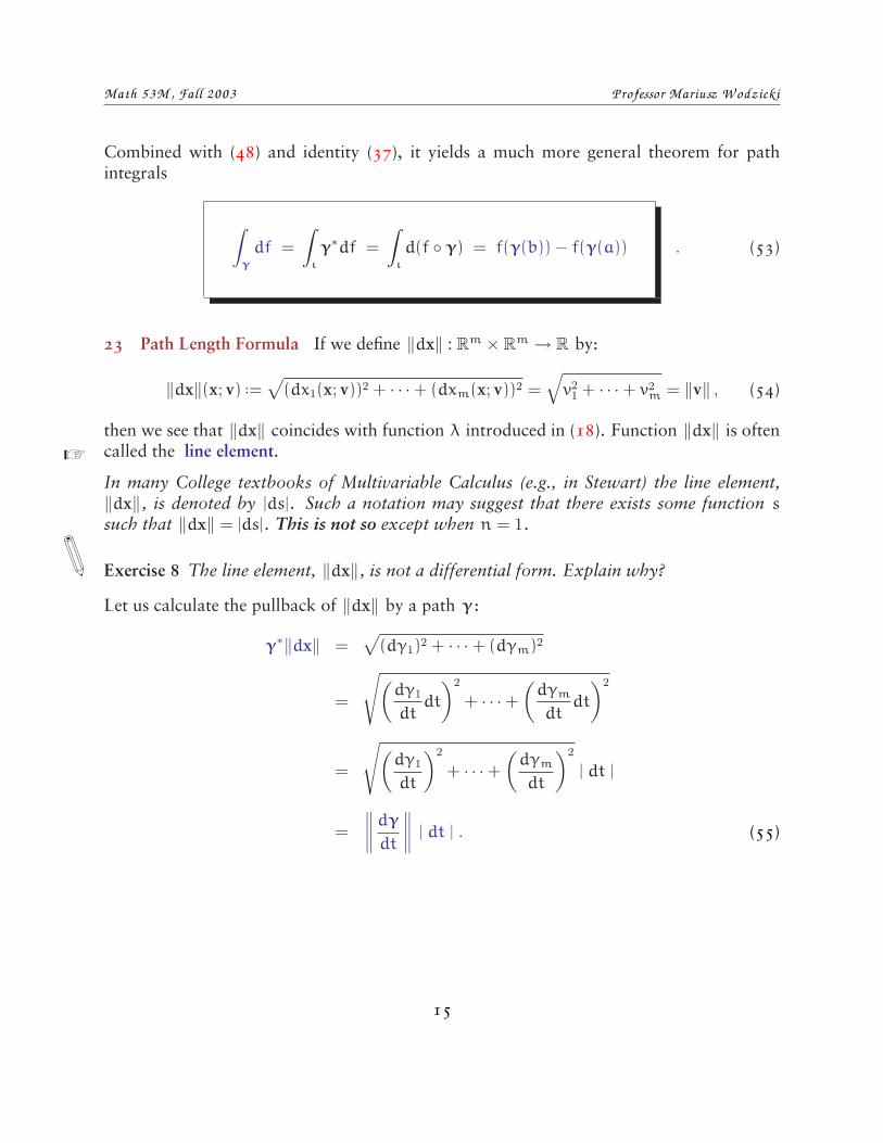
Combined with (48) and identity (37), it yields a much more general theorem for pathintegrals

∫γ

df =

∫ι

γ∗df =

∫ι

d(f ◦ γ) = f(γ(b)) − f(γ(a)) . (53)

23 Path Length Formula If we define ‖dx‖ : Rm × Rm → R by:

‖dx‖(x; v)˜√

(dx1(x; v))2 + · · ·+ (dxm(x; v))2 =

√v2

1 + · · ·+ v2m = ‖v‖ , (54)

then we see that ‖dx‖ coincides with function λ introduced in (18). Function ‖dx‖ is oftencalled the line element.RIn many College textbooks of Multivariable Calculus (e.g., in Stewart) the line element,‖dx‖, is denoted by |ds|. Such a notation may suggest that there exists some function ssuch that ‖dx‖ = |ds|. This is not so except when n = 1 .

W Exercise 8 The line element, ‖dx‖, is not a differential form. Explain why?

Let us calculate the pullback of ‖dx‖ by a path γ:

γ∗‖dx‖ =√

(dγ1)2 + · · ·+ (dγm)2

=

√(dγ1

dtdt

)2

+ · · ·+(dγm

dtdt

)2

=

√(dγ1

dt

)2

+ · · ·+(dγm

dt

)2

| dt |

=

wwwwdγdtwwww | dt | . (55)

15


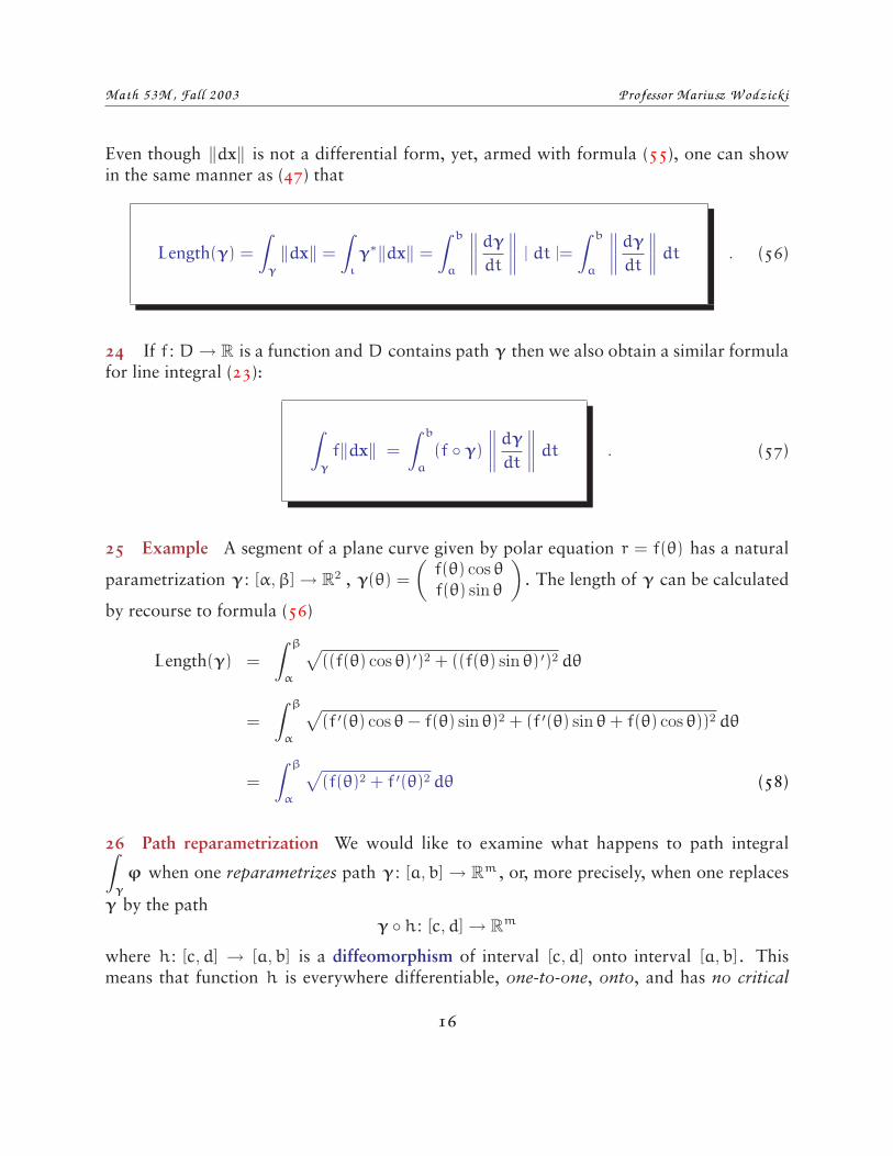
Even though ‖dx‖ is not a differential form, yet, armed with formula (55), one can showin the same manner as (47) that

Length(γ) =

∫γ

‖dx‖ =

∫ι

γ∗‖dx‖ =

∫ b

a

wwwwdγdtwwww | dt |=

∫ b

a

wwwwdγdtwwwwdt . (56)

24 If f : D→ R is a function and D contains path γ then we also obtain a similar formulafor line integral (23):

∫γ

f‖dx‖ =

∫ b

a

(f ◦ γ)

wwwwdγdtwwwwdt . (57)

25 Example A segment of a plane curve given by polar equation r = f(θ) has a natural

parametrization γ : [α,β] → R2 , γ(θ) =

(f(θ) cos θf(θ) sin θ

). The length of γ can be calculated

by recourse to formula (56)

Length(γ) =

∫ β

α

√((f(θ) cos θ) ′)2 + ((f(θ) sin θ) ′)2 dθ

=

∫ β

α

√(f ′(θ) cos θ− f(θ) sin θ)2 + (f ′(θ) sin θ+ f(θ) cos θ))2 dθ

=

∫ β

α

√(f(θ)2 + f ′(θ)2 dθ (58)

26 Path reparametrization We would like to examine what happens to path integral∫γ

ϕ when one reparametrizes path γ : [a,b] → Rm , or, more precisely, when one replaces

γ by the pathγ ◦ h : [c,d] → Rm

where h : [c,d] → [a,b] is a diffeomorphism of interval [c,d] onto interval [a,b]. Thismeans that function h is everywhere differentiable, one-to-one, onto, and has no critical

16


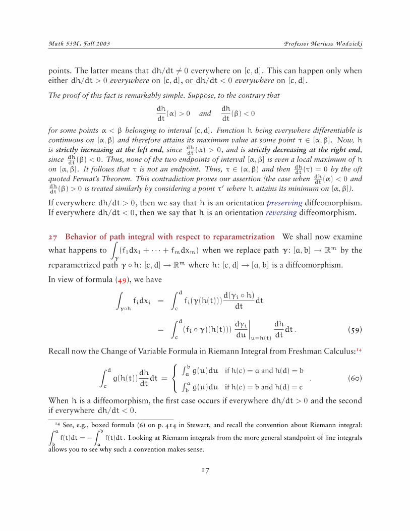
points. The latter means that dh/dt 6= 0 everywhere on [c,d]. This can happen only wheneither dh/dt > 0 everywhere on [c,d], or dh/dt < 0 everywhere on [c,d].

The proof of this fact is remarkably simple. Suppose, to the contrary that

dh

dt(α) > 0 and

dh

dt(β) < 0

for some points α < β belonging to interval [c,d] . Function h being everywhere differentiable iscontinuous on [α,β] and therefore attains its maximum value at some point τ ∈ [α,β] . Now, his strictly increasing at the left end, since dh

dt (α) > 0 , and is strictly decreasing at the right end,since dh

dt (β) < 0 . Thus, none of the two endpoints of interval [α,β] is even a local maximum of hon [α,β] . It follows that τ is not an endpoint. Thus, τ ∈ (α,β) and then dh

dt (τ) = 0 by the oftquoted Fermat’s Theorem. This contradiction proves our assertion (the case when dh

dt (α) < 0 anddhdt (β) > 0 is treated similarly by considering a point τ ′ where h attains its minimum on [α,β]).

If everywhere dh/dt > 0 , then we say that h is an orientation preserving diffeomorphism.If everywhere dh/dt < 0 , then we say that h is an orientation reversing diffeomorphism.

27 Behavior of path integral with respect to reparametrization We shall now examine

what happens to∫

γ

(f1dx1 + · · · + fmdxm) when we replace path γ : [a,b] → Rm by the

reparametrized path γ ◦ h : [c,d] → Rm where h : [c,d] → [a,b] is a diffeomorphism.

In view of formula (49), we have∫γ◦h

fidxi =

∫ d

c

fi(γ(h(t)))d(γi ◦ h)

dtdt

=

∫ d

c

(fi ◦ γ)(h(t)))dγi

du

∣∣∣∣u=h(t)

dh

dtdt . (59)

Recall now the Change of Variable Formula in Riemann Integral from Freshman Calculus:14

∫ d

c

g(h(t))dh

dtdt =

∫ b

ag(u)du if h(c) = a and h(d) = b∫ a

bg(u)du if h(c) = b and h(d) = c

. (60)

When h is a diffeomorphism, the first case occurs if everywhere dh/dt > 0 and the secondif everywhere dh/dt < 0 .

14 See, e.g., boxed formula (6) on p. 414 in Stewart, and recall the convention about Riemann integral:∫ a

b

f(t)dt = −

∫ b

a

f(t)dt . Looking at Riemann integrals from the more general standpoint of line integrals

allows you to see why such a convention makes sense.

17


By applying formula (60) to the function

g(u)˜ (fi ◦ γ)(u))dγi

du,

we infer that the last integral in (59) equals∫ b

a

(fi ◦ γ)(u))dγi

dudu =

∫γ

fidxi (61)

if h is orientation preserving, and equals

−

∫ b

a

(fi ◦ γ)(u))dγi

dudu = −

∫γ

fidxi (62)

if h is orientation reversing. Hence, for any differential form ϕ = f1dx1 + · · ·+ fmdxm , wehave the following identity

∫γ◦h

ϕ = ±∫

γ

ϕ (63)

with:

plus sign: when dh/dt > 0 everywhere on [c,d] , (63+ )

minus sign: when dh/dt < 0 everywhere on [c,d] . (63− )

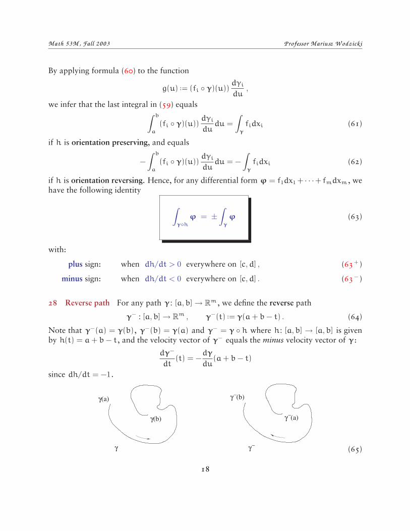
28 Reverse path For any path γ : [a,b] → Rm , we define the reverse path

γ− : [a,b] → Rm , γ−(t)˜ γ(a+ b− t) . (64)

Note that γ−(a) = γ(b), γ−(b) = γ(a) and γ− = γ ◦ h where h : [a,b] → [a,b] is givenby h(t) = a+ b− t, and the velocity vector of γ− equals the minus velocity vector of γ:

dγ−

dt(t) = −

dγ

du(a+ b− t)

since dh/dt = −1 .

γ(a)

γ(b)

γ

(a)γ−

−γ (b)

−γ (65)

18


Thus, the second case of identity (63) applies here and we obtain:∫γ−

ϕ = −

∫γ

ϕ . (66)

29 Equivalent parametrizations We shall say that two parametrizationsγ1 : [c,d] → Rm

and γ2 : [a,b] → Rm of a curve C are equivalent if

γ2 = γ1 ◦ h

for a suitable orientation preserving diffeomorphism h : [c,d] → [a,b], cf. condition (63+ ).From (63) we know that ∫

γ1

=

∫γ2

(67)

for equivalent parametrizations.

30 Regular arcs Recall from Section 24 in DCVF, that a path γ : [a,b] → Rm is regularif function γ has no critical points. This is equivalent to saying that the velocity-vectorfunction dγ

dtnowhere vanishes, see Section 26, Case m = 1 , in DCVF.

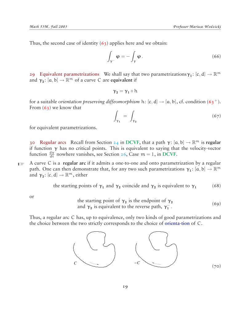
A curve C is a regular arc if it admits a one-to-one and onto parametrization by a regularRpath. One can then demonstrate that, for any two such parametrizations γ1 : [a,b] → Rm

and γ2 : [c,d] → Rm , either

the starting points of γ1 and γ2 coincide and γ2 is equivalent to γ1 (68)

orthe starting point of γ2 is the endpoint of γ2and γ2 is equivalent to the reverse path, γ−

1 . (69)

Thus, a regular arc C has, up to equivalence, only two kinds of good parametrizations andthe choice between the two strictly corresponds to the choice of orienta-tion of C.

C −C(70)

19


The latter corresponds to choosing which “end” of C is the starting point and which is theend point. If that choice is made, then one is dealing with an oriented regular arc C. Forsuch an arc we set ∫

C

ϕ ˜

∫γ

ϕ (71)

and ∫−C

ϕ ˜

∫γ−

ϕ (72)

where γ is any, one-to-one and onto, regular parametrization of oriented arc C. The mainpoint is that this definition does not depend on the choice of regular parametrization γ.

31 Oriented chains The proper setting for line integrals now reveals itself: we

integrate differential forms over “objects” Γ

which can be decomposed into a finite numberof regular oriented arcs C1 , . . . , Ck .

(73)

Such objects are called oriented chains. Thanks to additivity of path integral, cf. (14), theRquantity ∫

Γ

ϕ ˜

∫C1

ϕ + · · ·+∫

Ck

ϕ (74)

depends only on Γ and not on how Γ is decomposed into oriented arcs C1 , . . . , Ck .

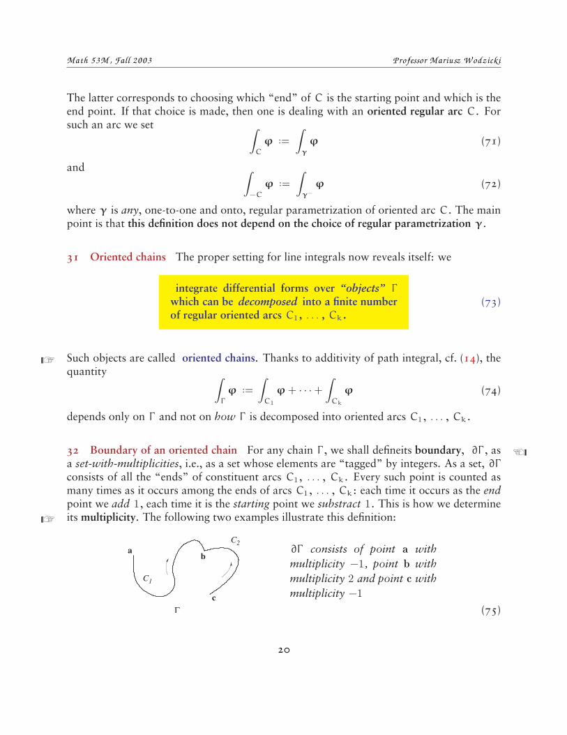
32 Boundary of an oriented chain For any chain Γ , we shall defineits boundary, ∂Γ , as La set-with-multiplicities, i.e., as a set whose elements are “tagged” by integers. As a set, ∂Γconsists of all the “ends” of constituent arcs C1 , . . . , Ck . Every such point is counted asmany times as it occurs among the ends of arcs C1 , . . . , Ck : each time it occurs as the endpoint we add 1 , each time it is the starting point we substract 1 . This is how we determineits multiplicity. The following two examples illustrate this definition:R

1C

2C

Γ

ab

c

∂Γ consists of point a withmultiplicity −1 , point b withmultiplicity 2 and point c withmultiplicity −1

(75)

20


1C

Γ

ab

c

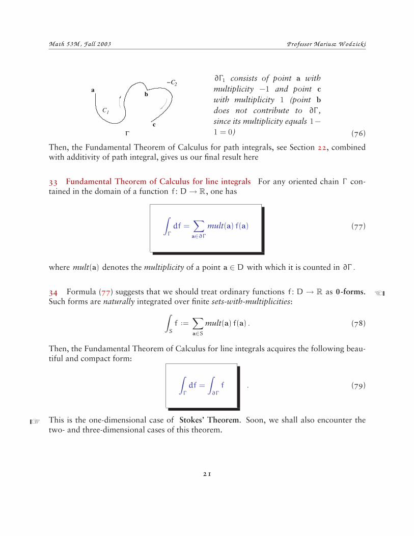
−C 2∂Γ1 consists of point a withmultiplicity −1 and point cwith multiplicity 1 (point bdoes not contribute to ∂Γ ,since its multiplicity equals 1−

1 = 0) (76)

Then, the Fundamental Theorem of Calculus for path integrals, see Section 22, combinedwith additivity of path integral, gives us our final result here

33 Fundamental Theorem of Calculus for line integrals For any oriented chain Γ con-tained in the domain of a function f : D→ R , one has

∫Γ

df =∑a∈∂Γ

mult(a) f(a) (77)

where mult(a) denotes the multiplicity of a point a ∈ D with which it is counted in ∂Γ .

34 Formula (77) suggests that we should treat ordinary functions f : D → R as 0-forms. LSuch forms are naturally integrated over finite sets-with-multiplicities:∫

S

f ˜∑a∈S

mult(a) f(a) . (78)

Then, the Fundamental Theorem of Calculus for line integrals acquires the following beau-tiful and compact form:

∫Γ

df =

∫∂Γ

f . (79)

This is the one-dimensional case of Stokes’ Theorem. Soon, we shall also encounter theRtwo- and three-dimensional cases of this theorem.

21


35 Cycles An oriented chain Γ is called a cycle if its boundary ∂Γ is empty. The Funda-mental Theorem of Calculus for cycles becomes:

∫Γ

df = 0 . (80)

We say that a differential form ϕ on D is exact if ϕ = df for a certain function f : D→ R .RIn this case, function f is called the primitive of ϕ.15 It follows from (80) that L

∫Γ

ϕ = 0 for any cycle Γ and any exact form ϕ . (81)

From Freshman Calculus we know that any continuous differential form ϕ on an intervalof real line is exact. Indeed, ϕ = gdt for a suitable continuous function g and, therefore,ϕ = df for the following antiderivative of g:

f(x)˜

∫ x

a

g(t)dt . (82)

The situation is very different, however, in higher dimensions.

36 Loop integrals and existence of the primitive A path γ : [a,b] → Rm that ends whereit starts:

γ(a) = γ(b) (83)

is called a loop. It follows from the Fundamental Theorem of Calculus for Path Integrals,(53), that ∫

γ

df = f(γ(b)) − f(γ(a)) = 0 (84)

for any loop γ, contained in the domain of function f, along which differential form df isintegrable.

15In traditional Physics courses, a function F : D → R3 , on a subset of R3 , is said to be a conservative Lvector field on D if differential form F · dx is exact. A function f : D → R such that df = F · dx (i.e., suchthat ∇f = F) is then called a potential for F .R

22


Now, let ϕ = f1dx1 + · · · + fmdxm be any differential form on a set D ⊆ Rm whose coef-ficient functions f1, . . . , fm are continuous. Such a form is integrable along any rectifiablepath in D. Suppose that∫

γ

ϕ = 0 for any rectifiable loop γ in D. (85)

Pick a point a ∈ D. Then for any two paths γ0 and γ1 contained in D, which connect apoint x ∈ D with a, the integrals of ϕ coincide:∫

γ0

ϕ =

∫γ1

ϕ . (86)

Indeed, without loss of generality we can assume that path γ0 is parametrized by interval[0, 1] while γ1 is parametrized by interval [1, 2] (we can choose equivalent parametrizationswithout changing the values of corresponding integrals, see Section 29). Then∫

γ0

ϕ −

∫γ1

ϕ =

∫γ0

ϕ +

∫γ−

1

ϕ =

∫γ0tγ−

1

ϕ = 0 . (87)

Here γ0 t γ−1 : [0, 2] → D is the loop starting and ending at a which traverses path γ0 for

0 6 t 6 1 and traverses path γ1 in reverse for 1 6 t 6 2 .

Thus, for differential forms satisfying condition (85), integral∫

γ

ϕ dependends only on the

path endpoints. This allows us to introduce the notation∫ x

aϕ˜

∫γ

ϕ (88)

where γ denotes any rectifiable path with starting point a and endpoint x. (Beware, how-ever, notation (88) makes sense only for forms satisfying condition (85).)

Suppose, for a moment, that every point x ∈ D can be connected by a (rectifiable) pathwith point a (we say, in this case, that set D is path-connected). Then, integral (88) defines La function of point x ∈ D whose differential equals ϕ (we omit verification of this fact).

23


We have established the following important theorem characterizing exact differential forms:

A differential form ϕ on a set D is exact if and only ifit satisfies condition (85). Its primitive is then given by

f(x) =

∫ x

aϕ

where a is a fixed point of D and x is any point of Dthat can be connected with a.

(89)

If set D ⊆ Rm is the disjoint union of path-connected components D1 , D2 , . . . , then wepick a ‘reference’ point ai ∈ Di in each path-connected component Di . This provides aprimitive for ϕ which is defined everywhere on D:

f(x) =

∫ x

ai

ϕ (for x ∈ Di ) . (90)

37 Example Consider the form

ϕ =xdy− ydx

x2 + y2 (91)

on the “punctured” plane, i.e., on the Euclidean plane with the origin removed:

D ˜{x ∈ R2 | x 6= 0

}. (92)

Let Cr be the counterclockwise oriented circle of radius r with center at the origin:

Cr ˜{x ∈ R2 | ‖x‖ = r

}. (93)

Circle Cr can be decomposed into any number of arcs, each naturally parametrized byangle θ:

γ(θ) ˜

(r cos θr sin θ

)(94)

By using formula (49), we thus obtain:

∫Cr

xdy− ydx

x2 + y2 =

∫ 2π

0

r cos θ(r cos θ) − r sin θ(−r sin θ)r2

dθ =

∫ 2π

0dθ = 2π (95)

Note that the result does not depend on radius r: it has the same value 2π for circlesarbitrary small or arbitrary large. In particular, form (91) is not exact.

24


38 Appendix: Proof of Formula (49) It is enough to show that, for any function f : D→R and integer 1 6 i 6 n, one has∫

γ

fdxi =

∫ b

a

f (γ(t))dγi

dtdt . (96)

Integral∫

γ

fdxi is the limit, when that limit exists, of finite sums

k∑j=1

(fdxi)(γ(t∗j ); γ(tj) − γ(tj−1)) =

k∑j=1

f(γ(t∗j )) (γi(tj) − γi(tj−1)) (97)

that we associate with tagged partitions P of interval [a,b], see (3). This means that

numbers (97) approach∫

γ

fdxi when the mesh of P , see (4), tends to zero.

Let us make a crucial assumption:

we assume that functions γi : [a,b] → R are differentiable . (98)

Then, by Mean-Value Theorem of Freshman Calculus,16

γi(tj) − γi(tj−1) =dγi

dt(t∗j ) (tj − tj−1) (99)

for some point t∗j ∈ [tj−1, tj]. Let us use these points t∗j to tag a given partition

a = t0 < t1 < · · · < tk = b . (100)

Thenk∑

j=1

f(γ(t∗j )) (γi(tj) − γi(tj−1)) =

k∑j=1

f(γ(t∗j ))dγi

dt(t∗j ) (tj − tj−1) . (101)

The sums on the right-hand-side of (101) converge to the Riemann integral∫ b

a

f (γ(t))dγi

dtdt (102)

if they converge at all. But they do, because sums (97) have a limit, namely∫

γ

fdxi . Thus,

we succeeded establishing two things. First, Riemann integral∫ b

a

f (γ(t))dγi

dtdt exists if

16Cf. e.g., Stewart, Section 4.2.

25


path integral∫

γ

fdxi exists and if, of course, function γi is differentiable on interval [a,b].

Second, these two integrals are equal.

Remarkably, the general Change of Variables Formula, (47), follows easily from (49) withhelp of pullback formula (42). Indeed, on one hand,∫

γ

g∗(fdxi) =

∫γ

(f ◦ g)dgj =

∫γ

(f ◦ g)

m∑j=1

∂gi

∂xj

dxj

=

∫ b

a

f(g(γ(t)))

m∑j=1

∂gi

∂xj

(γ(t))dγj

dt(t)dt by (49)

=

∫ b

a

f(g(γ(t)))(∇gi(γ(t)) ¨

dγ

dt(t)

)dt (103)

which, in view of the Chain Rule, see (23) in DCVF, equals∫ b

a

f(g(γ(t)))d((g ◦ γ)i)

dt(t)dt =

∫ b

a

f((g ◦ γ)(t))d((g ◦ γ)i)

dt(t)dt . (104)

This last integral equals∫

g◦γfdxi by formula (96), as desired.

Note that we established the Change of Variables Formula under assumption that path γ

is differentiable.

26

Documents

Line Integrals - University of California, Berkeleywodzicki/H185.S11/podrecznik/li.pdf · Line Integrals October 23, 2003 ... 1Abbreviation DCVF stands for Differential Calculus of