Embed Size (px)
Citation preview
Chapter 18
Receptor Modeling of Epiphytic Lichens to Elucidate the Sources and Spatial
Distribution of Inorganic Air Pollution in the Athabasca Oil Sands Region
M.S. Landis*, J.P. Pancras, J.R. Graney, R.K. Stevens, K.E. Percy and S. Krupa
*Corresponding author: e-mail address: [email protected]
Abstract
The contribution of inorganic air pollutant emissions to atmospheric deposition in the
Athabasca Oil Sands Region (AOSR) of Alberta, Canada was investigated in the
surrounding boreal forests, using a common epiphytic lichen bio-indicator species
(Hypogymnia physodes) and applying multiple receptor models. Source materials from
anthropogenic and natural emitters of air pollution in the AOSR were obtained and
chemically characterized to aid in the assessment. The lichens selected for analysis were
collected in 2008 using a stratified, nested grid approach radiating away from the central
area of oil sands production, at 121 sampling sites extending as far as 150 km. Source
and lichen samples were extracted and analyzed for 43 elements using dynamic reaction
cell inductively coupled plasma mass spectroscopy (DRC-ICPMS). Source
apportionment of the lichen tissue analytical results was conducted using Principal
Component Analysis (PCA), Chemical Mass Balance (CMB), Positive Matrix
Factorization (PMF), and Unmix Models.
Initial Varimax rotated PCA screening analysis indicated that there were five principal
components that could explain 89% of the variance contained in the lichen data set, with
the majority of the variance lumped into a fugitive dust factor. This fugitive dust source
could be separated into tailings sand, haul road, and overburden components using CMB
on lichen samples collected near the mining and oil processing facilities. However, the
CMB model performance was limited by the similarity of sources and the lack of total
nitrogen measurements in the emission source profiles. The PMF and Unmix models
were found to perform best with this unique AOSR lichen data set, providing very similar
results at near source as well as remote lichen collection sites. The PMF results showed
that sources significantly contributing to concentrations of elements in the lichen tissue
include: combustion processes (~23%); tailing sand (~19%); haul roads and limestone
(~15%); oil sand and processed materials (~15%); and a general anthropogenic urban
source (~15%).
The spatial patterns of CMB, PMF, and Unmix receptor models estimated that source
impacts on the Hypogymnia physodes tissue elemental concentrations from the oil sand
processing and fugitive dust sources had a significant association with the distance from
the primary oil sands surface mining operations and related production facilities. The
spatial extent of the fugitive dust impact was limited to an approximately 20 km radius
around the major mining and oil production facilities indicative of ground level coarse
particulate fugitive emissions from these sources. The impact of the general urban source
was found to be enhanced in the southern portion of the sampling domain in the vicinity
of the Fort McMurray urban area. The receptor model results showed lower Mn
concentrations in lichen tissues near oil sands production operations suggesting a
biogeochemical response. Overall the largest impact on elemental concentrations of
Hypogymnia physodes tissue in the AOSR was related to fugitive dust, suggesting that
implementation of a fugitive dust abatement strategy could minimize the near-field
impact of future mining related production activities.
1. Introduction
The Athabasca Oil Sands Region (AOSR) in northern Alberta, Canada contains
recoverable petroleum reserves estimated to be in excess of 170 billion barrels consisting
mostly of bitumen (Attanasi and Meyer, 2010). These proven reserves rank the AOSR
third in the world behind only Saudi Arabia and Venezuela. Oil production in the AOSR
has been steadily increasing over the last decade from 0.6 million barrels per day in 2000,
to 1.6 million barrels per day in 2011. Production is expected to be in excess of 3.5
million barrels per day by 2020. Synthetic crude oil production from bitumen in the
AOSR is accomplished using a combination of surface mining and in situ production. Of
the proven reserves, it is estimated that 20% of the bitumen will ultimately be recovered
through surface mining and 80% from in-situ production techniques (Government of
Alberta, 2008). The type and magnitude of inorganic air pollutants emitted from these
two extraction techniques are unique. Quantifying their relative contribution to observed
ambient concentrations and atmospheric deposition are critical to be able to mitigate and
manage local environmental impacts as production levels are increased.
Surface mining in the AOSR results in large scale land disturbance and is similar to coal,
copper, and other traditional mining operations. Currently, the soil and glacial till
overlaying the deposits (over burden) is removed and the exposed oil sands are excavated
and transported for processing using large scale shovel and truck hauling operations.
Atmospheric pollution from shovel and truck fleet operations mainly consists of fugitive
particulate matter (PM) emissions (wind-blown dust) and diesel engine combustion
exhaust. Bitumen is separated from sand and clay components and recovered using a
warm water separation technique. The water, sand, and clay waste stream is pumped to
large tailings ponds where the water is removed and recycled; and the sand and clay are
consolidated and used for mine reclamation activities. After the oil sands are removed
the miners reach the underlying limestone bedrock. The limestone is quarried, crushed,
and used for development of haul roads and other construction activities. Over burden
stored for future mine reclamation, haul roads, and tailings ponds are all potential sources
of fugitive wind-blown dust.
In-situ production refers to the extraction of bitumen from oil sand deposits that are
present at depths that make it uneconomical to access using traditional surface mining
(currently about 75 meters), and using techniques to separate the bitumen in place. Steam
assisted gravity drainage (SAGD) is currently the main in-situ stimulation technique
employed. SAGD involves the drilling of two parallel wells, one over the other. Steam
is injected into the upper well to thermally separate the bitumen from the host material.
The reduced viscosity of the heated bitumen causes it to drain down into the second
underlying well where it is pumped to the surface and recovered. The natural gas- and
syngas-fired boilers used to generate the steam are sources of atmospheric pollutant
emissions (e.g., NO, NOx).
The bitumen recovered from the AOSR is considered a “sour” extra heavy crude oil
(Attanasi and Meyer, 2010). The bitumen has a high specific gravity (>10ºAPI), is
extremely viscous at ambient temperatures, and contains elevated concentrations of sulfur
(>0.5%), and some metals (e.g., nickel, vanadium). The bitumen is upgraded to synthetic
crude oil by thermal/catalytic cracking to break down large long chain molecules and
removing excess sulfur (hydro-desulfurization) to facilitate the production of valuable
light (e.g., gasoline) and medium (e.g., diesel) distillate fuels. Some facilities upgrade the
bitumen to synthetic crude on site in the AOSR while others dilute the bitumen with
naptha and transport it to refineries via pipeline to other parts of Canada or the United
States. Upgrading, refining, and power generation are significant sources of atmospheric
NO, NOx, PM, and SO2 emissions. In addition to the anthropogenic sources of
atmospheric emissions from the petroleum industry in the AOSR, there are significant
light duty mobile source emissions, commercial boilers, and residential heating sources
as well as natural pollutant emitters such as forest fires.
The AOSR is located in a remote boreal forest ecosystem. Other than Fort McMurray,
much of the region has no ready access by land transportation and is not serviced by
commercial electric power infrastructure. Active ambient monitoring is limited to Fort
McMurray and a relatively narrow north/south transportation corridor. Therefore, the
Wood Buffalo Environmental Association (WBEA) Terrestrial Environmental Effects
Monitoring program (TEEM) used the epiphytic lichen, Hypogymnia physodes,
predominantly growing on jack pine (Pinus banksiana) and black spruce (Picea
mariana), as a bio-indicator of the atmospheric deposition and accumulation of air
pollutants for on-going terrestrial impact assessment. Hypogymnia physodes was
selected as the bioindicator species of choice because it is an epiphytic lichen that
extracts all its nutrients from the air, has a high tolerance for SO2, is prevalent in all areas
of the AOSR, and is commonly used in air quality monitoring (Garty, 2001; Jeran et al.
2002). Our investigation focused on total sulfur (S), total nitrogen (N) (Berryman et al.,
2010), 43 metals, stable isotopes of lead (Pb) (Graney et al., this volume), mercury (Hg)
(Blum et al., this volume), and poly-aromatic hydrocarbons (Studabaker et al., this
volume). Initially, spatial maps of S and N accumulation in the lichen were developed
for locations up to 150 km from the center of the oil sands production- emission source
area, with sampling at sites distributed as a nested grid. Based on the S and N
distributions, metals and the Pb and Hg isotopes were quantified at a subset of the lichen
sampling locations and the contributions of specific emission types were investigated
(Graney et al., this volume; Blum et al, this volume).
Deterministic or atmospheric dispersion models are routinely used by environmental
managers and government regulators as a tool to estimate the transport, transformation,
and deposition of atmospheric pollutants (Davies this volume). The ability of these
models (e.g., CALPUFF, CMAQ, ISC3, AERMOD) to reliably simulate the fate of
emitted pollutants on the spatial scales of interest in the AOSR are highly dependent on
the (i) quality of emission inventory data, (ii) completeness of the chemical kinetics
module, (iii) accuracy and resolution of the underlying gridded meteorological fields, (iv)
topography, and (v) proper parameterization of gas/particle interaction and wet and dry
deposition phenomena. In practice, it is extremely difficult to accurately model air
pollution in remote areas such as the AOSR where non-point mobile sources, fugitive
sources, batch processes, and forest fires are significant emission sources; and where few
local meteorological measurements are available for 4 dimensional data assimilation to
“nudge” the underlying meteorological drivers.
Receptor models provide another approach to understanding the impacts of air pollution
sources since the model results are based on measurement data at receptor or sampling
locations. Receptor models quantify the impact of air emission sources retrospectively
by using advanced mathematical methods on a matrix of elements or compounds in
atmospheric samples, or bio-indicators, as tracers for the presence of materials from
specific sources (Gordon 1985; Hopke 1985; Hopke 2009). The goal of receptor
modeling is to apportion the sources into specific identifiable categories (e.g.,
combustion, refining, motor vehicles, incineration, metals smelting, etc.) and quantify
their relative importance. Receptor models can also be used to constrain the uncertainty
in deterministic modeling estimates and help identify sources that may not be accurately
represented in emission inventories.
The main objectives of this study were to: (i) identify the major sources of air pollution
in the AOSR, (ii) collect and analyze samples to develop chemical source profiles (finger
prints), (iii) conduct a quantitative source apportionment analysis to determine the major
sources impacting the atmospheric deposition and accumulation of potentially phyto-
toxic levels of S and N in the tissue of Hypogymnia physodes, and (iv) provide supportive
data for Forest Health Monitoring (Krupa; Percy et al., Chapter 9, this volume).
2. Methods
2.1 Lichen Sampling and Analysis
A discussion on the selection of Hypogymnia physodes as a species for study can be
found in Graney et al. (this volume). A complete description of the collection, selection
strategy, and analysis methods for the Hypogymnia physodes samples is contained in
Edgerton et al. (this volume). Briefly, in 2008 WBEA-TEEM funded the collection of
lichen samples from 369 sampling locations using a stratified nested grid approach, with
higher density sampling at the center of the grid in close proximity to the main oil sands
production sites (Figure 1 in Edgerton et al., this volume). All samples were analyzed for
total S and total N at the University of Minnesota Research Analytical Laboratory
(UMRAL) (Berryman et al., 2010). A subset of samples from 121 of the sites was
selected for total microwave assisted acid extraction and analysis for 43 elements using
dynamic reaction cell quadrupole inductively coupled plasma-mass spectroscopy (DRC-
ICPMS) (Edgerton et al. this volume).
2.2 Source Sampling and Analysis
Bulk material samples representing the various steps in the oil sands production cycle and
other background materials were collected by WBEA for our analysis including: over
burden, raw oil sand, aged oil sand, limestone, materials used to construct haul roads,
bitumen, fluid coke, petroleum coke, vacuum tower bottoms, tailings sand, and ash from
forest fires. All bulk samples were extracted and analyzed by Atmospheric Research &
Analysis (ARA; Cary, NC) using the same total microwave assisted acid extraction and
DRC-ICPMS analysis methods used on the lichen samples (Edgerton et al. this volume).
In addition, diluted source sample emissions were collected as particulate material on
filters from the main stacks of an AOSR upgrading facility by Dessert Research Institute
(DRI) (Wang et al. this volume) and the exhaust of heavy duty hauling trucks by DRI
(Watson et al. this volume), as well as ambient PM2.5 on filters collected by WBEA at
Fort McKay during forest fire heavy smoke impacted days (PM2.5 > 420 g m-3) were
extracted and analyzed by ARA using DRC-ICPMS.
2.3 Theory and Concepts of Source Apportionment and Receptor Models
According to Hopke (2009) source apportionment is the estimation of the contributions to
the pollutant concentrations resulting from emissions from multiple natural and
anthropogenic sources. Forensic data (mathematical and/or statistical) analysis tools
called receptor models are applied to extract information on the sources of air pollutants
from the measured constituent concentrations at receptor location. Unlike deterministic
dispersion air quality models, receptor models generally do not use pollutant emissions,
meteorological data, and chemical transformation mechanisms to estimate the
contribution of sources to receptor concentrations. Instead, receptor models use
mathematically detectable characteristics (chemical and physical) of gases and particles
measured at a monitoring or receptor site to both identify and quantify source
contributions to receptor concentrations. These models are therefore a natural
complement to deterministic air quality models. The United States Environmental
Protection Agency (EPA) Office of Research and Development has developed several
integrated receptor modeling software tools such as Chemical Mass Balance (CMB),
Unmix, and Positive Matrix Factorization (PMF). Each of the EPA implemented
receptor model programs have a graphical user interface, data screening and analysis
tools, and data visualization capabilities. EPA has made all of these models available to
the public for use by students, researchers, industry, and government regulators
(http://www.epa.gov/scram001/receptorindex.htm, last accessed on June 13, 2012).
Typically, receptor models use repeated measurements of the chemical composition data
for airborne PM samples collected at a monitoring site (spatially fixed, temporally
resolved). In such cases, the outcome is the identification of the pollution source types
and estimates of the contribution of each source type to the observed concentrations
(Table 1). In lieu of a lack of sufficient data on the chemical composition of PM in
AOSR, we used data from the epiphytic lichen, Hypogymnia physodes, as an accumulator
or bio-indicator of various elements through atmospheric wet and dry deposition (Sloof,
1995; Kuik et al. 1993). It is believed that Hypogymnia physodes samples represent 3-5
years of accumulated atmospheric deposition in their tissue (Berryman et al., 2010;
Davies, this volume). We developed our AOSR epiphytic lichen concentration data
matrix based on samples collected at 121 locations in 2008 (spatially resolved,
temporally fixed).
2.3.1 Principal Component Analysis
Principal component analysis (PCA) is often used as a preliminary data reduction
technique to identify a small number of factors that explain most of the variance observed
in a much larger number of measured variables. According to Jolliffe (2002), PCA is
probably the oldest (first introduced in 1901) and best known techniques of multivariate
analysis. Like many multivariate methods, it was not widely used until the advent of
computers, but it is now available in virtually every statistical computer software
package. The central idea of PCA is to reduce the dimensionality of a data set in which
there are a large number of interrelated variables, while retaining as much as possible of
the variation present in the data set. This reduction is achieved by transforming the data
to a new set of variables, the principal components that are minimally correlated.
Principal components may be viewed as the eigenvectors of a positive semi-definite
symmetric matrix. The eigenvectors are “characteristic” vectors of a matrix. They are
unique in that they remain directionally invariant under linear transformation by its parent
matrix. Thus the definition and computation of principal components are straightforward
and has a wide variety of applications (e.g., Pratt et al. 1985; Voukantsis, 2011). The
general form for the equation (1) to compute scores on the first (main) component
extracted (created) in a principal component analysis:
C1 = b11 (X1) + b12 (X2) + ... b1p (Xp) (1)
Where,
C1 = the subject’s score on principal component 1 (the first component extracted);
b1p = the regression coefficient (or weight) for observed variable p, as used in creating
principal component 1, and Xp = the subject’s score on observed variable p.
In previous air pollution studies, the principal components have been found to represent
sources such as soil, motor vehicles, iron and steel production, metal smelting, coal
combustion, incineration and oil combustion (Hopke et al., 1976; Gaarenstroom et al.,
1977). In many cases, interpretations of the principal components have been difficult
because most of the variability of the data was loaded onto a single component (Thurston
and Spengler, 1985). This is not surprising, since PCA is designed to incorporate the
maximal amount of variance into the first factor (Hopke, 1985). Varimax orthogonal
rotation was performed in a manner described by Harmon (1976) to make physical
interpretation of the principal components easier (Thurston, 1981). Only rotated
principal components with eigenvalues >1 are typically retained for consideration
(Hopke, 1983).
Thurston and Spengler (1985) introduced an absolute principle component (APC) scores
calculation scheme by introducing an arbitrary zero-concentration sample wherein all
elemental concentrations are zero. Regressing mass concentration data on the APC
scores gave estimates of the coefficients which convert the APC score into pollutant
source mass contribution for each sample. An attractive feature of this modeling
framework is that no prior knowledge of the number or chemical composition of possible
sources is required. However, some of the major chemical characteristics of the emission
source must be present to correctly attribute the PC to a particular source type.
2.3.2 Chemical Mass Balance
EPA implemented CMB version 8.2 was used for this analysis (U.S. EPA, 2004). In
receptor modeling, a mass balance equation can be written to account for “m” chemical
species in the “n” samples as contributions from “p” independent sources (equation 2).
2
where, xij = the measured concentration of the jth species in the ith sample, fkj = the
concentration of the jth species in material emitted by source p, gik = the contribution of
the pth source to the ith sample, and eij = the portion of the measurement that cannot be
fitted by the model.
If the number and nature of the sources in the region are known (e.g., p and fpj's), then the
only unknown is the mass contribution of each source to each sample, gip (Winchester
and Nifong, 1971 and Miller et al., 1972). The problem is typically solved using an
effective-variance least-squares approach (Cooper et al., 1984) that is generally referred
to as the Chemical Mass Balance (CMB) model (Watson et al., 1990; US EPA, 2004). In
an ideal case, location specific source profiles are generated using the same extraction
and analytical techniques as the receptor samples. Typically this type of source
characterization is not feasible, and profiles from a source library are utilized such as
those available in the EPA SPECIATE version 4.3, profile repository
(www.epa.gov/ttn/CHIEF/software/speciate, last accessed on June 13, 2012). In this case
AOSR specific source profiles were generated (see Section 3.1).
Three statistical measurements are commonly used to evaluate - CMB model’s ability to
match the calculated species concentrations and the receptor data (U.S. EPA, 2004b) -: r2
values, chi square values, and the percent of total mass explained by the fit. An r2 value
is the fraction of the variance in the measured concentrations explained by the variance in
the calculated species concentrations. It is determined by linear regression of calculated
versus model-measured values for the fitting species. Ranges are from 0 to 1, with values
>0.8 indicating that the measured concentrations are well explained by the source
contribution estimates. The chi square value is the weighted sum of squares of the
differences between the measured and calculated element concentrations. Ideally, there
should be no difference, resulting in chi square of 0. A large chi square (>4.0) means that
one or more of the calculated species concentrations significantly differs from the
measured concentrations. The values for these statistics exceed their targets when: (i)
contributing sources have been omitted from the CMB calculation; (ii) one or more
source profiles have been selected which do not represent the contributing source types;
(iii) uncertainty estimates of receptor or source profile data are underestimated; and/or
(iv) errors or inconsistencies between analytical measurements used for source and
receptor data. Percent mass explained is the ratio of the difference between the sum of
the model-calculated source contribution estimates and the measured mass
concentrations. Ratios should equal to 100%, but values between 80% and 120% are
acceptable. In our CMB application the total variable (PM mass in lichen) is not
measurable. Also, receptor concentrations are normalized to lichen mass. As a result, the
CMB calculation estimates potential source contributions (‘g’ matrix in equation 2) in the
form of the total lichen mass concentration attributable to sources.
CMB is most useful for primary emissions where the chemical characteristics of the
particles are sufficient to characterize their apportionment. Inclusions of profiles for
secondary particles are difficult since they represent the product of atmospheric
transformations of gaseous emissions into particles and are generally treated as specific
chemical species such as sulfate, nitrate, and ammonium or ammonium sulfate and
ammonium nitrate. Unlike the multivariate receptor models like PMF and Unmix, CMB
can be used to determine contributions with a single sample.
2.3.3 Positive Matrix Factorization
EPA implemented Positive Matrix Factorization (PMF) version 4.2 was used for this
analysis (U.S. EPA, 2011). PMF is a constrained eigenvector, implicit least-squares
analysis aimed at minimizing the sum of squared residuals for the model. Paatero and
Tapper (2003) showed that in a PCA analysis, there is scaling of the data by column or by
row and that scaling will lead to distortions in the analysis. They further showed that the
optimum method for scaling uncertainty in the data matrix would be to scale each data
point individually. In this way, the more precise data will have more influence on the
solution than points that have higher uncertainties. However, point-by-point scaling
results in a scaled data matrix that cannot be reproduced by a conventional factor analysis
based on the singular value decomposition.
PMF allows each data point to be individually weighed. This feature allows the modeler
to adjust the influence of each data point, depending on the confidence in the
measurement. For example, data below detection can be retained for use in the model,
with the associated uncertainty adjusted so these data points have less influence on the
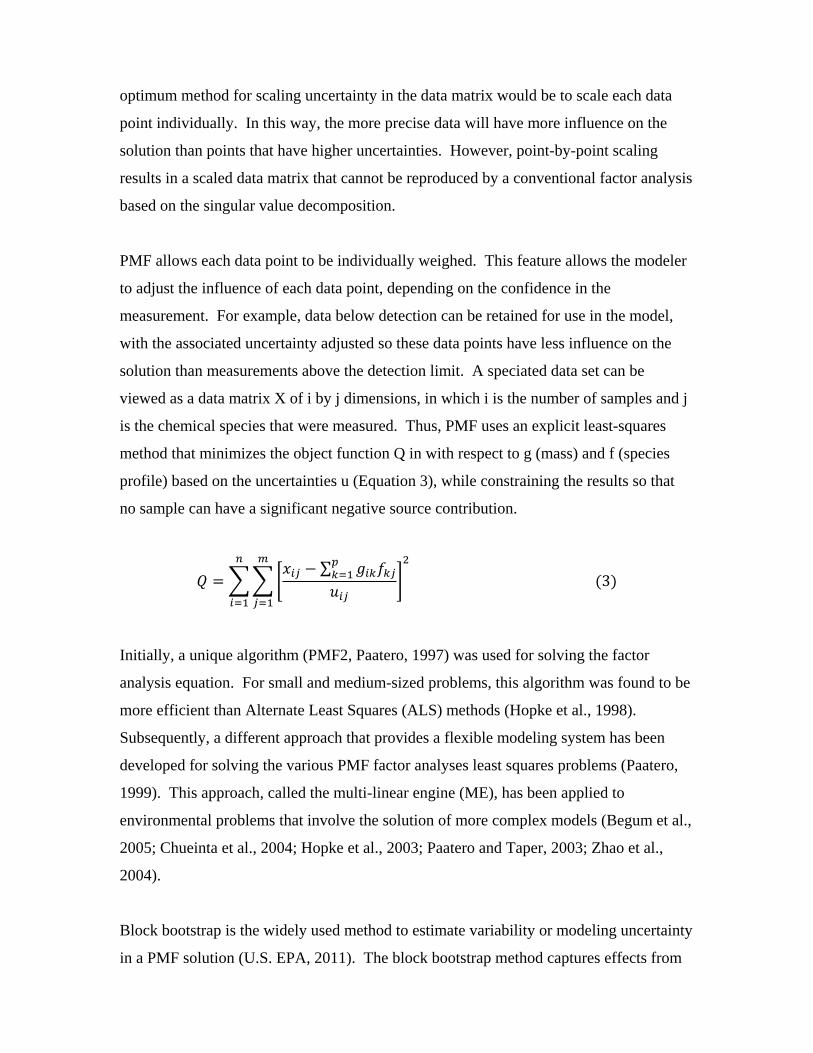
solution than measurements above the detection limit. A speciated data set can be
viewed as a data matrix X of i by j dimensions, in which i is the number of samples and j
is the chemical species that were measured. Thus, PMF uses an explicit least-squares
method that minimizes the object function Q in with respect to g (mass) and f (species
profile) based on the uncertainties u (Equation 3), while constraining the results so that
no sample can have a significant negative source contribution.
∑ 3
Initially, a unique algorithm (PMF2, Paatero, 1997) was used for solving the factor
analysis equation. For small and medium-sized problems, this algorithm was found to be
more efficient than Alternate Least Squares (ALS) methods (Hopke et al., 1998).
Subsequently, a different approach that provides a flexible modeling system has been
developed for solving the various PMF factor analyses least squares problems (Paatero,
1999). This approach, called the multi-linear engine (ME), has been applied to
environmental problems that involve the solution of more complex models (Begum et al.,
2005; Chueinta et al., 2004; Hopke et al., 2003; Paatero and Taper, 2003; Zhao et al.,
2004).
Block bootstrap is the widely used method to estimate variability or modeling uncertainty
in a PMF solution (U.S. EPA, 2011). The block bootstrap method captures effects from
random errors in the solution, and also partially accounts for errors from computational
rotational ambiguity. EPA - PMF performs bootstrapping by randomly selecting blocks
of samples, and creating a new input data of the selected sample, with the same
dimensions as the original dataset. PMF is then run on the newly created dataset, and
each factor from the bootstrap run is mapped to the base run factor by comparing the
contributions of each factor. The newly created bootstrap factor is assigned to the base
factor with which the bootstrap factor has the highest un-centered correlation above a
user-specified threshold. If no base factors have a correlation above the threshold for a
given bootstrap factor, that factor is considered ‘unmapped’. If more than one bootstrap
factor from the same run is correlated with the same base factor, they will all be mapped
to that base factor. This process is repeated for as many bootstrap runs as the user
specifies. A solution is considered valid when the occurrence of unmapped factors is less
than 10% of the total bootstrap runs. EPA - PMF reports variability in factor strengths as
various (5, 25, 50, 75, and 95) percentiles of factor strengths.
PMF2 was used to analyze data sets of major ion compositions of daily precipitation
samples collected at a number of sites in Finland (Juntto and Paatero, 1994) and bulk
precipitation (Anttila et al., 1995) to obtain information on the sources of those ions.
Polissar et al., (1996) applied PMF2 data from seven Alaska National Park sites to
resolve the major source contributions quantitatively.
Lee et al., (1999) applied PMF to urban aerosol compositions in Hong Kong. They were
able to identify up to 9 sources that provided a good apportionment of the airborne PM.
Similarly Huang et al., (1999) analyzed elemental composition of PM at Narragansett, RI
using both PMF and conventional PCA analysis. They were able to resolve more
components, with PMF using physically realistic compositions. Thus, the approach does
have some inherent advantages particularly through its ability to individually weight each
data point. PMF is somewhat more complex and harder to use, but it provides improved
resolution of sources and better quantification of those sources than PCA (Huang et al.,
1999).
Chueinta et al. (2000) introduced a directional source contribution analogous to a wind
“rose” to help provide information on the direction of the source relative to the receptor
site. Ramadan et al. (2000) applied PMF to a set of daily data from Phoenix, AR. In this
analysis, separate profiles were resolved for diesel and spark-ignition vehicles.
Analogously Lewis et al. (2003) analyzed the same data using Unmix and found similar
results for sources that contribute the largest amounts to the ambient mass concentrations.
Chemical composition of PM2.5 samples collected from1988 to 1995 at Underhill,
Vermont were analyzed by Polissar et al. (2001a). Sources representing wood burning,
coal and oil combustion, photochemical sulfate production, metal production plus
municipal waste incineration, and the emissions from motor vehicles were identified. In
addition emissions from smelting of nonferrous metal ores and arsenic, as well as soil
particles and particles with high concentrations of Na were identified by PMF.
2.3.4 Unmix
EPA implemented Unmix version 6.0 was used for this analysis (U.S. EPA, 2007).
Unmix is a constrained multivariate receptor model which seeks to solve a general
mixture problem where the data are assumed to be a linear combination of an unknown
number of sources of unknown composition which contribute an unknown amount to
each sample (Henry, 2003). Like PMF, Unmix also assumes that the compositions and
contributions of the sources are all non-negative. Unfortunately, it has been shown that
non-negativity conditions alone are not sufficient to give a unique solution and more
constraints are needed (Henry, 1987). To mitigate this constraint, Unmix assumes that
for each source there are at least a few samples that contain little or no contribution from
that source. This has been found to be a reasonable assumption since, in an ambient
monitoring example, the wind could be blowing away from the source, or for a lichen
bio-monitoring example the receptor location may be too far away from the source to
make a significant impact. Using only the concentration data for a given selection of
species, Unmix estimates the number of sources, source compositions, and source
contributions to each sample. It should be noted that, unlike PMF, Unmix does not allow
for down-weighting using data uncertainty values.
Unmix is also based on an eigenvalue analysis. The model uses a transformation method
based on the Self-Modeling Curve Resolution (SMCR) technique. The SMCR technique
identifies the feasible region of the real solution with explicit physical constraints, such as
source compositions must be non-negative. Explicit physical conditions form linear
inequality constraints in the space spanned by the eigenvectors, and these constraints
form the feasible region in eigenvectors’ space.
The Unmix model users manual (EPA, 2007) has a good description of how SMCR
identifies specific source impacts by using “edges”. Briefly, if the data consists of many
observations of M species, then the data can be plotted in an M-dimensional data space
where the coordinates of a data point are the observed concentrations of the species
during a sampling period. If there are N sources, the data space can be reduced to an (N-
1)-dimensional space. Edges are drawn using the assumption that for each source there
are some data points where the contribution of the source is not present or small
compared to the other sources. These are called edge points and Unmix works by finding
these points and fitting a hyper-plane through them; this hyper-plane is called an edge (if
N = 3, the hyper-plane is a line). By definition, each edge defines the points where a
single source is not contributing. If there are N sources, then the intersection of (N-1) of
these hyper-planes defines a point that has only one source contributing. Thus, this point
gives the source composition. In this way the composition of the N sources are found,
and from this the source contributions are calculated so as to give a best fit to the data.
As an example the model was applied to PM composition data from Phoenix (Lewis et
al., 2003). The analysis generated source profiles and overall average percentage source
contribution estimates for five source categories: gasoline engines (33 ± 4%), diesel
engines (16 ± 2%), secondary sulfate (19 ± 2%), crustal/soil (22 ± 2%), and biomass
burning (10 ± 2%). One of the unique aspects of this study was the ability to separate
motor vehicle contributions into separate diesel and gasoline sources. Diesel emissions
were identified by high elemental carbon relative to the organic carbon whereas gasoline
vehicles had a profile with more organic than elemental carbon. In addition, a substantial
difference was found in the contribution of diesel emissions between weekend and
weekday samples.
The Unmix’s use of hyper-plane edges was found to be particularly useful when
modeling high time resolution (30 min) PM2.5 measurements in Tampa, FL (Pancras et
al., 2011). Multiple sources such as residual oil combustion, lead smelting, coal
combustion, biomass burning, marine aerosol, general industrial, and a Cd-rich source
were clearly identified.
3. Results and Discussion
3.1 AOSR Source Characterization
The sources of inorganic atmospheric emissions in the AOSR are dominated by the
mining, processing, and upgrading of oil sand. While there are numerous sources of
emissions, most are different mixtures of similar components. The raw material that
drives the oil production activities in the AOSR is oil sand; made up primarily of sand,
clay, bitumen, and water. The mining and processing of the oil sand aims to separate the
bitumen (produced material) from the sand, clay, and water (tailings). The bitumen is
upgraded and refined creating targeted products such as synthetic crude, diesel fuel, and
gasoline; and byproducts such as petroleum coke and elemental sulfur (e.g., used in
agriculture). Petroleum coke is burned to produce electrical power and steam. Diesel is
used to fuel mining shovels, heavy haul trucks, and buses. Limestone and overburden are
used to construct haul roads. Tailing sand is processed and stored in large ponds for use
in mine pit reclamation. Superimposed over the oil sands mining and processing
emissions are regional contributions from forest fires, a common occurrence in the
AOSR. This reality makes source apportionment modeling a challenge in the AOSR.
The analytical results from the bulk material and stack test filters showed extensive
overlap or collinearity among the samples. We ultimately found it helpful to consolidate
similar source categories for developing the emission profiles for CMB, and interpreting
the PCA, PMF, and Unmix receptor modeling results. Table 2 summarizes the
composited source samples, their sample types, and sampling locations. Table 3 presents
the analytical emission profiles (mean ± standard deviation) for the consolidated sources
used in CMB model runs.
3.2 Modeling Information
Elemental concentrations measured in the Hypogymnia physodes samples that exhibited a
signal-to-noise ratio > 2 (2 above MDL; Edgerton et al., this volume) were chosen for
inclusion in PCA, CMB, PMF, and Unmix modeling. For PCA, CMB, and PMF runs a
total of 28 species were retained (Al, As, Ba, Ca, Ce, Cr, Cu, Fe, K, La, Li, Mg, Mn, Mo,
N, Na, Nd, Ni, P, Pb ,S, Se, Si, Sm , Sr, Ti, V, Zn). For Unmix runs, Ba and Ca were
dropped as better model fit statistics were observed in the absence of those two species.
Two samples exhibited several outlier concentration points, and were therefore excluded
from the data modeling. The following results are based on the remaining 119 samples.
Variation in elemental concentrations of a lichen specimen may arise due to its age,
chronic exposure, and the corresponding tissue gain or loss; and their governing genetic
and morphological variations. For those reasons, a total of ten-field duplicate samples
were also collected and analyzed. A mean relative percent deviation for every element
from the field duplicate results was then calculated and used as sampling precision in
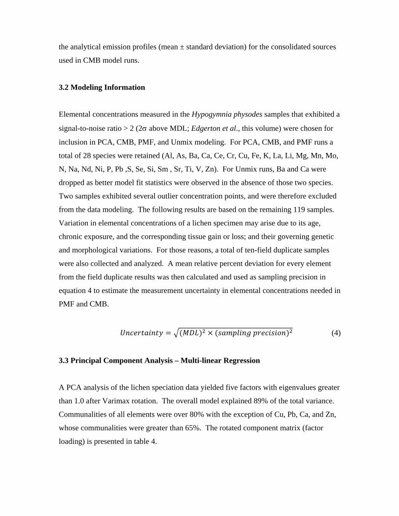
equation 4 to estimate the measurement uncertainty in elemental concentrations needed in
PMF and CMB.
(4)
3.3 Principal Component Analysis – Multi-linear Regression
A PCA analysis of the lichen speciation data yielded five factors with eigenvalues greater
than 1.0 after Varimax rotation. The overall model explained 89% of the total variance.
Communalities of all elements were over 80% with the exception of Cu, Pb, Ca, and Zn,
whose communalities were greater than 65%. The rotated component matrix (factor
loading) is presented in table 4.
The first factor component (FC #1) accounted for 58% of the total variance, and showed
high loadings of fossil fuel marker elements (V, Ni, Mo, As, Se), and crustal elements
(Li, Na, Al, Si, Ti, Fe, Mo, La, Ce, Nd, Sm). Given the AOSR source composition data
presented in Table 3, this factor very likely represents a composite of all coarse PM
sources such as oil sand, process material, and fugitive emissions. The FC #2 accounted
for 14% of the total variance with significant loadings for Mg, P, K, Ca, Sr, and Ba.
These elements are consistent with composition of the limestone bedrock material mined
in the AOSR region. FC #3 explained 7% of the total variance and has a high loading of
S and N. Oxides of sulfur and nitrogen can be either primary (stack) or secondary
products of high temperature combustion processes. Therefore, this factor likely
represents emissions from stack (stationary) and fleet vehicles (mobile). FC #4 presented
high loadings for Zn, Ba, and Cu, and accounted for 6% of the total variances.
Identification of this source is difficult since Zn, Ba, and Cu may be attributed to motor
vehicle brake/tire wear, combustion of synthetic lubricants, or general anthropogenic
activities. The last factor showed a strong negative loading for Mn. Graney et al., (this
volume) observed Mn depletion in Hypogymnia physodes near the active mining and
bitumen upgrading facilities, perhaps due to biological inhibition of uptake or losses from
tissue degradation. Nevertheless, it only accounted for 4% of the total variance, and
therefore FC #5 is neglected from further analysis.
Percent contribution of every element in a factor was determined by running a multi-
linear regression (MLR) model on each measured variable as dependant and all four
absolute factor scores as independent variables (Thurston, 1985). Table 5 summarizes
the apportionment of measured concentrations by the PCA-MLR method. Over 65% of
the measured concentrations of Al, Ce, La, Mo, Ni, Si, Ti, and V were found to
contribute to FC #1, which may be related to oil sand mining and processing activities.
Elevated Ca, P, and Sr contributions confirm FC #2 as limestone, while the 40-45% of
the measured N and S in FC #3 suggest that this factor is combustion related. Zn and Pb
are the dominant contributing elements to the factor identified as general anthropogenic.
A significant fraction of the measured Ba, Mg, S, Pb, K, and Zn concentrations were not
explained by the PCA-MLR model.
3.4 Chemical Mass Balance
The selection of appropriate source profiles is a challenge when utilizing CMB. In this
case, we used all the individual source sample profiles collected in the AOSR in the
initial CMB model runs. Many of the local sources were observed to be not estimable by
CMB due to excessive collinearity between the source profiles such as haul road dust
emissions, limestone bedrock, tailing sand, oil sand, and overburden samples. Crustal,
limestone, and oil component signatures (e.g., Ni, V) were present in all of these source
materials (because bitumen extraction from oil sand is not 100% quantitative). The
general CMB model (and other receptor models) assumes that (i) composition of source
emissions are constant over the ambient and source sampling period, (ii) chemical species
do not react with each other, (iii) chemical species add linearly, (iv) all major
contributing sources are identified and characterized, (v) number of sources are less than
the number of chemical constituent measured, (vi) source profiles are linearly
independent, and (vii) measurement error is available, and it is random, uncorrelated, and
normally distributed. However, studies show that deviations from one or more of the
above mentioned assumptions can still yield acceptable apportionment results.
Nonetheless, ‘nearly collinear’ sources affect CMB apportionment and often lead to
unacceptable solutions. Chemically similar sources without unique marker species to
distinguish between them are termed as collinear sources. If two or more sources exhibit
similar composition profiles, negative contributions are outputted by CMB. Such
situations can be mitigated by variable selection, (e.g., eliminating one or more analytical
species or entire sources that are nearly collinear). But, care must be taken to not to
eliminate a known source to improve the numerical performance of a receptor model.
Mined oil sand (raw material) is physically and chemically dissociated into bitumen
(target product), byproducts (petroleum coke), and residual materials (tailings). But the
individual sources can still retain chemical similarities. To illustrate this point, the linear
combination of tailing sand + processed material (y axis) is plotted against raw oil sand
(x axis) composition in Figure 1. Therefore, either oil sand or processed material and
tailing sand can be included in the model, but not all three together. Limestone source
material was also not included in the CMB run as this crushed bedrock construction
mineral was found to be collinear with the haul road dust source profile. Upon closer
examination, it was clear that the haul road dust profile was dominated by limestone
mineral. This finding was not surprising, because these temporary roads are constructed
primarily of mined limestone minerals, overburden, and low grade oil sand. Large
variability in emission signatures from the main upgrader stack and heavy-duty hauler
fleet source profiles were other major areas of concern as species with large uncertainties
are likely to be non-influential in the CMB apportionment (U.S. EPA, 2004b).
In order to overcome these obstacles, we combined similar source materials into
composite source profiles (Table 2) and re-ran the CMB model with these carefully
chosen seven local source profiles such as haul road dust, processed materials, tailing
sand, fleet vehicles, main upgrader stack, forest fire/wood smoke, and overburden. The
fit statistics (r2 >0.8 and chi square > 2) were excellent for samples collected near the
mining location, and worse for the distal samples. For receptors located within a 20 km
radius (n= 28), 72 ± 23% of the lichen mass was explained by these six sources. Median
PM contributions of haul road dust, processed materials, tailing sand, overburden, forest
fires, fleet vehicles, and main upgrader stack to the near field lichens were estimated to
be 242 ± 78, 190 ± 116, 178 ± 100, 87 ± 57, 45 ± 30, 6 ± 2, and 1 ± 0 mg g-1 of lichen
mass, respectively.
Figure 2 presents individual sample contribution as a function of distance (km) from the
center of the surface mining oil production activities. The strong influence of fugitive
dust from the oil sand mining and processing operations on the near field (<20 km) lichen
samples is clear. The relative magnitude of the fugitive dust sources was found to be
haul road>tailing sand>overburden. Distal samples (>20 km) were under-estimated
possibly because of under-representation of contributing sources in the CMB model
itself. Edgerton et al. (this volume) documented that the lichen tissue concentrations
collected in distal site locations were found to be lower in element concentrations than
other areas in North America. It has been observed that under-representing the number
of sources had little effect on the calculated source contribution estimates (SCEs) if the
dominant species of the missing sources were excluded from the solution (U.S. EPA,
2004b). Since the objective of this study is to evaluate air pollution from the AOSR
region, no further attempts were made to explain all of the measured concentrations in
distal receptor samples.
3.5 Positive Matrix Factorization and Unmix Modeling
3.5.1 Description of Factors
A six factor solution was found to be optimal by both the PMF and Unmix, models.
Figure 3 presents and compares the source profiles generated by the models. In general,
all factors showed good agreement between the two modeling approaches used, except
the factor attributed to combustion sources. The block bootstrap method was used to
evaluate modeling uncertainty in both PMF and Unmix solutions. There were not any
rejected (uncorrelated) factors from either model runs. Factor contributions were paired,
and linear regression analysis was performed between the pairs of Unmix and PMF factor
contribution estimates. As shown in Table 6, all of the six factors, interpreted as sources
in the following section, showed good agreement between the two modeling results (r2 >
0.5, slope > 0.6). The following source identifications are for PMF and Unmix
indentified factors:
Oil Sand & Processed Material: High loadings of V (59%), Ni (46%), Mo (51%), La
(34%), Ce (34%), and Sm (35%), with La/Ce and V/Ni ratios close to source material
values identifies this factor as the oil component in the oil sand + processed material
signature. Modeled V/Ni, and La/Ce ratios are 2.40 and 0.48, respectively. The
composite oil sand source profile contains V/Ni of 1.95 and La/Ce of 0.42. This factor
does not include a significant Ca loading, which is also a characteristic of oil sand source
profile. A source contribution estimate (SCE) map (Figure 4) depicts an area of high
source impact at the very center of the oil sand mining and processing activities. This
type of clear near-field enhancement is consistent with ground level emission of coarse
particle fugitive dust. Coarse PM is produced mainly by mechanical forces such as
crushing and abrasion, and therefore, consist primarily of finely well divided minerals
such as oxides of aluminum, silicon, iron, calcium, and potassium. Coarse particles of
soil or dust mostly result from entrainment by wind or from other mechanical action.
Since the size range of these particles are quite large, their corresponding deposition
velocities by sedimentation are relatively high. Therefore, particles retention time in the
atmosphere and transport scales are generally short, resulting in enhancement of near
field deposition gradients (Davidson and Wu, 1989; Landis and Keeler, 2002).
Fugitive Tailings Sand: This factor comprises elements Al, Si, Ti, Ca, Ba, La, and Sm
with large relative occurrence. The composite tailing sand source sample shows a close
resemblance with this factor. Since tailing sand is processed and has had the bitumen
removed, it is physically (smaller aggregate particle size) and chemically (lower
concentration of the oil tracer species such as Ni and V) different from the mined raw oil
sand particles. The SCE map (Figure 5) clearly supports that this factor is local to the
central oil sand mining and production areas, but with a slightly more easterly extent and
more widely distributed in space as compared to the oil sand factor. We therefore assign
this factor to represent local fugitive sand resulting from the exposed tailings ponds and
various ground based hauling activity.
Haul Road & Limestone Mixture: Elevated levels of Ca, Mg, Sr, and Ba characterize this
factor. The ratio of Ca/Sr and Ca/Mg are very close to the limestone source material
collected in the active mining areas. The limestone bedrock mined in this region
underlying the oil sands is used to construct temporary roads for truck hauling operations.
Spatial contribution estimates presented in Figure 6 matches our expectation with high
loading estimates near the active mining areas in 2008 and hauling road activity.
Combustion Source Emissions: S, N, P, K, and Cu contributed 47%, 39%, 52%, 42%,
and 26% of their respective modeled concentrations to this factor. Oxides of nitrogen
and sulfur are primarily combustion related emissions such as SAGD boilers and
upgrader main stacks (N, S) and fleet vehicle (P, Ca, Cu) emissions. The spatial
distribution of contributions (Figure 7) for this factor shows the area of highest impact
was farther away from the oil production facilities, which is consistent with an elevated
stack emitting a plume with thermal buoyancy. The impact of ecosite classification of
the lichen collection sites (Graney et al., this volume) showed significant differences for
this factor. Mean source contribution estimate from dry (1.5) sites were significantly
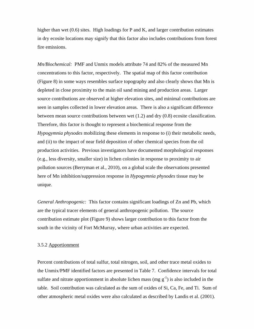
higher than wet (0.6) sites. High loadings for P and K, and larger contribution estimates
in dry ecosite locations may signify that this factor also includes contributions from forest
fire emissions.
Mn/Biochemical: PMF and Unmix models attribute 74 and 82% of the measured Mn
concentrations to this factor, respectively. The spatial map of this factor contribution
(Figure 8) in some ways resembles surface topography and also clearly shows that Mn is
depleted in close proximity to the main oil sand mining and production areas. Larger
source contributions are observed at higher elevation sites, and minimal contributions are
seen in samples collected in lower elevation areas. There is also a significant difference
between mean source contributions between wet (1.2) and dry (0.8) ecosite classification.
Therefore, this factor is thought to represent a biochemical response from the
Hypogymnia physodes mobilizing these elements in response to (i) their metabolic needs,
and (ii) to the impact of near field deposition of other chemical species from the oil
production activities. Previous investigators have documented morphological responses
(e.g., less diversity, smaller size) in lichen colonies in response to proximity to air
pollution sources (Berryman et al., 2010), on a global scale the observations presented
here of Mn inhibition/suppression response in Hypogymnia physodes tissue may be
unique.
General Anthropogenic: This factor contains significant loadings of Zn and Pb, which
are the typical tracer elements of general anthropogenic pollution. The source
contribution estimate plot (Figure 9) shows larger contribution to this factor from the
south in the vicinity of Fort McMurray, where urban activities are expected.
3.5.2 Apportionment
Percent contributions of total sulfur, total nitrogen, soil, and other trace metal oxides to
the Unmix/PMF identified factors are presented in Table 7. Confidence intervals for total
sulfate and nitrate apportionment in absolute lichen mass (mg g-1) is also included in the
table. Soil contribution was calculated as the sum of oxides of Si, Ca, Fe, and Ti. Sum of
other atmospheric metal oxides were also calculated as described by Landis et al. (2001).
Both models explained >97% of the measured total sulfur and total nitrogen
concentrations. Metal oxides contributions estimated by the two models differ. This was
most likely due to Ca not being included in the Unmix model (see Section 3.2). While
Unmix over-predicted other metal oxides, PMF did not explain 8% and 6% of the soil,
and other metal oxides contributions, respectively.
Nearly 40% of the measured sulfate and nitrate concentrations were explained by
combustion sources that include fleet vehicles, stack, and forest fire emissions. General
anthropogenic background emerges as the next significant source for sulfate and nitrate.
As expected, soil related contributions are significant from tailing sand fugitive dust and
haul road fugitive dust factors. Of all the sources identified, oil sand & processed
materials, tailing sand fugitive dust, haul road fugitive dust, and combustion emissions
are originating from the AOSR oil sand mining and production operations. Together,
these sources explain 72% of the measured element concentrations (as oxides) found in
Hypogymnia physodes tissue samples (Figure 10).
4. Conclusions
Overall the concentration of elements observed in Hypogymnia physodes tissue samples
in the boreal forests in the AOSR were consistent with those reported in other areas of
Canada, the United States, and in other areas in the northern hemisphere (Edgerton et al.,
this volume). However, near field samples collected within 20 km of the main surface
mining and oil sand production/upgrading operations had significantly higher
concentrations of both crustal (La, Ce, Nd, Ti, Fe, Ca, Sr) and anthropogenic elements
(Ni, V, Sn, Mo, Cr, Cu, Sb). The anthropogenic and natural sources of air pollution in
the AOSR including oil sands mining and processing activities and forest fires were
identified, sampled, and chemically characterized. The relative contributions of the
different inorganic air pollutant source types in the AOSR on the epiphytic lichen
Hypogymnia physodes tissue concentrations observed in the surrounding boreal forests
was investigated using PCA, CMB, PMF, and Unmix receptor models.
Initial PCA screening analysis indicated that there were five principal components that
could explain 89% of the variance contained in the lichen data set. Use of the CMB
model was hindered by source collinearity issues, but was able to successfully apportion
near field sampling locations (<20 km of mining and upgrading facilities). CMB
determined that six of the seven composited source profiles significantly contributed to
the near field lichen tissue concentrations. The PMF and Unmix multivariate receptor
models provided very consistent results, and indicated there were six significant source
factors. Five of the sources impacting the lichen tissue concentrations were primarily
anthropogenic including: (i) oil sand & processed material, (ii) tailing sand fugitive dust,
(iii) combustion processes, (iv) limestone & haul road fugitive dust, and a (v) general
urban source. The remaining significant source was a Mn dominated biogeochemistry
factor.
The spatial patterns of CMB, PMF, and Unmix receptor model estimated source impacts
on the Hypogymnia physodes tissue concentrations from the oil sand/produced material
and fugitive dust sources were significantly correlated to the distance from the primary
oil sands surface mining operations and related production facilities. The spatial extent
of the impact was approximately limited to a 20 km radius around the major mining and
oil production facilities which is clearly indicative of ground level coarse particulate
fugitive emissions from these sources. The relative impact of the general urban
background source was found to be enhanced in the lichens in proximity to the Fort
McMurray urban area. The receptor models also show a Mn related biogeochemical
response factor that is a combination of ecological factors (wet versus dry ecosite) as well
as a Mn response to near field oil sands production operations.
Overall the largest impact on elemental concentrations of Hypogymnia physodes tissue in
the AOSR was related to fugitive dust, suggesting that implementation of a fugitive dust
abatement strategy could minimize the near-field impact of future mining related
production activities. Over the next decade as oil production increases in the AOSR (i)
new surface mining operations will expand the footprint of land disturbance, (ii) in-situ
techniques will represent a larger percentage of overall bitumen extraction volume, (iii)
new production and upgrading technologies will improve extraction efficiencies while

reducing energy demand, (iv) new techniques for treating tailings will emerge, and (v)
mine remediation activities will accelerate. How these changes impact atmospheric
deposition in the surrounding boreal forests remains to be seen. It is recommended that
the combination of epiphytic lichen biomonitoring and the application of receptor models
continue to be used to inform residents in the AOSR on the impact of bitumen production
on their communities and natural forest resources.
5. Acknowledgements
We thank Shanti Berryman and Justin Straker (Stantec) for their efforts in lichen sample
collection and cleaning; Joel Blum (University of Michigan) for lichen sample grinding;
and Mike Fort and Eric Edgerton (Atmospheric Research & Analysis) for lichen sample
extraction and DRC-ICPMS analysis. This work was funded by WBEA. The EPA
through its Office of Research and Development collaborated in this research. It has
been subjected to EPA Agency review and approved for publication. The content and
opinions expressed by the authors do not necessarily reflect the views of the EPA,
WBEA, or the WBEA membership.
6. References
Alberta's Oil Sands: Opportunity, Balance. Government of Alberta, Edmonton, AB,
Canada. March 2008. ISBN 978-0-7785-7348-7.
Anttila, P., Paatero, P., Tapper, U. and Järvinen, O. (1995). Application of positive matrix
factorization to source apportionment: results of a study of bulk deposition chemistry in
Finland. Atmospheric Environment. 29:1705-1718.
Attanasi, E.D. and Meyer, R.F. (2010). Natural Bitumen and Extra-Heavy Oil - Survey of
energy resources (22 ed.). World Energy Council, London, UK. pp. 123–140. ISBN 0-
946121-26-5.
Begum, B., Hopke, P.K. and Zhao, W. (2005). Source identification of fine particles in
Washington DC by expanded factor analysis modeling. Environmental Science &
Technology. 55: 227-240.
Berryman, S., Straker, J., Krupa, S., Davies, M., Ver Hoef, J. and Brenner, G. (2010).
Mapping the characteristics of air pollutant deposition patterns in the Athabasca Oil
Sands Region using epiphytic lichens as bioindicators. Interim Report Submitted to the
Wood Buffalo Environmental Association, Fort McMurray, AB, Canada.
Cao, J., Li, H., Chow, J.C., Watson, J.G., Lee, S., Rong, B., Dong, J.G. and Ho, K.F.
(2011). Chemical composition of indoor and outdoor atmospheric particles at Emperor
Qin's Terra-cotta Museum, Xi’an, China. Aerosol and Air Quality Research.11:70-79.
Chan, Y.C.; Hawas, O.; Hawker, D.; Vowles, P.; Cohen, D.D.; Stelcer, E.; Simpson, R.;
Golding, G.; Christensen, E. (2011). Using multiple type composition data and wind data
in PMF analysis to apportion and locate sources of air pollutants. Atmospheric
Environment, 45: 439-449.
Cheng, Y., Lee, S.C., Cao, J.J., Ho, K.F., Chow, J.C. and Watson, J.G. (2009). Elemental
composition of airborne aerosols at a traffic site and a suburban site in Hong Kong.
International Journal of Environment and Pollution. 36:166-179.
Chow, J. and Watson, J. (2002). Review of PM2.5 and PM10 apportionment for fossil fuel
combustion and other sources by the chemical mass balance receptor model. Energy and
Fuels. 16: 222-260.
Chueinta, W., Hopke, P.K.and Paatero, P. (2000). Investigation of sources of atmospheric
aerosol urban and suburban residential areas in Thailand by positive matrix factorization.
Atmospheric Environment. 34: 3319-3329.
Chueinta, W., Hopke, P.K. and Paatero, P. (2004). A multi-linear model for spatial
pattern analysis of the measurement of haze and visual effects project. Environmental
Science & Technology. 38: 544-554.
Cooper, J.A., Watson, J.G. and Huntzicker, J.J. (1984). The effective variance weighting
for least squares calculations applied to the mass balance receptor model. Atmospheric
Environment. 18: 1347-1355.
Davidson, C.I. and Wu, Y.L. (2002). Dry Deposition of Particle and Vapors. In: Acidic
Precipitation. 3: Sources, Deposition and Canopy Interactions. Lindberg, S.E., Page,
A.L. and Norton, S.A. (eds.) Springer-Verlag, New York.
Faure, G. (1991). Principles and Applications of Inorganic Geochemistry, Macmillan Publishing Company, New York, New York.
Gaarenstroom, P.D., Perone, S. and Moyers, J. P. (1977). Application of pattern
recognition and factor analysis for characterization of atmospheric particulate
composition in southwest desert atmosphere. Environmental Science & Technology. 11:
7950-800.
Garty, J. (2001). Biomonitoring atmospheric heavy metals with lichens: Theory and
application. Critical Reviews in Plant Science. 20 (4): 309-371.
Gordon, G.E. (1985). Receptor Models. Environmental Science & Technology. 22: 1132-
1142.
Harmon, H. H. (1976) Modern Factor Analysis. 3rd ed., rev. University of Chicago Press,
Chicago, IL.
Henry, R.C. (1987). Current factor analysis models are ill-posed. Atmospheric
Environment. 21: 1815-1820.
Henry, R.C. (1997). History and Fundamentals of Multivariate Air Quality Receptor
Models. Chemometrics and Intelligent Laboratory Systems. 37: 525-530
Hopke, P. K. (1983). An Introduction to Multivariate Analysis of Environmental Data.
In: Analytical Aspects of Environmental Chemistry. (eds.) Natusch, D. F. S. and Hopke,
P.K. Wiley, New York, pp. 219-261.
Hopke, P.K. (1985). Receptor modeling in environmental chemistry. J.W. Wiley & Sons,
Hoboken, New Jersey.
Hopke, P.K. (2009). Theory and application of atmospheric source apportionment. In: Air
Quality and Ecological Impacts (ed.) Legge, A.H. Elsevier, Amsterdam, The
Netherlands.
Hopke, P. K., Gladney, G., Gordon, W., Zoller, W. and Jones, A. (1976) The use of
multivariate analysis to identify sources of selected elements in Boston urban aerosol.
Atmospheric Environment. 10: 1015-1025.
Hopke, P.K., Paatero, P., Jia, H., Ross, R.T. and Harshman, R.A. (1998). Three-way
(PARAFAC) factor analysis: examination and comparison of alternative computational
methods as applied to ill-conditioned data. Chemometrics and Intelligent Laboratory
Systems. 43: 25-42.
Hopke, P.K., Ramadan, Z., Paatero, P., Norris, G., Landis, M., Williams, R. and Lewis,
C.W. (2003). Receptor modeling of ambient and personal exposure samples : (1998).
Baltimore particulate matter epidemiology-exposure study. Atmospheric Environment.
37: 3289-3302.
Hsu, Y.-K., Holsen, T.M. and Hopke, P.K. (2003). Comparison of hybrid receptor
models to locate PCB sources in Chicago. Atmospheric Environment. 37: 545-562.
Huang, S., Rahn, K.A.and Arimoto, R. (1999). Testing and optimizing two factor-
Analysis techniques on aerosol at Narragansett, Rhode Island, Atmospheric Environment.
33: 2169-2185.
Jeran, Z., Jacimovic, R., Batic, F., Mavsar, R. (2002). Lichens as integrating air pollution
monitors. Environmental Pollution. 120, 107-113.
Jolliffe, I.T. (2002). Principal Component Analysis. Springer, Berlin.
Juntto, S. and Paatero, P. (1994). Analysis of daily precipitation data by positive matrix
factorization. Environmetrics. 5: 127–144.
Kim, E. and Hopke, P.K. (2006). Characterization of fine particle sources in the Great
Smoky Mountains Area. Science of the Total Environment. 368: 781-794.
Kim, E., Hopke, P.K. and Edgerton, E.S. (2004). Improving source identification of
Atlanta aerosol using temperature resolved carbon fractions in positive matrix
factorization. Atmospheric Environment. 38: 3349-3362.
Kuik, P., Sloof, J.E. and Wolterbeek, H. Th. (1993). Application of Monte Carlo-assisted
factor analysis to large sets of environmental pollution data. Atmospheric Environment.
27:1975-1983.
Landis, M.S., Norris, G.A., Williams, R.W. and Weinstein, J.P. (2001), Personal
exposures to PM2.5 mass and trace elements in Baltimore, MD, USA. Atmospheric
Environment. 35: 6511-6524
Landis, M.S. and Keeler, G.J. (2002). Atmospheric Mercury Deposition to Lake
Michigan during the Lake Michigan Mass Balance Study. Environmental Science &
Technology. 36: 4518-4524.
Landis, M.S., Lewis, C.W., Stevens, R.K., Keeler, G.J., Dvonch, T. and Tremblay, R.
(2007). Ft. McHenry Tunnel Study: Source Profiles and Mercury Emissions from Diesel
and Gasoline Powered Vehicles. Atmospheric Environment. 41: 8711-8724.
Lee, E., Chan, C.K. and Paatero, P. (1999). Application of positive matrix factorization in
source apportionment of particulate pollutants in Hong Kong, Atmospheric Environment.
33: 3201-3212.
Lewis, C.W., Norris, G.A., Henry, R.C. and Conner, T.L. (2003). Source apportionment
of Phoenix PM2.5 aerosol with the UNMIX receptor model. Journal of the Air & Waste
Management Association. 53: 325-338.
Maykut, N.N., Lewtas, J., Kim, E. and Larson, T.V., (2003). Source apportionment of
PM2.5 at an urban IMPROVE site in Seattle, WA. Environmental Science & Technology.
37: 5135-5142.
Miller, M.S., Friedlander, S.K. and Hidy, G.M. (1972). A chemical element balance for
the Pasadena aerosol. Journal of Colloid and Interface Science. 39: 65-176.
Norris, G., Vedantham, R., Duvall, R. and Henry, R. (2007). EPA Unmix 6.0
Fundamentals & User Guide. U.S. Environmental Protection Agency Office of Research
and Development, Research Triangle Park, NC. EPA/600/R-07/089.
http://www.epa.gov/heasd/products/unmix/unmix-6-user-manual.pdf
Olson, D.A., Norris, G.A., Landis, M.S. and Vette, A.F. (2004). Chemical
characterization of ambient particulate matter near the World Trade Center: elemental
carbon, organic carbon, and mass reconstruction. Environmental Science & Technology.
38: 4465-4473.
Paatero, P. (1997). Least squares formulation of robust, non-negative factor analysis.
Chemometrics and Intelligent Laboratory Systems. 37: 23-35.
Paatero, P. (1999). The multilinear engine - a table-driven least squares program for
solving multilinear problems, including the n-way parallel factor analysis model. Journal
of Computational and Graphical Statistics. 8: 854-888.
Paatero, P. and Tapper, U. (2003). Analysis of different modes of factor analysis as least
squares fit problems. Chemometrics and Intelligent Laboratory Systems. 18: 183-194.
Pancras, J.P., Ondov, J.M., Poor, N., Landis, M.S. and Stevens, R.K. (2006).
Identification of sources and estimation of emission profiles from highly time-resolved
pollutant measurements in Tampa, FL. Atmospheric Environment. 40: 467- 481.
Pancras, J.P., Vedantham, R., Landis, M.S., Norris, G.A., Ondov, J.M. (2011).
Application of EPA UNMIX and Non-parametric Wind Regression on High Time
Resolution Trace Elements and Speciated Mercury in Tampa, Florida Aerosol.
Environmental Science & Technology. 45: 3511-3518.
Polissar, A.V., Hopke, P.K.and Poirot, R.L. (2001). Atmospheric aerosol over Vermont:
chemical composition and sources. Environmental Science & Technology. 35: 4604-
4621.
Polissar, A.V., Hopke, P.K., Malm, W.C. and Sisler, J.F. (1996). The ratio of aerosol
optical absorption coefficients to sulfur concentrations, as an indicator of smoke from
forest fires when sampling in polar regions. Atmospheric Environment. 30: 1147-1157.
Pratt, G.C. and Krupa, S.V. (1985). Aerosol chemistry in Minnesota and Wisconsin and
its relation to rainfall chemistry. Atmospheric Environment. 19: 961-971.
Gu, J.W.; Pitz, M.; Schnelle-Kreis, J.; Diemer, J.; Reller, A.; Zimmermann, R.; Soentgen,
J.; Stoelzel, M.; Wichmann, H.E.; Peters, A.; Cyrys, J. (2011). Source apportionment of
ambient particles: Comparison of positive matrix factorization analysis applied to particle
size distribution and chemical composition data. Atmospheric Environment. 45: 1849-
1857.
Ramadan, Z., Song, X.-H. and Hopke, P.K. (2000). Identification of sources of Phoenix
aerosol by positive matrix factorization. Journal of the Air & Waste Management
Association. 50: 1308-1320.
Sloof, J.E. (1995). Pattern recognition in lichens for source apportionment.
Atmospheric Environment. 29: 333-343
Song, Y., Dai, W, Shao, M., Liu, Y., Sihua, L., Kuster, W. and Golden, P. (2008).
Comparison of receptor models for source apportionment of volatile organic compounds
in Beijing, China. Environmental Pollution. 156: 174-183.
Sosa, E.R., Bravo, A.H., Mugica, A.V., Sanchez, A.P., Bueno, L.E. and Krupa, S. (2009).
Levels and source apportionment of volatile organic compounds in southwestern area of
Mexico City. Environmental Pollution. 157: 1038-1044.
Thurston, G. D. (1981). Discussion of "Multivariate Analysis of Particulate Sulfate and
Other Air Quality Variables by Principal Components-Part I. Annual Data from Los
Angles and New York" by Henry, R.C. and Hidy, G.M. Atmospheric Environment. 15:
424-425.
Thurston, G. D. (1983). A source apportionment of particulate air pollution in
metropolitan Boston. Ph.D. dissertation, Harvard School of Public Health, Boston, MA.
Thurston, G. D. and Spengler, J. D. (1985). A quantitative assessment of source
contributions to inhalable particulate matter pollution in Metropolitan Boston.
Atmospheric Environment: 19, 19-25.
U.S. Environmental Protection Agency, (2004a). EPA-CMB8.2 Users Manual. Report
No. EPA-452/R-04-011. December 2004. Office of Air Quality Planning & Standards,
Research Triangle Park, NC, USA. www.epa.gov/ttn/SCRAM/receptor_cmb.htm, last
accessed on June 21, 2012.
U.S. Environmental Protection Agency, (2004b). Protocol for Applying and Validating
the CMB Model for PM2.5 and VOC. Report No. EPA-451/R-04-001. December 2004.
Office of Air Quality Planning & Standards, Research Triangle Park, NC, USA.).
U.S. Environmental Protection Agency, (2007). EPA Unmix 6.0 Fundamentals & User
Guide. Report No. EPA/600/R-07/089. June 2007. Office of Research and Development,
Washington, DC, USA. www.epa.gov/heasd/products/unmix/unmix.html, last accessed
on June 21, 2012.
U.S. Environmental Protection Agency, (2011). EPA Positive Matrix Factorization
(PMF) 4.2 Fundamentals & User Guide. Report No. EPA-600/R-11/117. Nov 2011.
Office of Research and Development, Washington, DC, USA.
www.epa.gov/heasd/products/pmf/pmf.html, last accessed on June 21, 2012.
Voukantsis D., Karatzas K., Kukkonen J., Räsänen T. Karppinen A. and Kolehmainen M.
(2011). Inter-comparison of air quality data using principal component analysis, and
forecasting of PM10 and PM2.5 concentrations using artificial neural networks, in
Thessaloniki and Helsinki. Science of the Total Environment. 409: 1266-1276
Wang, Y.Q., Zhang, X.Y., Arimoto, R., Cao, J.J. and Shen, Z.X. (2004). The transport
pathways and sources of PM10 pollution in Beijing during spring 2001, 2002 and 2003.
Geophysical Research Letters. 31: Art. No. L14110.
Watson, J.G., Robinson, N.F., Chow, J.C., Henry, R.C., Kim, B.M., Pace, T.G., Meyer,
E.L. and Nguyen, Q. (1990) . The USEPA/DRI chemical mass balance receptor model,
CMB 7.0. Environmental Software. 5: 38-49.
Winchester, J.W. and Nifong, G.D. (1971) Water pollution in Lake Michigan by trace
elements from pollution aerosol fallout. Water, Air, and Soil Pollution. 1: 50-64.
Zhao, W. and Hopke, P.K. (2006). Source identification for fine aerosols in Mammoth
Cave National Park. Atmospheric Research. 80: 309-322.
Zhao, W., Hopke, P.K. and Karl, T. (2004). Source identification of volatile organic
compounds in Houston. Environmental Science & Technology. 38: 1338-1347.
Zhou, L., Kim, E., Hopke, P.K., Stanier, C. and Pandis, S. (2004a). Advanced factor
analysis on Pittsburgh particle size distribution data. Aerosol Science and Technology.
38: 118-132.
Zhou, L., Hopke, P.K. and Liu, W. (2004b). Comparison of two trajectory-based models
for locating particle sources for two rural New York sites. Atmospheric Environment. 38:
1955-1963.
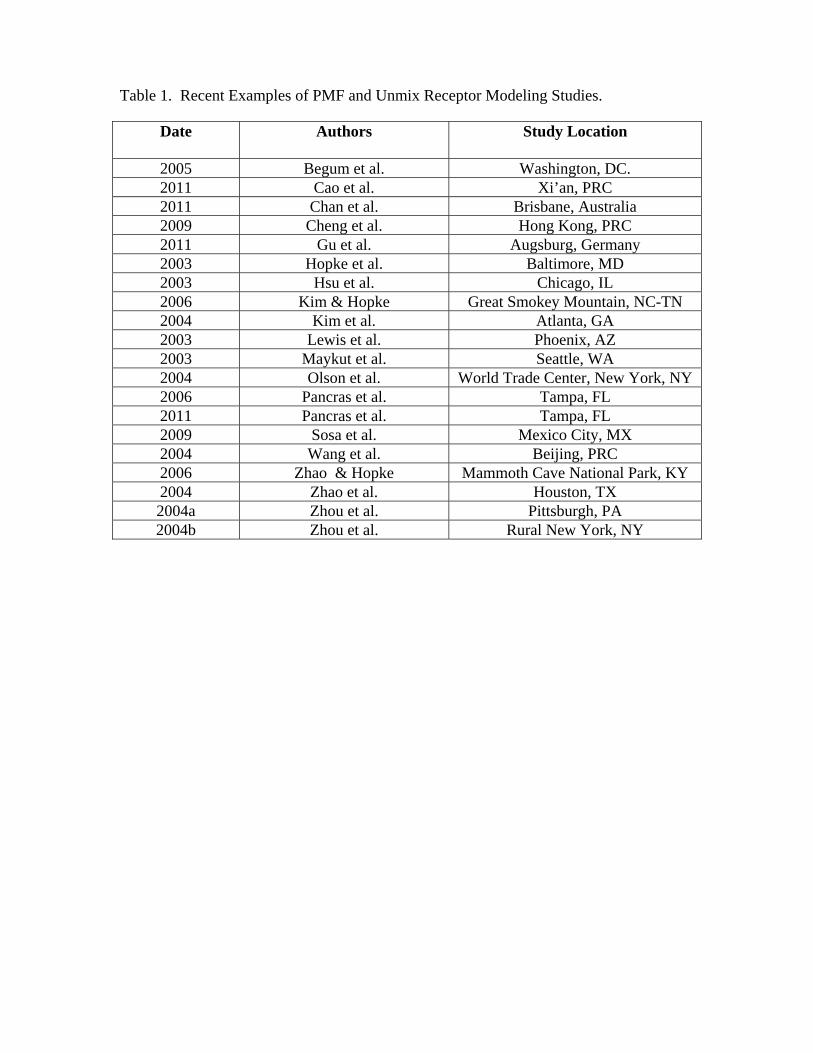
Table 1. Recent Examples of PMF and Unmix Receptor Modeling Studies.
Date Authors Study Location
2005 Begum et al. Washington, DC. 2011 Cao et al. Xi’an, PRC 2011 Chan et al. Brisbane, Australia 2009 Cheng et al. Hong Kong, PRC 2011 Gu et al. Augsburg, Germany 2003 Hopke et al. Baltimore, MD 2003 Hsu et al. Chicago, IL 2006 Kim & Hopke Great Smokey Mountain, NC-TN 2004 Kim et al. Atlanta, GA 2003 Lewis et al. Phoenix, AZ 2003 Maykut et al. Seattle, WA 2004 Olson et al. World Trade Center, New York, NY 2006 Pancras et al. Tampa, FL 2011 Pancras et al. Tampa, FL 2009 Sosa et al. Mexico City, MX 2004 Wang et al. Beijing, PRC 2006 Zhao & Hopke Mammoth Cave National Park, KY 2004 Zhao et al. Houston, TX 2004a Zhou et al. Pittsburgh, PA 2004b Zhou et al. Rural New York, NY
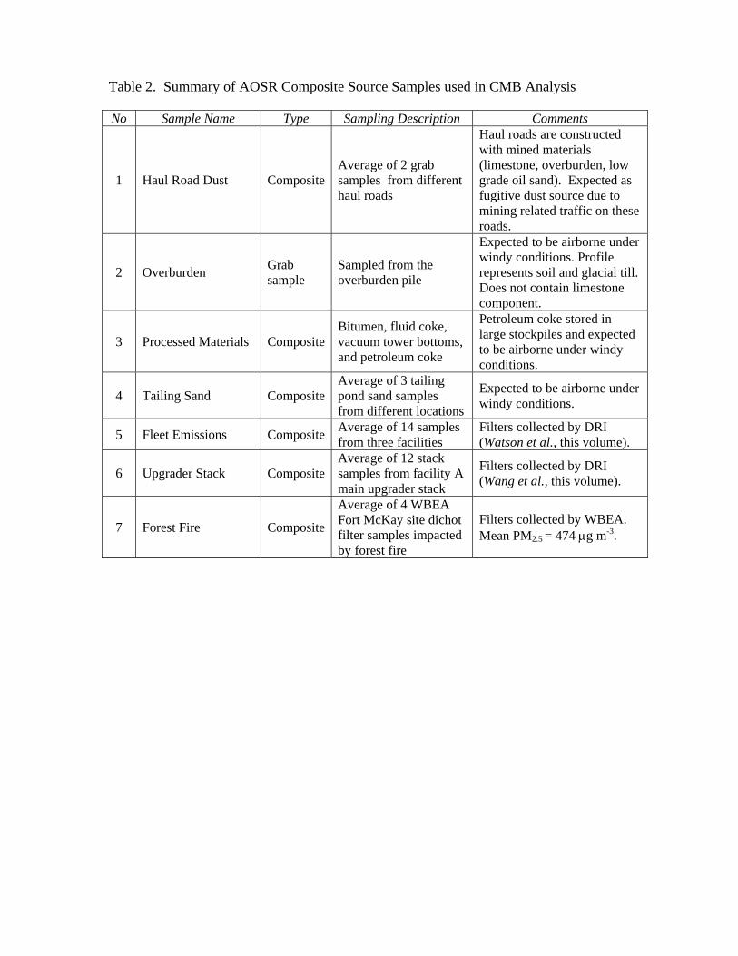
Table 2. Summary of AOSR Composite Source Samples used in CMB Analysis No Sample Name Type Sampling Description Comments
1 Haul Road Dust CompositeAverage of 2 grab samples from different haul roads
Haul roads are constructed with mined materials (limestone, overburden, low grade oil sand). Expected as fugitive dust source due to mining related traffic on these roads.
2 Overburden Grab sample
Sampled from the overburden pile
Expected to be airborne under windy conditions. Profile represents soil and glacial till. Does not contain limestone component.
3 Processed Materials CompositeBitumen, fluid coke, vacuum tower bottoms, and petroleum coke
Petroleum coke stored in large stockpiles and expected to be airborne under windy conditions.
4 Tailing Sand CompositeAverage of 3 tailing pond sand samples from different locations
Expected to be airborne under windy conditions.
5 Fleet Emissions CompositeAverage of 14 samples from three facilities
Filters collected by DRI (Watson et al., this volume).
6 Upgrader Stack CompositeAverage of 12 stack samples from facility A main upgrader stack
Filters collected by DRI (Wang et al., this volume).
7 Forest Fire Composite
Average of 4 WBEA Fort McKay site dichot filter samples impacted by forest fire
Filters collected by WBEA. Mean PM2.5 = 474 g m-3.
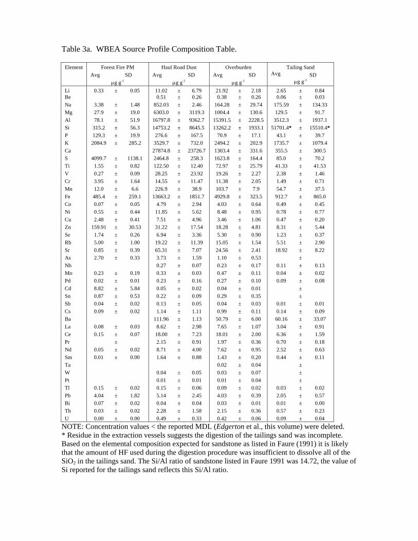
Table 3a. WBEA Source Profile Composition Table.
Element Forest Fire PM Haul Road Dust Overburden
Tailing Sand
Avg SD Avg SD Avg SD Avg SD
g g-1 g g-1 g g-1 g g-1
Li 0.33 ± 0.05 11.02 ± 6.79 21.92 ± 2.18 2.65 ± 0.84 Be 0.51 ± 0.26 0.38 ± 0.26 0.06 ± 0.03
Na 3.38 ± 1.48 852.03 ± 2.46 164.28 ± 29.74 175.59 ± 134.33
Mg 27.9 ± 19.0 6303.0 ± 3119.3 1004.4 ± 130.6 129.5 ± 91.7
Al 78.1 ± 51.9 16797.8 ± 9362.7 15391.5 ± 2228.5 3512.3 ± 1937.1
Si 315.2 ± 56.3 14753.2 ± 8645.5 13262.2 ± 1933.1 51701.4* ± 15510.4*
P 129.3 ± 19.9 276.6 ± 167.5 70.9 ± 17.1 43.1 ± 39.7
K 2084.9 ± 285.2 3529.7 ± 732.0 2494.2 ± 202.9 1735.7 ± 1079.4
Ca 27874.8 ± 23726.7 1303.4 ± 331.6 355.5 ± 300.5
S 4099.7 ± 1138.1 2464.8 ± 258.3 1623.8 ± 164.4 85.0 ± 70.2
Ti 1.55 ± 0.82 122.50 ± 12.40 72.97 ± 25.79 41.33 ± 41.53
V 0.27 ± 0.09 28.25 ± 23.92 19.26 ± 2.27 2.38 ± 1.46
Cr 3.95 ± 1.64 14.55 ± 11.47 11.38 ± 2.05 1.49 ± 0.71
Mn 12.0 ± 6.6 226.9 ± 38.9 103.7 ± 7.9 54.7 ± 37.5
Fe 485.4 ± 259.1 13663.2 ± 1851.7 4929.8 ± 323.5 912.7 ± 865.0
Co 0.07 ± 0.05 4.79 ± 2.94 4.03 ± 0.64 0.49 ± 0.45
Ni 0.55 ± 0.44 11.85 ± 5.62 8.48 ± 0.95 0.78 ± 0.77
Cu 2.48 ± 0.41 7.51 ± 4.96 3.46 ± 1.06 0.47 ± 0.20
Zn 159.91 ± 30.53 31.22 ± 17.54 18.28 ± 4.81 8.31 ± 5.44
Se 1.74 ± 0.26 6.94 ± 3.36 5.30 ± 0.90 1.23 ± 0.37
Rb 5.00 ± 1.00 19.22 ± 11.39 15.05 ± 1.54 5.51 ± 2.90
Sr 0.85 ± 0.39 65.31 ± 7.07 24.56 ± 2.41 18.92 ± 8.22
As 2.70 ± 0.33 3.73 ± 1.59 1.10 ± 0.53 ±
Nb 0.27 ± 0.07 0.23 ± 0.17 0.11 ± 0.13
Mo 0.23 ± 0.19 0.33 ± 0.03 0.47 ± 0.11 0.04 ± 0.02
Pd 0.02 ± 0.01 0.23 ± 0.16 0.27 ± 0.10 0.09 ± 0.08
Cd 8.82 ± 5.84 0.05 ± 0.02 0.04 ± 0.01 ±
Sn 0.87 ± 0.53 0.22 ± 0.09 0.29 ± 0.35 ±
Sb 0.04 ± 0.02 0.13 ± 0.05 0.04 ± 0.03 0.01 ± 0.01
Cs 0.09 ± 0.02 1.14 ± 1.11 0.99 ± 0.11 0.14 ± 0.09
Ba 111.96 ± 1.13 50.79 ± 6.00 60.16 ± 33.07
La 0.08 ± 0.03 8.62 ± 2.98 7.65 ± 1.07 3.04 ± 0.91
Ce 0.15 ± 0.07 18.00 ± 7.23 18.01 ± 2.00 6.36 ± 1.59
Pr ± 2.15 ± 0.91 1.97 ± 0.36 0.70 ± 0.18
Nd 0.05 ± 0.02 8.71 ± 4.00 7.62 ± 0.95 2.52 ± 0.63
Sm 0.01 ± 0.00 1.64 ± 0.88 1.43 ± 0.20 0.44 ± 0.11
Ta 0.02 ± 0.04 ±
W 0.04 ± 0.05 0.03 ± 0.07 ±
Pt 0.01 ± 0.01 0.01 ± 0.04 ±
Tl 0.15 ± 0.02 0.15 ± 0.06 0.09 ± 0.02 0.03 ± 0.02
Pb 4.04 ± 1.82 5.14 ± 2.45 4.03 ± 0.39 2.05 ± 0.57
Bi 0.07 ± 0.02 0.04 ± 0.04 0.03 ± 0.01 0.01 ± 0.00
Th 0.03 ± 0.02 2.28 ± 1.58 2.15 ± 0.36 0.57 ± 0.23
U 0.00 ± 0.00 0.49 ± 0.33 0.42 ± 0.06 0.09 ± 0.04
NOTE: Concentration values < the reported MDL (Edgerton et al., this volume) were deleted. * Residue in the extraction vessels suggests the digestion of the tailings sand was incomplete. Based on the elemental composition expected for sandstone as listed in Faure (1991) it is likely that the amount of HF used during the digestion procedure was insufficient to dissolve all of the SiO2 in the tailings sand. The Si/Al ratio of sandstone listed in Faure 1991 was 14.72, the value of Si reported for the tailings sand reflects this Si/Al ratio.
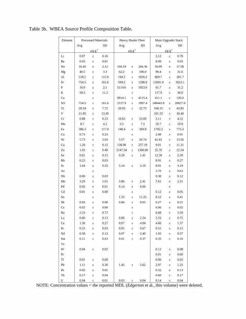
Table 3b. WBEA Source Profile Composition Table.
Element Processed Materials Heavy Hauler Fleet Main Upgrader Stack
Avg SD Avg SD Avg SD
g g-1 g g-1 g g-1
Li 0.97 ± 0.16 3.12 ± 0.78
Be 0.03 ± 0.01 0.09 ± 0.03
Na 16.45 ± 2.12 104.19 ± 266.36 56.09 ± 17.58
Mg 40.5 ± 3.3 62.2 ± 106.0 90.4 ± 31.6
Al 518.1 ± 112.9 194.2 ± 1826.2 809.7 ± 281.7
Si 754.5 ± 161.6 594.2 ± 1286.0 12691.0 ± 3623.1
P 10.9 ± 2.1 5114.6 ± 1923.6 61.7 ± 31.2
K 58.3 ± 11.2 ± 117.9 ± 36.0
Ca ± 9914.1 ± 4115.4 411.1 ± 120.0
SO 754.5 ± 161.6 2157.9 ± 1897.4 148443.8 ± 20627.0
Ti 28.54 ± 7.72 20.92 ± 32.75 168.15 ± 43.85
V 21.85 ± 13.30 101.55 ± 30.40
Cr 0.88 ± 0.23 10.65 ± 33.69 3.11 ± 4.52
Mn 8.7 ± 4.2 3.3 ± 7.5 50.7 ± 19.9
Fe 386.3 ± 117.0 148.4 ± 369.8 1792.2 ± 773.3
Co 0.73 ± 0.23 ± 2.68 ± 0.91
Ni 5.73 ± 2.03 5.57 ± 20.74 41.82 ± 15.56
Cu 1.26 ± 0.15 138.06 ± 257.18 9.01 ± 11.31
Zn 1.93 ± 0.40 5147.34 ± 1300.00 25.70 ± 22.54
Se 0.61 ± 0.15 0.29 ± 1.41 12.30 ± 2.59
Rb 0.23 ± 0.03 0.91 ± 0.27
Sr 1.64 ± 0.35 5.14 ± 3.19 8.91 ± 3.19
As ± 3.70 ± 0.63
Nb 0.06 ± 0.03 0.38 ± 0.12
Mo 3.29 ± 1.01 3.86 ± 2.41 7.61 ± 2.51
Pd 0.02 ± 0.01 0.14 ± 0.66 ±
Cd 0.01 ± 0.00 ± 0.12 ± 0.05
Sn ± 1.33 ± 11.25 0.53 ± 0.41
Sb 0.02 ± 0.00 0.84 ± 9.05 0.27 ± 0.21
Cs 0.02 ± 0.00 ± 0.06 ± 0.02
Ba 2.23 ± 0.72 ± 6.68 ± 3.59
La 0.60 ± 0.13 0.06 ± 2.24 2.55 ± 0.75
Ce 1.30 ± 0.27 0.07 ± 4.94 4.60 ± 1.37
Pr 0.15 ± 0.03 0.05 ± 0.67 0.51 ± 0.15
Nd 0.58 ± 0.13 0.07 ± 2.40 1.92 ± 0.57
Sm 0.11 ± 0.03 0.01 ± 0.37 0.35 ± 0.10
Ta
W 0.04 ± 0.02 0.12 ± 0.08
Pt 0.01 ± 0.00
Tl 0.01 ± 0.00 0.06 ± 0.02
Pb 1.11 ± 0.30 1.45 ± 5.02 2.97 ± 1.25
Bi 0.02 ± 0.01 0.32 ± 0.13
Th 0.17 ± 0.04 0.60 ± 0.17
U 0.04 ± 0.01 0.03 ± 0.04 0.14 ± 0.04
NOTE: Concentration values < the reported MDL (Edgerton et al., this volume) were deleted.
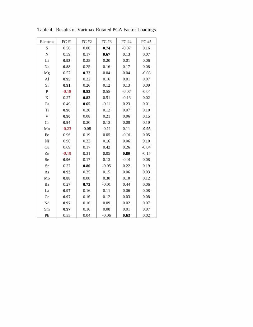
Table 4. Results of Varimax Rotated PCA Factor Loadings.
Element FC #1 FC #2 FC #3 FC #4 FC #5
S 0.50 0.00 0.74 -0.07 0.16
N 0.59 0.17 0.67 0.13 0.07
Li 0.93 0.25 0.20 0.01 0.06
Na 0.88 0.25 0.16 0.17 0.08
Mg 0.57 0.72 0.04 0.04 -0.08
Al 0.95 0.22 0.16 0.01 0.07
Si 0.91 0.26 0.12 0.13 0.09
P -0.18 0.82 0.55 -0.07 -0.04
K 0.27 0.82 0.51 -0.13 0.02
Ca 0.49 0.65 -0.11 0.23 0.01
Ti 0.96 0.20 0.12 0.07 0.10
V 0.90 0.08 0.21 0.06 0.15
Cr 0.94 0.20 0.13 0.08 0.10
Mn -0.23 -0.08 -0.11 0.11 -0.95
Fe 0.96 0.19 0.05 -0.01 0.05
Ni 0.90 0.23 0.16 0.06 0.10
Cu 0.69 0.17 0.42 0.26 -0.04
Zn -0.19 0.31 0.05 0.80 -0.15
Se 0.96 0.17 0.13 -0.01 0.08
Sr 0.27 0.80 -0.05 0.22 0.19
As 0.93 0.25 0.15 0.06 0.03
Mo 0.88 0.08 0.30 0.10 0.12
Ba 0.27 0.72 -0.01 0.44 0.06
La 0.97 0.16 0.11 0.06 0.08
Ce 0.97 0.16 0.12 0.03 0.08
Nd 0.97 0.16 0.09 0.02 0.07
Sm 0.97 0.16 0.08 0.01 0.07
Pb 0.55 0.04 -0.06 0.63 0.02
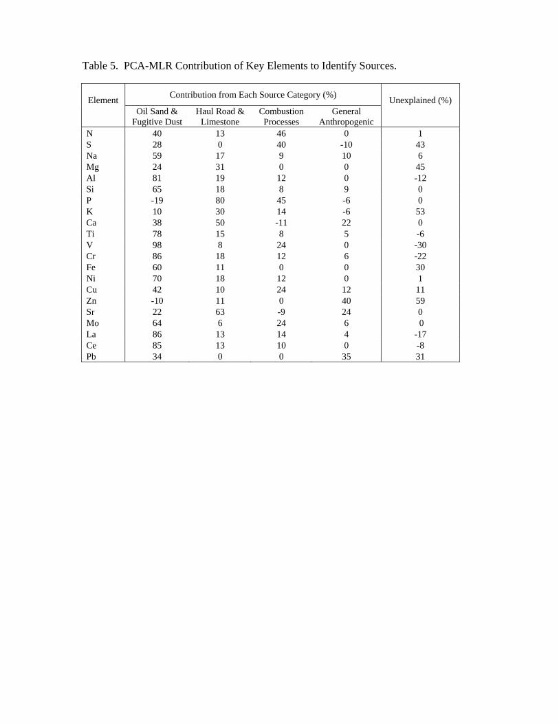
Table 5. PCA-MLR Contribution of Key Elements to Identify Sources.
Element
Contribution from Each Source Category (%) Unexplained (%)
Oil Sand & Fugitive Dust
Haul Road & Limestone
Combustion Processes
General Anthropogenic
N 40 13 46 0 1 S 28 0 40 -10 43 Na 59 17 9 10 6 Mg 24 31 0 0 45 Al 81 19 12 0 -12 Si 65 18 8 9 0 P -19 80 45 -6 0 K 10 30 14 -6 53 Ca 38 50 -11 22 0 Ti 78 15 8 5 -6 V 98 8 24 0 -30 Cr 86 18 12 6 -22 Fe 60 11 0 0 30 Ni 70 18 12 0 1 Cu 42 10 24 12 11 Zn -10 11 0 40 59 Sr 22 63 -9 24 0 Mo 64 6 24 6 0 La 86 13 14 4 -17 Ce 85 13 10 0 -8 Pb 34 0 0 35 31
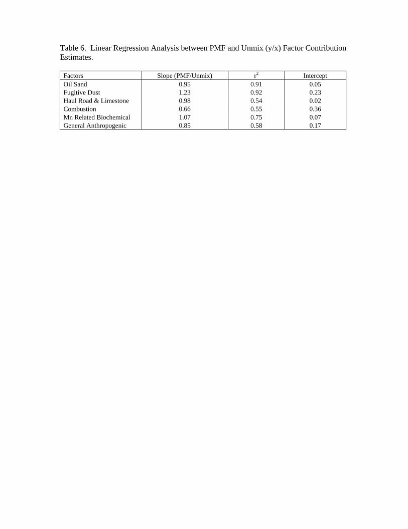
Table 6. Linear Regression Analysis between PMF and Unmix (y/x) Factor Contribution Estimates.
Factors Slope (PMF/Unmix) r2 Intercept Oil Sand 0.95 0.91 0.05 Fugitive Dust 1.23 0.92 0.23 Haul Road & Limestone 0.98 0.54 0.02 Combustion 0.66 0.55 0.36 Mn Related Biochemical 1.07 0.75 0.07 General Anthropogenic 0.85 0.58 0.17
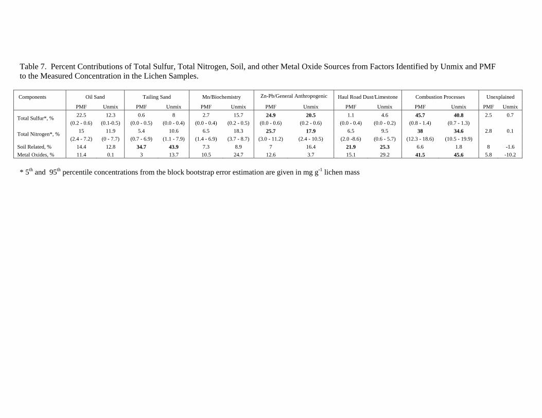
Table 7. Percent Contributions of Total Sulfur, Total Nitrogen, Soil, and other Metal Oxide Sources from Factors Identified by Unmix and PMF to the Measured Concentration in the Lichen Samples.
Components Oil Sand Tailing Sand Mn/Biochemistry
Zn-Pb/General Anthropogenic Haul Road Dust/Limestone Combustion Processes Unexplained
PMF Unmix PMF Unmix PMF Unmix PMF Unmix PMF Unmix PMF Unmix PMF Unmix
Total Sulfur*, % 22.5 12.3 0.6 8 2.7 15.7 24.9 20.5 1.1 4.6 45.7 40.8 2.5 0.7
(0.2 - 0.6) (0.1-0.5) (0.0 - 0.5) (0.0 - 0.4) (0.0 - 0.4) (0.2 - 0.5) (0.0 - 0.6) (0.2 - 0.6) (0.0 - 0.4) (0.0 - 0.2) (0.8 - 1.4) (0.7 - 1.3)
Total Nitrogen*, % 15 11.9 5.4 10.6 6.5 18.3 25.7 17.9 6.5 9.5 38 34.6 2.8 0.1
(2.4 - 7.2) (0 - 7.7) (0.7 - 6.9) (1.1 - 7.9) (1.4 - 6.9) (3.7 - 8.7) (3.0 - 11.2) (2.4 - 10.5) (2.0 -8.6) (0.6 - 5.7) (12.3 - 18.6) (10.5 - 19.9)
Soil Related, % 14.4 12.8 34.7 43.9 7.3 8.9 7 16.4 21.9 25.3 6.6 1.8 8 -1.6
Metal Oxides, % 11.4 0.1 3 13.7 10.5 24.7 12.6 3.7 15.1 29.2 41.5 45.6 5.8 -10.2
* 5th and 95th percentile concentrations from the block bootstrap error estimation are given in mg g-1 lichen mass
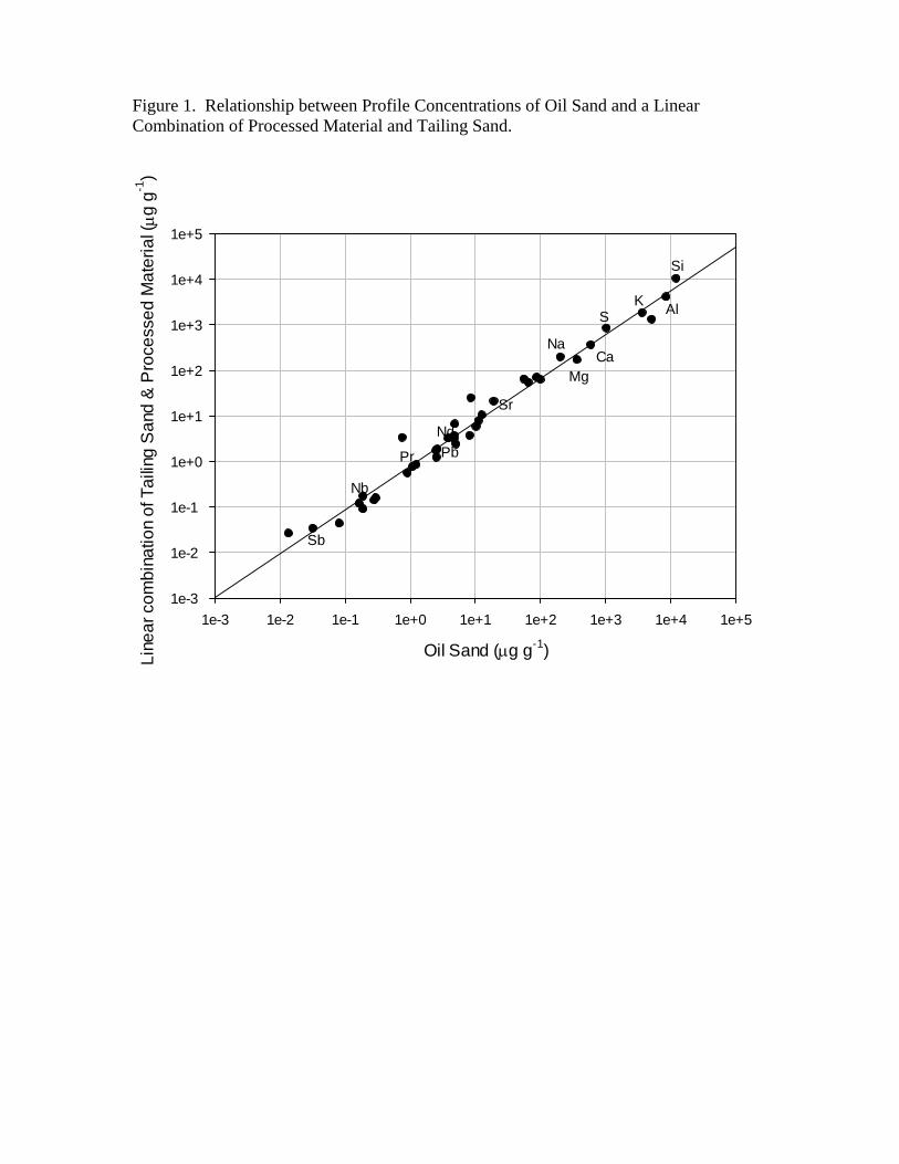
Figure 1. Relationship between Profile Concentrations of Oil Sand and a Linear Combination of Processed Material and Tailing Sand.
Oil Sand (g g-1)
1e-3 1e-2 1e-1 1e+0 1e+1 1e+2 1e+3 1e+4 1e+5
Lin
ea
r co
mb
ina
tion
of T
aili
ng S
and
& P
roce
sse
d M
ate
ria
l (g
g-1
)
1e-3
1e-2
1e-1
1e+0
1e+1
1e+2
1e+3
1e+4
1e+5
Pr
Nd
Mg
Sr
Na
S
Ca
KAl
Si
Nb
Sb
Pb
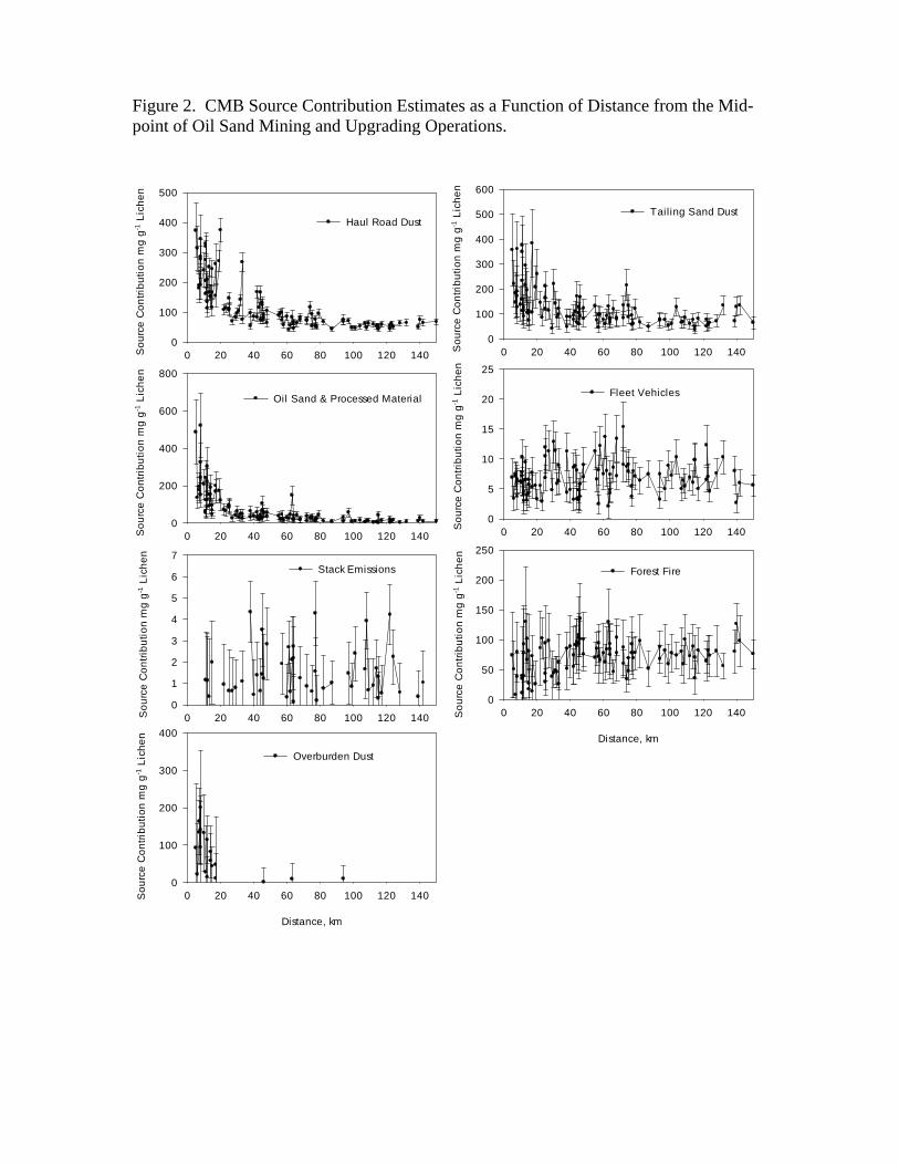
Figure 2. CMB Source Contribution Estimates as a Function of Distance from the Mid-point of Oil Sand Mining and Upgrading Operations.
Distance, km
0 20 40 60 80 100 120 140So
urc
e C
on
trib
uti
on
mg
g-1
Lic
he
n
0
100
200
300
400
500
Haul Road Dust
Distance, km
0 20 40 60 80 100 120 140So
urc
e C
on
trib
uti
on
mg
g-1
Lic
he
n
0
100
200
300
400
500
600
Tailing Sand Dust
Distance, km
0 20 40 60 80 100 120 140So
urc
e C
on
trib
uti
on
mg
g-1
Lic
he
n
0
200
400
600
800
Oil Sand & Processed Material
Distance, km
0 20 40 60 80 100 120 140So
urc
e C
on
trib
uti
on
mg
g-1
Lic
he
n
0
5
10
15
20
25
Fleet Vehicles
Distance, km
0 20 40 60 80 100 120 140So
urc
e C
on
trib
uti
on
mg
g-1
Lic
he
n
0
1
2
3
4
5
6
7Stack Emissions
Distance, km
0 20 40 60 80 100 120 140So
urc
e C
on
trib
uti
on
mg
g-1
Lic
he
n
0
50
100
150
200
250
Forest Fire
Distance, km
0 20 40 60 80 100 120 140So
urc
e C
on
trib
uti
on
mg
g-1
Lic
he
n
0
100
200
300
400
Overburden Dust
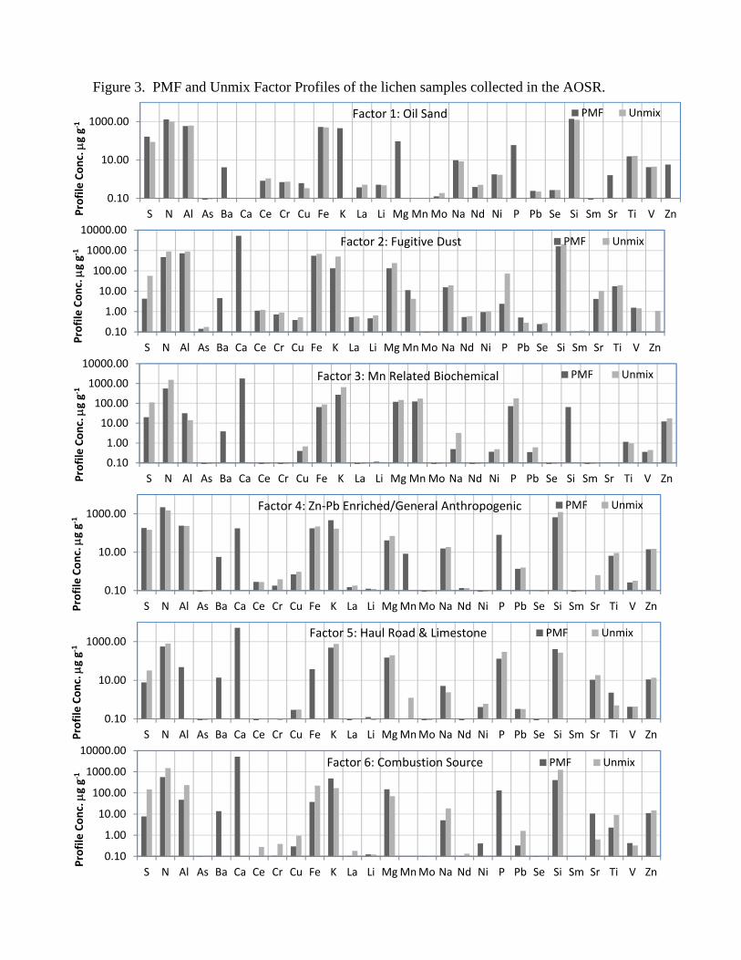
Figure 3. PMF and Unmix Factor Profiles of the lichen samples collected in the AOSR.
0.10
10.00
1000.00
S N Al As Ba Ca Ce Cr Cu Fe K La Li Mg MnMo Na Nd Ni P Pb Se Si Sm Sr Ti V ZnProfile Conc. g g‐
1
PMF UnmixFactor 1: Oil Sand
0.10
1.00
10.00
100.00
1000.00
10000.00
S N Al As Ba Ca Ce Cr Cu Fe K La Li MgMnMo Na Nd Ni P Pb Se Si Sm Sr Ti V Zn
Profile Conc. g g‐
1
PMF UnmixFactor 2: Fugitive Dust
0.10
1.00
10.00
100.00
1000.00
10000.00
S N Al As Ba Ca Ce Cr Cu Fe K La Li Mg MnMo Na Nd Ni P Pb Se Si Sm Sr Ti V ZnProfile Conc. g g‐
1
PMF UnmixFactor 3: Mn Related Biochemical
0.10
10.00
1000.00
S N Al As Ba Ca Ce Cr Cu Fe K La Li MgMnMo Na Nd Ni P Pb Se Si Sm Sr Ti V ZnProfile Conc. g g‐
1
PMF UnmixFactor 4: Zn‐Pb Enriched/General Anthropogenic
0.10
10.00
1000.00
S N Al As Ba Ca Ce Cr Cu Fe K La Li MgMnMo Na Nd Ni P Pb Se Si Sm Sr Ti V ZnProfile Conc. g g‐
1
PMF UnmixFactor 5: Haul Road & Limestone
0.10
1.00
10.00
100.00
1000.00
10000.00
S N Al As Ba Ca Ce Cr Cu Fe K La Li MgMnMo Na Nd Ni P Pb Se Si Sm Sr Ti V Zn
Profile Conc. g g‐
1
PMF UnmixFactor 6: Combustion Source
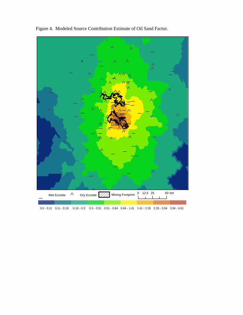
Figure 4. Modeled Source Contribution Estimate of Oil Sand Factor.
0.0 - 0.11 0.11 - 0.19 0.19 - 0.3 0.3 - 0.51 0.51 - 0.84 0.84 - 1.41 1.41 - 2.35 2.35 - 3.94 3.94 - 6.61
_ Wet Ecosite ^ Dry Ecosite Mining Footprint 0 25 5012.5 km
__̂
_
^ ___̂
^_^
_^
_ __̂
^
^
^
^
^
^ ^̂^
^__
__^
^ ^_
^
^^__
^_
_
_̂^
^
_
^^
_
^
_
^
_^
^
^
^
^
_
_
_
_
^_
^
^
_
^
_
_
_
_
_^
_
_
_^
_
_
^
^
^
^
^
_
_
_
^
^
_
^
^
_
^_
^
_
^
^
_ ^
_
^
_
_
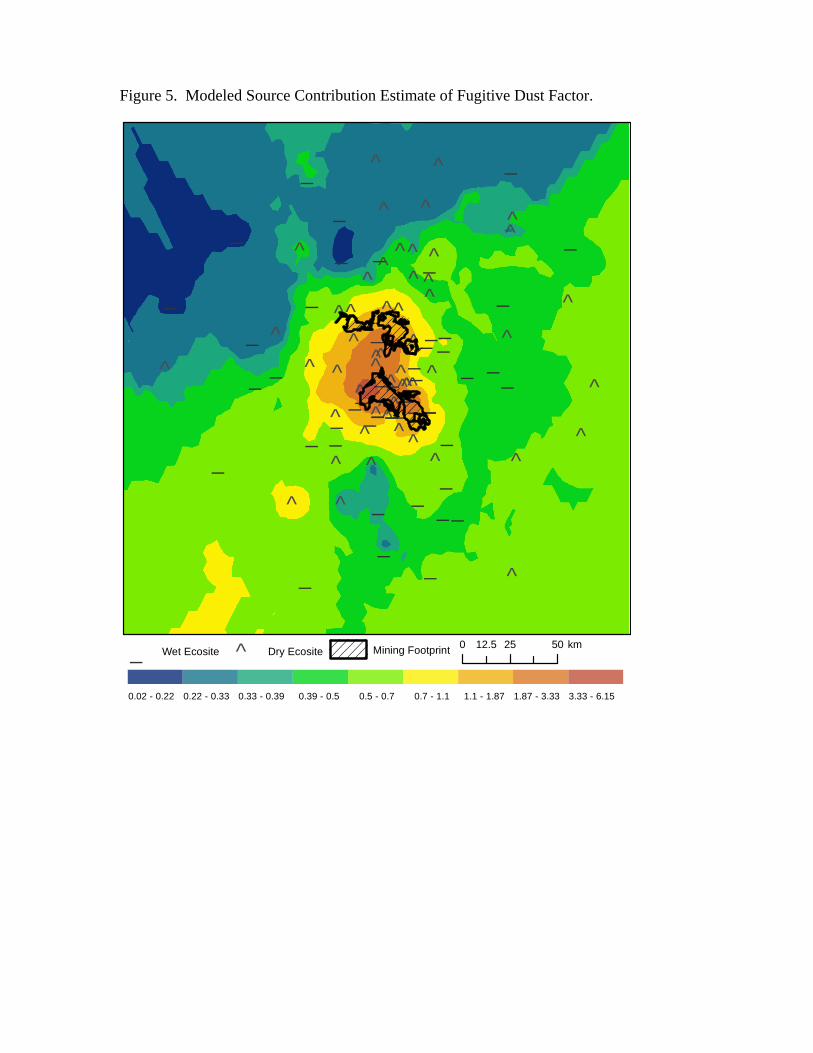
Figure 5. Modeled Source Contribution Estimate of Fugitive Dust Factor.
0.02 - 0.22 0.22 - 0.33 0.33 - 0.39 0.39 - 0.5 0.5 - 0.7 0.7 - 1.1 1.1 - 1.87 1.87 - 3.33 3.33 - 6.15
_ Wet Ecosite ^ Dry Ecosite Mining Footprint 0 25 5012.5 km
__̂
_
^ ___̂
^_^
_^
_ __̂
^
^
^
^
^
^ ^̂^
^__
__^
^ ^_
^
^^__
^_
_
_̂^
^
_
^^
_
^
_
^
_^
^
^
^
^
_
_
_
_
^_
^
^
_
^
_
_
_
_
_^
_
_
_^
_
_
^
^
^
^
^
_
_
_
^
^
_
^
^
_
^_
^
_
^
^
_ ^
_
^
_
_
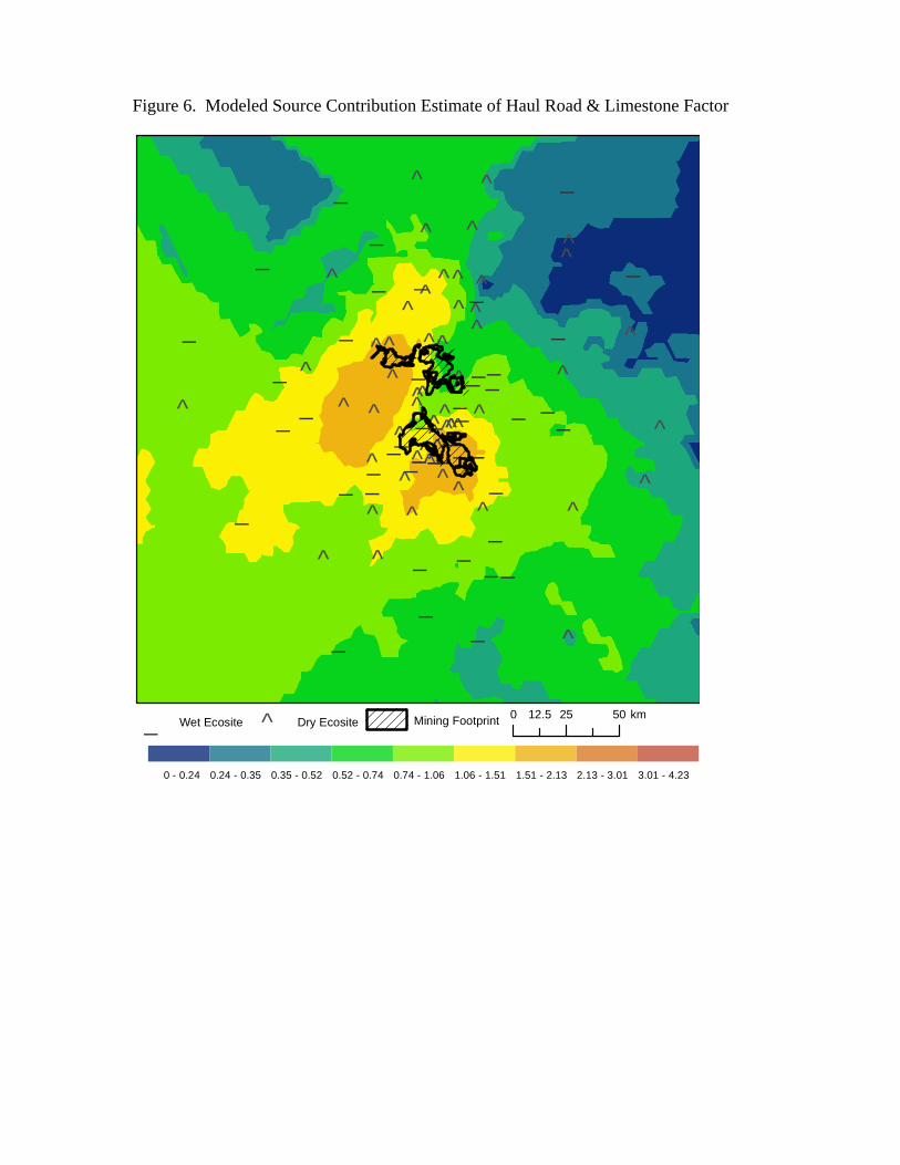
Figure 6. Modeled Source Contribution Estimate of Haul Road & Limestone Factor
0 - 0.24 0.24 - 0.35 0.35 - 0.52 0.52 - 0.74 0.74 - 1.06 1.06 - 1.51 1.51 - 2.13 2.13 - 3.01 3.01 - 4.23
_ Wet Ecosite ^ Dry Ecosite Mining Footprint 0 25 5012.5 km
__̂
_
^ ___̂
^_^
_^
_ __̂
^
^
^
^
^
^ ^̂^
^__
__^
^ ^_
^
^^__
^_
_
_̂^
^
_
^^
_
^
_
^
_^
^
^
^
^
_
_
_
_
^_
^
^
_
^
_
_
_
_
_^
_
_
_^
_
_
^
^
^
^
^
_
_
_
^
^
_
^
^
_
^_
^
_
^
^
_ ^
_
^
_
_

Figure 7. Modeled Source Contribution Estimate of Combustion Source Factor.
Mining Footprint_ Wet Ecosite ^ Dry Ecosite
0.0 - 0.27 0.27 - 0.57 0.57 - 0.8 0.8 - 0.98 0.98 - 1.21 1.21 - 1.51 1.51 - 1.9 1.9 - 2.42 2.42 - 3.09
²0 20 4010 km
__̂
_
^ ___̂
^_^
_
^_ __̂
^
^
^
^
^
^ ^̂^
^_
__
_^
^ ^
_
^
^^_
_^
_
_
_̂^
^
_
^^
_
^
_
^
_
^
^
^
^
^
_
_
_
_
^_
^
^
_
^
_
_
_
_
_
^
_
_
_^
_
_
^
^
^
^
^
_
_
_
^
^
_
^
^
_
^_
^
_
^
_ ^
_
^
_
_
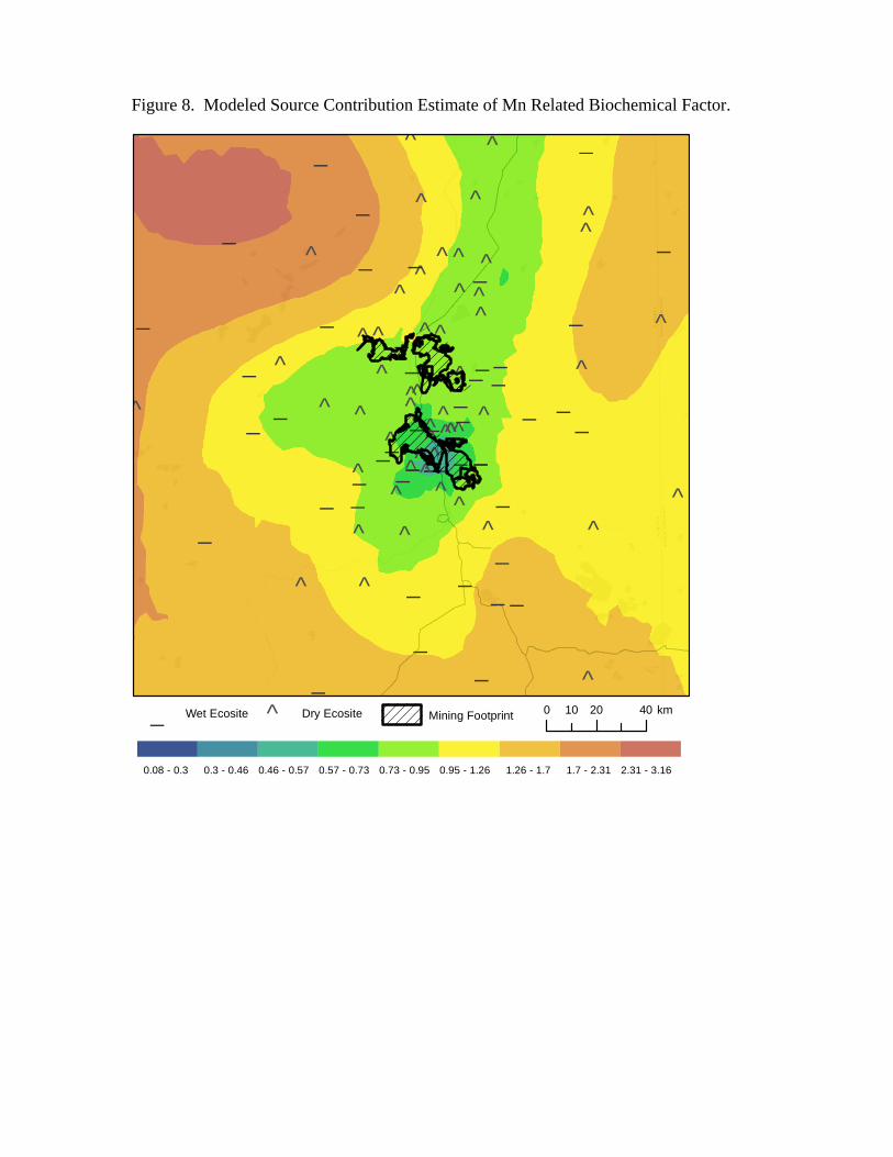
Figure 8. Modeled Source Contribution Estimate of Mn Related Biochemical Factor.
0.08 - 0.3 0.3 - 0.46 0.46 - 0.57 0.57 - 0.73 0.73 - 0.95 0.95 - 1.26 1.26 - 1.7 1.7 - 2.31 2.31 - 3.16
Mining Footprint_ Wet Ecosite ^ Dry Ecosite
²0 20 4010 km
__̂
_
^ ___̂
^_^
_
^_ __̂
^
^
^
^
^
^ ^̂^
^_
__
_^
^ ^
_
^
^^_
_^
_
_
_̂^
^
_
^^
_
^
_
^
_
^
^
^
^
^
_
_
_
_
^_
^
^
_
^
_
_
_
_
_
^
_
_
_^
_
_
^
^
^
^
^
_
_
_
^
^
_
^
^
_
^_
^
_
^
_ ^
_
^
_
_
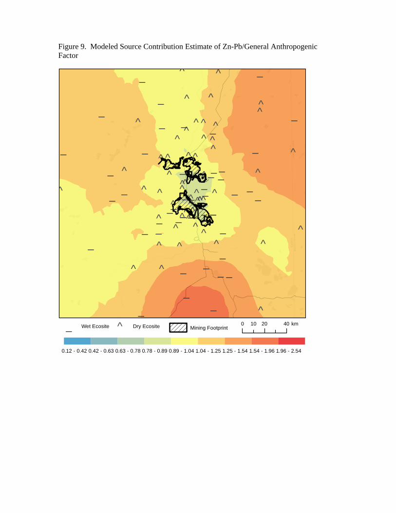
Figure 9. Modeled Source Contribution Estimate of Zn-Pb/General Anthropogenic Factor
_ Wet Ecosite ^ Dry Ecosite Mining Footprint
0.12 - 0.42 0.42 - 0.63 0.63 - 0.78 0.78 - 0.89 0.89 - 1.04 1.04 - 1.25 1.25 - 1.54 1.54 - 1.96 1.96 - 2.54
²0 20 4010 km
__̂
_
^ ___̂
^_^
_
^_ __̂
^
^
^
^
^
^ ^̂^
^_
__
_^
^ ^
_
^
^^_
_^
_
_
_̂^
^
_
^^
_
^
_
^
_
^
^
^
^
^
_
_
_
_
^_
^
^
_
^
_
_
_
_
_
^
_
_
_^
_
_
^
^
^
^
^
_
_
_
^
^
_
^
^
_
^_
^
_
^
_ ^
_
^
_
_
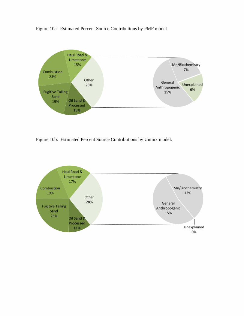
Figure 10a. Estimated Percent Source Contributions by PMF model.
Figure 10b. Estimated Percent Source Contributions by Unmix model.
Oil Sand &Processed
15%
Fugitive Tailing Sand19%
Combustion23%
Haul Road & Limestone
15%
General Anthropogenic
15%
Mn/Biochemistry7%
Unexplained6%
Other28%
Oil Sand &Processed
11%
Fugitive Tailing Sand25%
Combustion19%
Haul Road & Limestone
17%
General Anthropogenic
15%
Mn/Biochemistry13%
Unexplained0%
Other28%