Chapter 2 Filter Banks and DWT

Chapter 2Filter Banks and DWT

Abstract The study of digital signal processing normally concentrates on thedesign, realization, and application of single-input, single-output digital filters.There are applications, as in the case of spectrum analyzer, where it is desired toseparate a signal into a set of sub-band signals occupying, usually nonoverlapping,portions of the original frequency band. In other applications, it may be desired tocombine many such sub-band signals into a single composite signal occupying thewhole Nyquist range. To this end, digital filter banks play an important role.Implementation of a filter bank on a processor with finite precision arithmeticnecessitates quantization of filter coefficients [95]. This results in loss of perfectreconstruction (PR) property. The theory offilter banks were developed much beforemodern discrete wavelet transform (DWT) analysis became popular [127, 134]. Thestudy of literature reveals a close relationship between the DWT and digital filterbanks. It turns out that a tree of digital filter banks, without computing motherwavelets, can simply achieve the wavelet transform. Hence, the filter banks havebeen playing a central role in the area of wavelet analysis. It is therefore of interest tostudy the filter bank theory before addressing the implementation issues of finiteprecision wavelet transforms. In this chapter, fundamental concept of filter banktheory leading to new implementation issues described in latter chapters is intro-duced. The material presented in this chapter will be useful in discussing errormodeling and parallel computing techniques discussed in the book. In presentchapter, the filter bank concept related to DWT is revisited in Sect. 2.1. Section 2.2presents two-channel PR filter bank. Section 2.3 presents derivation of parallel filterDWT from pyramid DWT structure. Section 2.4 presents frequency response ofgenerated parallel filters followed by conclusion in Sect. 2.5.

Keywords Filter banks � Quantum mirror filter � Aliasing � Computationcomplexity

K. K. Shukla and A. K. Tiwari, Efficient Algorithms for Discrete Wavelet Transform,SpringerBriefs in Computer Science, DOI: 10.1007/978-1-4471-4941-5_2,� K. K. Shukla 2013

21

2.1 Introduction

In the classical applications of multirate filter banks, a bank of analysis filters isapplied to a discrete input signal and then down sampled at fixed rate to produce aset of sub-band signals. If a dual bank of synthesis filters exists, by means of whichthe original input signal can be recovered by first upsampling each of the abovesub-band signals and then applying it to a synthesis filter, then the two filter banksare said to be a perfect reconstruction (PR) pair of filter banks [113]. The termuniform filter bank (UFB) is used to emphasize that all the sub-band signals aredownsampled at the same rate [125]. PR pair of wavelet analysis and synthesisfilter banks is dual. The discrete wavelet transform (DWT), and multiresolutionanalysis, can be viewed as the application of a nonuniform filter bank, defined by aUFB. In terms of wavelet theory, a low-pass filter corresponds to scaling functionand the subsequent high-pass or band-pass filter corresponds to wavelet function.The DWT computation involves repetitive application of UFB on the low-passchannel. In the literatures, wavelet transform have been treated in considerabledetail and wavelet decompositions have been related to PR Filter Bank [35, 132,134, 139].

The concept of PR is meaningful only in the ideal cases. In most real worldapplications of finite world length, some sort of error is always introduced in thecoding process or during the transmission over lossy channels. The advantage ofmultiresolution scheme is that the redundancy is introduced more in low-frequencychannels compared to high-frequency channels. Thus, these representations maybe advantageous for certain classes of signals such as natural images.

2.2 Orthogonal Filter Banks

The digital filter bank is defined as a set of digital band-pass filters with either acommon input or a summed output and is referred as analysis and synthesis filterbank, respectively. The operation of analysis and synthesis filter bank is dual toeach other. The combined structure of analysis and synthesis filter bank is quad-rature mirror filter (QMF) bank [113].

Process of filtering is usually related with frequency selectivity. For example,an ideal discrete-time low-pass filter with cutoff frequency xc \ p takes any inputsignal and projects it onto the subspace of signals bandlimited to [-xc, xc].Orthogonal discrete-time filter banks perform a similar projection. Assume adiscrete-time filter with finite impulse response gg½n� ¼ fgg½0�; gg½1�; . . .; gg½L� g;L even, and the property [107]

hgg½n�; gg½n � 2k�i ¼ dk ð2:1Þ

22 2 Filter Banks and DWT

that is, the impulse response is orthogonal to its even shifts, and gg

��

2¼ 1 [107].

The z-transform of impulse response gg½n� is

Gg½z� ¼XL� 1

n¼ 0

gg½n�z�n: ð2:2Þ

Further, with an assumption that gg½n� is a low-pass filter, corresponding high-pass filter gh½n� with z-transform, is given as follows:

Gh½z� ¼ z�Lþ 1Ggð�z�1Þ: ð2:3Þ

Here, three operations have been applied [107] as follows:

1. z ! �z corresponds to modulation by (-1)n or transforming the low pass intohigh pass.

2. �z ! �z�1 applies time reversal to the impulse response.3. Multiplication by z�Lþ 1 makes the time-reversed impulse response causal.

This special way of obtaining a high pass from a low pass, introduced asquadrature conjugate filter (QCF) [128], has the following properties:

hgh½n�; gh½n � 2k�i ¼ dk ð2:4Þ

that is, the impulse response is orthogonal to its even shifts and

hgg½n�; gh½n � 2k�i ¼ 0 ð2:5Þ

or the impulse response gg½n�; gh½n��

and their even shifts are mutually orthog-

onal. Further, gg½n � 2k�; gh½n � 2l��

k; l2Zis an orthonormal basis for L2(Z), the

space of square summable sequences. Thus, any sequence from L2(Z) can bewritten as follows:

x½n� ¼X

k2Z

akgg½n� 2k� þX

l2Z

blgh½n� 2l� ð2:6Þ

where ak ¼ gg n � 2k½ �; x n½ ��

and bl ¼ gh n � 2l½ �; x n½ �h i, k and l [ Z.

2.2.1 Two-Channel Quadrature Mirror Filter Bank

In filter bank applications, a discrete-time signal x[n] is split into sub-band signalsby means of an analysis filter bank. The sub-band signals are then processed andfinally combined by a synthesis filter bank resulting in an output signal y[n]. If thesub-band signals are bandlimited to frequency ranges much smaller than that of theoriginal input signal, they could be downsampled before processing. Due to lowersampling rate, the processing of the downsampled signals can be carried out more

2.2 Orthogonal Filter Banks 23

efficiently. After processing, these signals are upsampled before being combinedby the synthesis filter bank into a higher-rate signal. The filter bank theory dealt indetail in literature [80, 100, 127, 134, 139] is discussed in brief in this section.

Once the low-pass and high-pass filters have been computed, it is possible tocompute the scaling function and the mother wavelet. Moreover, under certainconditions, the outputs of the high-pass filters are good approximations of thewavelet series. Consequently, the selection of desired scaling function and motherwavelets reduces to the design of low-pass and high-pass filters of two-channel PRfilter banks. A tree of two-channel PR filter banks can simply realize the wavelettransform. Figure 2.1 sketches a typical two-channel PR filter bank system. It isconvenient to analyze the filter bank in z-domain. As shown in Fig. 2.1, the signalX(z) is first filtered by a filter bank consisting of Hh(z) and Hg(z).

The outputs of Hh(z) and Hg(z) are downsampled by 2 to obtain U(z). Aftersome processing, the modified signals are upsampled and filtered by another filterbank consisting of Gh(z) and Gg(z). The downsampling operators are decimators,and the upsampling operators are expanders. If no processing takes place betweenthe two filter banks (in other words, U(z) are not altered), the sum of the outputs ofGh(z) and Gg(z) is identical to the original signal X(z), except for a time delay.Such a system is commonly referred to as a two-channel PR filter bank. Hh(z) andHg(z) form an analysis filter bank, whereas Gh(z) and Gg(z) form a synthesis filterbank. The z-transform of input–output relations is defined as given by Upil in thischapter [26];

VkðzÞ ¼ HkðzÞXðzÞ ð2:7Þ

UkðzÞ ¼12

Vkðz12Þ þ Vkð�z

12Þ

n o

ð2:8Þ

V̂kðzÞ ¼ Ukðz2Þ ð2:9Þ

where k refers to h and g (h and g are outputs of high-pass and low-pass filters,respectively).

Fig. 2.1 Two-channel filter bank. Hh(z) and Hg(z) form an analysis filter bank, whereasGh(z) and Gg(z) form a synthesis filter bank


Further, it can be shown that

V̂kðzÞ ¼12

VkðzÞ þ Vkð�zÞf g

¼ 12

HkðzÞXðzÞ þ Hkð�zÞXð�zÞf gð2:10Þ

and the reconstructed output of the filter bank is given by

YðzÞ ¼ 12

GhðzÞV̂hðzÞ þ GgðzÞV̂gðzÞ� �

: ð2:11Þ

Substituting Eq. (2.10) in (2.11), the output of the filter bank is given asfollows:

YðzÞ ¼ 12

HgðzÞGgðzÞ þ HhðzÞGhðzÞ� �

XðzÞ

þ 12

Hgð�zÞGgðzÞ þ Hhð�zÞGhðzÞ� �

Xð�zÞ ð2:12Þ

The second term in the above equation is precisely due to aliasing caused bysampling rate alteration. The above equation is rewritten as follows:

YðzÞ ¼ TðzÞXðzÞ þ AðzÞXð�zÞ ð2:13Þ

where

TðzÞ ¼ 12

HgðzÞGgðzÞ þ HhðzÞGhðzÞ� �

ð2:14Þ

is called distortion transfer function and

AðzÞ ¼ 12

Hgð�zÞGgðzÞ þ Hhð�zÞGhðzÞ� �

; ð2:15Þ

the term with X(-z), is traditionally called the aliasing term matrix.The relation for Y(z) may be expressed in the matrix form as follows:

YðzÞ ¼ 12

XðzÞ Xð�zÞ½ � HgðzÞ HhðzÞHgð�zÞ Hhð�zÞ

� �

GgðzÞGhðzÞ

� �

ð2:16Þ

The 2 9 2 matrix in the above equation is given as follows:

HðzÞ ¼ HgðzÞ HhðzÞHgð�zÞ Hhð�zÞ

� �

ð2:17Þ

In general, the QMF structure discussed above is a linear time-varying system.However, it is possible to select the analysis and synthesis filters such that thealiasing effect is canceled, resulting in a linear time-invariant (LTI) operation. Tothis end, we need to ensure that


2AðzÞ ¼ Hgð�zÞGgðzÞ þ Hhð�zÞGhðzÞ� �

¼ 0 ð2:18Þ

There are various possible solutions of the above equation. One solution may begiven by

GgðzÞ ¼ Hgð�zÞ; GhðzÞ ¼ �Hgð�zÞ: ð2:19Þ

If above relation holds, then Eq. (2.13) reduces to

YðzÞ ¼ TðzÞXðzÞ ð2:20Þ

with

TðzÞ ¼ 12

HgðzÞHhð�zÞ � HhðzÞHgð�zÞ� �

ð2:21Þ

Thus, an orthogonal filter bank splits the input space into low-pass approxi-mation space Vg and its high-pass orthogonal component Vh. The space Vg cor-responds to a coarse approximation, while Vh contains additional details. This isthe first step in the multiresolution analysis that is obtained when iterating thehigh-pass/low-pass division on the low-pass branch (Fig. 2.1).

If an alias-free QMF bank has no amplitude and phase distortion, then it iscalled a perfect reconstruction mirror filter (PRQMF) bank. The time domainequivalent of the output is given by [100]

yðnÞ ¼ dxðn� n0Þ ð2:22Þ

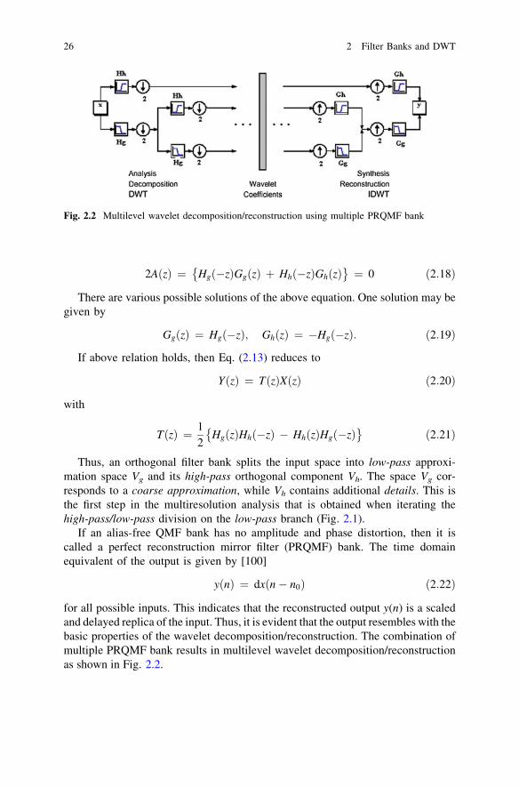
for all possible inputs. This indicates that the reconstructed output y(n) is a scaledand delayed replica of the input. Thus, it is evident that the output resembles with thebasic properties of the wavelet decomposition/reconstruction. The combination ofmultiple PRQMF bank results in multilevel wavelet decomposition/reconstructionas shown in Fig. 2.2.

Fig. 2.2 Multilevel wavelet decomposition/reconstruction using multiple PRQMF bank


2.2.2 Computational Complexity of Discrete WaveletTransform

Rioul et al. in their seminal paper [106] have studied the computational complexityof wavelet transforms in detail. In general, the computations are periodic in 2m foran m-level wavelet. Here, each filtered output is decimated by a factor of 2. Thisnecessitates computation of those signal samples that are not thrown away.Consider an input set of N = 2m samples. For the first level, each filter computesN/2 samples, so the total number of samples generated at the low-pass and high-pass filters of level-1 wavelet is N. Similarly, each filter in the second-levelwavelet computes N/4 samples, and the total number of samples computed at level2 is N/2. In an m-level wavelet, the total number of samples computed is

N þ N

2þ N

4þ � � � � � � þ 2 ¼ 2 N � 1ð Þ: ð2:23Þ

Since the wavelet computation is periodic with N samples, the number of samples

computed every sample period is 2 N � 1ð ÞN or 2 1 � 1

N

, which is upper bounded by 2[106]. This implies that the maximum number of filters needed for computation in aone-dimensional multilevel forward wavelet transform is two. In other words, onelow-pass and one high-pass filter will always be adequate for computation of one-dimensional DWT. The parallel filter bank structure discussed in next Section willlead to an efficient means for computation of wavelet transform.

2.3 Parallel Filter Bank Realization of Multilevel DiscreteWavelet Transform

As the computation of DWT involves filtering, an efficient filtering process isessential in DWT hardware implementation. A possible solution is based on Mallatalgorithm [87] requiring only two filters (one high- and one low-pass filter). In themultistage DWT, coefficients are calculated recursively, and in addition to thewavelet decomposition stage, extra space is required to store the intermediatecoefficients. Hence, the overall performance depends significantly on the precisionof the intermediate DWT coefficients [74] as discussed in detail in next chapter.An alternative method for fast and efficient implementation of DWT transform isbased on parallel filter implementation. In this, cascaded high-pass and low-passfilters at different resolution levels will be replaced by their equivalent filter [80],[107]. This necessitates number of filters to be of the order of decomposition level.The main advantage of the parallel filter algorithm is that it does not requirestoring intermediate coefficients [123]. Another advantage of this architecture isthat the word length can be arbitrary and is not restricted to be a multiple of 2m form-resolution-level wavelet decomposition.


As discussed, Fig. 2.2 is a multilevel representation of DWT. The DWTevaluation is based on binary tree structured QMF. The output from high-passfilter is termed as detailed wavelet coefficients and from low-pass filter is termed asapproximation coefficients. The approximation coefficients from previous level,after passing through another PRQMF filter bank, generate another set of detailedand approximation coefficients, and the decomposition process is continued untilone reaches desired level of decomposition. The limitation here is that if the DWTcoefficients of level L are of use, one has to first obtain the DWT coefficients atlevel L - 1, thus increasing computational burden. Souani et al. [123] presentedan efficient one-dimensional direct DWT computation algorithm. The algorithmenables computation of Lth-level DWT coefficients without prior knowledge of(L - 1)th-level DWT coefficients. The algorithm is simple and uses a modifiedfilter structure generated out of basic PRQMF filter bank. As discussed in nextchapters, the algorithm is suitable from finite precision and parallel implementa-tion viewpoint. Its implementation necessitates, finding equivalent parallel filtersgenerated out of PRQMF filter bank to compute the DWT coefficient at any levelfrom signal itself.

2.3.1 Iterated Filters and Regularity

The DWT filters roughly correspond to octave band filters. In many applications,low-frequency content of the signal is an important part. It is what gives the signalits identity. The high-frequency content, on the other hand, imparts flavor. Forexample, in the human voice, removing high-frequency components sounds dif-ferent, but contents can still be inferred. However, removal of the low-frequencycomponents sounds gibberish.

It is required to find the equivalent filter corresponding to the lower branch inFig. 2.2 that is the iterated low-pass filter. It can be easily checked that subsam-pling by two followed by filtering with G(z) is equivalent to filtering with G(z2)followed by the subsampling [80, 107]. Thus, the first two steps of low-passfiltering can be replaced with z-transform G(z). G(z2), followed by subsamplingby 4. In general, representing GJ(z) the equivalent filter to the Jth stages of low-pass filtering and subsampling by 2J [139]:

GJðzÞ ¼YJ� 1

l¼0

Gðz2lÞ ð2:24Þ

A necessary condition for the iterated functions to converge to a continuouslimit is that the filter G(z) should have sufficient number of zeros at z = -1, or halfsampling frequency, so as to attenuate repeat spectra [107]. Using this condition,the regular filters, which are both orthogonal and converge to continuous functionswith compact support, may be generated. The well-known Daubechies orthonor-mal filters [36] are deduced from maximally flat low-pass filters.


2.3.1.1 Generation of Parallel Filter Banks

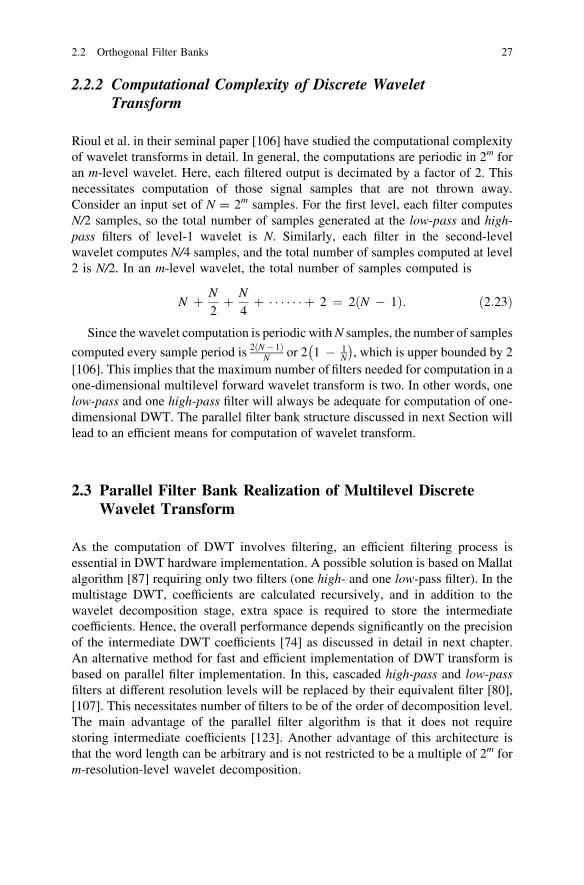
In present chapter for the sake of simplicity, the algorithm has been demonstratedonly for two levels and three levels of DWT decomposition. For L level, it can begeneralized there from. Consider the two-level DWT decomposition Mallat’salgorithm [87] and derived parallel filter equivalent as shown in Fig. 2.3.

The equivalent analysis filters for two-level DWT (Fig. 2.3) are expressed interms of PRQMF filter bank as follows:

B zð Þ ¼ H zð Þ ð2:25Þ

C zð Þ ¼ G zð ÞH z2

ð2:26Þ

D zð Þ ¼ G zð ÞG z2

ð2:27Þ

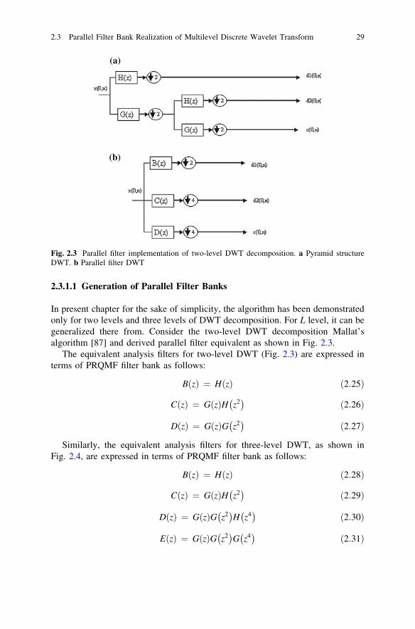
Similarly, the equivalent analysis filters for three-level DWT, as shown inFig. 2.4, are expressed in terms of PRQMF filter bank as follows:

B zð Þ ¼ H zð Þ ð2:28Þ

C zð Þ ¼ G zð ÞH z2

ð2:29Þ

D zð Þ ¼ G zð ÞG z2

H z4

ð2:30Þ

E zð Þ ¼ G zð ÞG z2

G z4

ð2:31Þ

(a)

(b)

Fig. 2.3 Parallel filter implementation of two-level DWT decomposition. a Pyramid structureDWT. b Parallel filter DWT

2.3 Parallel Filter Bank Realization of Multilevel Discrete Wavelet Transform 29

More generally for J-level decomposition, the equivalent filter to J stages oflow-pass filtering and subsampling by two (a total subsampling by 2J) is given by[107]

EJ zð Þ ¼YJ� 1

l¼0

GðZ2lÞ ð2:31Þ

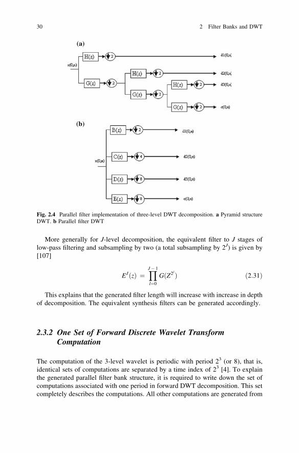
This explains that the generated filter length will increase with increase in depthof decomposition. The equivalent synthesis filters can be generated accordingly.

2.3.2 One Set of Forward Discrete Wavelet TransformComputation

The computation of the 3-level wavelet is periodic with period 23 (or 8), that is,identical sets of computations are separated by a time index of 23 [4]. To explainthe generated parallel filter bank structure, it is required to write down the set ofcomputations associated with one period in forward DWT decomposition. This setcompletely describes the computations. All other computations are generated from

(a)

(b)

Fig. 2.4 Parallel filter implementation of three-level DWT decomposition. a Pyramid structureDWT. b Parallel filter DWT


this set by shifting the time by multiples of the period. For simplicity, followingtransfer function representation of filters used in PRQMF filter bank with L–tapfilters is assumed as follows:

HðzÞ ¼XL� 1

n¼0

hðzÞz�n ð2:32Þ

GðzÞ ¼XL� 1

n¼0

gðzÞz�n ð2:33Þ

For simplicity, the filter tap is selected to L = 6.For details of multilevel DWT coefficient computation, readers are advised to

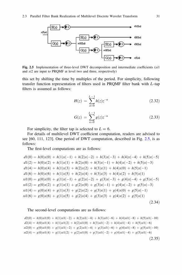
see [60, 111, 123]. One period of DWT computation, described in Fig. 2.5, is asfollows:

The first-level computations are as follows:

d1ð0Þ ¼ hð0Þxð0Þ þ hð1Þxð�1Þ þ hð2Þxð�2Þ þ hð3Þxð�3Þ þ hð4Þxð�4Þ þ hð5Þxð�5Þd1ð2Þ ¼ hð0Þxð2Þ þ hð1Þxð1Þ þ hð2Þxð0Þ þ hð3Þxð�1Þ þ hð4Þxð�2Þ þ hð5Þxð�3Þd1ð4Þ ¼ hð0Þxð4Þ þ hð1Þxð3Þ þ hð2Þxð2Þ þ hð3Þxð1Þ þ hð4Þxð0Þ þ hð5Þxð�1Þd1ð6Þ ¼ hð0Þxð6Þ þ hð1Þxð5Þ þ hð2Þxð4Þ þ hð3Þxð3Þ þ hð4Þxð2Þ þ hð5Þxð1Þxi1ð0Þ ¼ gð0Þxð0Þ þ gð1Þxð�1Þ þ gð2Þxð�2Þ þ gð3Þxð�3Þ þ gð4Þxð�4Þ þ gð5Þxð�5Þxi1ð2Þ ¼ gð0Þxð2Þ þ gð1Þxð1Þ þ gð2Þxð0Þ þ gð3Þxð�1Þ þ gð4Þxð�2Þ þ gð5Þxð�3Þxi1ð4Þ ¼ gð0Þxð4Þ þ gð1Þxð3Þ þ gð2Þxð2Þ þ gð3Þxð1Þ þ gð4Þxð0Þ þ gð5Þxð�1Þxi1ð6Þ ¼ gð0Þxð6Þ þ gð1Þxð5Þ þ gð2Þxð4Þ þ gð3Þxð3Þ þ gð4Þxð2Þ þ gð5Þxð1Þ

ð2:34Þ

The second-level computations are as follows:

d2ð0Þ ¼ hð0Þxi1ð0Þ þ hð1Þxi1ð�2Þ þ hð2Þxi1ð�4Þ þ hð3Þxi1ð�6Þ þ hð4Þxi1ð�8Þ þ hð5Þxi1ð�10Þd2ð4Þ ¼ hð0Þxi1ð4Þ þ hð1Þxi1ð2Þ þ hð2Þxi1ð0Þ þ hð3Þxi1ð�2Þ þ hð4Þxi1ð�4Þ þ hð5Þxi1ð�6Þxi2ð0Þ ¼ gð0Þxi1ð0Þ þ gð1Þxi1ð�2Þ þ gð2Þxi1ð�4Þ þ gð3Þxi1ð�6Þ þ gð4Þxi1ð�8Þ þ gð5Þxi1ð�10Þxi2ð4Þ ¼ gð0Þxi1ð4Þ þ gð1Þxi1ð2Þ þ gð2Þxi1ð0Þ þ gð3Þxi1ð�2Þ þ gð4Þxi1ð�4Þ þ gð5Þxi1ð�6Þ

ð2:35Þ

Fig. 2.5 Implementation of three-level DWT decomposition and intermediate coefficients (xi1and xi2 are input to PRQMF at level two and three, respectively)


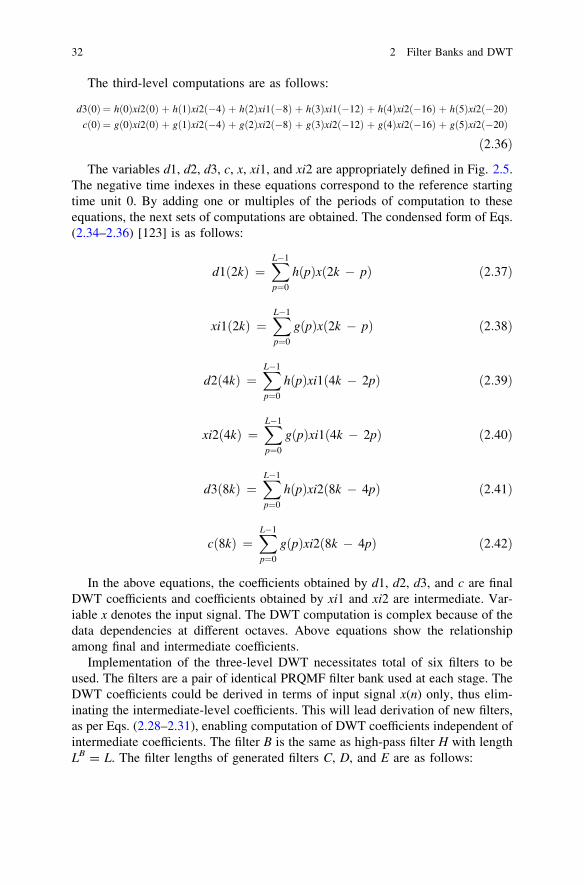
The third-level computations are as follows:

d3ð0Þ ¼ hð0Þxi2ð0Þ þ hð1Þxi2ð�4Þ þ hð2Þxi1ð�8Þ þ hð3Þxi1ð�12Þ þ hð4Þxi2ð�16Þ þ hð5Þxi2ð�20Þcð0Þ ¼ gð0Þxi2ð0Þ þ gð1Þxi2ð�4Þ þ gð2Þxi2ð�8Þ þ gð3Þxi2ð�12Þ þ gð4Þxi2ð�16Þ þ gð5Þxi2ð�20Þ

ð2:36Þ

The variables d1, d2, d3, c, x, xi1, and xi2 are appropriately defined in Fig. 2.5.The negative time indexes in these equations correspond to the reference startingtime unit 0. By adding one or multiples of the periods of computation to theseequations, the next sets of computations are obtained. The condensed form of Eqs.(2.34–2.36) [123] is as follows:

d1ð2kÞ ¼XL�1

p¼0

hðpÞxð2k � pÞ ð2:37Þ

xi1ð2kÞ ¼XL�1

p¼0

gðpÞxð2k � pÞ ð2:38Þ

d2ð4kÞ ¼XL�1

p¼0

hðpÞxi1ð4k � 2pÞ ð2:39Þ

xi2ð4kÞ ¼XL�1

p¼0

gðpÞxi1ð4k � 2pÞ ð2:40Þ

d3ð8kÞ ¼XL�1

p¼0

hðpÞxi2ð8k � 4pÞ ð2:41Þ

cð8kÞ ¼XL�1

p¼0

gðpÞxi2ð8k � 4pÞ ð2:42Þ

In the above equations, the coefficients obtained by d1, d2, d3, and c are finalDWT coefficients and coefficients obtained by xi1 and xi2 are intermediate. Var-iable x denotes the input signal. The DWT computation is complex because of thedata dependencies at different octaves. Above equations show the relationshipamong final and intermediate coefficients.

Implementation of the three-level DWT necessitates total of six filters to beused. The filters are a pair of identical PRQMF filter bank used at each stage. TheDWT coefficients could be derived in terms of input signal x(n) only, thus elim-inating the intermediate-level coefficients. This will lead derivation of new filters,as per Eqs. (2.28–2.31), enabling computation of DWT coefficients independent ofintermediate coefficients. The filter B is the same as high-pass filter H with lengthLB = L. The filter lengths of generated filters C, D, and E are as follows:


LC ¼ 3L � 2

LD ¼ 7L � 6

LE ¼ 7L � 6

ð2:43Þ

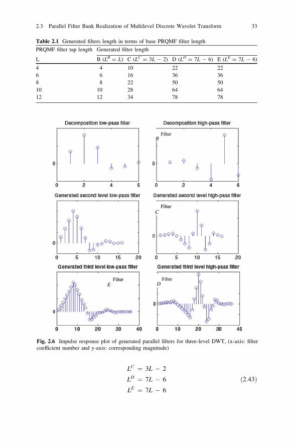
Table 2.1 Generated filters length in terms of base PRQMF filter length

PRQMF filter tap length Generated filter length

L B (LB = L) C (LC = 3L - 2) D (LD = 7L - 6) E (LE = 7L - 6)

4 4 10 22 226 6 16 36 368 8 22 50 5010 10 28 64 6412 12 34 78 78

Fig. 2.6 Impulse response plot of generated parallel filters for three-level DWT, (x-axis: filtercoefficient number and y-axis: corresponding magnitude)


The generated parallel filters lengths for varied PRQMF filter lengths are givenin Table 2.1. It is evident that the filter B operates every two samples (down-sampling by 2). Filter C operates every four samples; filters D and E operate everyeight samples. For an even order of the input data, filters B, C, D, and E willoperate depending on their decimation rate.

2.4 Frequency Response of Generated Parallel Filter Bank

To validate the parallel filter DWT structure, frequency response plots are gen-erated. The frequency response plots corresponding to three-level DWT decom-position are shown. The selected PRQMF filter bank is a Daubechies filter [37]with six taps, and Symlet filter [14] with eight taps. The experimentation has beencarried out on a Pentium III, 733 MHz system using Matlab [93].

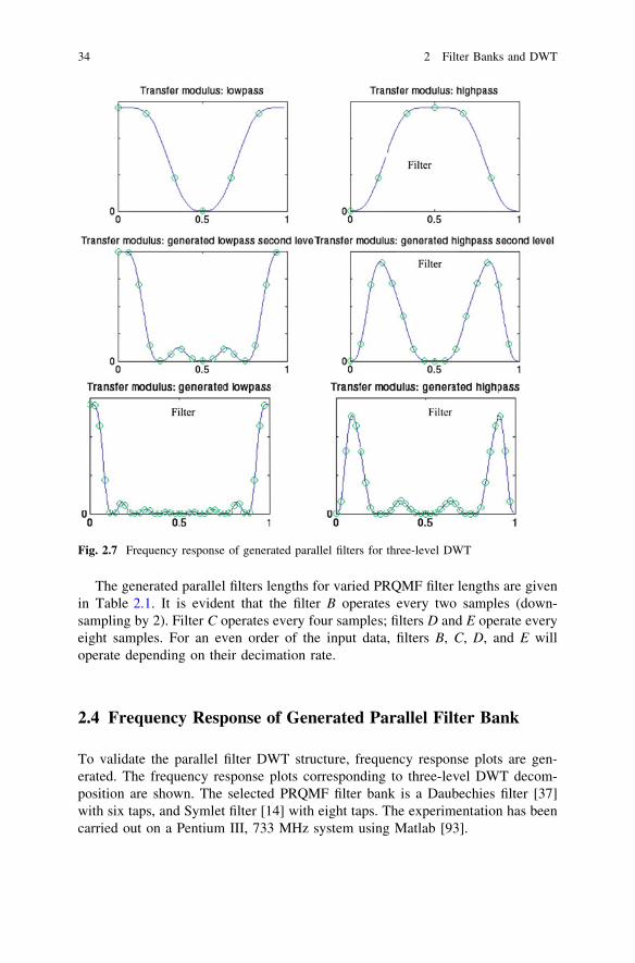
Fig. 2.7 Frequency response of generated parallel filters for three-level DWT


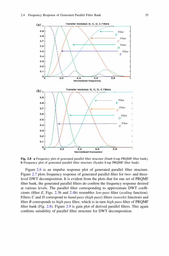
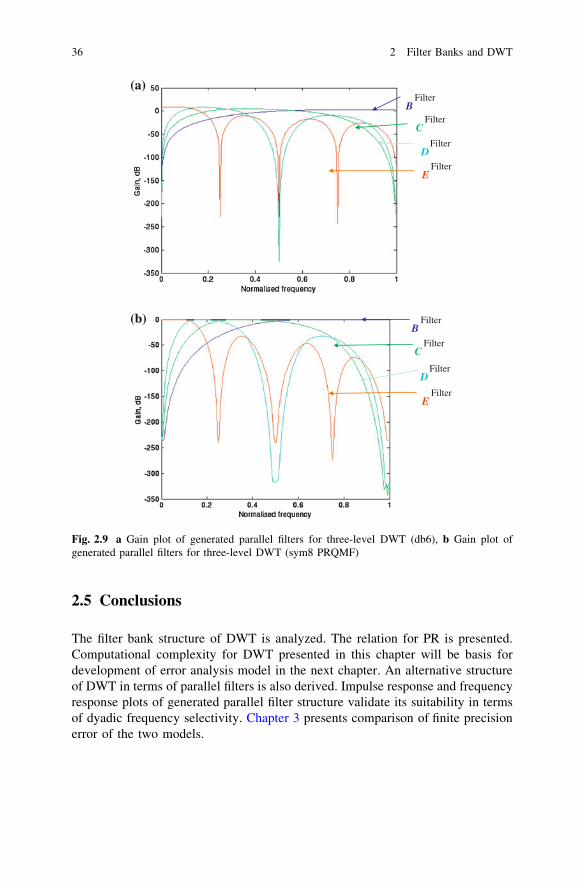
Figure 2.6 is an impulse response plot of generated parallel filter structure.Figure 2.7 plots frequency response of generated parallel filter for two- and three-level DWT decomposition. It is evident from the plots that for one set of PRQMFfilter bank, the generated parallel filters do confirm the frequency response desiredat various levels. The parallel filter corresponding to approximate DWT coeffi-cients (filter E, Figs. 2.3b and 2.4b) resembles low-pass filter (scaling function).Filters C and D correspond to band-pass (high-pass) filters (wavelet function) andfilter B corresponds to high-pass filter, which is in turn high-pass filter of PRQMFfilter bank (Fig. 2.8). Figure 2.9 is gain plot of derived parallel filters. This againconfirms suitability of parallel filter structure for DWT decomposition.

Filter B

Filter C

Filter D

Filter E

Filter B

Filter C

Filter D

Filter E

(a)

(b)

Fig. 2.8 a Frequency plot of generated parallel filter structure (Daub 6-tap PRQMF filter bank),b Frequency plot of generated parallel filter structure (Symlet 8-tap PRQMF filter bank)

2.4 Frequency Response of Generated Parallel Filter Bank 35

2.5 Conclusions

The filter bank structure of DWT is analyzed. The relation for PR is presented.Computational complexity for DWT presented in this chapter will be basis fordevelopment of error analysis model in the next chapter. An alternative structureof DWT in terms of parallel filters is also derived. Impulse response and frequencyresponse plots of generated parallel filter structure validate its suitability in termsof dyadic frequency selectivity. Chapter 3 presents comparison of finite precisionerror of the two models.

Filter B

Filter C

Filter D

Filter E

Filter B

Filter C

Filter D

Filter E

(a)

(b)

Fig. 2.9 a Gain plot of generated parallel filters for three-level DWT (db6), b Gain plot ofgenerated parallel filters for three-level DWT (sym8 PRQMF)


http://dx.doi.org/10.1007/978-1-4471-4941-5_3

Documents

Chapter 2 Filter Banks and DWT