Embed Size (px)
Citation preview
Filter Banks for Next Generation Multicarrier Wireless Communications
Guest Editors: Markku Renfors, Pierre Siohan, Behrouz Farhang-Boroujeny, and Faouzi Bader
EURASIP Journal on Advances in Signal Processing
Filter Banks for Next Generation MulticarrierWireless Communications
EURASIP Journal on Advances in Signal Processing
Filter Banks for Next Generation MulticarrierWireless Communications
Guest Editors: Markku Renfors, Pierre Siohan,Behrouz Farhang-Boroujeny, and Faouzi Bader

Copyright © 2010 Hindawi Publishing Corporation. All rights reserved.
This is a special issue published in volume 2010 of “EURASIP Journal on Advances in Signal Processing.” All articles are open accessarticles distributed under the Creative Commons Attribution License, which permits unrestricted use, distribution, and reproduction inany medium, provided the original work is properly cited.
Editor-in-ChiefPhillip Regalia, Institut National des Telecommunications, France
Associate Editors
Adel M. Alimi, TunisiaKenneth Barner, USAYasar Becerikli, TurkeyKostas Berberidis, GreeceJose Carlos Bermudez, BrazilEnrico Capobianco, ItalyA. Enis Cetin, TurkeyJonathon Chambers, UKMei-Juan Chen, TaiwanLiang-Gee Chen, TaiwanHuaiyu Dai, USASatya Dharanipragada, USAKutluyil Dogancay, AustraliaFlorent Dupont, FranceFrank Ehlers, ItalySharon Gannot, IsraelM. Greco, ItalyIrene Y. H. Gu, SwedenFredrik Gustafsson, SwedenUlrich Heute, GermanySangjin Hong, USAJiri Jan, Czech RepublicMagnus Jansson, SwedenSudharman K. Jayaweera, USA
Soren Holdt Jensen, DenmarkMark Kahrs, USAMoon Gi Kang, South KoreaWalter Kellermann, GermanyLisimachos P. Kondi, GreeceAlex Chichung Kot, SingaporeC.-C. Jay Kuo, USAErcan E. Kuruoglu, ItalyTan Lee, ChinaGeert Leus, The NetherlandsT.-H. Li, USAHusheng Li, USAMark Liao, TaiwanY.-P. Lin, TaiwanShoji Makino, JapanStephen Marshall, UKC. Mecklenbrauker, AustriaGloria Menegaz, ItalyRicardo Merched, BrazilMarc Moonen, BelgiumVitor Heloiz Nascimento, BrazilChristophoros Nikou, GreeceSven Nordholm, AustraliaPatrick Oonincx, The Netherlands
Douglas O’Shaughnessy, CanadaBjorn Ottersten, SwedenJacques Palicot, FranceAna Perez-Neira, SpainWilfried R. Philips, BelgiumAggelos Pikrakis, GreeceIoannis Psaromiligkos, CanadaAthanasios Rontogiannis, GreeceGregor Rozinaj, SlovakiaMarkus Rupp, AustriaWilliam Allan Sandham, UKBulent Sankur, TurkeyLing Shao, UKDirk Slock, FranceY.-P. Tan, SingaporeJoao Manuel R. S. Tavares, PortugalGeorge S. Tombras, GreeceDimitrios Tzovaras, GreeceBernhard Wess, AustriaJar-Ferr Yang, TaiwanAzzedine Zerguine, Saudi ArabiaAbdelhak M. Zoubir, Germany
Contents
Filter Banks for Next Generation Multicarrier Wireless Communications, Markku Renfors, Pierre Siohan,Behrouz Farhang-Boroujeny, and Faouzi BaderVolume 2010, Article ID 314193, 2 pages
Cosine Modulated and Offset QAM Filter Bank Multicarrier Techniques: A Continuous-Time Prospect,Behrouz Farhang-Boroujeny and Chung Him (George) YuenVolume 2010, Article ID 165654, 16 pages
Design of Orthogonal Filtered Multitone Modulation Systems and Comparison among EfficientRealizations, Nicola Moret and Andrea M. TonelloVolume 2010, Article ID 141865, 18 pages
Optimized Paraunitary Filter Banks for Time-Frequency Channel Diagonalization, Ziyang Ju,Thomas Hunziker, and Dirk DahlhausVolume 2010, Article ID 172751, 12 pages
Spectral Efficiency Comparison of OFDM/FBMC for Uplink Cognitive Radio Networks, H. Zhang,D. Le Ruyet, D. Roviras, Y. Medjahdi, and H. SunVolume 2010, Article ID 621808, 14 pages
Computationally Efficient Power Allocation Algorithm in Multicarrier-Based Cognitive Radio Networks:OFDM and FBMC Systems, Musbah Shaat and Faouzi BaderVolume 2010, Article ID 528378, 13 pages
Packet Format Design and Decision Directed Tracking Methods for Filter Bank Multicarrier Systems,Peiman Amini and Behrouz Farhang-BoroujenyVolume 2010, Article ID 307983, 13 pages
Joint Symbol Timing and CFO Estimation for OFDM/OQAM Systems in Multipath Channels,Tilde Fusco, Angelo Petrella, and Mario TandaVolume 2010, Article ID 897607, 11 pages
Pilot-Based Synchronization and Equalization in Filter Bank Multicarrier Communications,Tobias Hidalgo Stitz, Tero Ihalainen, Ari Viholainen, and Markku RenforsVolume 2010, Article ID 741429, 18 pages
Decoding Schemes for FBMC with Single-Delay STTC, Chrislin Lele and Didier Le RuyetVolume 2010, Article ID 689824, 11 pages
The Alamouti Scheme with CDMA-OFDM/OQAM, Chrislin Lele, Pierre Siohan, and Rodolphe LegouableVolume 2010, Article ID 703513, 13 pages
Hindawi Publishing CorporationEURASIP Journal on Advances in Signal ProcessingVolume 2010, Article ID 314193, 2 pagesdoi:10.1155/2010/314193
Editorial
Filter Banks for Next Generation MulticarrierWireless Communications
Markku Renfors (EURASIP Member),1 Pierre Siohan,2
Behrouz Farhang-Boroujeny,3 and Faouzi Bader4
1 Department of Communications Engineering, Tampere University of Technology, P.O. Box 553, 33101 Tampere, Finland2 Orange Labs, France Telecom, 4 Rue du Clos Courtel, B.P. 91226, 35512 Cesson Sevigne Cedex, France3 Department of Electrical and Computer Engineering, University of Utah, Salt Lake City, UT 84112-9206, USA4 Centre Tecnologic de Telecommunication de Catalunya (CTTC), Parc Mediterrani de la Tecnologia,Avinguda del Canal Olimpic, Casstelldefels, 08860 Barcelona, Spain
Correspondence should be addressed to Markku Renfors, [email protected]
Received 3 May 2010; Accepted 3 May 2010
Copyright © 2010 Markku Renfors et al. This is an open access article distributed under the Creative Commons AttributionLicense, which permits unrestricted use, distribution, and reproduction in any medium, provided the original work is properlycited.
The theoretical capacity limits in communications can beapproached by multicarrier techniques. With radio channels,multicarrier techniques can be combined with multiantennatransmitters and receivers to provide efficiency. Existing orplanned transmission systems rely on the OFDM techniqueto reach these goals and a considerable amount of researchhas been devoted to these techniques during the last 20years. However OFDM has a number of drawbacks, suchas the use of the cyclic prefix to cope with the channelimpulse response which results in a loss of capacity and therequirement of block processing to maintain orthogonalityamong all the subcarriers. Furthermore, the leakage amongfrequency subbands has a serious impact on the performanceof FFT-based spectrum sensing and OFDM-based cognitiveradio in general.
On the other hand, digital filter banks find variousgood applications in communications signal processing. Ingeneral, they can be used to obtain very sharp frequencyselectivity to isolate different communications frequencychannels from each other and from interfering spectralcomponents. This can be done in a very flexible anddynamic manner. Thus filter banks constitute a very powerfulgeneric tool for software-defined radios and spectrally agilecommunication systems.
So far, some attempts have been made to introduce filterbank multicarrier (FBMC) in the radio communicationsarena, through proprietary schemes, in particular the IOTA
(Isotropic Orthogonal Transform Algorithm). However, thefull exploitation and optimization of FBMC techniques in thecontext of radio evolution, such as dynamic access, as wellas their combination with MIMO techniques, have not beenconsidered sufficiently.
This special issue aims to report advances in thesecommunication aspects of FBMC, helping to make full useof FBMC as a new physical layer for future radio communi-cation systems. We received 18 submission altogether, out ofwhich ten were accepted through a peer review process.
The first paper, “Cosine modulated and offset QAM filterbank multicarrier techniques: a continuous-time prospect”authored by B. Farhang-Boroujeny and C. H. (George)Yuen, presents a tutorial review relating the classical workson FBMC systems, developed prior of the era of OFDM,to the main filter bank design approaches used today forFBMC systems. The paper also reviews the recent noveldevelopments in the design of FBMC systems that are tunedto cope with fast fading wireless channels.
N. Moret and A. M. Tonello address the efficientrealization of a filtered multitone (FMT) modulation systemin the second paper entitled “Design of orthogonal filteredmultitone modulation systems and comparison among efficientrealizations”. The paper analyzes three different realizationstructures, presenting also numerical comparisons, andcompares the best FMT approach with a cyclically prefixedOFDM system in the IEEE 802.11 wireless LAN channel.
2 EURASIP Journal on Advances in Signal Processing
The third paper, “Optimized paraunitary filter banks fortime-frequency channel diagonalization” by Z. Ju et al. devel-ops a method to diagonalize a doubly dispersive channel inthe time-frequency domain using a filter bank approach. Therelated paraunitary filter bank design problem is formulatedas a convex optimization problem, and the performance ofthe resulting window is investigated under different channelconditions.
The fourth paper, “Spectral efficiency comparison ofOFDM/FBMC for uplink cognitive radio networks” by H.Zhang et al. studies channel capacity of cognitive radio(CR) networks using CP-OFDM and FBMC waveforms,taking into consideration the effects of resource allocationalgorithms, intercell interference due to timing offsets, andRayleigh fading. Final results show that FBMC can achievehigher channel capacity than OFDM because of the lowspectral leakage of its prototype filter.
M. Shaat and F. Bader address the problem of resourceallocation in multicarrier-based CR networks in the fifthpaper entitled “Computationally efficient power allocationalgorithm in multicarrier-based cognitive radio networks:OFDM and FBMC systems”. The objective is to maximize thedownlink capacity of the network under constraints on bothtotal power and interference introduced to the primary users.The performance of the proposed low-complexity algorithmis investigated for OFDM- and FBMC-based CR systems.
In the sixth paper, “Packet format design and decisiondirected tracking methods for filter bank multicarrier systems”,P. Amini and B. Farhang-Boroujeny develop a packet formatfor FBMC systems together with algorithms for carrierfrequency and timing recovery. Also methods for channelestimation as well as carrier and timing tracking loops areproposed.
In the seventh paper, entitled “Joint symbol timing andCFO estimation for OFDM/OQAM systems in multipathchannels”, T. Fusco et al. develop different maximum-likelihood based approaches for estimating carrier-frequencyoffsets and symbol timing offsets using short preambles inthe FBMC transmission bursts. Good performance for a low-complexity approximate ML estimator is demonstrated.
The eighth paper, “Pilot-based synchronization and equal-ization in filter bank multicarrier communications” authoredby T. H. Stitz et al., presents a detailed analysis of synchro-nization and channel estimation methods for FBMC basedon scattered pilots. The special problems related to usingscattered pilot-based schemes in FBMC are highlighted.The channel parameter estimation and compensation aresuccessfully performed totally in the frequency domain, ina subchannel-wise fashion, which is appealing in spectrallyagile and cognitive radio scenarios.
The ninth paper is entitled “Decoding schemes for FBMCwith single-delay STTC” and authored by C. Lele and D.Le Ruyet. The paper develops space-time trellis codingschemes for FBMC, addressing the challenge that the OQAMsignal model of FBMC makes the decoding process morechallenging compared to the CP-OFDM case. The developediterative decoding scheme for FBMC is shown to slightlyoutperform CP-OFDM.
The tenth paper, “The Alamouti scheme with CDMA-OFDM/OQAM” by C. Lele et al. introduces first the fact thatthe well-known Alamouti decoding scheme cannot be simplycombined with the OQAM subcarrier modulation scheme ofFBMC. The paper then develops Alamouti coding schemesby combining CDMA component with OFDM/OQAM.
We would like to thank all authors for their contributionsto our special issue, the reviewers for their help in selectingpapers, and the Editor-in-Chief Phillip Regalia and theEditorial Office of the Journal for their support.
Markku RenforsPierre Siohan
Behrouz Farhang-BoroujenyFaouzi Bader
Hindawi Publishing CorporationEURASIP Journal on Advances in Signal ProcessingVolume 2010, Article ID 165654, 16 pagesdoi:10.1155/2010/165654
Research Article
Cosine Modulated and Offset QAM Filter BankMulticarrier Techniques: A Continuous-Time Prospect
Behrouz Farhang-Boroujeny and Chung Him (George) Yuen
ECE Department, University of Utah, UT 84112, USA
Correspondence should be addressed to Behrouz Farhang-Boroujeny, [email protected]
Received 11 May 2009; Revised 23 September 2009; Accepted 14 December 2009
Academic Editor: Pierre Siohan
Copyright © 2010 B. Farhang-Boroujeny and C. H. (George) Yuen. This is an open access article distributed under the CreativeCommons Attribution License, which permits unrestricted use, distribution, and reproduction in any medium, provided theoriginal work is properly cited.
Prior to the discovery of the celebrated orthogonal frequency division multiplexing (OFDM), multicarrier techniques that useanalog filter banks were introduced in the 1960s. Moreover, advancements in the design of perfect reconstruction filter banks haveled to a number developments in the design of prototype digital filters and polyphase structures for efficient implementations ofthe filter bank multicarrier (FBMC) systems. The main thrust of this paper is to present a tutorial review of the classical works onFBMC systems and show that some of the more recent developments are, in fact, reinventions of multicarrier techniques that havebeen developed prior of the era of OFDM. We also review the recent novel developments in the design of FBMC systems that aretuned to cope with fast fading wireless channels.
1. Introduction
Orthogonal frequency division multiplexing (OFDM) is themost dominant technology that has been researched andhas been deployed for broadband wireless communications.OFDM is attractive because of a number of advantagesthat it offers. First, orthogonality of subcarrier channelsallows trivial equalization; one scalar gain per subcarrier.Second, closely spaced orthogonal subcarriers partition theavailable bandwidth into a collection of narrow subbands.Adaptive modulation schemes are then applied to sub-bandsto maximize bandwidth efficiency/transmission rate. Third,the very special structure of OFDM symbols simplifies thetasks of carrier and symbol synchronizations. These pointsare well understood and documented in the literature [1, 2].
More recent works propose extending the use of OFDMto multiple access applications. Multiple access OFDM, ororthogonal frequency division multiple access (OFDMA),has recently been proposed in a number of standards andproprietary waveforms (e.g., [3]). Some particular forms ofOFDMA have also been proposed for cognitive radio systems[4]. In OFDMA, a subset of the subcarriers is allocated toeach user node in a network. These users signals must be
synchronized at the receiver input to prevent intercarrierinterference. OFDMA works well in the network downlinkof a base station, since all of the subcarriers are transmittedfrom the same base station and, thus, can easily be syn-chronized. However, synchronization is not trivial in thenetwork uplink where a number of nodes are transmittingseparately. For OFDMA to work well in this scenario, thesignals from various nodes must be synchronized at the basestation, that is, they should be received as a set of orthogonalsignals. Since, in practice, perfect synchronization may notbe possible, additional signal processing steps have to betaken to minimize interference among signals from differentnodes. Such steps add significant complexity to an OFDMAreceiver; see [5] and the references therein. The problemis worse in a cognitive radio setting where both primary(non-cognitive nodes) and secondary users (cognitive nodes)transmit independently and may be based on differentstandards. Therefore, the existing OFDMA may not be ableto satisfactorily address the needs of efficient use of spectrain the next generation of communication networks.
Clearly, the above problem could be greatly alleviatedif the filters that synthesize the subcarrier signals hadsmall side-lobes. An interesting, but apparently not widely
2 EURASIP Journal on Advances in Signal Processing
understood, fact is that the first multicarrier techniqueswhich were developed before the invention of OFDM usedfilter banks for synthesis and analysis of multicarrier signals.Such filter banks can be designed with small side-lobes,thus, are ideal choice in multiple access and cognitive radioapplications [6]. The first proposal came from Chang [7],who presented the conditions required for signaling a parallelset of pulse amplitude modulated (PAM) symbol sequencesthrough a bank of overlapping filters within a minimumbandwidth. To transmit PAM symbols in a bandwidthefficient manner, Chang’s signaling is based on staggering anumber of overlapping vestigial side-band (VSB) modulatedsignal sequences. Saltzberg [8], extended the idea and showedhow the Chang’s method could be modified for transmissionof quadrature amplitude modulated (QAM) symbols, ina double side-band modulated format. Efficient digitalimplementation of Saltzberg’s multicarrier system throughpolyphase structures first introduced by Bellanger et al.[9, 10], was studied by Hirosaki [11, 12], and was furtherdeveloped by others [13–21]. Both Chang’s and Saltzberg’smethods belong to a class of multicarrier techniques that maybe referred to as filter bank multicarrier (FBMC) systems.
The pioneering work of Chang [7], on the other hand,has received less attention within the signal processing com-munity. Those who have cited [7], have only acknowledgedits existence without presenting much details, for example[11, 16, 19, 22]. For instance, Hirosaki who has extensivelystudied and developed digital structures for implementationof Saltzberg’s method, [11, 16], has made a brief reference toChang’s method and noted that since it uses VSB modulationand thus its implementation require a Hilbert transforma-tion, it is more complex than that of Saltzberg’s method.He thus proceeds with a detail discussion and developmentof multirate structures for the Saltzberg’s method only. Onthe other hand, a vast literature in digital signal processinghas studied a class of multicarrier systems that has beenreferred to as discrete wavelet multitone (DWMT). Theinitial works on DWMT are [23–25]. In the period of 1995to 2003 a fair number of contributions from various authorsappeared in the literature, for example [26–30]. Reference[30], in particular, did a thorough study of DWMT andnoted that this method operates based on cosine modulatedfilter banks which were extensively developed in the 1980’sin the context of compression techniques [31]. The fact thatDWMT uses cosine modulated filter banks has also beenacknowledged by other authors, for example [28]. Reference[30] also greatly simplified the equalizer structure that wasoriginally proposed in [23–25] and widely adopted by others.Moreover, [30] noted that a DWMT signal is synthesized byaggregating a set of VSB modulated PAM signal sequences.However, most of the works on DWMT (including [30]) havemade no direct reference to Chang’s method. In other words,the Chang’s multicarrier method was re-invented, with astrong multirate signal processing flavor, in the 1990’s. Partof our attempt in this paper is to show this very importantrelationship between what has been done over 40 yearsago, and the independent developments on DWMT/cosinemodulated multicarrier techniques that have been developedin more recent years. We also hope that the tutorial treatment
of the Chang’s method in this paper will facilitate a morein-depth understanding of the DWMT/cosine modulatedmulticarrier literature. Another important point to note isthat although DWMT was originally developed with DSLapplications in mind, it was never adopted in any of DSLstandards. However, DWMT has recently found its way topower line communications (PLC) that share a very similarenvironment to that of DSL [32].
It is also interesting to note that the researchers whostudied filter banks developed a class of filter banks whichwere called modified DFT (MDFT) filter bank [33]. Carefulstudy of MDFT reveals that this, although done indepen-dently, is in effect a reformulation of Saltzberg’s filter bankin discrete-time and with emphasis on compression/coding.The literature on MDFT begins with the pioneering worksof Fliege [34], and later has been extended by others, forexample [35–38].
As a final note in this introductory section, we wishto bring the attention of reader to various terminologiesthat have appeared in the literature related to Chang’s andSaltzberg’s MCFB methods and many further extensionsthat have been made by others. In the pioneering works ofChang [7] and Saltzberg [8] no specific name has been givento the multicarrier modulation types that they introduce,except that Chang notes PAM symbols are transmittedvia its signaling method and Saltzberg notes that howQAM symbols can be transmitted with the same bandwidthefficiency. Even the fact that Chang’s subcarrier modulationis VSB has not been explicitly noted in his paper [7].Apparently, the name staggered QAM was used for thetype of modulation suggested in [8], for the first time, in[39]. Later, Hirosaki [12] used the terminology orthogonallymultiplexed QAM (OQAM). OQAM was later referred to asOFDM-OQAM by many authors, for example [13–15, 17–21], with the acronym OQAM standing for offset QAM,reflecting the fact that the in-phase and quadrature of eachQAM symbol are time offset with respect to each other.A few others have named it pulse-shaped OFDM [40–47]. These use of different terminologies in parallel withthe independent introduction of MDFT, which is based onthe same fundamental principles as OQAM, has made theliterature on FBMC techniques somewhat blurred [48], andthus confusing to any novice who wishes to begin a researchin this area.
The same is true for Chang’s method and the inde-pendent, but related, works that have been published later.Among these [25], that received a significant level ofattention (see [30] and the references therein), independently(but, effectively) presented Chang’s modulation schemeunder the name discrete wavelet multitone (DWMT). Thename DWMT is somewhat confusing here as the proposedmethod in fact uses cosine modulated filter banks for whichthe use of the terminology wavelet is a misnomer. Cosinemodulated filter banks belong to the class of uniformfilter banks, meaning that all subbands have the samewidth. Wavelets, on the other hand, are referred to filterbanks whose subband widths increase exponentially withthe respective carrier/center frequencies. The adjective dyadicis often used to address this property of wavelets. It is
EURASIP Journal on Advances in Signal Processing 3
also interesting to note that there exists another class ofmulticarrier techniques that are based on true wavelets (i.e.,wavelets with dyadic bandwidths), for example, see [49].Moreover, it is worth noting that the IEEE P1901 workinggroup who has adopted a DWMT type modulation forpart of PLC standard, has called it wavelet-OFDM. Onthe other hand, some authors have preferred the namecosine modulated filter bank OFDM (CMFB-OFDM). In[50], where a more thorough study of DWMT/CMFB-OFDM to VDSL has been presented, the shorter namecosine-modulated multitone (CMT) has been proposed,following the terminology filtered multitone (FMT) [51–53], another FBMC candidate that was proposed (but wasnever adopted) in VDSL standard. In this paper, we useCMT when reference is made to the Chang’s method (andits extensions). We also introduce and use the terminologystaggered-modulated multitone (SMT) for the Saltzberg’smethod (and its extensions).
In this paper, we first present a novel tutorial reviewof Chang’s and Saltzberg’s FBMC methods with the goal ofmaking these classical works more accessible to the signalprocessing community. These are presented in Sections 2 and3, respectively. Similarities and differences of CMT and SMTare discussed in Section 4. In Section 5 further developmentthat has been made on extensions on Chang’s and Saltzberg’smethods are discussed. The emphasis in this section is onthe design of prototype filters for CMT and SMT. A briefreview of equalization of CMT and SMT systems is presentedin Section 6. The concluding remarks are made in Section 7.
Even though, any modern implementation of a CMTor SMT system will be in discrete-time, the derivationsin this paper are in terms of continuous-time signals andsystems. The choice of the continuous-time formulation heresimplifies the derivations and will also provide more insightto the fundamental properties of both CMT and SMT as wellas their similarities and differences. We believe our approachalso provides a meaningful intuitive understanding of theextension of CMT and SMT that are discussed in Section 5.
2. Cosine Modulated Multitone (CMT)
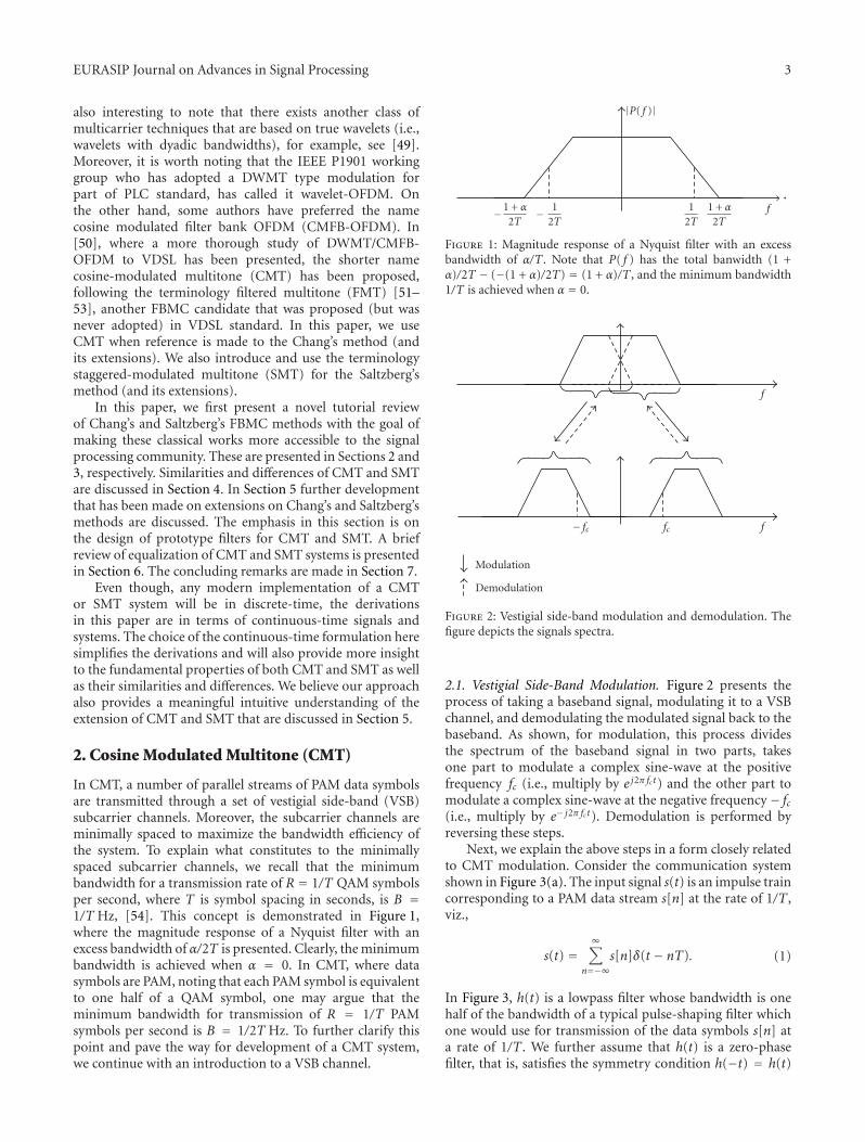
In CMT, a number of parallel streams of PAM data symbolsare transmitted through a set of vestigial side-band (VSB)subcarrier channels. Moreover, the subcarrier channels areminimally spaced to maximize the bandwidth efficiency ofthe system. To explain what constitutes to the minimallyspaced subcarrier channels, we recall that the minimumbandwidth for a transmission rate of R = 1/T QAM symbolsper second, where T is symbol spacing in seconds, is B =1/T Hz, [54]. This concept is demonstrated in Figure 1,where the magnitude response of a Nyquist filter with anexcess bandwidth of α/2T is presented. Clearly, the minimumbandwidth is achieved when α = 0. In CMT, where datasymbols are PAM, noting that each PAM symbol is equivalentto one half of a QAM symbol, one may argue that theminimum bandwidth for transmission of R = 1/T PAMsymbols per second is B = 1/2T Hz. To further clarify thispoint and pave the way for development of a CMT system,we continue with an introduction to a VSB channel.
|P( f )|
− 1 + α
2T− 1
2T1
2T1 + α
2Tf
Figure 1: Magnitude response of a Nyquist filter with an excessbandwidth of α/T . Note that P( f ) has the total banwidth (1 +α)/2T − (−(1 + α)/2T) = (1 + α)/T , and the minimum bandwidth1/T is achieved when α = 0.
Modulation
Demodulation
f
− fc fc f
Figure 2: Vestigial side-band modulation and demodulation. Thefigure depicts the signals spectra.
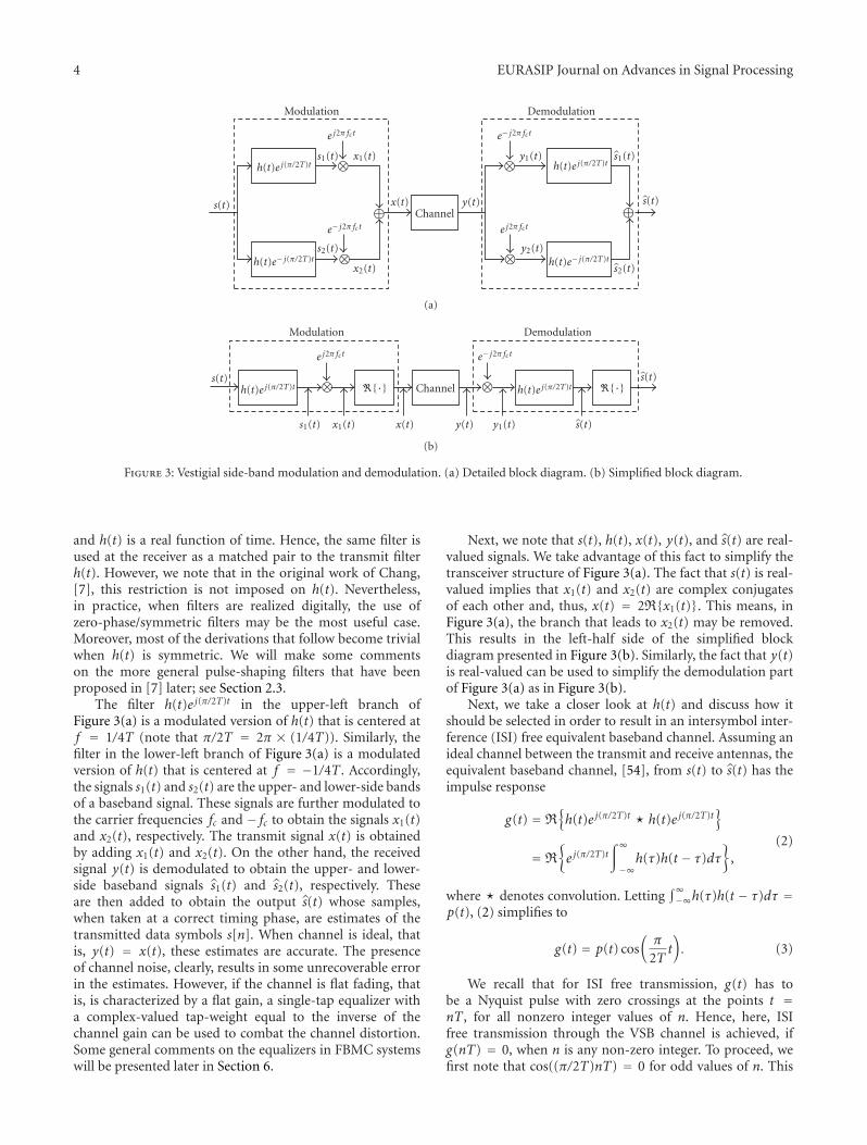
2.1. Vestigial Side-Band Modulation. Figure 2 presents theprocess of taking a baseband signal, modulating it to a VSBchannel, and demodulating the modulated signal back to thebaseband. As shown, for modulation, this process dividesthe spectrum of the baseband signal in two parts, takesone part to modulate a complex sine-wave at the positivefrequency fc (i.e., multiply by e j2π fct) and the other part tomodulate a complex sine-wave at the negative frequency − fc(i.e., multiply by e− j2π fct). Demodulation is performed byreversing these steps.
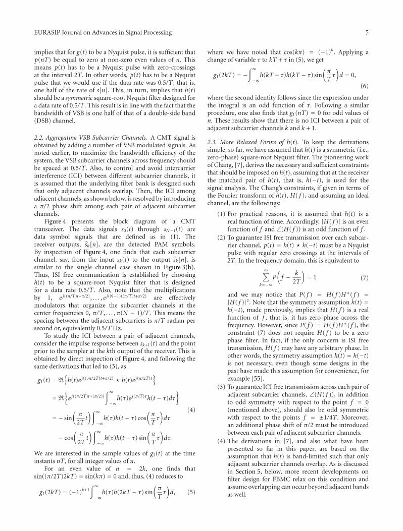
Next, we explain the above steps in a form closely relatedto CMT modulation. Consider the communication systemshown in Figure 3(a). The input signal s(t) is an impulse traincorresponding to a PAM data stream s[n] at the rate of 1/T ,viz.,
s(t) =∞∑
n=−∞s[n]δ(t − nT). (1)
In Figure 3, h(t) is a lowpass filter whose bandwidth is onehalf of the bandwidth of a typical pulse-shaping filter whichone would use for transmission of the data symbols s[n] ata rate of 1/T . We further assume that h(t) is a zero-phasefilter, that is, satisfies the symmetry condition h(−t) = h(t)
4 EURASIP Journal on Advances in Signal Processing
Modulation Demodulation
h(t)e j(π/2T)ts1(t)
e j2π fct
⊗ x1(t) ⊗
s(t)
h(t)e− j(π/2T)ts2(t)⊗
x2(t)
e− j2π fct
x(t)⊕Channel
y(t)
e− j2π fct
y1(t)h(t)e j(π/2T)t
s1(t)
s(t)⊕
e j2π fct
⊗ y2(t)h(t)e− j(π/2T)t
s2(t)
(a)
Modulation Demodulation
h(t)e j(π/2T)t �{·}
e j2π fct
�{·}⊗
x1(t)s1(t)
⊗s(t)
x(t)
Channel
y(t)
e− j2π fct
h(t)e j(π/2T)ts(t)
s(t)y1(t)
(b)
Figure 3: Vestigial side-band modulation and demodulation. (a) Detailed block diagram. (b) Simplified block diagram.
and h(t) is a real function of time. Hence, the same filter isused at the receiver as a matched pair to the transmit filterh(t). However, we note that in the original work of Chang,[7], this restriction is not imposed on h(t). Nevertheless,in practice, when filters are realized digitally, the use ofzero-phase/symmetric filters may be the most useful case.Moreover, most of the derivations that follow become trivialwhen h(t) is symmetric. We will make some commentson the more general pulse-shaping filters that have beenproposed in [7] later; see Section 2.3.
The filter h(t)e j(π/2T)t in the upper-left branch ofFigure 3(a) is a modulated version of h(t) that is centered atf = 1/4T (note that π/2T = 2π × (1/4T)). Similarly, thefilter in the lower-left branch of Figure 3(a) is a modulatedversion of h(t) that is centered at f = −1/4T . Accordingly,the signals s1(t) and s2(t) are the upper- and lower-side bandsof a baseband signal. These signals are further modulated tothe carrier frequencies fc and − fc to obtain the signals x1(t)and x2(t), respectively. The transmit signal x(t) is obtainedby adding x1(t) and x2(t). On the other hand, the receivedsignal y(t) is demodulated to obtain the upper- and lower-side baseband signals s1(t) and s2(t), respectively. Theseare then added to obtain the output s(t) whose samples,when taken at a correct timing phase, are estimates of thetransmitted data symbols s[n]. When channel is ideal, thatis, y(t) = x(t), these estimates are accurate. The presenceof channel noise, clearly, results in some unrecoverable errorin the estimates. However, if the channel is flat fading, thatis, is characterized by a flat gain, a single-tap equalizer witha complex-valued tap-weight equal to the inverse of thechannel gain can be used to combat the channel distortion.Some general comments on the equalizers in FBMC systemswill be presented later in Section 6.
Next, we note that s(t), h(t), x(t), y(t), and s(t) are real-valued signals. We take advantage of this fact to simplify thetransceiver structure of Figure 3(a). The fact that s(t) is real-valued implies that x1(t) and x2(t) are complex conjugatesof each other and, thus, x(t) = 2R{x1(t)}. This means, inFigure 3(a), the branch that leads to x2(t) may be removed.This results in the left-half side of the simplified blockdiagram presented in Figure 3(b). Similarly, the fact that y(t)is real-valued can be used to simplify the demodulation partof Figure 3(a) as in Figure 3(b).
Next, we take a closer look at h(t) and discuss how itshould be selected in order to result in an intersymbol inter-ference (ISI) free equivalent baseband channel. Assuming anideal channel between the transmit and receive antennas, theequivalent baseband channel, [54], from s(t) to s(t) has theimpulse response
g(t) = R{h(t)e j(π/2T)t � h(t)e j(π/2T)t
}
= R
{e j(π/2T)t
∫∞
−∞h(τ)h(t − τ)dτ
},
(2)
where � denotes convolution. Letting∫∞−∞h(τ)h(t − τ)dτ =
p(t), (2) simplifies to
g(t) = p(t) cos(π
2Tt). (3)
We recall that for ISI free transmission, g(t) has tobe a Nyquist pulse with zero crossings at the points t =nT , for all nonzero integer values of n. Hence, here, ISIfree transmission through the VSB channel is achieved, ifg(nT) = 0, when n is any non-zero integer. To proceed, wefirst note that cos((π/2T)nT) = 0 for odd values of n. This
EURASIP Journal on Advances in Signal Processing 5
implies that for g(t) to be a Nyquist pulse, it is sufficient thatp(nT) be equal to zero at non-zero even values of n. Thismeans p(t) has to be a Nyquist pulse with zero-crossingsat the interval 2T . In other words, p(t) has to be a Nyquistpulse that we would use if the data rate was 0.5/T , that is,one half of the rate of s[n]. This, in turn, implies that h(t)should be a symmetric square-root Nyquist filter designed fora data rate of 0.5/T . This result is in line with the fact that thebandwidth of VSB is one half of that of a double-side band(DSB) channel.
2.2. Aggregating VSB Subcarrier Channels. A CMT signal isobtained by adding a number of VSB modulated signals. Asnoted earlier, to maximize the bandwidth efficiency of thesystem, the VSB subcarrier channels across frequency shouldbe spaced at 0.5/T . Also, to control and avoid intercarrierinterference (ICI) between different subcarrier channels, itis assumed that the underlying filter bank is designed suchthat only adjacent channels overlap. Then, the ICI amongadjacent channels, as shown below, is resolved by introducinga π/2 phase shift among each pair of adjacent subcarrierchannels.
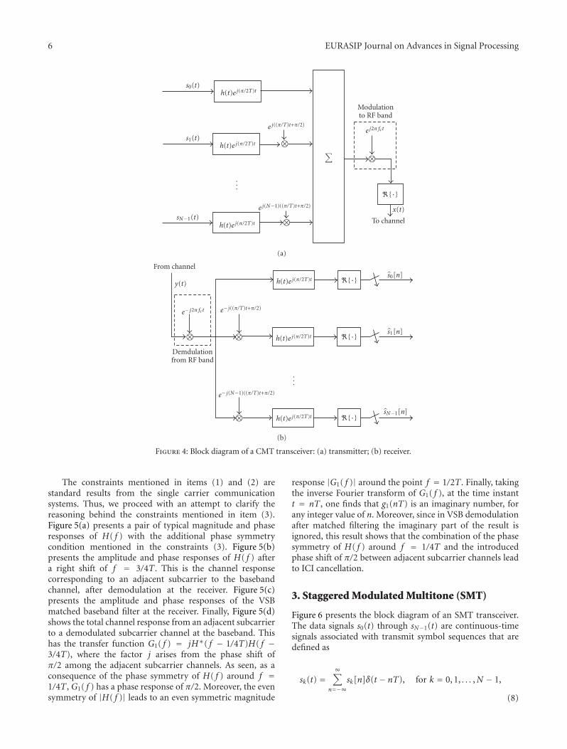
Figure 4 presents the block diagram of a CMTtransceiver. The data signals s0(t) through sN−1(t) aredata symbol signals that are defined as in (1). Thereceiver outputs, sk[n], are the detected PAM symbols.By inspection of Figure 4, one finds that each subcarrierchannel, say, from the input sk(t) to the output sk[n], issimilar to the single channel case shown in Figure 3(b).Thus, ISI free communication is established by choosingh(t) to be a square-root Nyquist filter that is designedfor a data rate 0.5/T . Also, note that the multiplicationsby 1, e j((π/T)t+π/2), . . . , e j(N−1)((π/T)t+π/2) are effectivelymodulators that organize the subcarrier channels at thecenter frequencies 0, π/T , . . . ,π(N − 1)/T . This means thespacing between the adjacent subcarriers is π/T radian persecond or, equivalently 0.5/T Hz.
To study the ICI between a pair of adjacent channels,consider the impulse response between sk+1(t) and the pointprior to the sampler at the kth output of the receiver. This isobtained by direct inspection of Figure 4, and following thesame derivations that led to (3), as
g1(t) = R{h(t)e j((3π/2T)t+π/2) � h(t)e j(π/2T)t
}
= R
{e j((π/2T)t+(π/2))
∫∞
−∞h(τ)e j(π/T)τh(t − τ)dτ
}
= − sin(π
2Tt)∫∞
−∞h(τ)h(t − τ) cos
(π
Tτ)dτ
− cos(π
2Tt)∫∞
−∞h(τ)h(t − τ) sin
(π
Tτ)dτ.
(4)
We are interested in the sample values of g1(t) at the timeinstants nT , for all integer values of n.
For an even value of n = 2k, one finds thatsin((π/2T)2kT) = sin(kπ) = 0 and, thus, (4) reduces to
g1(2kT) = (−1)k+1∫∞
−∞h(τ)h(2kT − τ) sin
(π
Tτ)d, (5)
where we have noted that cos(kπ) = (−1)k. Applying achange of variable τ to kT + τ in (5), we get
g1(2kT) = −∫∞
−∞h(kT + τ)h(kT − τ) sin
(π
Tτ)d = 0,
(6)
where the second identity follows since the expression underthe integral is an odd function of τ. Following a similarprocedure, one also finds that g1(nT) = 0 for odd values ofn. These results show that there is no ICI between a pair ofadjacent subcarrier channels k and k + 1.
2.3. More Relaxed Forms of h(t). To keep the derivationssimple, so far, we have assumed that h(t) is a symmetric (i.e.,zero-phase) square-root Nyquist filter. The pioneering workof Chang, [7], derives the necessary and sufficient constraintsthat should be imposed on h(t), assuming that at the receiverthe matched pair of h(t), that is, h(−t), is used for thesignal analysis. The Chang’s constraints, if given in terms ofthe Fourier transform of h(t), H( f ), and assuming an idealchannel, are the followings:
(1) For practical reasons, it is assumed that h(t) is areal function of time. Accordingly, |H( f )| is an evenfunction of f and ∠(H( f )) is an odd function of f .
(2) To guarantee ISI free transmission over each subcar-rier channel, p(t) = h(t)� h(−t) must be a Nyquistpulse with regular zero crossings at the intervals of2T . In the frequency domain, this is equivalent to
∞∑
k=−∞P(f − k
2T
)= 1 (7)
and we may notice that P( f ) = H( f )H∗( f ) =|H( f )|2. Note that the symmetry assumption h(t) =h(−t), made previously, implies that H( f ) is a realfunction of f , that is, it has zero phase across thefrequency. However, since P( f ) = H( f )H∗( f ), theconstraint (7) does not require H( f ) to be a zerophase filter. In fact, if the only concern is ISI freetransmission, H( f ) may have any arbitrary phase. Inother words, the symmetry assumption h(t) = h(−t)is not necessary, even though some designs in thepast have made this assumption for convenience, forexample [55].
(3) To guarantee ICI free transmission across each pair ofadjacent subcarrier channels, ∠(H( f )), in additionto odd symmetry with respect to the point f = 0(mentioned above), should also be odd symmetricwith respect to the points f = ±1/4T . Moreover,an additional phase shift of π/2 must be introducedbetween each pair of adjacent subcarrier channels.
(4) The derivations in [7], and also what have beenpresented so far in this paper, are based on theassumption that h(t) is band-limited such that onlyadjacent subcarrier channels overlap. As is discussedin Section 5, below, more recent developments onfilter design for FBMC relax on this condition andassume overlapping can occur beyond adjacent bandsas well.
6 EURASIP Journal on Advances in Signal Processing
s0(t)h(t)e j(π/2T)t
s1(t)
sN−1(t)h(t)e j(π/2T)t
h(t)e j(π/2T)t⊗
⊗
e j((π/T)t+π/2)
...
e j(N−1)((π/T)t+π/2)
∑
e j2π fct
Modulationto RF band
⊗
�{·}
x(t)
To channel
(a)
h(t)e j(π/2T)ty(t)
h(t)e j(π/2T)t
h(t)e j(π/2T)t⊗ ⊗
e− j2π fct
...
e− j(N−1)((π/T)t+π/2)
e− j((π/T)t+π/2)
Demdulationfrom RF band
⊗ �{·}
�{·}
�{·}
sN−1[n]
s1[n]
s0[n]From channel
(b)
Figure 4: Block diagram of a CMT transceiver: (a) transmitter; (b) receiver.
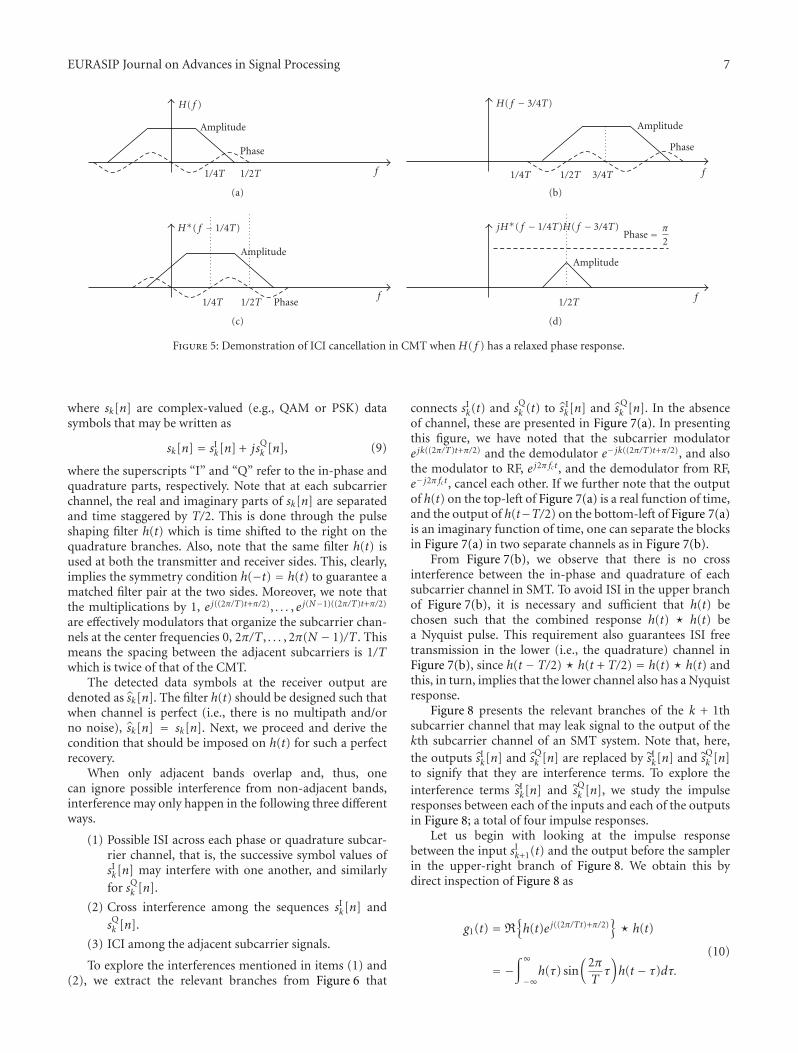
The constraints mentioned in items (1) and (2) arestandard results from the single carrier communicationsystems. Thus, we proceed with an attempt to clarify thereasoning behind the constraints mentioned in item (3).Figure 5(a) presents a pair of typical magnitude and phaseresponses of H( f ) with the additional phase symmetrycondition mentioned in the constraints (3). Figure 5(b)presents the amplitude and phase responses of H( f ) aftera right shift of f = 3/4T . This is the channel responsecorresponding to an adjacent subcarrier to the basebandchannel, after demodulation at the receiver. Figure 5(c)presents the amplitude and phase responses of the VSBmatched baseband filter at the receiver. Finally, Figure 5(d)shows the total channel response from an adjacent subcarrierto a demodulated subcarrier channel at the baseband. Thishas the transfer function G1( f ) = jH∗( f − 1/4T)H( f −3/4T), where the factor j arises from the phase shift ofπ/2 among the adjacent subcarrier channels. As seen, as aconsequence of the phase symmetry of H( f ) around f =1/4T , G1( f ) has a phase response of π/2. Moreover, the evensymmetry of |H( f )| leads to an even symmetric magnitude
response |G1( f )| around the point f = 1/2T . Finally, takingthe inverse Fourier transform of G1( f ), at the time instantt = nT , one finds that g1(nT) is an imaginary number, forany integer value of n. Moreover, since in VSB demodulationafter matched filtering the imaginary part of the result isignored, this result shows that the combination of the phasesymmetry of H( f ) around f = 1/4T and the introducedphase shift of π/2 between adjacent subcarrier channels leadto ICI cancellation.
3. Staggered Modulated Multitone (SMT)
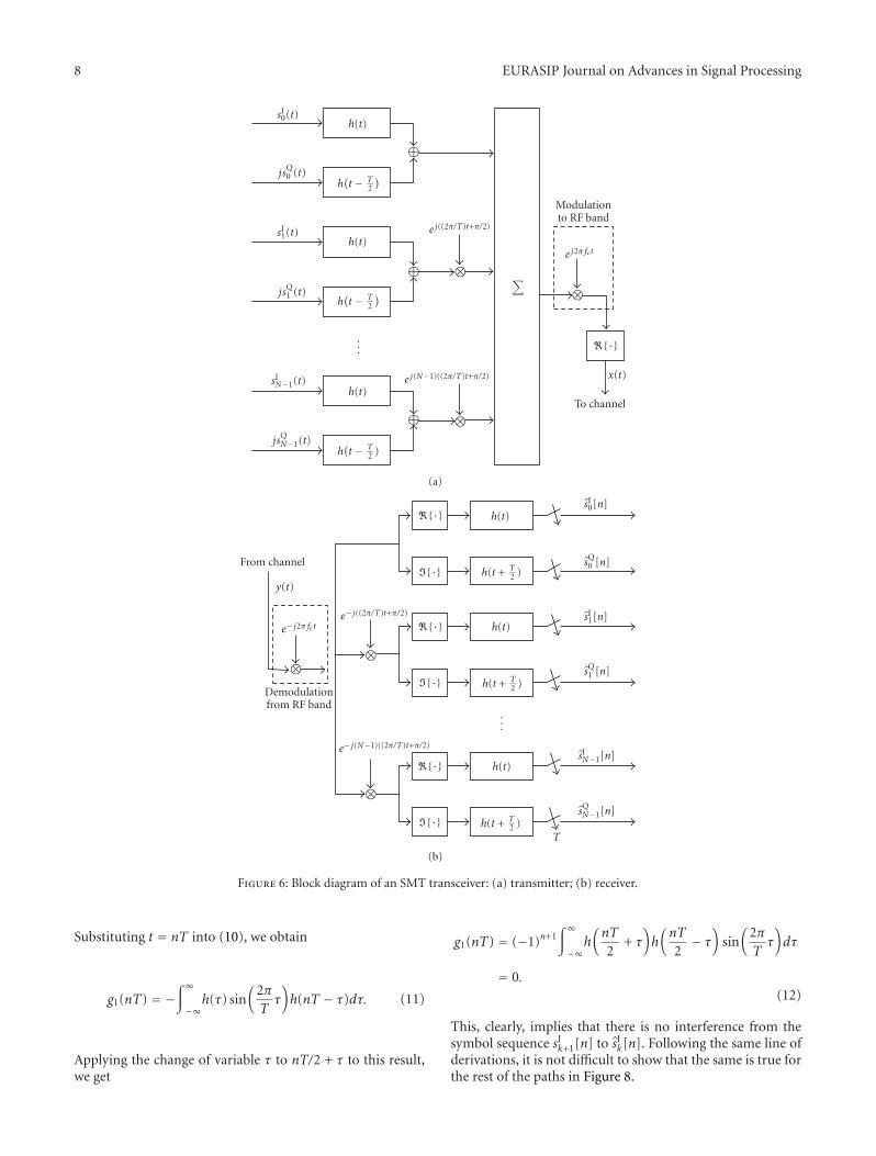
Figure 6 presents the block diagram of an SMT transceiver.The data signals s0(t) through sN−1(t) are continuous-timesignals associated with transmit symbol sequences that aredefined as
sk(t) =∞∑
n=−∞sk[n]δ(t − nT), for k = 0, 1, . . . ,N − 1,
(8)
EURASIP Journal on Advances in Signal Processing 7
H( f )
Amplitude
Phase
f1/4T 1/2T
(a)
H( f − 3/4T)
Amplitude
Phase
f1/4T 1/2T 3/4T
(b)
H∗( f − 1/4T)
Amplitude
Phasef
1/4T 1/2T
(c)
jH∗( f − 1/4T)H( f − 3/4T)
Amplitude
Phase = π
2
f1/2T
(d)
Figure 5: Demonstration of ICI cancellation in CMT when H( f ) has a relaxed phase response.
where sk[n] are complex-valued (e.g., QAM or PSK) datasymbols that may be written as
sk[n] = sIk[n] + jsQk [n], (9)
where the superscripts “I” and “Q” refer to the in-phase andquadrature parts, respectively. Note that at each subcarrierchannel, the real and imaginary parts of sk[n] are separatedand time staggered by T/2. This is done through the pulseshaping filter h(t) which is time shifted to the right on thequadrature branches. Also, note that the same filter h(t) isused at both the transmitter and receiver sides. This, clearly,implies the symmetry condition h(−t) = h(t) to guarantee amatched filter pair at the two sides. Moreover, we note thatthe multiplications by 1, e j((2π/T)t+π/2), . . . , e j(N−1)((2π/T)t+π/2)
are effectively modulators that organize the subcarrier chan-nels at the center frequencies 0, 2π/T , . . . , 2π(N − 1)/T . Thismeans the spacing between the adjacent subcarriers is 1/Twhich is twice of that of the CMT.
The detected data symbols at the receiver output aredenoted as sk[n]. The filter h(t) should be designed such thatwhen channel is perfect (i.e., there is no multipath and/orno noise), sk[n] = sk[n]. Next, we proceed and derive thecondition that should be imposed on h(t) for such a perfectrecovery.
When only adjacent bands overlap and, thus, onecan ignore possible interference from non-adjacent bands,interference may only happen in the following three differentways.
(1) Possible ISI across each phase or quadrature subcar-rier channel, that is, the successive symbol values ofsIk[n] may interfere with one another, and similarly
for sQk [n].
(2) Cross interference among the sequences sIk[n] and
sQk [n].
(3) ICI among the adjacent subcarrier signals.
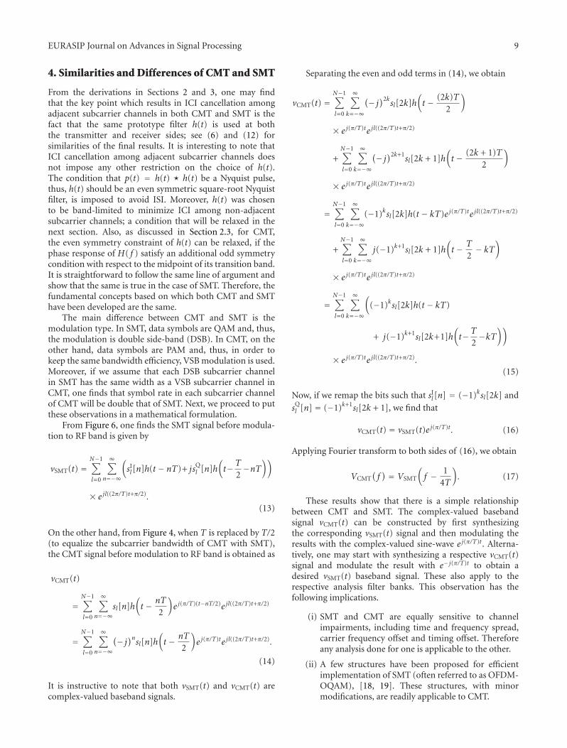
To explore the interferences mentioned in items (1) and(2), we extract the relevant branches from Figure 6 that
connects sIk(t) and sQk (t) to s Ik[n] and sQ
k [n]. In the absenceof channel, these are presented in Figure 7(a). In presentingthis figure, we have noted that the subcarrier modulatore jk((2π/T)t+π/2) and the demodulator e− jk((2π/T)t+π/2), and alsothe modulator to RF, e j2π fct, and the demodulator from RF,e− j2π fct, cancel each other. If we further note that the outputof h(t) on the top-left of Figure 7(a) is a real function of time,and the output of h(t−T/2) on the bottom-left of Figure 7(a)is an imaginary function of time, one can separate the blocksin Figure 7(a) in two separate channels as in Figure 7(b).
From Figure 7(b), we observe that there is no crossinterference between the in-phase and quadrature of eachsubcarrier channel in SMT. To avoid ISI in the upper branchof Figure 7(b), it is necessary and sufficient that h(t) bechosen such that the combined response h(t) � h(t) bea Nyquist pulse. This requirement also guarantees ISI freetransmission in the lower (i.e., the quadrature) channel inFigure 7(b), since h(t − T/2)� h(t + T/2) = h(t)� h(t) andthis, in turn, implies that the lower channel also has a Nyquistresponse.
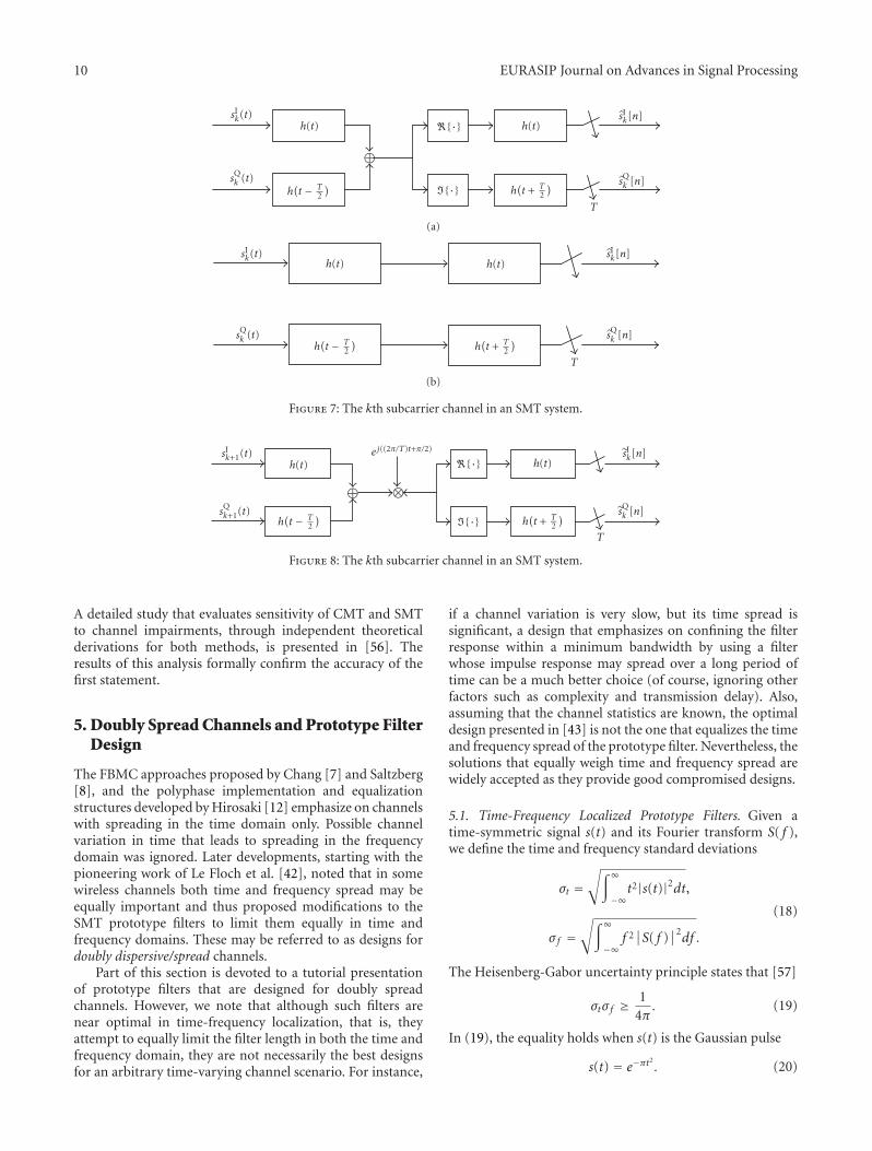
Figure 8 presents the relevant branches of the k + 1thsubcarrier channel that may leak signal to the output of thekth subcarrier channel of an SMT system. Note that, here,the outputs sIk[n] and sQk [n] are replaced by sIk[n] and sQk [n]to signify that they are interference terms. To explore theinterference terms sIk[n] and sQk [n], we study the impulseresponses between each of the inputs and each of the outputsin Figure 8; a total of four impulse responses.
Let us begin with looking at the impulse responsebetween the input sIk+1(t) and the output before the samplerin the upper-right branch of Figure 8. We obtain this bydirect inspection of Figure 8 as
g1(t) = R{h(t)e j((2π/Tt)+π/2)
}� h(t)
= −∫∞
−∞h(τ) sin
(2πTτ)h(t − τ)dτ.
(10)
8 EURASIP Journal on Advances in Signal Processing
sI0(t)
jsQ0 (t)
sI1(t)
jsQ1 (t)
...
sIN−1(t)
jsQN−1(t)
h(t)
h(t − T
2
)
h(t)
h(t − T
2
)
h(t)
h(t − T
2 )
⊕
e j((2π/T)t+π/2)
⊕ ⊗
⊗
⊗
e j2π fct
∑
e j(N−1)((2π/T)t+π/2)
⊕
Modulationto RF band
�{·}
x(t)
To channel
(a)
sI0[n]
sQ0 [n]
sI1[n]
sQ1 [n]
sIN−1[n]
sQN−1[n]
h(t)
�{·}T
�{·}
�{·}
�{·}
�{·}
...
�{·}
h(t + T2 )
h(t)
h(t + T2 )
h(t)
h(t + T2 )
e− j((2π/T)t+π/2)
e− j2π fct
⊗⊗
⊗
e− j(N−1)((2π/T)t+π/2)
Demodulationfrom RF band
y(t)
From channel
(b)
Figure 6: Block diagram of an SMT transceiver: (a) transmitter; (b) receiver.
Substituting t = nT into (10), we obtain
g1(nT) = −∫∞
−∞h(τ) sin
(2πTτ)h(nT − τ)dτ. (11)
Applying the change of variable τ to nT/2 + τ to this result,we get
g1(nT) = (−1)n+1∫∞
−∞h(nT
2+ τ)h(nT
2− τ)
sin(
2πTτ)dτ
= 0.(12)
This, clearly, implies that there is no interference from thesymbol sequence sIk+1[n] to sIk[n]. Following the same line ofderivations, it is not difficult to show that the same is true forthe rest of the paths in Figure 8.
EURASIP Journal on Advances in Signal Processing 9
4. Similarities and Differences of CMT and SMT
From the derivations in Sections 2 and 3, one may findthat the key point which results in ICI cancellation amongadjacent subcarrier channels in both CMT and SMT is thefact that the same prototype filter h(t) is used at boththe transmitter and receiver sides; see (6) and (12) forsimilarities of the final results. It is interesting to note thatICI cancellation among adjacent subcarrier channels doesnot impose any other restriction on the choice of h(t).The condition that p(t) = h(t) � h(t) be a Nyquist pulse,thus, h(t) should be an even symmetric square-root Nyquistfilter, is imposed to avoid ISI. Moreover, h(t) was chosento be band-limited to minimize ICI among non-adjacentsubcarrier channels; a condition that will be relaxed in thenext section. Also, as discussed in Section 2.3, for CMT,the even symmetry constraint of h(t) can be relaxed, if thephase response of H( f ) satisfy an additional odd symmetrycondition with respect to the midpoint of its transition band.It is straightforward to follow the same line of argument andshow that the same is true in the case of SMT. Therefore, thefundamental concepts based on which both CMT and SMThave been developed are the same.
The main difference between CMT and SMT is themodulation type. In SMT, data symbols are QAM and, thus,the modulation is double side-band (DSB). In CMT, on theother hand, data symbols are PAM and, thus, in order tokeep the same bandwidth efficiency, VSB modulation is used.Moreover, if we assume that each DSB subcarrier channelin SMT has the same width as a VSB subcarrier channel inCMT, one finds that symbol rate in each subcarrier channelof CMT will be double that of SMT. Next, we proceed to putthese observations in a mathematical formulation.
From Figure 6, one finds the SMT signal before modula-tion to RF band is given by
vSMT(t) =N−1∑
l=0
∞∑
n=−∞
(sIl[n]h(t − nT)+ jsQl [n]h
(t−T
2−nT
))
× e jl((2π/T)t+π/2).(13)
On the other hand, from Figure 4, when T is replaced by T/2(to equalize the subcarrier bandwidth of CMT with SMT),the CMT signal before modulation to RF band is obtained as
vCMT(t)
=N−1∑
l=0
∞∑
n=−∞sl[n]h
(t − nT
2
)e j(π/T)(t−nT/2)e jl((2π/T)t+π/2)
=N−1∑
l=0
∞∑
n=−∞
(− j)nsl[n]h(t − nT
2
)e j(π/T)te jl((2π/T)t+π/2).
(14)
It is instructive to note that both vSMT(t) and vCMT(t) arecomplex-valued baseband signals.
Separating the even and odd terms in (14), we obtain
vCMT(t) =N−1∑
l=0
∞∑
k=−∞
(− j)2ksl[2k]h
(t − (2k)T
2
)
× e j(π/T)te jl((2π/T)t+π/2)
+N−1∑
l=0
∞∑
k=−∞
(− j)2k+1sl[2k + 1]h
(t − (2k + 1)T
2
)
× e j(π/T)te jl((2π/T)t+π/2)
=N−1∑
l=0
∞∑
k=−∞(−1)ksl[2k]h(t − kT)e j(π/T)te jl((2π/T)t+π/2)
+N−1∑
l=0
∞∑
k=−∞j(−1)k+1sl[2k + 1]h
(t − T
2− kT
)
× e j(π/T)te jl((2π/T)t+π/2)
=N−1∑
l=0
∞∑
k=−∞
((−1)ksl[2k]h(t − kT)
+ j(−1)k+1sl[2k+1]h(t−T
2−kT
))
× e j(π/T)te jl((2π/T)t+π/2).(15)
Now, if we remap the bits such that sIl [n] = (−1)ksl[2k] and
sQl [n] = (−1)k+1sl[2k + 1], we find that
vCMT(t) = vSMT(t)e j(π/T)t . (16)
Applying Fourier transform to both sides of (16), we obtain
VCMT(f) = VSMT
(f − 1
4T
). (17)
These results show that there is a simple relationshipbetween CMT and SMT. The complex-valued basebandsignal vCMT(t) can be constructed by first synthesizingthe corresponding vSMT(t) signal and then modulating theresults with the complex-valued sine-wave e j(π/T)t. Alterna-tively, one may start with synthesizing a respective vCMT(t)signal and modulate the result with e− j(π/T)t to obtain adesired vSMT(t) baseband signal. These also apply to therespective analysis filter banks. This observation has thefollowing implications.
(i) SMT and CMT are equally sensitive to channelimpairments, including time and frequency spread,carrier frequency offset and timing offset. Thereforeany analysis done for one is applicable to the other.
(ii) A few structures have been proposed for efficientimplementation of SMT (often referred to as OFDM-OQAM), [18, 19]. These structures, with minormodifications, are readily applicable to CMT.
10 EURASIP Journal on Advances in Signal Processing
h(t − T
2
)
h(t)
h(t + T
2
)
h(t)
⊕
�{·}
�{·}sIk(t)
sQk (t)
sIk[n]
sQk [n]
T
(a)
h(t − T
2
)
h(t)
h(t + T
2
)
h(t)sIk(t)
sQk (t)
sIk[n]
sQk [n]
T
(b)
Figure 7: The kth subcarrier channel in an SMT system.
h(t − T
2
)
h(t)
h(t + T
2
)
h(t)e j((2π/T)t+π/2)
⊗⊕
�{·}
�{·}sIk+1(t)
sQk+1(t)
sIk[n]
sQk [n]
T
Figure 8: The kth subcarrier channel in an SMT system.
A detailed study that evaluates sensitivity of CMT and SMTto channel impairments, through independent theoreticalderivations for both methods, is presented in [56]. Theresults of this analysis formally confirm the accuracy of thefirst statement.
5. Doubly Spread Channels and Prototype FilterDesign
The FBMC approaches proposed by Chang [7] and Saltzberg[8], and the polyphase implementation and equalizationstructures developed by Hirosaki [12] emphasize on channelswith spreading in the time domain only. Possible channelvariation in time that leads to spreading in the frequencydomain was ignored. Later developments, starting with thepioneering work of Le Floch et al. [42], noted that in somewireless channels both time and frequency spread may beequally important and thus proposed modifications to theSMT prototype filters to limit them equally in time andfrequency domains. These may be referred to as designs fordoubly dispersive/spread channels.
Part of this section is devoted to a tutorial presentationof prototype filters that are designed for doubly spreadchannels. However, we note that although such filters arenear optimal in time-frequency localization, that is, theyattempt to equally limit the filter length in both the time andfrequency domain, they are not necessarily the best designsfor an arbitrary time-varying channel scenario. For instance,
if a channel variation is very slow, but its time spread issignificant, a design that emphasizes on confining the filterresponse within a minimum bandwidth by using a filterwhose impulse response may spread over a long period oftime can be a much better choice (of course, ignoring otherfactors such as complexity and transmission delay). Also,assuming that the channel statistics are known, the optimaldesign presented in [43] is not the one that equalizes the timeand frequency spread of the prototype filter. Nevertheless, thesolutions that equally weigh time and frequency spread arewidely accepted as they provide good compromised designs.
5.1. Time-Frequency Localized Prototype Filters. Given atime-symmetric signal s(t) and its Fourier transform S( f ),we define the time and frequency standard deviations
σt =√∫∞
−∞t2|s(t)|2dt,
σ f =√∫∞
−∞f 2∣∣S( f )
∣∣2df .
(18)
The Heisenberg-Gabor uncertainty principle states that [57]
σtσ f ≥ 14π
. (19)
In (19), the equality holds when s(t) is the Gaussian pulse
s(t) = e−πt2. (20)
EURASIP Journal on Advances in Signal Processing 11
Also, the Gaussian pulse s(t) has the interesting propertythat S( f ) = s( f ), that is, it is the same function in bothtime and frequency domains. Thus, any deviation from theGaussian pulse, say, to reduce σt, that is, spreading of thesignal in the time domain, will result in an increase ofσ f , that is, spreading in the frequency domain. Therefore,the Gaussian pulse (20) is optimal in the sense that itminimizes the time-frequency product σtσ f and also satisfiesthe desirable property of equal spreading in both time andfrequency domain. However, unfortunately, the Gaussianpulse does not satisfy the Nyquist and other properties ofh(t) which were stated in Sections 2 and 3 for ISI and ICIcancellation in CMT and SMT systems. Noting this, Le Flochet al. [42] and Haas and Belfiore [44] have proposed twodifferent methods for designing pulse shapes that satisfy theconditions necessary for ISI and ICI cancellation in CMTand SMT and result in a time-frequency product that is onlyslightly greater than the lower limit given by (19).
Both design methods in [42, 44] are developed using thetime-frequency ambiguity function
A(τ, f
) =∫∞
−∞h(t)h(t + τ)e− j2π f tdt. (21)
The ambiguity function A(τ, f ) has the following interpreta-tion. For f = 0,
A(τ, 0) =∫∞
−∞h(t)h(t + τ)dt = h(τ)� h(−τ) (22)
and the constraints A(nT , 0) = 0, for n /= 0, imply that h(t)is a square-root Nyquist filter, hence, a sequence of datasymbols that are T spaced can be received free of ISI. Onthe other hand, the constraints A(0, kΔ f ) = 0, for anyk, imply that a pair of modulated filters that are spacedacross frequency by kΔ f do not introduce ICI on each other.Accordingly, if an FBMC system is constructed based on aprototype filter h(t) whose ambiguity function satisfies theconstraints
A(nT , kΔ f
) = 0, for n /= 0, and any k, (23)
where T is the symbol spacing and Δ f is carrier spacing,in the absence of channel distortion, ISI and ICI freetransmission is achieved.
It has been noted that to achieve a reasonable time-frequency localization which results in a value of σtσ f close tothe lower limit of 1/4π, TΔ f should be given a value greaterthan 1 [42, 44]. On the other hand, TΔ f = 2 turns out tobe a good choice as it results in prototype filters with a valueof σtσ f close to the lower limit 1/4π and also, as discussedbelow, is the choice that leads to CMT and SMT systems.
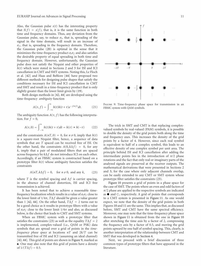
When an FBMC system with a prototype filter thatsatisfies the constraints (23) as well as the equality TΔ f = 2is implemented, complex-valued (i.e., QAM or PSK) datasymbols that are spread over a grid of points in the time-frequency phase space at locations nT and 2k/T can betransmitted free of ISI and ICI (assuming an ideal channel)[42, 44]. This grid of points are shown in Figure 9, marked as
. One may also note that this grid of points have a densityof 1/(TΔ f ) = 0.5.
2T
f
t
−2T −T T 2T
− 2T
Figure 9: Time-frequency phase space for transmission in anFBMC system with QAM symbols.
The trick in SMT and CMT is that replacing complex-valued symbols by real-valued (PAM) symbols, it is possibleto double the density of the grid points both along the timeand frequency axes. This increases the density of the gridpoints by a factor of 4. However, since each real symbolis equivalent to half of a complex symbol, this leads to aneffective density of one complex symbol per unit area. Theprinciple behind ISI and ICI cancellation after adding theintermediate points lies in the introduction of π/2 phaserotations and the fact that only real or imaginary parts of theanalyzed signals are preserved at the receiver outputs. Themathematical derivations that were presented in Sections 2and 3, for the case where only adjacent channels overlap,can be easily extended to any CMT or SMT system whoseprototype filter satisfies the constraints (23).
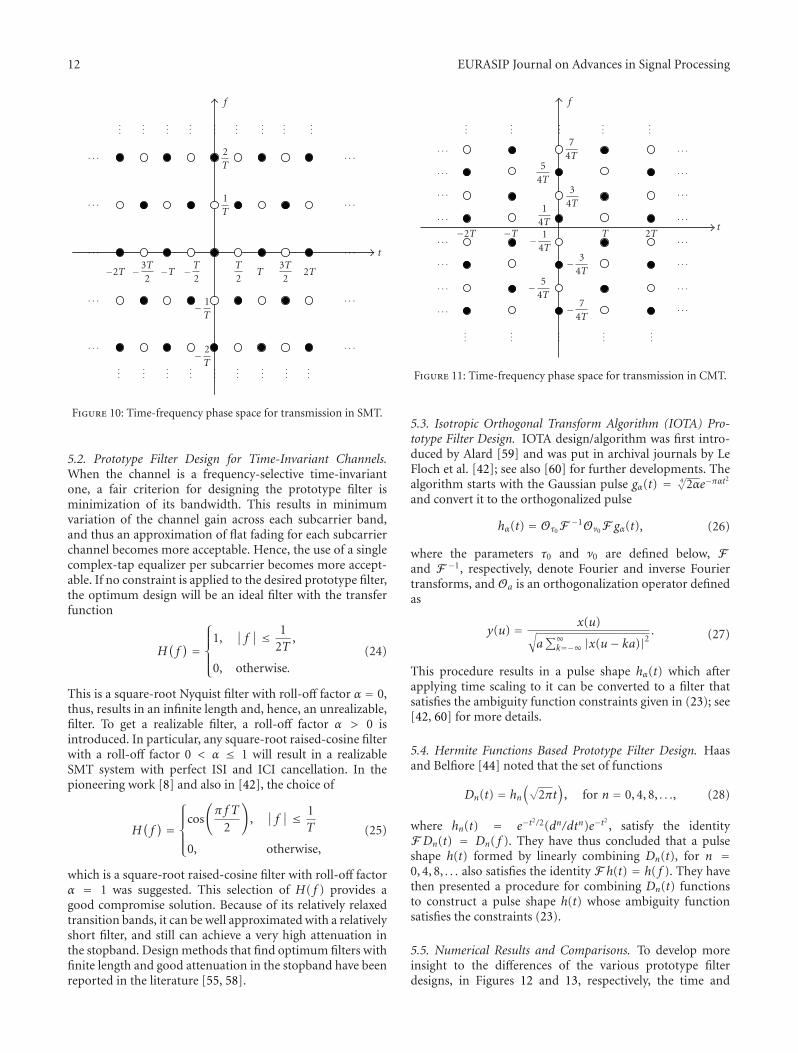
Figure 10 presents a grid of points in a phase space forthe case of SMT. The points where an even and odd factors ofπ/2 phase are applied to the respective symbols are indicatedas and , respectively. A grid of points that correspondsto a CMT system is presented in Figure 11. As one wouldexpect, we note that the density of the grid points in bothFigures 10 and 11 are the same. This implies that, as discussedbefore, SMT and CMT have the same spectral efficiency.Moreover, one may note that the time-frequency phase spaceshown in Figure 11 is obtained from the one in Figure 10after stretching the time axis by a factor of 2, compressingthe frequency axis by a factor of 0.5, and moving the gridpoints upward by one half of symbol spacing. This, clearly, isanother interpretation of the relationship between CMT andSMT that was developed in Section 4.
Next, we proceed with a brief discussion of threecommon types of prototype filters that have appeared in theliterature.
12 EURASIP Journal on Advances in Signal Processing
2T
1T
f
t
−2TT
2−T
2− 3T
2−T T
3T2
2T
− 1T
− 2T
Figure 10: Time-frequency phase space for transmission in SMT.
5.2. Prototype Filter Design for Time-Invariant Channels.When the channel is a frequency-selective time-invariantone, a fair criterion for designing the prototype filter isminimization of its bandwidth. This results in minimumvariation of the channel gain across each subcarrier band,and thus an approximation of flat fading for each subcarrierchannel becomes more acceptable. Hence, the use of a singlecomplex-tap equalizer per subcarrier becomes more accept-able. If no constraint is applied to the desired prototype filter,the optimum design will be an ideal filter with the transferfunction
H(f) =
⎧⎪⎪⎨⎪⎪⎩
1,∣∣ f∣∣ ≤ 1
2T,
0, otherwise.(24)
This is a square-root Nyquist filter with roll-off factor α = 0,thus, results in an infinite length and, hence, an unrealizable,filter. To get a realizable filter, a roll-off factor α > 0 isintroduced. In particular, any square-root raised-cosine filterwith a roll-off factor 0 < α ≤ 1 will result in a realizableSMT system with perfect ISI and ICI cancellation. In thepioneering work [8] and also in [42], the choice of
H(f) =
⎧⎪⎪⎨⎪⎪⎩
cos
(π f T
2
),∣∣ f∣∣ ≤ 1
T
0, otherwise,
(25)
which is a square-root raised-cosine filter with roll-off factorα = 1 was suggested. This selection of H( f ) provides agood compromise solution. Because of its relatively relaxedtransition bands, it can be well approximated with a relativelyshort filter, and still can achieve a very high attenuation inthe stopband. Design methods that find optimum filters withfinite length and good attenuation in the stopband have beenreported in the literature [55, 58].
14T
34T
54T
74T
f
t−2T − 14T
−T T 2T
− 34T
− 54T
− 74T
Figure 11: Time-frequency phase space for transmission in CMT.
5.3. Isotropic Orthogonal Transform Algorithm (IOTA) Pro-totype Filter Design. IOTA design/algorithm was first intro-duced by Alard [59] and was put in archival journals by LeFloch et al. [42]; see also [60] for further developments. Thealgorithm starts with the Gaussian pulse gα(t) = 4
√2αe−παt
2
and convert it to the orthogonalized pulse
hα(t) = Oτ0F−1Oν0F gα(t), (26)
where the parameters τ0 and ν0 are defined below, Fand F −1, respectively, denote Fourier and inverse Fouriertransforms, and Oa is an orthogonalization operator definedas
y(u) = x(u)√a∑∞
k=−∞ |x(u− ka)|2. (27)
This procedure results in a pulse shape hα(t) which afterapplying time scaling to it can be converted to a filter thatsatisfies the ambiguity function constraints given in (23); see[42, 60] for more details.
5.4. Hermite Functions Based Prototype Filter Design. Haasand Belfiore [44] noted that the set of functions
Dn(t) = hn(√
2πt)
, for n = 0, 4, 8, . . ., (28)
where hn(t) = e−t2/2(dn/dtn)e−t
2, satisfy the identity
F Dn(t) = Dn( f ). They have thus concluded that a pulseshape h(t) formed by linearly combining Dn(t), for n =0, 4, 8, . . . also satisfies the identity F h(t) = h( f ). They havethen presented a procedure for combining Dn(t) functionsto construct a pulse shape h(t) whose ambiguity functionsatisfies the constraints (23).
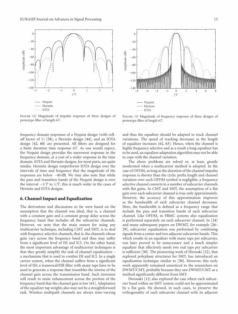
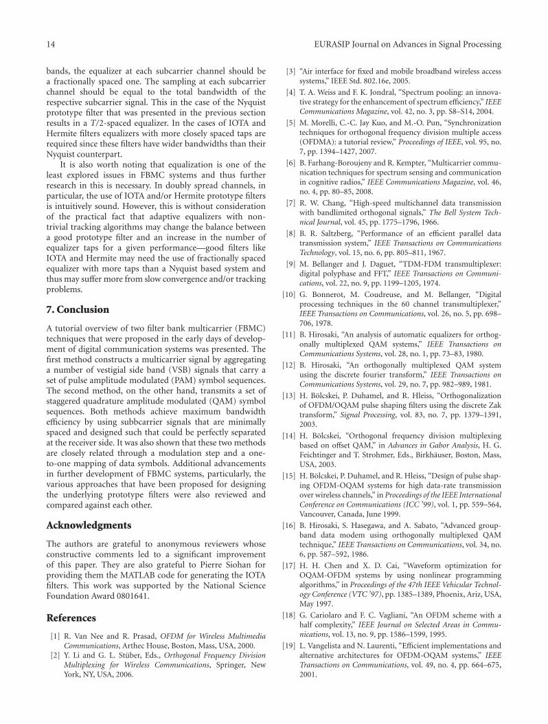
5.5. Numerical Results and Comparisons. To develop moreinsight to the differences of the various prototype filterdesigns, in Figures 12 and 13, respectively, the time and
EURASIP Journal on Advances in Signal Processing 13
−140
−120
−100
−80
Am
plit
ude
(dB
)
−60
−40
−20
0
−3 −2 −1 0 1t/T
2 3
NyquistHermiteIOTA
Figure 12: Magnitude of impulse response of three designs ofprototype filter of length 6T .
frequency domain responses of a Nyquist design (with roll-off factor of 1) [58], a Hermite design [44], and an IOTAdesign [42, 60] are presented. All filters are designed fora finite duration time response 6T . As one would expect,the Nyquist design provides the narrowest response in thefrequency domain, at a cost of a wider response in the timedomain. IOTA and Hermite designs, for most parts, are quitesimilar. Hermite design outperforms IOTA design over theintervals of time and frequency that the magnitude of theresponses are below −40 dB. We may also note that whilethe pass and transition bands of the Nyquist design is overthe interval −1/T to 1/T , this is much wider in the cases ofHermite and IOTA designs.
6. Channel Impact and Equalization
The derivations and discussions so far were based on theassumption that the channel was ideal, that is, a channelwith a constant gain and a constant group delay across thefrequency band that includes all the subcarrier channels.However, we note that the main reason for using anymulticarrier technique, including CMT and SMT, is to dealwith frequency selective channels, that is, the channels whosegain vary across the frequency band and thus may sufferfrom a significant level of ISI and ICI. On the other hand,the most important advantage of multicarrier techniques isthat they greatly simplify the task of channel equalization –a mechanism that is used to combat ISI and ICI. In a singlecarrier system, when the channel suffers from a significantlevel of ISI, a transveral/FIR filter with many taps have to beused to generate a response that resembles the inverse of thechannel gain across the transmission band. Such inversionwill result in noise enhancement across the portion of thefrequency band that the channel gain is low [61]. Adaptationof the equalizer tap weights also may not be a straightforwardtask. Wireless multipath channels are always time-varying
−140
−120
−100
−80
Am
plit
ude
(dB
)
−60
−40
−20
0
−8 −6 −4 −2 0 2f T
4 6 8
NyquistHermiteIOTA
Figure 13: Magnitude of frequency response of three designs ofprototype filter of length 6T .
and thus the equalizer should be adapted to track channelvariations. The speed of tracking decreases as the lengthof equalizer increases [62, 63]. Hence, when the channel ishighly frequency selective and as a result a long equalizer hasto be used, an equalizer adaptation algorithm may not be ableto cope with the channel variation.
The above problems are solved or, at least, greatlymoderated when a multicarrier method is adopted. In thecase of OFDM, as long as the duration of the channel impulseresponse is shorter than the cyclic prefix length and channelvariation over each OFDM symbol is negligible, a frequencyselective channel converts to a number of subcarrier channelswith flat gains. In CMT and SMT, the assumption of a flatgain over each subcarrier channel is true only approximately.However, the accuracy of this approximation improvesas the bandwidth of each subcarrier channel decreases.Here, the bandwidth is defined as a frequency range thatinclude the pass and transition bands of each subcarrierchannel. Like OFDM, in FBMC systems also equalizationis performed separately on each subcarrier channel. In [24]and many subsequent papers on DWMT, for example [26–29], subcarrier equalization was performed by combiningsignals from a center and two adjacent subcarrier bands. Thiswhich results in an equalizer with many taps per subcarrier,was later proved to be unnecessary and a much simplerequalizer that effectively needs two real taps per subcarrieris sufficient [30]. The pioneering work of Hirosaki [12], thatexplored polyphase structures for SMT, has introduced anequalization technique similar to [30]. However, this earlywork apparently remained unnoticed to the researchers onDWMT/CMT, probably because they saw DWMT/CMT as amethod significantly different from SMT.
Horosaki [12] also explored the case where each subcar-rier band within an SMT system could not be approximatedby a flat gain. He showed, in such cases, to preserve theorthogonality of each subcarrier channel with its adjacent
14 EURASIP Journal on Advances in Signal Processing
bands, the equalizer at each subcarrier channel should bea fractionally spaced one. The sampling at each subcarrierchannel should be equal to the total bandwidth of therespective subcarrier signal. This in the case of the Nyquistprototype filter that was presented in the previous sectionresults in a T/2-spaced equalizer. In the cases of IOTA andHermite filters equalizers with more closely spaced taps arerequired since these filters have wider bandwidths than theirNyquist counterpart.
It is also worth noting that equalization is one of theleast explored issues in FBMC systems and thus furtherresearch in this is necessary. In doubly spread channels, inparticular, the use of IOTA and/or Hermite prototype filtersis intuitively sound. However, this is without considerationof the practical fact that adaptive equalizers with non-trivial tracking algorithms may change the balance betweena good prototype filter and an increase in the number ofequalizer taps for a given performance—good filters likeIOTA and Hermite may need the use of fractionally spacedequalizer with more taps than a Nyquist based system andthus may suffer more from slow convergence and/or trackingproblems.
7. Conclusion
A tutorial overview of two filter bank multicarrier (FBMC)techniques that were proposed in the early days of develop-ment of digital communication systems was presented. Thefirst method constructs a multicarrier signal by aggregatinga number of vestigial side band (VSB) signals that carry aset of pulse amplitude modulated (PAM) symbol sequences.The second method, on the other hand, transmits a set ofstaggered quadrature amplitude modulated (QAM) symbolsequences. Both methods achieve maximum bandwidthefficiency by using subbcarrier signals that are minimallyspaced and designed such that could be perfectly separatedat the receiver side. It was also shown that these two methodsare closely related through a modulation step and a one-to-one mapping of data symbols. Additional advancementsin further development of FBMC systems, particularly, thevarious approaches that have been proposed for designingthe underlying prototype filters were also reviewed andcompared against each other.
Acknowledgments
The authors are grateful to anonymous reviewers whoseconstructive comments led to a significant improvementof this paper. They are also grateful to Pierre Siohan forproviding them the MATLAB code for generating the IOTAfilters. This work was supported by the National ScienceFoundation Award 0801641.
References
[1] R. Van Nee and R. Prasad, OFDM for Wireless MultimediaCommunications, Arthec House, Boston, Mass, USA, 2000.
[2] Y. Li and G. L. Stuber, Eds., Orthogonal Frequency DivisionMultiplexing for Wireless Communications, Springer, NewYork, NY, USA, 2006.
[3] “Air interface for fixed and mobile broadband wireless accesssystems,” IEEE Std. 802.16e, 2005.
[4] T. A. Weiss and F. K. Jondral, “Spectrum pooling: an innova-tive strategy for the enhancement of spectrum efficiency,” IEEECommunications Magazine, vol. 42, no. 3, pp. S8–S14, 2004.
[5] M. Morelli, C.-C. Jay Kuo, and M.-O. Pun, “Synchronizationtechniques for orthogonal frequency division multiple access(OFDMA): a tutorial review,” Proceedings of IEEE, vol. 95, no.7, pp. 1394–1427, 2007.
[6] B. Farhang-Boroujeny and R. Kempter, “Multicarrier commu-nication techniques for spectrum sensing and communicationin cognitive radios,” IEEE Communications Magazine, vol. 46,no. 4, pp. 80–85, 2008.
[7] R. W. Chang, “High-speed multichannel data transmissionwith bandlimited orthogonal signals,” The Bell System Tech-nical Journal, vol. 45, pp. 1775–1796, 1966.
[8] B. R. Saltzberg, “Performance of an efficient parallel datatransmission system,” IEEE Transactions on CommunicationsTechnology, vol. 15, no. 6, pp. 805–811, 1967.
[9] M. Bellanger and J. Daguet, “TDM-FDM transmultiplexer:digital polyphase and FFT,” IEEE Transactions on Communi-cations, vol. 22, no. 9, pp. 1199–1205, 1974.
[10] G. Bonnerot, M. Coudreuse, and M. Bellanger, “Digitalprocessing techniques in the 60 channel transmultiplexer,”IEEE Transactions on Communications, vol. 26, no. 5, pp. 698–706, 1978.
[11] B. Hirosaki, “An analysis of automatic equalizers for orthog-onally multiplexed QAM systems,” IEEE Transactions onCommunications Systems, vol. 28, no. 1, pp. 73–83, 1980.
[12] B. Hirosaki, “An orthogonally multiplexed QAM systemusing the discrete fourier transform,” IEEE Transactions onCommunications Systems, vol. 29, no. 7, pp. 982–989, 1981.
[13] H. Bolcskei, P. Duhamel, and R. Hleiss, “Orthogonalizationof OFDM/OQAM pulse shaping filters using the discrete Zaktransform,” Signal Processing, vol. 83, no. 7, pp. 1379–1391,2003.
[14] H. Bolcskei, “Orthogonal frequency division multiplexingbased on offset QAM,” in Advances in Gabor Analysis, H. G.Feichtinger and T. Strohmer, Eds., Birkhauser, Boston, Mass,USA, 2003.
[15] H. Bolcskei, P. Duhamel, and R. Hleiss, “Design of pulse shap-ing OFDM-OQAM systems for high data-rate transmissionover wireless channels,” in Proceedings of the IEEE InternationalConference on Communications (ICC ’99), vol. 1, pp. 559–564,Vancouver, Canada, June 1999.
[16] B. Hirosaki, S. Hasegawa, and A. Sabato, “Advanced group-band data modem using orthogonally multiplexed QAMtechnique,” IEEE Transactions on Communications, vol. 34, no.6, pp. 587–592, 1986.
[17] H. H. Chen and X. D. Cai, “Waveform optimization forOQAM-OFDM systems by using nonlinear programmingalgorithms,” in Proceedings of the 47th IEEE Vehicular Technol-ogy Conference (VTC ’97), pp. 1385–1389, Phoenix, Ariz, USA,May 1997.
[18] G. Cariolaro and F. C. Vagliani, “An OFDM scheme with ahalf complexity,” IEEE Journal on Selected Areas in Commu-nications, vol. 13, no. 9, pp. 1586–1599, 1995.
[19] L. Vangelista and N. Laurenti, “Efficient implementations andalternative architectures for OFDM-OQAM systems,” IEEETransactions on Communications, vol. 49, no. 4, pp. 664–675,2001.
EURASIP Journal on Advances in Signal Processing 15
[20] S. Pfletschinger and J. Speidel, “Optimized impulses formulticarrier offset-QAM,” in Proceedings of the IEEE GlobalTelecommunications Conference (Globecom ’01), pp. 207–211,San Antonio, Texas, USA, November 2001.
[21] P. Siohan, C. Siclet, and N. Lacaille, “Analysis and designof OFDM/OQAM systems based on filterbank theory,” IEEETransactions on Signal Processing, vol. 50, no. 5, pp. 1170–1183,2002.
[22] A. Viholainen, T. Saramaki, and M. Renfors, “Cosine-modulated filter bank design for multicarrier VDSL modems,”in Proceedings of the 6th IEEE International Workshop onIntelligent SP and Communications Systems, pp. 143–147,Melbourne, Australia, November 1998.
[23] M. A. Tzannes, M. C. Tzannes, and H. Resnikoff, “TheDWMT: a multicarrier transceiver for ADSL using M-bandwavelet transforms,” Standards Project ANSI ContributionT1E1.4/93-067, 1993.
[24] M. A. Tzannes, M. C. Tzannes, J. Proakis, and P. N. Heller,“DMT systems, DWMT systems and digital filter banks,” inProceedings of the IEEE International Conference on Commu-nications (SUPERCOMM/ICC ’94), vol. 1, pp. 311–315, NewOrleans, La, USA, May 1994.
[25] S. D. Sandberg and M. A. Tzannes, “Overlapped discretemultitone modulation for high speed copper wire communi-cations,” IEEE Journal on Selected Areas in Communications,vol. 13, no. 9, pp. 1571–1585, 1995.
[26] A. D. Rizos, J. G. Proakis, and T. Q. Nguyen, “Comparison ofDFT and cosine modulated filter banks in multicarrier mod-ulation,” in Proceedings of the IEEE Global TelecommunicationsConference (Globecom ’01), vol. 2, pp. 687–691, San Francisco,Calif, USA, November 1994.
[27] M. Hawryluck, A. Yongacoglu, and M. Kavehrad, “Efficientequalization of discrete wavelet multitone over twisted pair,” inProceedings of the International Zurich Seminar on BroadbandCommunications, pp. 185–191, Zurich, Switzerland, 1998.
[28] S. Govardhanagiri, T. Karp, P. Heller, and T. Nguyen,“Performance analysis of multicarrier modulation systemsusing cosine modulated filter banks,” in Proceedings of theIEEE International Conference on Acoustics, Speech and SignalProcessing (ICASSP ’99), vol. 3, pp. 1405–1408, Phoenix, Ariz,USA, March 1999.
[29] B. Farhang-Boroujeny and W. H. Chin, “Time domainequaliser design for DWMT multicarrier transceivers,” Elec-tronics Letters, vol. 36, no. 18, pp. 1590–1592, 2000.
[30] B. Farhang-Boroujeny, “Multicarrier modulation with blinddetection capability using cosine modulated filter banks,” IEEETransactions on Communications, vol. 51, no. 12, pp. 2057–2070, 2003.
[31] P. P. Vaidyanathan, Multirate Systems and Filter Banks, PrenticeHall, Englewood Cliffs, NJ, USA , 1993.
[32] S. Galli and O. Logvinov, “Recent developments in thestandardization of power line communications within theIEEE,” IEEE Communications Magazine, vol. 46, no. 7, pp. 64–71, 2008.
[33] N. J. Fliege, Multirate Digital Signal Processing, John Wiley &Son, New York, NY, USA, 1994.
[34] N. J. Fliege, “Modified DFT polyphase SBC filter banks withalmost perfect reconstruction,” in Proceedings of the Interna-tional Conference on Acoustics, Speech, and Signal Processing(ICASSP ’94), vol. 3, pp. 149–152, Adelaide, Australia, April1994.
[35] T. Karp and N. J. Fliege, “Modified DFT filter banks withperfect reconstruction,” IEEE Transactions on Circuits andSystems II: Analog and Digital Signal Processing, vol. 46, no. 11,pp. 1404–1414, 1999.
[36] R. Bregovic and T. Saramaki, “A systematic technique fordesigning linear-phase FIR prototype filters for perfect-reconstruction cosine-modulated and modified DFT filter-banks,” IEEE Transactions on Signal Processing, vol. 53, no. 8,pp. 3193–3201, 2005.
[37] S. Salcedo-Sanz, F. Cruz-Roldan, and X. Yao, “Evolutionarydesign of digital filters with application to subband coding anddata transmission,” IEEE Transactions on Signal Processing, vol.55, no. 4, pp. 1193–1203, 2007.
[38] P. N . Heller, T. Karp, and T. Q. Nguyen, “A generalformulation of modulated filter banks,” IEEE Transactions onSignal Processing, vol. 47, no. 4, pp. 986–1002, 1999.
[39] R. D. Gitlin and E. Y. Ho, “The performance of staggeredquadrature amplitude modulation in the presence of phasejitter,” IEEE Transactions on Communications, vol. 23, no. 3,pp. 348–352, 1975.
[40] H. Bolcskei, “Blind estimation of symbol timing and carrierfrequency offset in wireless OFDM systems,” IEEE Transactionson Communications, vol. 49, no. 6, pp. 988–999, 2001.
[41] H. Bolcskei, P. Duhamel, and R. Hleiss, “A subspace-basedapproach to blind channel identification in pulse shapingOFDM/OQAM systems,” IEEE Transactions on Signal Process-ing, vol. 49, no. 7, pp. 1594–1598, 2001.
[42] B. Le Floch, M. Alard, and C. Berrou, “Coded orthogonalfrequency division multiplex,” Proceedings of the IEEE, vol. 83,no. 6, pp. 982–996, 1995.
[43] W. Kozek and A. F. Molisch, “Nonorthogonal pulseshapes formulticarrier communications in doubly dispersive channels,”IEEE Journal on Selected Areas in Communications, vol. 16, no.8, pp. 1579–1589, 1998.
[44] R. Haas and J.-C. Belfiore, “A time-frequency well-localizedpulse for multiple carrier transmission,” Wireless PersonalCommunications, vol. 5, no. 1, pp. 1–18, 1997.
[45] T. Hunziker and D. Dahlhaus, “Iterative detection for multi-carrier transmission employing time-frequency concentratedpulses,” IEEE Transactions on Communications, vol. 51, no. 4,pp. 641–651, 2003.
[46] G. Matz, D. Schafhuber, K. Grochenig, M. Hartmann, andF. Hlawatsch, “Analysis, optimization, and implementation oflowinterference wireless multicarrier systems,” IEEE Transac-tions on Wireless Communications, vol. 6, no. 5, pp. 1921–1931,2007.
[47] S. Das and P. Schniter, “Max-SINR ISI/ICI-shaping multicar-rier communication over the doubly dispersive channel,” IEEETransactions on Signal Processing, vol. 55, no. 12, pp. 5782–5795, 2007.
[48] Maurice Bellanger, Personal Communication.[49] G. W. Wornell, “Emerging applications of multirate signal
processing and wavelets in digital communications,” Proceed-ings of the IEEE, vol. 84, no. 4, pp. 586–603, 1996.
[50] L. Lin and B. Farhang-Boroujeny, “Cosine modulated multi-tone for very high-speed digital subscriber lines,” EURASIPJournal on Applied Signal Processing, vol. 2006, Article ID19329, 16 pages, 2006.
[51] G. Cherubini, E. Eleftheriou, and S. Olcer, “Filtered multitonemodulation for VDSL,” in Proceedings of the Global Telecom-munications Conference (Globecom ’99), vol. 2, pp. 1139–1144,Rio de Janeiro, Brazil, December 1999.
16 EURASIP Journal on Advances in Signal Processing
[52] G. Cherubini, E. Eleftheriou, S. Olcer, and J. M. Cioffi,“Filter bank modulation techniques for very high-speed digitalsubscriber lines,” IEEE Communications Magazine, vol. 38, no.5, pp. 98–104, 2000.
[53] G. Cherubini, E. Eleftheriou, and S. Olcer, “Filtered multitonemodulation for very high-speed digital subscriber lines,” IEEEJournal on Selected Areas in Communications, vol. 20, no. 5, pp.1016–1028, 2002.
[54] J. G. Proakis, Digital Communications, McGraw-Hill, NewYork, NY, USA, 3rd edition, 1995.
[55] A. Vahlin and N. Holte, “Optimal finite duration pulses forOFDM,” IEEE Transactions on Communications, vol. 44, no. 1,pp. 10–14, 1996.
[56] C. H. (George) Yuen and B. Farhang-Boroujeny, “Sensitivityanalysis of cosine modulated and offset QAM filter bank mul-ticarrier techniques,” Internal report, Wireless Lab., Universityof Utah, 2009.
[57] B. Boashash, Ed., Time Frequency Signal Analysis and Process-ing: A Comprehensive Reference, Elsevier, Oxford, UK, 2003.
[58] B. Farhang-Boroujeny, “A square-root Nyquist (M) filterdesign for digital communication systems,” IEEE Transactionson Signal Processing, vol. 56, no. 5, pp. 2127–2132, 2008.
[59] M. Alard, “Construction of a multicarrier signal,” Patent WO96/35278, 1996.
[60] P. Siohan and C. Roche, “Cosine-modulated filterbanks basedon extended Gaussian functions,” IEEE Transactions on SignalProcessing, vol. 48, no. 11, pp. 3052–3061, 2000.
[61] S. U. H. Qureshi, “Adaptive equalization,” Proceedings of theIEEE, vol. 73, no. 9, pp. 1349–1387, 1985.
[62] B. Farhang-Boroujeny, Adaptive Filters: Theory and Applica-tions, John Wiley & Sons, Chichester, England, 1998.
[63] S. Haykin, Adaptive Filter Theory, Prentice Hall, Upper SaddleRiver, NJ, USA, 4th edition, 2001.
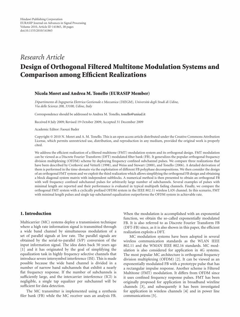
Hindawi Publishing CorporationEURASIP Journal on Advances in Signal ProcessingVolume 2010, Article ID 141865, 18 pagesdoi:10.1155/2010/141865
Research Article
Design of Orthogonal Filtered Multitone Modulation Systems andComparison among Efficient Realizations
Nicola Moret and Andrea M. Tonello (EURASIP Member)
Dipartimento di Ingegneria Elettrica Gestionale e Meccanica (DIEGM), Universita degli Studi di Udine,Via delle Scienze 208, 33100, Udine, Italy
Correspondence should be addressed to Andrea M. Tonello, [email protected]
Received 8 July 2009; Revised 19 October 2009; Accepted 31 December 2009
Academic Editor: Faouzi Bader
Copyright © 2010 N. Moret and A. M. Tonello. This is an open access article distributed under the Creative Commons AttributionLicense, which permits unrestricted use, distribution, and reproduction in any medium, provided the original work is properlycited.
We address the efficient realization of a filtered multitone (FMT) modulation system and its orthogonal design. FMT modulationcan be viewed as a Discrete Fourier Transform (DFT) modulated filter bank (FB). It generalizes the popular orthogonal frequencydivision multiplexing (OFDM) scheme by deploying frequency confined subchannel pulses. We compare three realizations thathave been described by Cvetkovic and Vetterli (1998), and Weiss and Stewart (2000), and Tonello (2006). A detailed derivation ofthem is performed in the time-domain via the exploitation of different FB polyphase decompositions. We then consider the designof an orthogonal FMT system and we exploit the third realization which allows simplifying the orthogonal FB design and obtaininga block diagonal system matrix with independent subblocks. A numerical method is then presented to obtain an orthogonal FBwith well frequency confined subchannel pulses for arbitrarily large number of subchannels. Several examples of pulses withminimal length are reported and their performance is evaluated in typical multipath fading channels. Finally, we compare theorthogonal FMT system with a cyclically prefixed OFDM system in the IEEE 802.11 wireless LAN channel. In this scenario, FMTwith minimal length pulses and single tap subchannel equalization outperforms the OFDM system in achievable rate.
1. Introduction
Multicarrier (MC) systems deploy a transmission techniquewhere a high rate information signal is transmitted througha wide band channel by simultaneous modulation of aset of parallel signals at low rate. The parallel signals areobtained by the serial-to-parallel (S/P) conversion of theinput information signal. The idea dates back 50 years ago[1] and it has originated by the goal of simplifying theequalization task in highly frequency selective channels thatintroduce severe intersymbol interference (ISI). This is madepossible because the wide band channel is divided in anumber of narrow band subchannels that exhibit a nearlyflat frequency response. If the number of subchannels issufficiently large, and the intercarrier interference (ICI) isnegligible, a single tap equalizer per subchannel will besufficient for data detection.
The MC transmitter is implemented using a synthesisfiler bank (FB) while the MC receiver uses an analysis FB.
When the modulation is accomplished with an exponentialfunction, we obtain the so-called exponentially modulatedFB. It is also referred to as Discrete Fourier Transform FB(DFT-FB) since, as it is also shown in this paper, the efficientrealization exploits a DFT.
MC modulation systems have been adopted in severalwireless communication standards as the WLAN IEEE802.11 and the WMAN IEEE 802.16 standards. MC mod-ulation is also considered for application in 4G systems.The most popular MC architecture is orthogonal frequencydivision multiplexing (OFDM) [2]. It can be viewed as anexponentially modulated FB with a prototype pulse that hasa rectangular impulse response. Another scheme is FilteredMultitone (FMT) modulation. It differs from OFDM sinceit uses confined frequency response pulses. FMT has beenoriginally proposed for application in broadband wirelinechannels [3], and subsequently it has been investigatedfor application in wireless channels [4] and in power linecommunications [5].
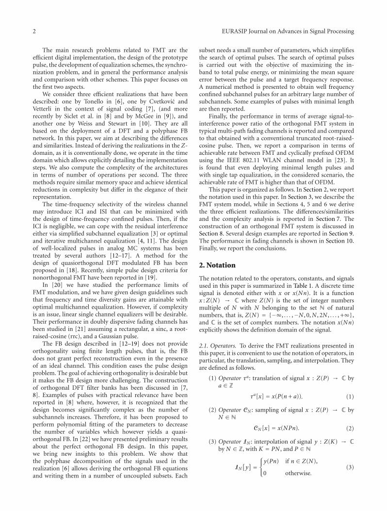
2 EURASIP Journal on Advances in Signal Processing
The main research problems related to FMT are theefficient digital implementation, the design of the prototypepulse, the development of equalization schemes, the synchro-nization problem, and in general the performance analysisand comparison with other schemes. This paper focuses onthe first two aspects.
We consider three efficient realizations that have beendescribed: one by Tonello in [6], one by Cvetkovic andVetterli in the context of signal coding [7], (and morerecently by Siclet et al. in [8] and by McGee in [9]), andanother one by Weiss and Stewart in [10]. They are allbased on the deployment of a DFT and a polyphase FBnetwork. In this paper, we aim at describing the differencesand similarities. Instead of deriving the realizations in the Z-domain, as it is conventionally done, we operate in the timedomain which allows explicitly detailing the implementationsteps. We also compute the complexity of the architecturesin terms of number of operations per second. The threemethods require similar memory space and achieve identicalreductions in complexity but differ in the elegance of theirrepresentation.
The time-frequency selectivity of the wireless channelmay introduce ICI and ISI that can be minimized withthe design of time-frequency confined pulses. Then, if theICI is negligible, we can cope with the residual interferenceeither via simplified subchannel equalization [3] or optimaland iterative multichannel equalization [4, 11]. The designof well-localized pulses in analog MC systems has beentreated by several authors [12–17]. A method for thedesign of quasiorthogonal DFT modulated FB has beenproposed in [18]. Recently, simple pulse design criteria fornonorthogonal FMT have been reported in [19].
In [20] we have studied the performance limits ofFMT modulation, and we have given design guidelines suchthat frequency and time diversity gains are attainable withoptimal multichannel equalization. However, if complexityis an issue, linear single channel equalizers will be desirable.Their performance in doubly dispersive fading channels hasbeen studied in [21] assuming a rectangular, a sinc, a root-raised-cosine (rrc), and a Gaussian pulse.
The FB design described in [12–19] does not provideorthogonality using finite length pulses, that is, the FBdoes not grant perfect reconstruction even in the presenceof an ideal channel. This condition eases the pulse designproblem. The goal of achieving orthogonality is desirable butit makes the FB design more challenging. The constructionof orthogonal DFT filter banks has been discussed in [7,8]. Examples of pulses with practical relevance have beenreported in [8] where, however, it is recognized that thedesign becomes significantly complex as the number ofsubchannels increases. Therefore, it has been proposed toperform polynomial fitting of the parameters to decreasethe number of variables which however yields a quasi-orthogonal FB. In [22] we have presented preliminary resultsabout the perfect orthogonal FB design. In this paper,we bring new insights to this problem. We show thatthe polyphase decomposition of the signals used in therealization [6] allows deriving the orthogonal FB equationsand writing them in a number of uncoupled subsets. Each
subset needs a small number of parameters, which simplifiesthe search of optimal pulses. The search of optimal pulsesis carried out with the objective of maximizing the in-band to total pulse energy, or minimizing the mean squareerror between the pulse and a target frequency response.A numerical method is presented to obtain well frequencyconfined subchannel pulses for an arbitrary large number ofsubchannels. Some examples of pulses with minimal lengthare then reported.
Finally, the performance in terms of average signal-to-interference power ratio of the orthogonal FMT system intypical multi-path fading channels is reported and comparedto that obtained with a conventional truncated root-raised-cosine pulse. Then, we report a comparison in terms ofachievable rate between FMT and cyclically prefixed OFDMusing the IEEE 802.11 WLAN channel model in [23]. Itis found that even deploying minimal length pulses andwith single tap equalization, in the considered scenario, theachievable rate of FMT is higher than that of OFDM.
This paper is organized as follows. In Section 2, we reportthe notation used in this paper. In Section 3, we describe theFMT system model, while in Sections 4, 5 and 6 we derivethe three efficient realizations. The differences/similaritiesand the complexity analysis is reported in Section 7. Theconstruction of an orthogonal FMT system is discussed inSection 8. Several design examples are reported in Section 9.The performance in fading channels is shown in Section 10.Finally, we report the conclusions.
2. Notation
The notation related to the operators, constants, and signalsused in this paper is summarized in Table 1. A discrete timesignal is denoted either with x or x(Nn). It is a functionx :Z(N) → C where Z(N) is the set of integer numbersmultiple of N with N belonging to the set N of naturalnumbers, that is, Z(N) = {−∞, . . . ,−N , 0,N , 2N , . . . , +∞},and C is the set of complex numbers. The notation x(Nn)explicitly shows the definition domain of the signal.
2.1. Operators. To derive the FMT realizations presented inthis paper, it is convenient to use the notation of operators, inparticular, the translation, sampling, and interpolation. Theyare defined as follows.
(1) Operator τa: translation of signal x : Z(P) → C bya ∈ Z
τa[x] = x(P(n + a)). (1)
(2) Operator CN : sampling of signal x : Z(P) → C byN ∈ N
CN [x] = x(NPn). (2)
(3) Operator IN : interpolation of signal y : Z(K) → Cby N ∈ Z, with K = PN , and P ∈ N
IN[y] =
⎧⎨⎩y(Pn) if n ∈ Z(N),
0 otherwise.(3)
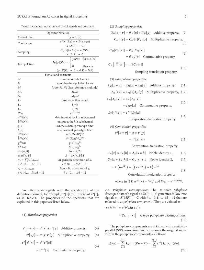
EURASIP Journal on Advances in Signal Processing 3
Table 1: Operator notation and useful signals and constants.
Operator Notation
Convolution [x ∗ h](n)
Translationτa[x](Pn) = x(P(n + a))
(x : Z(P) → C)
SamplingCN [x](NPn) = x(NPn)
(x : Z(P) → C)
InterpolationIN [y](Pn) =
⎧⎪⎨⎪⎩
y(Pn) if n ∈ Z(N)
0 otherwise
(y : Z(K) → C and K = NP)
Signals and constants
M number of subchannels
N sampling-interpolation factor
M1 l.c.m.(M,N) (least common multiple)
M0 M1/N
N0 M1/M
Lf prototype filter length
LM Lf /N
LN L f /M
WM e− j(2π/M)
a(k)(Nn) data input at the kth subchannel
b(k)(Nn) output at the kth subchannel
g(n) synthesis bank prototype filter
h(n) analysis bank prototype filter
a(k)(Nn) a(k)(Nn)WkNnM
b(k)(Nn) b(k)(Nn)W−kNnM
g(k)(n) g(n)W−knM
h(k)(n) h(n)W−knM
div[A,B] floor(A/B)
mod[A,B] A− div[A,B] B
ya =∑N0−1
b=0 xa+Mb M-periodic repetition of xia ∈ {0, . . . ,M − 1} i ∈ {0, . . . ,N0M − 1}xa = ymod[a,M] N0-cyclic extension of yia ∈ {0, . . . ,N0M − 1} i ∈ {0, . . . ,M − 1}
We often write signals with the specification of thedefinition domain, for example, τa[x](Pn) instead of τa[x],as in Table 1. The properties of the operators that areexploited in this paper are listed below.
(1) Translation properties:
τa[x + y
] = τa[x] + τa[y]
Additive property, (4)
τa[xy] = τa[x]τa
[y]
Multiplicative property, (5)
τa[τb[x]
]= τb[τa[x]]
= τa+b[x] Commutative property.(6)
(2) Sampling properties:
CM[x + y
] = CM[x] + CM[y]
Additive property, (7)
CM[xy] = CM[x]CM
[y]
Multiplicative property,(8)
CM[CN [x]] = CN [CM[x]]
= CMN [x] Commutative property,(9)
CN
[τNa[x]
]= τa[CN [x]]
Sampling-translation property.(10)
(3) Interpolation properties:
IM[x + y
] = IM[x] + IM[y]
Additive property, (11)
IM[xy] = IM[x]IM
[y]
Multiplicative property, (12)
IM[IN [x]] = IN [IM[x]]
= IMN [x] Commutative property,(13)
IN [τa[x]] = τNa[IN [x]]
Interpolation-translation property.(14)
(4) Convolution properties:
τa[x ∗ y
] = x ∗ τa[y]
= τa[x]∗ y
Convolution-translation property,
(15)
IN [x]∗ IN [h] = IN [x ∗ h] Noble identity 1, (16)
CN [x ∗ IN [h]] = CN [x]∗ h Noble identity 2, (17)
x ∗(hw(k)
)=((xw(−k)
)∗ h)w(k)
Convolution-modulation property,(18)
where in (18) w(k)(n) =WknM and WM = e− j(2π/M).
2.2. Polyphase Decomposition. The M-order polyphasedecomposition of a signal x : Z(P) → C generates M low-ratesignals xi : Z(MP) → C with i ∈ {0, 1, . . . ,M − 1} that arereferred to as polyphase components. They are defined as
xi(MPn) = x(P(Mn + i))
= CM
[τi[x]
]A-type polyphase decomposition.
(19)
The polyphase components are obtained with a serial-to-parallel (S/P) conversion. We can recover the original signalx from the polyphase components as follows:
x(Pn) =M−1∑
i=0
IM[xi](Pn− Pi) =M−1∑
i=0
τ−i[IM[xi]](Pn).
(20)
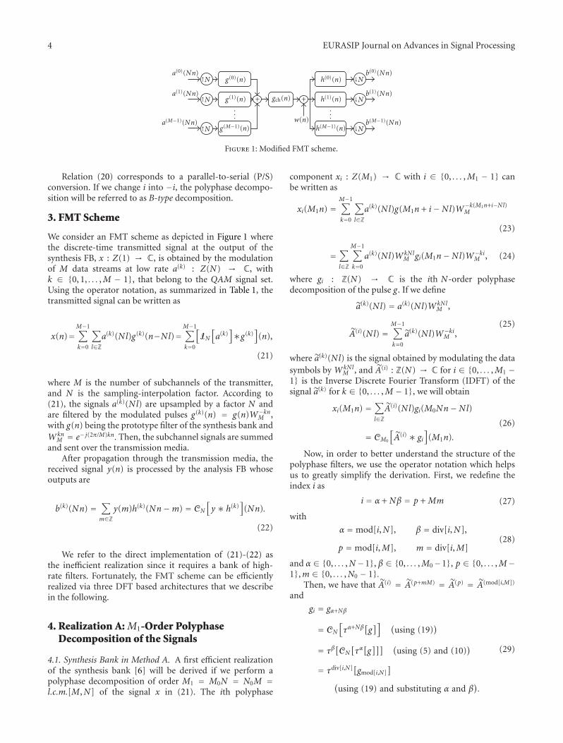
4 EURASIP Journal on Advances in Signal Processing
a(M−1)(Nn)
a(1)(Nn)
a(0)(Nn)
↑N
↑N
↑N
↓N
↓N
↓N
g(M−1)(n)
g(1)(n)
g(0)(n)
++ gch(n)
b(M−1)(Nn)
b(1)(Nn)
b(0)(Nn)
......w(n)
h(M−1)(n)
h(1)(n)
h(0)(n)
Figure 1: Modified FMT scheme.
Relation (20) corresponds to a parallel-to-serial (P/S)conversion. If we change i into −i, the polyphase decompo-sition will be referred to as B-type decomposition.
3. FMT Scheme
We consider an FMT scheme as depicted in Figure 1 wherethe discrete-time transmitted signal at the output of thesynthesis FB, x : Z(1) → C, is obtained by the modulationof M data streams at low rate a(k) : Z(N) → C, withk ∈ {0, 1, . . . ,M − 1}, that belong to the QAM signal set.Using the operator notation, as summarized in Table 1, thetransmitted signal can be written as
x(n)=M−1∑
k=0
∑
l∈Za(k)(Nl)g(k)(n−Nl)=
M−1∑
k=0
[IN[a(k)]∗g(k)
](n),
(21)
where M is the number of subchannels of the transmitter,and N is the sampling-interpolation factor. According to(21), the signals a(k)(Nl) are upsampled by a factor N andare filtered by the modulated pulses g(k)(n) = g(n)W−kn
M ,with g(n) being the prototype filter of the synthesis bank andWkn
M = e− j(2π/M)kn. Then, the subchannel signals are summedand sent over the transmission media.
After propagation through the transmission media, thereceived signal y(n) is processed by the analysis FB whoseoutputs are
b(k)(Nn) =∑
m∈Zy(m)h(k)(Nn−m) = CN
[y ∗ h(k)
](Nn).
(22)
We refer to the direct implementation of (21)-(22) asthe inefficient realization since it requires a bank of high-rate filters. Fortunately, the FMT scheme can be efficientlyrealized via three DFT based architectures that we describein the following.
4. Realization A: M1-Order PolyphaseDecomposition of the Signals
4.1. Synthesis Bank in Method A. A first efficient realizationof the synthesis bank [6] will be derived if we perform apolyphase decomposition of order M1 = M0N = N0M =l.c.m.[M,N] of the signal x in (21). The ith polyphase
component xi : Z(M1) → C with i ∈ {0, . . . ,M1 − 1} canbe written as
xi(M1n) =M−1∑
k=0
∑
l∈Za(k)(Nl)g(M1n + i−Nl)W−k(M1n+i−Nl)
M
(23)
=∑
l∈Z
M−1∑
k=0
a(k)(Nl)WkNlM gi(M1n−Nl)W−ki
M , (24)
where gi : Z(N) → C is the ith N-order polyphasedecomposition of the pulse g. If we define
a(k)(Nl) = a(k)(Nl)WkNlM ,
A(i)(Nl) =M−1∑
k=0
a(k)(Nl)W−kiM ,
(25)
where a(k)(Nl) is the signal obtained by modulating the datasymbols by WkNl
M , and A(i) : Z(N) → C for i ∈ {0, . . . ,M1 −1} is the Inverse Discrete Fourier Transform (IDFT) of thesignal a(k) for k ∈ {0, . . . ,M − 1}, we will obtain
xi(M1n) =∑
l∈ZA(i)(Nl)gi(M0Nn−Nl)
= CM0
[A(i) ∗ gi
](M1n).
(26)
Now, in order to better understand the structure of thepolyphase filters, we use the operator notation which helpsus to greatly simplify the derivation. First, we redefine theindex i as
i = α +Nβ = p +Mm (27)
with
α = mod[i,N], β = div[i,N],
p = mod[i,M], m = div[i,M](28)
and α ∈ {0, . . . ,N−1}, β ∈ {0, . . . ,M0−1}, p ∈ {0, . . . ,M−1},m ∈ {0, . . . ,N0 − 1}.
Then, we have that A(i) = A(p+mM) = A(p) = A(mod[i,M])
and
gi = gα+Nβ
= CN
[τα+Nβ[g
]] (using (19)
)
= τβ[CN[τα[g]]] (
using (5) and (10))
= τdiv[i,N][gmod[i,N]]
(using (19) and substituting α and β
).
(29)
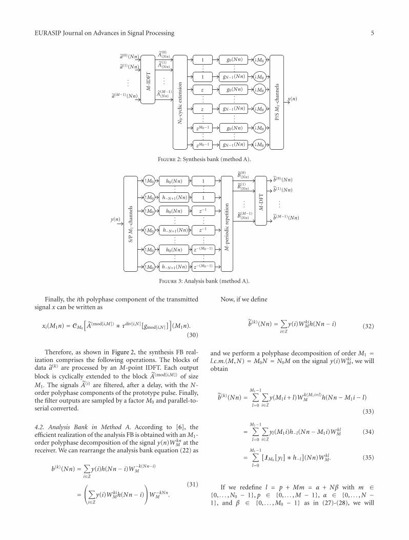
EURASIP Journal on Advances in Signal Processing 5
a(0)(Nn)
a(1)(Nn)
a(M−1)(Nn)
...
M-I
DFT
A(0)(Nn)
A(1)(Nn)
A(M−1)(Nn)
...
N0-c
yclic
exte
nsi
on
1...1
z...
z...
zM0−1
...
zM0−1 gN−1(Nn)
g0(Nn)
gN−1(Nn)
g0(Nn)
gN−1(Nn)
g0(Nn)
↓M0
↓M0
↓M0
↓M0
↓M0
↓M0
x(n)
P/SM
1-c
han
nel
s
...
...
...
...
Figure 2: Synthesis bank (method A).
y(n)
S/PM
1-c
han
nel
s
↑M0
↑M0
↑M0
↑M0
↑M0
↑M0
h0(Nn)
h−N+1(Nn)
h0(Nn)
h−N+1(Nn)
h0(Nn)
h−N+1(Nn)
1
1
z−1
z−1
z−(M0−1)
z−(M0−1)
M-p
erio
dic
repe
titi
on
B(0)(Nn)
B(1)(Nn)
B(M−1)(Nn)
M-D
FT
b(0)(Nn)
b(1)(Nn)
b(M−1)(Nn)
...
...
...
...
...
...
...
...
......
Figure 3: Analysis bank (method A).
Finally, the ith polyphase component of the transmittedsignal x can be written as
xi(M1n) = CM0
[A(mod[i,M]) ∗ τdiv[i,N][gmod[i,N]
]](M1n).
(30)
Therefore, as shown in Figure 2, the synthesis FB real-ization comprises the following operations. The blocks ofdata a(k) are processed by an M-point IDFT. Each outputblock is cyclically extended to the block A(mod[i,M]) of sizeM1. The signals A(i) are filtered, after a delay, with the N-order polyphase components of the prototype pulse. Finally,the filter outputs are sampled by a factor M0 and parallel-to-serial converted.
4.2. Analysis Bank in Method A. According to [6], theefficient realization of the analysis FB is obtained with anM1-order polyphase decomposition of the signal y(n)Wkn
M at thereceiver. We can rearrange the analysis bank equation (22) as
b(k)(Nn) =∑
i∈Zy(i)h(Nn− i)W−k(Nn−i)
M
=⎛⎝∑
i∈Zy(i)Wki
Mh(Nn− i)⎞⎠W−kNn
M .
(31)
Now, if we define
b(k)(Nn) =∑
i∈Zy(i)Wki
Mh(Nn− i) (32)
and we perform a polyphase decomposition of order M1 =l.c.m.(M,N) = M0N = N0M on the signal y(i)Wki
M , we willobtain
b(k)(Nn) =M1−1∑
l=0
∑
i∈Zy(M1i + l)Wk(M1i+l)
M h(Nn−M1i− l)
(33)
=M1−1∑
l=0
∑
i∈Zyl(M1i)h−l(Nn−M1i)Wkl
M (34)
=M1−1∑
l=0
[IM0
[yl]∗ h−l
](Nn)Wkl
M. (35)
If we redefine l = p + Mm = α + Nβ with m ∈{0, . . . ,N0 − 1}, p ∈ {0, . . . ,M − 1}, α ∈ {0, . . . ,N −1}, and β ∈ {0, . . . ,M0 − 1} as in (27)-(28), we will
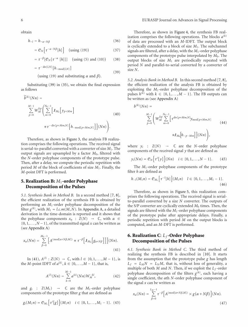
6 EURASIP Journal on Advances in Signal Processing
obtain
h−l = h−α−Nβ (36)
= CN
[τ−α−Nβ[h]
] (using (19)
)(37)
= τ−β[CN [τ−α [h]]](using (5) and (10)
)(38)
= τ−div[l,N][h−mod[l,N]]
(using (19) and substituting α and β
).
(39)
Substituting (39) in (35), we obtain the final expressionas follows
b(k)(Nn) =M−1∑
p=0
WkpM
⎛⎝N0−1∑
m=0
[IM0
[yp+Mm
]
∗τ−div[p+Mm,N][h−mod[p+Mm,N]
]](Nn)
⎞⎠.
(40)
Therefore, as shown in Figure 3, the analysis FB realiza-tion comprises the following operations. The received signalis serial-to-parallel converted with a converter of sizeM1. Theoutput signals are upsampled by a factor M0, filtered withthe N-order polyphase components of the prototype pulse.Then, after a delay, we compute the periodic repetition withperiod M of the block of coefficients of size M1. Finally, theM-point DFT is performed.
5. Realization B: M1-order PolyphaseDecomposition of the Pulses
5.1. Synthesis Bank in Method B. In a second method [7, 8],the efficient realization of the synthesis FB is obtained byperforming an M1-order polyphase decomposition of thefilter g(k), with M1 = l.c.m(M,N). In Appendix A, a detailedderivation in the time-domain is reported and it shows thatthe polyphase components xα : Z(N) → C, with α ∈{0, 1, . . . ,N−1}, of the transmitted signal x can be written as(see Appendix A)
xα(Nn) =M0−1∑
β=0
[A(mod[α+Nβ,M]) ∗ τ−β
[IM0
[gα+Nβ
]]](Nn).
(41)
In (41), A(l) : Z(N) → C, with l ∈ {0, 1, . . . ,M − 1}, isthe M-point IDFT of a(k), k ∈ {0, . . . ,M − 1}, that is,
A(l)(Nn) =M−1∑
k=0
a(k)(Nn)W−klM , (42)
and gi : Z(M1) → C are the M1-order polyphasecomponents of the prototype filter g that are defined as
gi(M1n) = CM1
[τi[g]]
(M1n) i ∈ {0, 1, . . . ,M1 − 1}. (43)
Therefore, as shown in Figure 4, the synthesis FB real-ization comprises the following operations. The blocks a(k)
of data are processed with an M-IDFT. The output blockis cyclically extended to a block of size M1. The subchannelsignals are filtered, after a delay, with theM1-order polyphasecomponents of the prototype pulse interpolated by M0. Theoutput blocks of size M1 are periodically repeated withperiod N and parallel-to-serial converted by a converter ofsize N .
5.2. Analysis Bank in Method B. In this second method [7, 8],the efficient realization of the analysis FB is obtained byexploiting the M1-order polyphase decomposition of thepulses h(k) with k ∈ {0, 1, . . . ,M − 1}. The FB outputs canbe written as (see Appendix A)
b(k)(Nn) =M−1∑
p=0
⎛⎝Wkp
M
N0−1∑
m=0
[τdiv[p+Mm,N]ymod[p+Mm,N]
∗IM0
[h−p−Mm
]](Nn)
⎞⎠,
(44)
where yi : Z(N) → C are the N-order polyphasecomponents of the received signal y that are defined as
yi(Nn) = CN
[τi[y]]
(Nn) i ∈ {0, 1, . . . ,N − 1}. (45)
The M1-order polyphase components of the prototypefilter h are defined as
h−l(M1n) = CM1
[τ−l[h]
](M1n) l ∈ {0, 1, . . . ,M1 − 1}.
(46)
Therefore, as shown in Figure 5, this realization com-prises the following operations. The received signal is serial-to-parallel converted by a size N converter. The outputs ofthe S/P converter are cyclically extended M0 times. Then, thesignals are filtered with the M1-order polyphase componentsof the prototype pulse after appropriate delays. Finally, aperiodic repetition with period M on the output blocks iscomputed, and an M-DFT is performed.
6. Realization C: Lf -Order PolyphaseDecomposition of the Pulses
6.1. Synthesis Bank in Method C. The third method ofrealizing the synthesis FB is described in [10]. It startsfrom the assumption that the prototype pulse g has lengthL f = LMN = LNM, that is, without loss of generality, amultiple of both M and N . Then, if we exploit the L f -orderpolyphase decomposition of the filters g(k), each having asingle coefficient, the αth N-order polyphase component ofthe signal x can be written as
xα(Nn) =LM−1∑
β=0
τ−β[A(mod[α+Nβ,M]) × g(α +Nβ
)](Nn).
(47)
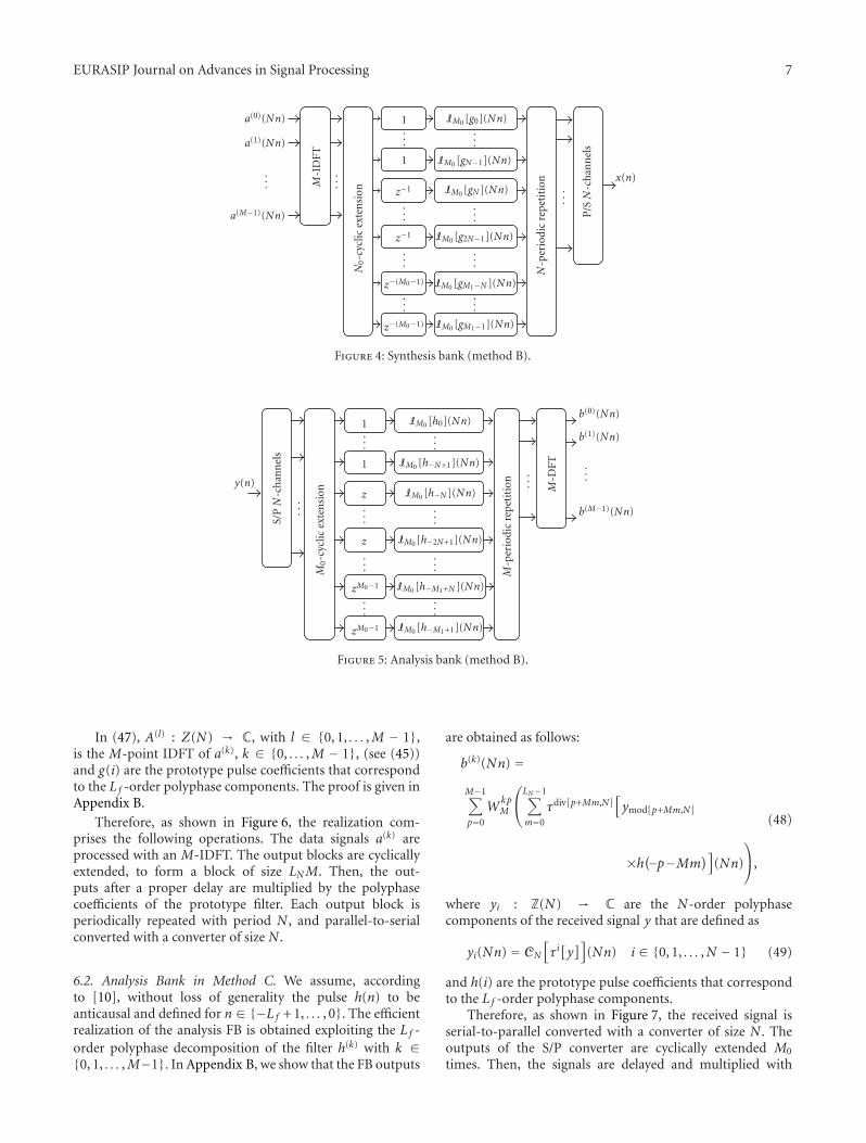
EURASIP Journal on Advances in Signal Processing 7
a(0)(Nn)
a(1)(Nn)
a(M−1)(Nn)
M-I
DFT
N0-c
yclic
exte
nsi
on
1
1
z−1
z−1
z−(M0−1)
z−(M0−1)
IM0 [g0](Nn)
IM0 [gN−1](Nn)
IM0 [gN ](Nn)
IM0 [g2N−1](Nn)
IM0 [gM1−N ](Nn)
IM0 [gM1−1](Nn)
N-p
erio
dic
repe
titi
on
P/SN
-ch
ann
els
......
...
...
...
...
...
...
...
...
...
x(n)
Figure 4: Synthesis bank (method B).
b(0)(Nn)
b(1)(Nn)
b(M−1)(Nn)
M-D
FT
M0-c
yclic
exte
nsi
on
1
1
z
z
zM0−1
zM0−1
IM0 [h0](Nn)
IM0 [h−N+1](Nn)
IM0 [h−N ](Nn)
IM0 [h−2N+1](Nn)
IM0 [h−M1+N ](Nn)
IM0 [h−M1+1](Nn)
M-p
erio
dic
repe
titi
on
S/PN
-ch
ann
els
...
...
...
...
...
...
...
...
...
...
...y(n)
Figure 5: Analysis bank (method B).
In (47), A(l) : Z(N) → C, with l ∈ {0, 1, . . . ,M − 1},is the M-point IDFT of a(k), k ∈ {0, . . . ,M − 1}, (see (45))and g(i) are the prototype pulse coefficients that correspondto the L f -order polyphase components. The proof is given inAppendix B.
Therefore, as shown in Figure 6, the realization com-prises the following operations. The data signals a(k) areprocessed with an M-IDFT. The output blocks are cyclicallyextended, to form a block of size LNM. Then, the out-puts after a proper delay are multiplied by the polyphasecoefficients of the prototype filter. Each output block isperiodically repeated with period N , and parallel-to-serialconverted with a converter of size N .
6.2. Analysis Bank in Method C. We assume, accordingto [10], without loss of generality the pulse h(n) to beanticausal and defined for n ∈ {−L f + 1, . . . , 0}. The efficientrealization of the analysis FB is obtained exploiting the L f -order polyphase decomposition of the filter h(k) with k ∈{0, 1, . . . ,M−1}. In Appendix B, we show that the FB outputs
are obtained as follows:
b(k)(Nn) =M−1∑
p=0
WkpM
⎛⎝LN−1∑
m=0
τdiv[p+Mm,N][ymod[p+Mm,N]
×h(−p−Mm)]
(Nn)
⎞⎠,
(48)
where yi : Z(N) → C are the N-order polyphasecomponents of the received signal y that are defined as
yi(Nn) = CN
[τi[y]]
(Nn) i ∈ {0, 1, . . . ,N − 1} (49)
and h(i) are the prototype pulse coefficients that correspondto the L f -order polyphase components.
Therefore, as shown in Figure 7, the received signal isserial-to-parallel converted with a converter of size N . Theoutputs of the S/P converter are cyclically extended M0
times. Then, the signals are delayed and multiplied with
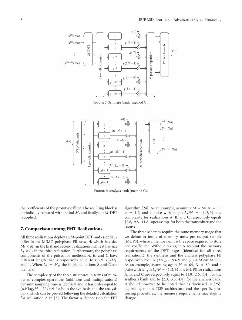
8 EURASIP Journal on Advances in Signal Processing
a(0)(Nn)
a(1)(Nn)
a(M−1)(Nn)
M-I
DFT
LN
-cyc
licex
ten
sion
1
1
z−1
z−1
z−(LM−1)
z−(LM−1)
g(0)
g(N − 1)
g(N)
g(2N − 1)
g(L f −N)
g(L f − 1)
N-p
erio
dic
repe
titi
on
P/SN
-ch
ann
els
......
...
...
...
...
...
x(n)
×
×
×
×
×
×
Figure 6: Synthesis bank (method C).
b(0)(Nn)
b(1)(Nn)
b(M−1)(Nn)
M-D
FT
LM
-cyc
licex
ten
sion
1
1
z
z
zLM−1
zLM−1
h(0)
h(−N + 1)
h(−N)
h(−2N + 1)
h(−L f +N)
h(−L f + 1)
M-p
erio
dic
repe
titi
on
S/PN
-ch
ann
els
.........
...
...
...
...
y(n)
×
×
×
×
×
×
Figure 7: Analysis bank (method C).
the coefficients of the prototype filter. The resulting block isperiodically repeated with period M, and finally, an M-DFTis applied.
7. Comparison among FMT Realizations
All three realizations deploy an M-point DFT, and essentiallydiffer in the MIMO polyphase FB network which has sizeM1 ×M1 in the first and second realizations, while it has sizeL f × L f in the third realization. Furthermore, the polyphasecomponents of the pulses for methods A, B, and C havedifferent length that is respectively equal to L f /N , L f /M1,and 1. When L f = M1, the implementations B and C areidentical.
The complexity of the three structures in terms of num-ber of complex operations (additions and multiplications)per unit sampling time is identical and it has order equal to(αMlog2M + 2L f )/N for both the synthesis and the analysisbank which can be proved following the detailed calculationfor realization A in [5]. The factor α depends on the FFT
algorithm [24]. As an example, assuming M = 64, N = 80,α = 1.2, and a pulse with length L f /N = {1, 2, 3}, thecomplexity for realizations A, B, and C respectively equals{7.8, 9.8, 11.8} oper./samp. for both the transmitter and thereceiver.
The three schemes require the same memory usage thatwe define in terms of memory units per output sample(MUPS), where a memory unit is the space required to storeone coefficient. Without taking into account the memoryrequirements of the DFT stages (identical for all threerealizations), the synthesis and the analysis polyphase FBrespectively require (MLM + N)/N and (L f + M)/M MUPS.As an example, assuming again M = 64, N = 80, and apulse with length L f /N = {1, 2, 3}, the MUPS for realizationsA, B, and C are respectively equal to {1.8, 2.6, 3.4} for thesynthesis bank and to {2.3, 3.5, 4.8} for the analysis bank.It should however to be noted that as discussed in [25],depending on the DSP architecture and the specific pro-cessing procedures, the memory requirements may slightlychange.
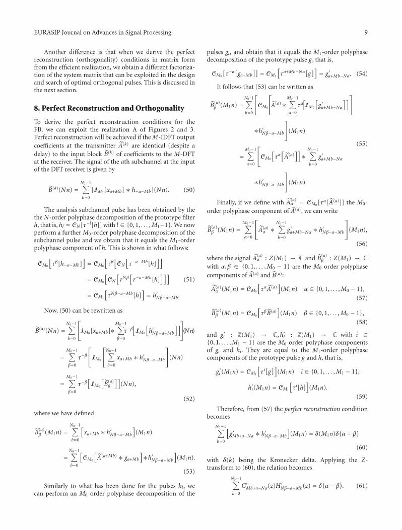
EURASIP Journal on Advances in Signal Processing 9
Another difference is that when we derive the perfectreconstruction (orthogonality) conditions in matrix formfrom the efficient realization, we obtain a different factoriza-tion of the system matrix that can be exploited in the designand search of optimal orthogonal pulses. This is discussed inthe next section.
8. Perfect Reconstruction and Orthogonality
To derive the perfect reconstruction conditions for theFB, we can exploit the realization A of Figures 2 and 3.Perfect reconstruction will be achieved if theM-IDFT outputcoefficients at the transmitter A(k) are identical (despite adelay) to the input block B(k) of coefficients to the M-DFTat the receiver. The signal of the ath subchannel at the inputof the DFT receiver is given by
B(a)(Nn) =N0−1∑
b=0
[IM0 [xa+Mb]∗ h−a−Mb
](Nn). (50)
The analysis subchannel pulse has been obtained by thethe N-order polyphase decomposition of the prototype filterh, that is, hl = CN [τ−l[h]] with l ∈ {0, 1, . . . ,M1−1}. We nowperform a further M0-order polyphase decomposition of thesubchannel pulse and we obtain that it equals the M1-orderpolyphase component of h. This is shown in what follows:
CM0
[τβ[h−a−Mb]
]= CM0
[τβ[CN
[τ−a−Mb[h]
]]
= CM0
[CN
[τNβ
[τ−a−Mb[h]
]]]
= CM1
[τNβ−a−Mb[h]
]= h′Nβ−a−Mb.
(51)
Now, (50) can be rewritten as
B(a)(Nn) =N0−1∑
b=0
⎡⎣IM0 [xa+Mb]∗
M0−1∑
β=0
τ−β[IM0
[h′Nβ−a−Mb
]]⎤⎦(Nn)
=M0−1∑
β=0
τ−β⎡⎣IM0
⎡⎣N0−1∑
b=0
xa+Mb ∗ h′Nβ−a−Mb
⎤⎦(Nn)
=M0−1∑
β=0
τ−β[IM0
[B(a)β
]](Nn),
(52)
where we have defined
B(a)β (M1n) =
N0−1∑
b=0
[xa+Mb ∗ h′Nβ−a−Mb
](M1n)
=N0−1∑
b=0
[CM0
[A(a+Mb) ∗ ga+Mb
]∗h′Nβ−a−Mb
](M1n).
(53)
Similarly to what has been done for the pulses hl, wecan perform an M0-order polyphase decomposition of the
pulses gl, and obtain that it equals the M1-order polyphasedecomposition of the prototype pulse g, that is,
CM0
[τ−α[ga+Mb
]] = CM1
[τa+Mb−Nα[g
]] = g′a+Mb−Nα. (54)
It follows that (53) can be written as
B(a)β (M1n) =
N0−1∑
b=0
⎡⎣CM0
⎡⎣A(a)∗
M0−1∑
α=0
τα[IM0
[g′a+Mb−Nα
]]⎤⎦
∗h′Nβ−a−Mb
⎤⎦(M1n)
=M0−1∑
α=0
⎡⎣CM0
[τα[A(a)
]]∗
N0−1∑
b=0
g′a+Mb−Nα
∗h′Nβ−a−Mb
⎤⎦(M1n).
(55)
Finally, if we define with A(a)α = CM0 [τα[A(a)]] the M0-
order polyphase component of A(a), we can write
B(a)β (M1n) =
M0−1∑
α=0
⎡⎣A(a)
α ∗N0−1∑
b=0
g′a+Mb−Nα ∗ h′Nβ−a−Mb
⎤⎦(M1n),
(56)
where the signal A(a)α : Z(M1) → C and B(a)
β : Z(M1) → Cwith α,β ∈ {0, 1, . . . ,M0 − 1} are the M0 order polyphasecomponents of A(a) and B(a):
A(a)α (M1n) = CM0
[ταA(a)
](M1n) α ∈ {0, 1, . . . ,M0 − 1},
(57)
B(a)β (M1n) = CM0
[τβB(a)
](M1n) β ∈ {0, 1, . . . ,M0 − 1},
(58)
and g′i : Z(M1) → C,h′i : Z(M1) → C with i ∈{0, 1, . . . ,M1 − 1} are the M0 order polyphase componentsof gi and hi. They are equal to the M1-order polyphasecomponents of the prototype pulse g and h, that is,
g′i (M1n) = CM1
[τi[g]]
(M1n) i ∈ {0, 1, . . . ,M1 − 1},
h′i (M1n) = CM1
[τi[h]
](M1n).
(59)
Therefore, from (57) the perfect reconstruction conditionbecomes
N0−1∑
b=0
[g′Mb+a−Nα ∗ h′Nβ−a−Mb
](M1n) = δ(M1n)δ
(α− β)
(60)
with δ(k) being the Kronecker delta. Applying the Z-transform to (60), the relation becomes
N0−1∑
b=0
G′Mb+a−Nα(z)H′Nβ−a−Mb(z) = δ
(α− β). (61)
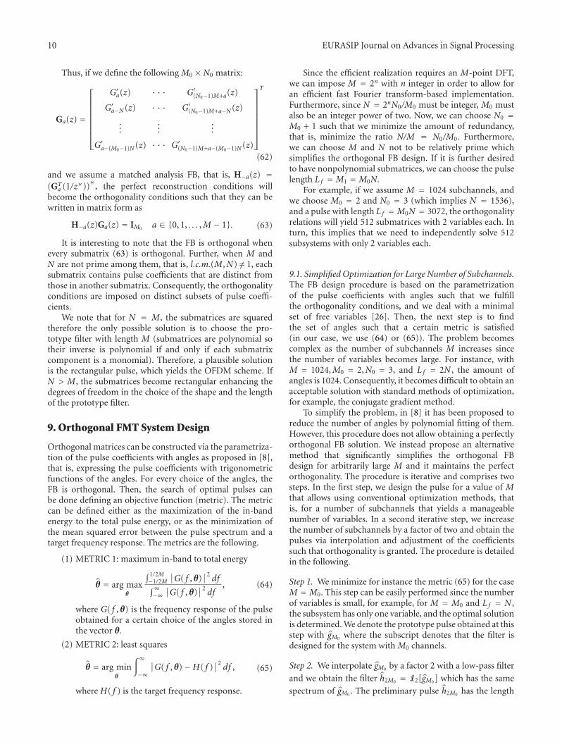
10 EURASIP Journal on Advances in Signal Processing
Thus, if we define the following M0 ×N0 matrix:
Ga(z) =
⎡⎢⎢⎢⎢⎢⎢⎢⎣
G′a(z) · · · G′(N0−1)M+a(z)
G′a−N (z) · · · G′(N0−1)M+a−N (z)
......
...
G′a−(M0−1)N (z) · · · G′(N0−1)M+a−(M0−1)N (z)
⎤⎥⎥⎥⎥⎥⎥⎥⎦
T
(62)
and we assume a matched analysis FB, that is, H−a(z) =(GT
a (1/z∗))∗
, the perfect reconstruction conditions willbecome the orthogonality conditions such that they can bewritten in matrix form as
H−a(z)Ga(z) = IM0 a ∈ {0, 1, . . . ,M − 1}. (63)
It is interesting to note that the FB is orthogonal whenevery submatrix (63) is orthogonal. Further, when M andN are not prime among them, that is, l.c.m.(M,N) /= 1, eachsubmatrix contains pulse coefficients that are distinct fromthose in another submatrix. Consequently, the orthogonalityconditions are imposed on distinct subsets of pulse coeffi-cients.
We note that for N = M, the submatrices are squaredtherefore the only possible solution is to choose the pro-totype filter with length M (submatrices are polynomial sotheir inverse is polynomial if and only if each submatrixcomponent is a monomial). Therefore, a plausible solutionis the rectangular pulse, which yields the OFDM scheme. IfN > M, the submatrices become rectangular enhancing thedegrees of freedom in the choice of the shape and the lengthof the prototype filter.
9. Orthogonal FMT System Design
Orthogonal matrices can be constructed via the parametriza-tion of the pulse coefficients with angles as proposed in [8],that is, expressing the pulse coefficients with trigonometricfunctions of the angles. For every choice of the angles, theFB is orthogonal. Then, the search of optimal pulses canbe done defining an objective function (metric). The metriccan be defined either as the maximization of the in-bandenergy to the total pulse energy, or as the minimization ofthe mean squared error between the pulse spectrum and atarget frequency response. The metrics are the following.
(1) METRIC 1: maximum in-band to total energy
θ = arg maxθ
∫ 1/2M−1/2M
∣∣G( f , θ)∣∣2df
∫∞−∞∣∣G( f , θ)
∣∣2df
, (64)
where G( f , θ) is the frequency response of the pulseobtained for a certain choice of the angles stored inthe vector θ.
(2) METRIC 2: least squares
θ = arg minθ
∫∞
−∞
∣∣G( f , θ)−H( f )∣∣2df , (65)
where H( f ) is the target frequency response.
Since the efficient realization requires an M-point DFT,we can impose M = 2n with n integer in order to allow foran efficient fast Fourier transform-based implementation.Furthermore, since N = 2nN0/M0 must be integer, M0 mustalso be an integer power of two. Now, we can choose N0 =M0 + 1 such that we minimize the amount of redundancy,that is, minimize the ratio N/M = N0/M0. Furthermore,we can choose M and N not to be relatively prime whichsimplifies the orthogonal FB design. If it is further desiredto have nonpolynomial submatrices, we can choose the pulselength L f =M1 =M0N.
For example, if we assume M = 1024 subchannels, andwe choose M0 = 2 and N0 = 3 (which implies N = 1536),and a pulse with length L f =M0N = 3072, the orthogonalityrelations will yield 512 submatrices with 2 variables each. Inturn, this implies that we need to independently solve 512subsystems with only 2 variables each.
9.1. Simplified Optimization for Large Number of Subchannels.The FB design procedure is based on the parametrizationof the pulse coefficients with angles such that we fulfillthe orthogonality conditions, and we deal with a minimalset of free variables [26]. Then, the next step is to findthe set of angles such that a certain metric is satisfied(in our case, we use (64) or (65)). The problem becomescomplex as the number of subchannels M increases sincethe number of variables becomes large. For instance, withM = 1024,M0 = 2,N0 = 3, and L f = 2N , the amount ofangles is 1024. Consequently, it becomes difficult to obtain anacceptable solution with standard methods of optimization,for example, the conjugate gradient method.
To simplify the problem, in [8] it has been proposed toreduce the number of angles by polynomial fitting of them.However, this procedure does not allow obtaining a perfectlyorthogonal FB solution. We instead propose an alternativemethod that significantly simplifies the orthogonal FBdesign for arbitrarily large M and it maintains the perfectorthogonality. The procedure is iterative and comprises twosteps. In the first step, we design the pulse for a value of Mthat allows using conventional optimization methods, thatis, for a number of subchannels that yields a manageablenumber of variables. In a second iterative step, we increasethe number of subchannels by a factor of two and obtain thepulses via interpolation and adjustment of the coefficientssuch that orthogonality is granted. The procedure is detailedin the following.
Step 1. We minimize for instance the metric (65) for the caseM =M0. This step can be easily performed since the numberof variables is small, for example, for M = M0 and L f = N ,the subsystem has only one variable, and the optimal solutionis determined. We denote the prototype pulse obtained at thisstep with gM0 where the subscript denotes that the filter isdesigned for the system with M0 channels.
Step 2. We interpolate gM0 by a factor 2 with a low-pass filter
and we obtain the filter h2M0 = I2[gM0 ] which has the same
spectrum of gM0 . The preliminary pulse h2M0 has the length
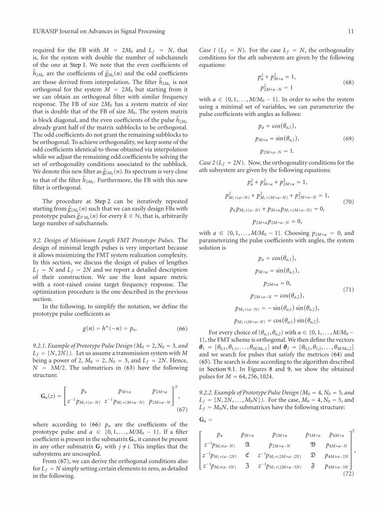
EURASIP Journal on Advances in Signal Processing 11
required for the FB with M = 2M0 and L f = N , thatis, for the system with double the number of subchannelsof the one at Step 1. We note that the even coefficients of
h2M0 are the coefficients of gM0 (n) and the odd coefficients
are those derived from interpolation. The filter h2M0 is notorthogonal for the system M = 2M0 but starting from itwe can obtain an orthogonal filter with similar frequencyresponse. The FB of size 2M0 has a system matrix of sizethat is double that of the FB of size M0. The system matrix
is block diagonal, and the even coefficients of the pulse h2M0
already grant half of the matrix subblocks to be orthogonal.The odd coefficients do not grant the remaining subblocks tobe orthogonal. To achieve orthogonality, we keep some of theodd coefficients identical to those obtained via interpolationwhile we adjust the remaining odd coefficients by solving theset of orthogonality conditions associated to the subblock.We denote this new filter as g2M0 (n). Its spectrum is very close
to that of the filter h2M0 . Furthermore, the FB with this newfilter is orthogonal.
The procedure at Step 2 can be iteratively repeatedstarting from g2M0 (n) such that we can easily design FBs withprototype pulses g2kM0 (n) for every k ∈ N, that is, arbitrarilylarge number of subchannels.
9.2. Design of Minimum Length FMT Prototype Pulses. Thedesign of minimal length pulses is very important becauseit allows minimizing the FMT system realization complexity.In this section, we discuss the design of pulses of lengthesL f = N and L f = 2N and we report a detailed descriptionof their construction. We use the least square metricwith a root-raised cosine target frequency response. Theoptimization procedure is the one described in the previoussection.
In the following, to simplify the notation, we define theprototype pulse coefficients as
g(n) = h∗(−n) = pn. (66)
9.2.1. Example of Prototype Pulse Design (M0 = 2,N0 = 3, andL f = {N , 2N}). Let us assume a transmission system withMbeing a power of 2, M0 = 2, N0 = 3, and L f = 2N . Hence,N = 3M/2. The submatrices in (63) have the followingstructure:
Ga(z) =⎡⎣
pa pM+a p2M+a
z−1pM1+(a−N) z−1pM1+(M+a−N) p2M+a−N
⎤⎦T
,
(67)
where according to (66) pn are the coefficients of theprototype pulse and a ∈ {0, 1, . . . ,M/M0 − 1}. If a filtercoefficient is present in the submatrix Gi, it cannot be presentin any other submatrix G j with j /= i. This implies that thesubsystems are uncoupled.
From (67), we can derive the orthogonal conditions alsofor L f = N simply setting certain elements to zero, as detailedin the following.
Case 1 (L f = N). For the case L f = N , the orthogonalityconditions for the ath subsystem are given by the followingequations:
p2a + p2
M+a = 1,
p22M+a−N = 1
(68)
with a ∈ {0, 1, . . . ,M/M0 − 1}. In order to solve the systemusing a minimal set of variables, we can parameterize thepulse coefficients with angles as follows:
pa = cos(θa,1),
pM+a = sin(θa,1),
p2M+a−N = 1.
(69)
Case 2 (L f = 2N). Now, the orthogonality conditions for theath subsystem are given by the following equations:
p2a + p2
M+a + p22M+a = 1,
p2M1+(a−N) + p2
M1+(M+a−N) + p22M+a−N = 1,
papM1+(a−N) + pM+a pM1+(M+a−N) = 0,
p2M+a p2M+a−N = 0,
(70)
with a ∈ {0, 1, . . . ,M/M0 − 1}. Choosing p2M+a = 0, andparameterizing the pulse coefficients with angles, the systemsolution is
pa = cos(θa,1),
pM+a = sin(θa,1),
p2M+a = 0,
p2M+a−N = cos(θa,2),
pM1+(a−N) = − sin(θa,1)
sin(θa,2),
pM1+(M+a−N) = cos(θa,1)
sin(θa,2).
(71)
For every choice of (θa,1, θa,2) with a ∈ {0, 1, . . . ,M/M0−1}, the FMT scheme is orthogonal. We then define the vectorsθ1 = [θ0,1, θ1,1, . . . , θM/M0,1] and θ2 = [θ0,2, θ1,2, . . . , θM/M0,2]and we search for pulses that satisfy the metrices (64) and(65). The search is done according to the algorithm describedin Section 9.1. In Figures 8 and 9, we show the obtainedpulses for M = 64, 256, 1024.
9.2.2. Example of Prototype Pulse Design (M0 = 4,N0 = 5, andL f = {N , 2N , . . . ,M0N}). For the case, M0 = 4, N0 = 5, andL f =M0N , the submatrices have the following structure:
Ga =⎡⎢⎢⎢⎢⎢⎢⎣
pa pM+a p2M+a p3M+a p4M+a
z−1pM1+(a−N) A p2M+a−N B p4M+a−N
z−1pM1+(a−2N) C z−1pM1+(2M+a−2N) D p4M+a−2N
z−1pM1+(a−3N) Z z−1pM1+(2M+a−3N) F p4M+a−3N
⎤⎥⎥⎥⎥⎥⎥⎦
T
,
(72)
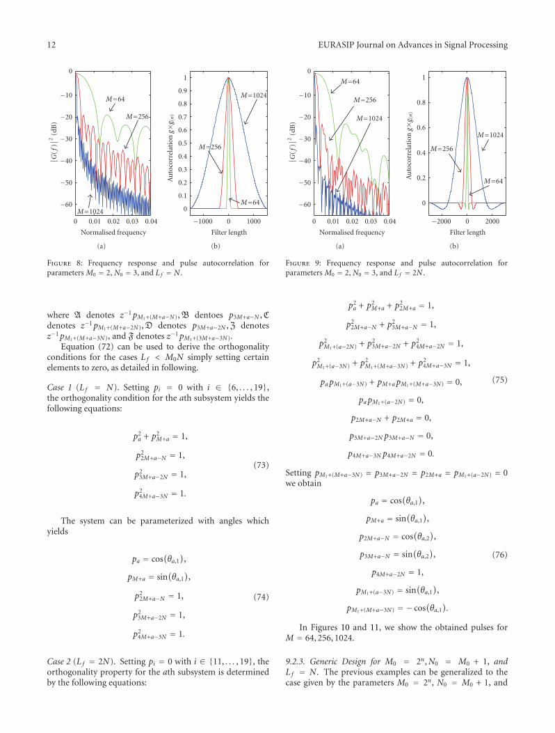
12 EURASIP Journal on Advances in Signal Processing
−60
−50
−40
−30
−20
−10
0
0 0.01 0.02 0.03 0.04
M=64
M=256
M=1024
Normalised frequency
∣ ∣ G(f
)∣ ∣2
(dB
)
(a)
0
0.1
0.2
0.3
0.4
0.5
0.6
0.7
0.8
0.9
1
−1000 0 1000
M=64
M=256
M=1024
Filter length
Au
toco
rrel
atio
ng×
g (n
)
(b)
Figure 8: Frequency response and pulse autocorrelation forparameters M0 = 2, N0 = 3, and Lf = N .
where A denotes z−1pM1+(M+a−N), B dentoes p3M+a−N , Cdenotes z−1pM1+(M+a−2N), D denotes p3M+a−2N , Z denotesz−1pM1+(M+a−3N), and F denotes z−1pM1+(3M+a−3N).
Equation (72) can be used to derive the orthogonalityconditions for the cases L f < M0N simply setting certainelements to zero, as detailed in following.
Case 1 (L f = N). Setting pi = 0 with i ∈ {6, . . . , 19},the orthogonality condition for the ath subsystem yields thefollowing equations:
p2a + p2
M+a = 1,
p22M+a−N = 1,
p23M+a−2N = 1,
p24M+a−3N = 1.
(73)
The system can be parameterized with angles whichyields
pa = cos(θa,1),
pM+a = sin(θa,1),
p22M+a−N = 1,
p23M+a−2N = 1,
p24M+a−3N = 1.
(74)
Case 2 (L f = 2N). Setting pi = 0 with i ∈ {11, . . . , 19}, theorthogonality property for the ath subsystem is determinedby the following equations:
−60
−50
−40
−30
−20
−10
0
0 0.01 0.02 0.03 0.04
M=64
M=256
M=1024
Normalised frequency
∣ ∣ G(f
)∣ ∣2
(dB
)
(a)
0
0.2
0.4
0.6
0.8
1
−2000 0 2000
M=64
M=256
M=1024
Filter length
Au
toco
rrel
atio
ng×
g (n
)
(b)
Figure 9: Frequency response and pulse autocorrelation forparameters M0 = 2, N0 = 3, and Lf = 2N .
p2a + p2
M+a + p22M+a = 1,
p22M+a−N + p2
3M+a−N = 1,
p2M1+(a−2N) + p2
3M+a−2N + p24M+a−2N = 1,
p2M1+(a−3N) + p2
M1+(M+a−3N) + p24M+a−3N = 1,
papM1+(a−3N) + pM+a pM1+(M+a−3N) = 0,
papM1+(a−2N) = 0,
p2M+a−N + p2M+a = 0,
p3M+a−2N p3M+a−N = 0,
p4M+a−3N p4M+a−2N = 0.
(75)
Setting pM1+(M+a−3N) = p3M+a−2N = p2M+a = pM1+(a−2N) = 0we obtain
pa = cos(θa,1),
pM+a = sin(θa,1),
p2M+a−N = cos(θa,2),
p3M+a−N = sin(θa,2),
p4M+a−2N = 1,
pM1+(a−3N) = sin(θa,1),
pM1+(M+a−3N) = − cos(θa,1).
(76)
In Figures 10 and 11, we show the obtained pulses forM = 64, 256, 1024.
9.2.3. Generic Design for M0 = 2n,N0 = M0 + 1, andL f = N . The previous examples can be generalized to thecase given by the parameters M0 = 2n, N0 = M0 + 1, and
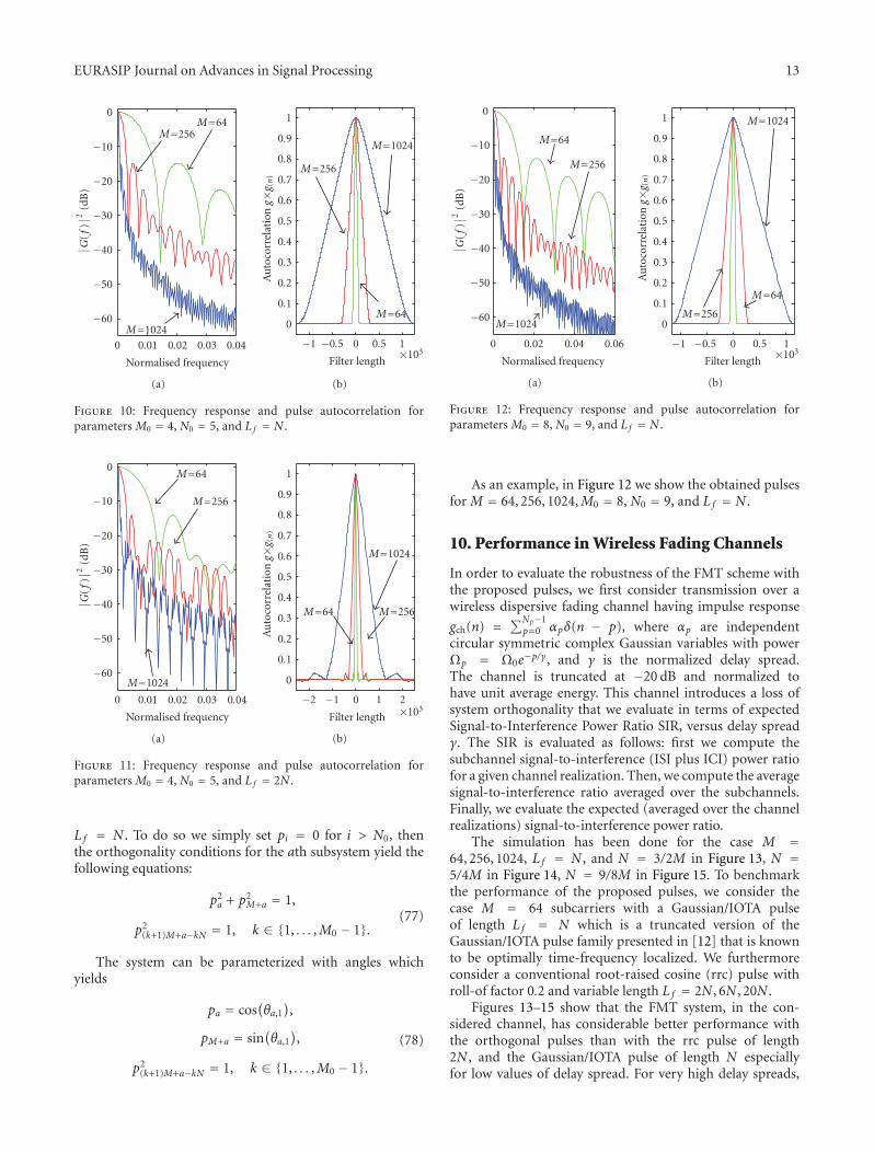
EURASIP Journal on Advances in Signal Processing 13
−60
−50
−40
−30
−20
−10
0
0 0.01 0.02 0.03 0.04
M=64M=256
M=1024
Normalised frequency
∣ ∣ G(f
)∣ ∣2
(dB
)
(a)
0
0.1
0.2
0.3
0.4
0.5
0.6
0.7
0.8
0.9
1
−1 −0.5 0 0.5 1×10³
M=64
M=256
M=1024
Filter length
Au
toco
rrel
atio
ng×
g (n
)
(b)
Figure 10: Frequency response and pulse autocorrelation forparameters M0 = 4, N0 = 5, and Lf = N .
−60
−50
−40
−30
−20
−10
0
0 0.01 0.02 0.03 0.04
M=64
M=256
M=1024
Normalised frequency
∣ ∣ G(f
)∣ ∣2
(dB
)
(a)
0
0.1
0.2
0.3
0.4
0.5
0.6
0.7
0.8
0.9
1
−2 −1 0 1 2×10³
M=64 M=256
M=1024
Filter length
Au
toco
rrel
atio
ng×
g (n
)
(b)
Figure 11: Frequency response and pulse autocorrelation forparameters M0 = 4, N0 = 5, and Lf = 2N .
L f = N . To do so we simply set pi = 0 for i > N0, thenthe orthogonality conditions for the ath subsystem yield thefollowing equations:
p2a + p2
M+a = 1,
p2(k+1)M+a−kN = 1, k ∈ {1, . . . ,M0 − 1}.
(77)
The system can be parameterized with angles whichyields
pa = cos(θa,1),
pM+a = sin(θa,1),
p2(k+1)M+a−kN = 1, k ∈ {1, . . . ,M0 − 1}.
(78)
−60
−50
−40
−30
−20
−10
0
0 0.02 0.04 0.06
M=64
M=256
M=1024
Normalised frequency
∣ ∣ G(f
)∣ ∣2
(dB
)
(a)
0
0.1
0.2
0.3
0.4
0.5
0.6
0.7
0.8
0.9
1
−1 −0.5 0 0.5 1×10³
M=64
M=256
M=1024
Filter length
Au
toco
rrel
atio
ng×
g (n
)
(b)
Figure 12: Frequency response and pulse autocorrelation forparameters M0 = 8, N0 = 9, and Lf = N .
As an example, in Figure 12 we show the obtained pulsesfor M = 64, 256, 1024,M0 = 8, N0 = 9, and L f = N .
10. Performance in Wireless Fading Channels
In order to evaluate the robustness of the FMT scheme withthe proposed pulses, we first consider transmission over awireless dispersive fading channel having impulse response
gch(n) =∑Np−1
p=0 αpδ(n − p), where αp are independentcircular symmetric complex Gaussian variables with powerΩp = Ω0e−p/γ, and γ is the normalized delay spread.The channel is truncated at −20 dB and normalized tohave unit average energy. This channel introduces a loss ofsystem orthogonality that we evaluate in terms of expectedSignal-to-Interference Power Ratio SIR, versus delay spreadγ. The SIR is evaluated as follows: first we compute thesubchannel signal-to-interference (ISI plus ICI) power ratiofor a given channel realization. Then, we compute the averagesignal-to-interference ratio averaged over the subchannels.Finally, we evaluate the expected (averaged over the channelrealizations) signal-to-interference power ratio.
The simulation has been done for the case M =64, 256, 1024, L f = N , and N = 3/2M in Figure 13, N =5/4M in Figure 14, N = 9/8M in Figure 15. To benchmarkthe performance of the proposed pulses, we consider thecase M = 64 subcarriers with a Gaussian/IOTA pulseof length L f = N which is a truncated version of theGaussian/IOTA pulse family presented in [12] that is knownto be optimally time-frequency localized. We furthermoreconsider a conventional root-raised cosine (rrc) pulse withroll-of factor 0.2 and variable length L f = 2N , 6N , 20N .
Figures 13–15 show that the FMT system, in the con-sidered channel, has considerable better performance withthe orthogonal pulses than with the rrc pulse of length2N , and the Gaussian/IOTA pulse of length N especiallyfor low values of delay spread. For very high delay spreads,
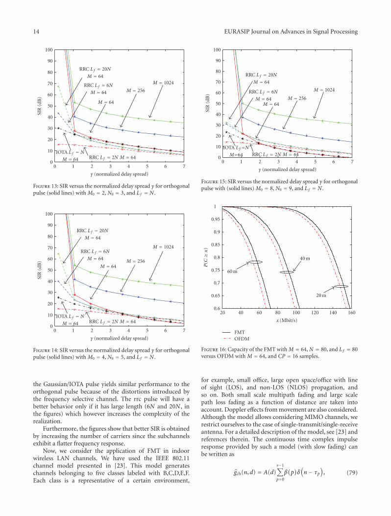
14 EURASIP Journal on Advances in Signal Processing
0 1 2 3 4 5 6 70
10
20
30
40
50
60
70
80
90
100
γ (normalized delay spread)
SIR
(dB
)
M = 256
M = 64
M = 1024
RRC L f = 20N
M = 64
RRC L f = 6N
M = 64
RRC L f = 2N M = 64IOTA L f = N
M = 64
Figure 13: SIR versus the normalized delay spread γ for orthogonalpulse (solid lines) with M0 = 2, N0 = 3, and Lf = N .
0 1 2 3 4 5 6 70
10
20
30
40
50
60
70
80
90
100
γ (normalized delay spread)
SIR
(dB
) M = 256M = 64
M = 1024
RRC L f = 20N
M = 64
RRC L f = 6N
M = 64
RRC L f = 2N M = 64IOTA L f = N
M = 64
Figure 14: SIR versus the normalized delay spread γ for orthogonalpulse (solid lines) with M0 = 4, N0 = 5, and Lf = N .
the Gaussian/IOTA pulse yields similar performance to theorthogonal pulse because of the distortions introduced bythe frequency selective channel. The rrc pulse will have abetter behavior only if it has large length (6N and 20N , inthe figures) which however increases the complexity of therealization.
Furthermore, the figures show that better SIR is obtainedby increasing the number of carriers since the subchannelsexhibit a flatter frequency response.
Now, we consider the application of FMT in indoorwireless LAN channels. We have used the IEEE 802.11channel model presented in [23]. This model generateschannels belonging to five classes labeled with B,C,D,E,F.Each class is a representative of a certain environment,
0 1 2 3 4 5 6 70
10
20
30
40
50
60
70
80
90
100
γ (normalized delay spread)
SIR
(dB
)
M = 256M = 64
M = 1024
RRC L f = 20N
M = 64
RRC L f = 6N
M = 64
RRC L f = 2N M = 64IOTA L f=N
M=64
Figure 15: SIR versus the normalized delay spread γ for orthogonalpulse with (solid lines) M0 = 8, N0 = 9, and Lf = N .
20 40 60 80 100 120 140 1600.6
0.65
0.7
0.75
0.8
0.85
0.9
0.95
1
60 m
20 m
40 m
FMTOFDM
P(C≥x)
x (Mbit/s)
Figure 16: Capacity of the FMT withM = 64,N = 80, and Lf = 80versus OFDM with M = 64, and CP = 16 samples.
for example, small office, large open space/office with lineof sight (LOS), and non-LOS (NLOS) propagation, andso on. Both small scale multipath fading and large scalepath loss fading as a function of distance are taken intoaccount. Doppler effects from movement are also considered.Although the model allows considering MIMO channels, werestrict ourselves to the case of single-transmit/single-receiveantenna. For a detailed description of the model, see [23] andreferences therein. The continuous time complex impulseresponse provided by such a model (with slow fading) canbe written as
gch(n,d) = A(d)ν−1∑
p=0
β(p)δ(n− τp
), (79)
EURASIP Journal on Advances in Signal Processing 15
where A(d) is the attenuation from path-loss when thetransmitter and the receiver are at distance d, β(p) is thetap amplitude, and τp is the time delay. The number ofmultipath components is denoted with ν. We consider classB that assumes a LOS environment. The first tap has Riceamplitude, while the remaining ν − 1 taps are Rayleighdistributed. To obtain the equivalent discrete time channelimpulse response, we filter the channel response with a low-pass pulse, and we sample the outputs at rate 1/T that is equalto the transmission bandwidth of 20 MHz.
Now, we evaluate the system capacity with the abovechannel model assuming parallel Gaussian channels. That is,we assume additive white Gaussian noise, and independentand Gaussian distributed input signals, which renders ISIand ICI also Gaussian. Furthermore, we use single tapsubchannel equalization, that is, no attempt is made tosuppress ISI and ICI. Then, the maximal data rate, for a givenchannel realization, is
C = 1NT
M−1∑
k=0
log2
(1 + SINR(k)
)[bit/s]. (80)
In (80), SINR(k) denotes the signal over interference plusnoise ratio experienced in subchannel k for a given channelrealization.
In Figure 16, we show the complementary cumulativedistribution function of the capacity (80). The results havebeen obtained assuming the class B channel with distancesbetween transmitter and receiver equal to 20 m, 40 m, and60 m. The FMT system uses the pulse in Figure 10 withM = 64 subchannels, and single tap equalization. As acomparison, we also report the performance of OFDM withM = 64 subchannels and a cyclic prefix of length 16 samples(0.8 μs) as defined in the IEEE 802.11 standard. The twosystems have identical overhead. We assume a transmittedpower spectra density (PSD) of −53 dBm/Hz and a noisePSD of −168 dBm/Hz.
The results show that in the considered scenario,FMT significantly outperforms OFDM yet having similarcomplexity since single tap equalization is used in bothsystems, and the pulse used in FMT has minimal length.For instance, for 80% of channel realizations, OFDMexceeds 81 Mbits/s at 40 m while FMT exceeds 86 Mbits/s.Performance improvements are expected if more powerfulsubchannel equalization is deployed in FMT.
11. Conclusions
In this paper, we have compared three efficient realizationsof a filtered multitone (FMT) modulation system. We haveshown that these implementations have the same complexityin terms of complex operations, and similar memoryrequirements, but they are different in terms of hardwareimplementation and matrix representation due to a differentpolyphase FB structure.
We have then considered the design of an orthogonalFMT system exploiting the matrix structure of the firstrealization (the method in [6]) that allows deriving a methodthat considerablly simplifies the design of DFT modulated
orthogonal filter banks for certain choices of the parametersand for arbitrarily large number of subchannels.
Several examples of pulses with minimal length havebeen reported and the performance of the system in typicalwireless multi-path fading channels has been shown. Thecomparison with the conventional truncated root-raised-cosine pulse and the Gaussian/IOTA pulse has shown that theproposed filter design yields significant improved robustnessto multi-path fading. Furthermore, the comparison withcyclically prefixed OFDM using the IEEE 802.11 WLAN classB channel has shown that FMT outperforms OFDM, yethaving similar complexity.
Appendices
A. Efficient Implementation Using Cvetkovicand Vetterli Method
In this appendix, we derive the Method B proposed byCvetkovic and Vetterli in [7], and more recently by Siclet etal. in [8] and by McGee in [9].
A.1. Synthesis Bank (Method B). The subchannel pulseg(k) can be obtained from its A-type M1 order polyphasedecomposition as follows:
g(k)(n) =M1−1∑
i=0
τ−i[IM1
[g(k)i
]](n),
g(k)i (M1n) = g(M1n + i)W−k(M1n+i)
M = gi(M1n)W−kiM ,
(A.1)
where gi is the ith polyphase decomposition of order M1 ofthe synthesis prototype pulse.
Using this result, the signal at the synthesis FB (21) canbe written as
x =M−1∑
k=0
⎡⎣IN
[a(k)]∗
M1−1∑
i=0
τ−i[IM1
[gi]]W−ki
M
⎤⎦
=M1−1∑
i=0
⎡⎣IN
⎡⎣M−1∑
k=0
a(k)W−kiM
⎤⎦∗ τ−i[IM1
[gi]]⎤⎦.
(A.2)
Let us define A(i) as the M-point IDFT of the signal a(k).Then, since M1 =M0N , we obtain
x =M1−1∑
i=0
[IN[A(i)]∗ τ−i[IM0N
[gi]]]
(A.3)
=M1−1∑
i=0
τ−i[IN[A(i)]∗ IM0N
[gi]] (
using (15))
(A.4)
=M1−1∑
i=0
τ−i[IN[A(i)∗IM0
[gi]]] (
using (13) and (16)).
(A.5)
We now define the indices
i = p +Mm = α +Nβ (A.6)
16 EURASIP Journal on Advances in Signal Processing
with m ∈ {0, 1, . . . ,N0 − 1}, p ∈ {0, 1, . . . ,M − 1},α ∈{0, 1, . . . ,N − 1},β ∈ {0, 1, . . . ,M0 − 1}, and p = mod[a +Nβ,M] and m = div[a +Nβ,M].
Finally, we can rearrange (A.5) as follows:
x =N−1∑
α=0
M0−1∑
β=0
τ−α−Nβ[IN[A(mod[α+Nβ,M])∗IM0
[g(α+Nβ)
]]]
(A.7)
=N−1∑
α=0
M0−1∑
β=0
τ−α[IN[A(mod[α+Nβ,M])∗τ−βIM0
[g(α+Nβ)
]]]
(using (6), (14), and (15)
)
(A.8)
=N−1∑
α=0
τ−αIN
⎡⎣M0−1∑
β=0
A(mod[α+Nβ,M]) ∗ τ−βIM0
[g(α+Nβ)
]⎤⎦
(using (11)
).
(A.9)
According to (A.9), the transmitted signal is obtained bya S/P conversion of order N of the polyphase components(41).
A.2. Analysis Bank (Method B). To start we can express thekth subchannel filter h(k) in the analysis FB (22) from its B-
type M1 order polyphase components h(k)−l : Z(M1) :→ C as
follows:
h(k)(n) =M1−1∑
l=0
τl[IM1
[h(k)−l]]
(n),
h(k)−l = h(M1n− l)W−k(M1n−l)
M = h−l(M1n)WklM ,
(A.10)
where h−l is the lth polyphase component of order M1 of theanalysis prototype pulse.
Then, the FB outputs (22) can be obtained as follows:
b(k) = CN
⎡⎣x ∗
M1−1∑
l=0
τl[IM1 [h−l]
]Wkl
M
⎤⎦ (A.11)
=M1−1∑
l=0
CN
[τl[x]∗ IM0N [h−l]
]Wkl
M
(using (7) and (15)
)(A.12)
=M1−1∑
l=0
CN
[τl[x]
]∗ IM0 [h−l]Wkl
M
(using (12) and (17)
).
(A.13)
Now, we redefine the indexes l = p + Mm = α +Nβ with m ∈ {0, 1, . . . ,N0 − 1}, p ∈ {0, 1, . . . ,M −1},α ∈ {0, 1, . . . ,N − 1},β ∈ {0, 1, . . . ,M0 − 1}, andα = mod[p + Mm,N], β = div[p + Mm,N]. Thus,
we obtain
b(k) =M−1∑
p=0
N0−1∑
m=0
[CN
[τα+Nβ[x]
]∗ IM0
[h−p−Mm
]]W
kpM
=M−1∑
p=0
N0−1∑
m=0
[τβ[CN [τα[x]]∗ IM0
[h−p−Mm
]]]W
kpM
(using (10)
).(A.14)
Since CN [τα[x]] is the αth polyphase component of x, we candefine it as follows:
xα = CN [τα[x]]. (A.15)
Substituting xα, α and β, we obtain the realization of theanalysis FB as in (44):
b(k) =M−1∑
p=0
N0−1∑
m=0
[τdiv[p+Mm,N]
[xmod[p+Mm,N]∗IM0
[h−p−Mm
]]]W
kpM .
(A.16)
B. Efficient Implementation Using Weissand Stewart Method
In this appendix, we derive the Method C proposed by Weissand Stewart in [10].
B.1. Synthesis Bank (Method C). Similarly to the derivationfor Method B in Appendix A, we can express the subchannelpulse g(k) starting from its A-type L f = LMN = LNM orderpolyphase components where L f is the pulse length. Then,the transmitted signal can be written as
x =L f −1∑
i=0
τ−i[IN[A(i) ∗ ILM
[gi]]]
. (B.1)
Since the polyphase decomposition of the prototypepulse yields length one components, we can write them as
gi(L f n
)= g(i)× δ
(L f n
), (B.2)
where δ(L f n) is the Dirac delta function.Therefore, we obtain
x =L f −1∑
i=0
τ−i[IN[A(i) × g(i)
]]. (B.3)
We now redefine the indices i = α + Nβ = p + Mmwith α ∈ {0, 1, . . . ,N − 1}, β ∈ {0, 1, . . . ,M0 − 1},m ∈{0, 1, . . . ,N0 − 1}, p ∈ {0, 1, . . . ,M − 1}, and p = mod[α +Nβ,M],m = div[α + Nβ,M]. Finally, we reach to the
EURASIP Journal on Advances in Signal Processing 17
following final relation:
x =N−1∑
α=0
LM−1∑
β=0
τ−α−Nβ[IN[A(p+Mm) × g(α +Nβ
)]]
=N−1∑
α=0
τ−α⎡⎣IN
⎡⎣LM−1∑
β=0
τ−β[A(mod[α+Nβ,M]) × g(α+Nβ
)]⎤⎦⎤⎦
(using (10) and (11)
)
(B.4)
which shows that the transmitted signal is obtained by an S/Pconversion of the polyphase components in (47).
B.2. Analysis Bank (Method C). We can perform a B-typeL f = LMN = LNM order polyphase decompositionon the analysis subchannel pulse h(k) similarly to what isdone in the synthesis stage. We assume without loss ofgenerality the pulse h(n) to be anticausal and defined forn ∈ {−L f + 1, . . . , 0}. Since the polyphase decompositionof the prototype pulse yields length one components, we canwrite them as
h−i(n) = h(−i)× δ(L f n
). (B.5)
Thus, the analysis FB outputs are obtained as follows:
b(k) =M−1∑
p=0
⎛⎝LN−1∑
m=0
τdiv[p+Mm,N][xmod[p+Mm,N]
×h(L f − p −Mm
)])W
kpM
(B.6)
which proves (48).
Acknowledgment
The work of this paper has been partially supported bythe European Community Seventh Framework ProgrammeFP7/2007-2013 under Grant agreement no. 213311, projectOMEGA-Home Gigabit Networks.
References
[1] M. L. Doelz, E. T. Heald, and D. L. Martin, “Binary datatransmission techniques for linear systems,” Proceedings of theIRE, pp. 656–661, 1957.
[2] J. A. C. Bingham, “Multicarrier modulation for data transmis-sion: an idea whose time has come,” IEEE CommunicationsMagazine, vol. 28, no. 5, pp. 5–14, 1990.
[3] G. Cherubini, E. Eleftheriou, and S. Olcer, “Filtered multitonemodulation for very high-speed digital subscribe lines,” IEEEJournal on Selected Areas in Communication, pp. 1016–1028,2002.
[4] A. M. Tonello, “Asynchronous multicarrier multiple access:optimal and sub-optimal detection and decoding,” Bell LabsTechnical Journal, vol. 7, no. 3, pp. 191–217, 2003.
[5] A. M. Tonello and F. Pecile, “Efficient architectures formultiuser FMT systems and application to power line com-munications,” IEEE Transaction on Communications, vol. 57,no. 5, pp. 1275–1279, 2009.
[6] A. M. Tonello, “Time domain and frequency domain imple-mentations of FMT modulation architectures,” in Proceedingsof the IEEE International Conference on Acoustics, Speech, andSignal Processing (ICASSP ’06), vol. 4, pp. 625–628, Toulouse,France, May 2006.
[7] Z. Cvetkovic and M. Vetterli, “Tight Weyl-Heisemberg framesin 2(Z),” IEEE Transactions on Signal Processing, vol. 46, no. 5,pp. 1256–1259, 1998.
[8] C. Siclet, P. Siohan, and D. Pinchon, “Perfect reconstructionconditions and design of oversampled DFT-modulated trans-multiplexers,” EURASIP Journal on Applied Signal Processing,vol. 2006, Article ID 15756, 14 pages, 2006.
[9] W. F. McGee, “Efficient Realization of Filtered Multi-tone Transmitters and Receivers and Oversampled Analy-sis/Synthesis Filterbank Pairs for Perfect and Non PerfectReconstruction,” Personal correspondence, August 2007.
[10] S. Weiss and R. W. Stewart, “Fast implementation of oversam-pled modulated filter banks,” Electronics Letters, vol. 36, no. 17,pp. 1502–1503, 2000.
[11] T. Hunziker and D. Dahlhaus, “Iterative detection for multi-carrier transmission employing time-frequency concentratedpulses,” IEEE Transactions on Communications, vol. 51, no. 4,pp. 641–651, 2003.
[12] B. Le Floch, M. Alard, and C. Berrou, “Coded orthogonalfrequency division multiplex,” Proceedings of the IEEE, vol. 83,no. 6, pp. 982–996, 1995.
[13] B. Le Floch, R. Halbert-Lassalle, and D. Castelain, “Digitalsound broadcasting to mobile receivers,” IEEE Transactions onConsumer Electronics, vol. 35, no. 3, pp. 493–503, 1989.
[14] R. Haas and J.-C. Belfiore, “A time-frequency well-localizedpulse for multiple carrier transmission,” Wireless PersonalCommunications, vol. 5, no. 1, pp. 1–18, 1997.
[15] W. Kozek and A. F. Molisch, “Nonorthogonal pulseshapes formulticarrier communications in doubly dispersive channels,”IEEE Journal on Selected Areas in Communications, vol. 16, no.8, pp. 1579–1589, 1998.
[16] D. Schafhuber, G. Matz, and F. Hlawatsch, “Pulse-shapingOFDM/BFDM systems for time-varying channels: ISI/ICIanalysis, optimal pulse design, and efficient implementation,”in Proceedings of the The 13th IEEE International Symposium onPersonal, Indoor and Mobile Radio Communications (PIMRC’02), vol. 3, pp. 1012–1016, Lisbon, Portugal, September 2002.
[17] T. Strohmer and S. Beaver, “Optimal OFDM design fortime-frequency dispersive channels,” IEEE Transactions onCommunications, vol. 51, no. 7, pp. 1111–1122, 2003.
[18] M. Harteneck, S. Weiss, and W. Stewart, “Design of nearperfect reconstruction oversampled filter banks for subbandadaptive filters,” IEEE Transactions on Circuits and Systems PartII, vol. 46, no. 8, pp. 1081–1086, 1999.
[19] B. Borna and T. N. Davidson, “Efficient design of FMTsystems,” IEEE Transactions on Communications, vol. 54, no.5, pp. 794–797, 2006.
[20] A. M. Tonello, “Performance limits for filtered multitonemodulation in fading channels,” IEEE Transactions on WirelessCommunications, vol. 4, no. 5, pp. 2121–2135, 2005.
[21] A. M. Tonello and F. Pecile, “Analytical results about therobustness of FMT modulation with several prototype pulsesin time-frequency selective fading channels,” IEEE Transac-tions on Wireless Communications, vol. 7, no. 5, pp. 1634–1645,2008.
18 EURASIP Journal on Advances in Signal Processing
[22] N. Moret and A. Tonello, “Similarities and differences amongfiltered multitone modulation realizations and orthogonalfilter bank design,” in Proceeding of the 17th European SignalProcessing Conference (EUSIPCO ’09), Glasgow, Scotland,August 2009.
[23] V. Ercegl, et al., “IEEE P802.11 Wireless LANs, TGn ChannelModels,” doc.: IEEE 802.11-03/940r4, May 2004.
[24] A. V. Oppenheim and R. W. Schafer, Digital Signal Processing,Prentice-Hall, Upper Saddle River, NJ, USA, 1989.
[25] N. Mizutani, S. Muramatsu, and H. Kikuchi, “Memoryaccess estimation of filter bank implementation on differentDSP architectures,” IEICE Transactions on Fundamentals ofElectronics, Communications and Computer Sciences, vol. E84-A, no. 8, pp. 1951–1959, 2001.
[26] M. Vetterli and J. Kovacevic, Wavelet and Subband Coding,Prentice-Hall, Upper Saddle River, NJ, USA, 1995.
Hindawi Publishing CorporationEURASIP Journal on Advances in Signal ProcessingVolume 2010, Article ID 172751, 12 pagesdoi:10.1155/2010/172751
Research Article
Optimized Paraunitary Filter Banks for Time-FrequencyChannel Diagonalization
Ziyang Ju, Thomas Hunziker, and Dirk Dahlhaus
Communications Laboratory, University of Kassel, Wilhelmshoher Allee 73, 34121 Kassel, Germany
Correspondence should be addressed to Ziyang Ju, [email protected]
Received 17 June 2009; Revised 7 November 2009; Accepted 31 December 2009
Academic Editor: Faouzi Bader
Copyright © 2010 Ziyang Ju et al. This is an open access article distributed under the Creative Commons Attribution License,which permits unrestricted use, distribution, and reproduction in any medium, provided the original work is properly cited.
We adopt the concept of channel diagonalization to time-frequency signal expansions obtained by DFT filter banks. As a generaliza-tion of the frequency domain channel representation used by conventional orthogonal frequency-division multiplexing receivers,the time-frequency domain channel diagonalization can be applied to time-variant channels and aperiodic signals. An inherenterror in the case of doubly dispersive channels can be limited by choosing adequate windows underlying the filter banks. We derivea formula for the mean-squared sample error in the case of wide-sense stationary uncorrelated scattering (WSSUS) channels,which serves as objective function in the window optimization. Furthermore, an enhanced scheme for the parameterization oftight Gabor frames enables us to constrain the window in order to define paraunitary filter banks. We show that the design ofwindows optimized for WSSUS channels with known statistical properties can be formulated as a convex optimization problem.The performance of the resulting windows is investigated under different channel conditions, for different oversampling factors,and compared against the performance of alternative windows. Finally, a generic matched filter receiver incorporating the proposedchannel diagonalization is discussed which may be essential for future reconfigurable radio systems.
1. Introduction
Motivated by the heterogeneity of today’s world of wirelesscommunications—which includes cellular mobile radio sys-tems of the second and third generations and beyond, wire-less local and personal area networks, broadband wirelessaccess systems, digital audio and video broadcast, emergingpeer-to-peer radio, and so forth—particular attention isgiven to reconfigurable radio architectures. Essential inthis context are radio resource management solutions onthe higher layers and the ability to comply with a rangeof different air interfaces on the physical layer. Devicescomprising the logic for handling multiple air interfaces inthe form of parallel implementations are widely available.However, in view of the still increasing number of standards,monolithic transceiver architectures are desirable whichenable a uniform processing of different signals by means ofreconfigurable multipurpose signal processing units.
A major challenge in the design of a universal basebandreceiver architecture is posed by the dispersive radio channel.For dealing with signal dispersion, fundamentally different
approaches are followed in traditional radios depending onthe type of modulation. Receivers for single-carrier signalstypically model the channel as a tapped delay line. Forknown coefficients of the delay line, the information in thetransmitted signal can be recovered by means of a matchedfiltering followed by a sequence detector or using instead anequalizer followed by a simple detector. The complexity ofthe coefficient estimation and detection schemes increaseswith the delay dispersion and thus with the number of taps.Orthogonal frequency-division multiplexing (OFDM) canevade the need for complex equalizers in high data ratesystems. The cyclic extensions in OFDM signals facilitate afrequency domain representation of the multipath channelin the form of parallel single-tap lines. On the basis of the fre-quency domain signal description resulting from the block-wise Discrete Fourier Transform (DFT), the signal mappingby multipath channels can be represented as diagonal matri-ces. This channel diagonalization enables straightforwarddemodulation and coefficient estimation and has, along withthe availability of Fast Fourier Transform (FFT) algorithms,led to the popularity of OFDM.
2 EURASIP Journal on Advances in Signal Processing
The aforementioned approach for a simple channelinversion based on a frequency domain description is notlimited to OFDM receivers. Single-carrier modulation withfrequency domain equalization (FDE) can achieve similarperformance as OFDM if a proper cyclic prefix is appendedto each block of signals [1]. In [2] the computationalcomplexities of time and frequency domain equalizers arecompared and it is shown that FDE is simpler when thelength of the stationary channel impulse response exceedsthe sample time by a factor of 5 or more. Processing signalswithout cyclic prefix result in errors at the block boundaries.These errors have a limited impact at sufficiently large blocksizes, which makes FDE an interesting alternative for code-division multiple access receivers [3, 4].
The limitations of OFDM receivers and FDE to time-invariant channels and certain signal formats can be over-come by resorting to alternative signal representations. Anatural choice for the signal transform is the discrete-timeGaborexpansion[5]basedonasystemoftime-frequency (TF)shifted versions of a certain window function. Even though aTF domain channel diagonalization based on such a Gaborexpansion is approximative in the general case of time-variant channels and aperiodic signals, for the typical under-spread channels encountered in mobile radio scenarios theinherent model error can be limited to a usually acceptablelevel by choosing an adequate window underlying the signaltransform [6].
The transform of discrete-time signals into the TFdomain can be accomplished by DFT filter banks, for whichsimilarly efficient FFT-based implementations are availableas for plain DFTs [7]. There is plenty of literature onfilter bank design in the context of generalized multicar-rier/multitone modulation in wireless/wired communica-tions. Replacing the block-wise inverse DFT and DFT in thetransmitter and receiver, respectively, by more general filterbanks is a way to get rid of the rigid framework of rectangularwindows and cyclic prefixes in OFDM systems. Interferencebetween adjacent sub-bands or multicarrier symbols can beavoided, or at least limited, by choosing appropriate transmitpulses. Filter banks for transmission over dispersive channelswith limited interchannel and intersymbol interference aredesigned in [8–14].
The optimization of filter banks for specific objectivefunctions and constraints can sometimes be formulated asa convex optimization (CO) problem [12]. In [15], COmethods are employed for the design of a two-channelmultirate filter bank, in [16] for the design of pulse shapeswhich minimize intercarrier interference due to frequencyoffsets in OFDM systems, in [17] for finding optimizedprototype filters for filtered multitone modulation used indigital subscriber line systems, and in [18] for the design offilter banks for sub-band signal processing under minimalaliasing and induced distortion. Semidefinite program-ming (SDP), a branch of CO for which efficient numericalsolution methods are available, was employed in [19] for thedesign of a linear phase prototype filter with high stopbandattenuation for cosine-modulated filter banks. In [20] two-channel filter banks are optimized under similar criteria bySDP.
In this paper we are not concerned with the designof transmit pulses. Rather, we optimize filter banks inthe context of channel diagonalization. We are interestedexclusively in paraunitary filter banks, which are related tothe concept of tight Gabor frames [21]. The signal transformassociated with discrete-time tight Gabor frames fulfills Par-seval’s identity. This property is crucial for flexible receiversas it lets the correlation between two time domain signals becomputed based on the respective TF signal representations.A main concern of this paper is the design of tight Gaborframes facilitating TF domain channel diagonalization withminimal model error for given channel conditions. Morespecifically, we minimize the mean-squared error (MSE)resulting from the diagonalization of random channels withknown second-order statistical properties, complying withthe wide-sense stationary uncorrelated scattering (WSSUS)model, with respect to the TF window function. As weshowed in [6], window functions minimizing the MSEappearing in the TF domain can be computed by SDP. In thispaper we directly focus on the more relevant MSE in the timedomain signal. We show that for weak assumptions on thechannel statistics, the optimization problem can likewise beturned into a tractable form through semidefinite relaxation.In order to be able to constrain the windows to constitutetight frames, we extend the parameterization of tight Gaborframes presented in [22]. Optimized windows can then becomputed off-line for different channel conditions encoun-tered by reconfigurable receivers, such as the generic matchedfilter-based inner receiver discussed in this paper.
1.1. Outline of This Paper. In Section 2, the mathematicalconcepts for TF representation and processing of signalsare introduced. A parameterization of tight Gabor frames,needed for the constrained optimization in Section 5 ispresented in Section 3. In Section 4, TF domain channeldiagonalization is discussed, resulting in a certain error in thecase of doubly dispersive channels. As shown in Section 5,semidefinite relaxation lets the window design problem beformulated as a CO problem. Numerical results are shownin Section 6 for different channel conditions. In Section 7, ageneric matched filter architecture incorporating the channeldiagonalization is presented. Finally, conclusions are drawnin Section 8.
1.2. Notation. We enclose the arguments of functionsdefined on a discrete domainΛ in square brackets in order todistinguish them from functions defined on Rn. The Hilbertspace of the square summable functions f : Λ → C isdenoted as L2(Λ), and the associated inner product 〈 f , g〉and L2-norm ‖ f ‖ are given by
∑i∈Λ f [i]g∗[i] and
√〈 f , f 〉,
respectively, where the asterisk in the superscript denotescomplex conjugation. Furthermore, we use ∗ to denoteconvolution, and � for the one-by-one multiplication oftwo compatible functions f and g, that is, h = f � gcorresponds to h[i] = f [i]g[i] for all i ∈ Λ. Vectors andmatrices are denoted by boldface characters. The transposeand Hermitian transpose of a matrix X are denoted asXT and XH , respectively, X(z) stands for the paraconjugate
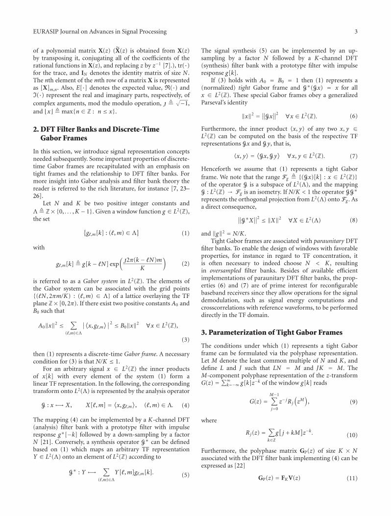
EURASIP Journal on Advances in Signal Processing 3
of a polynomial matrix X(z) (X(z) is obtained from X(z)by transposing it, conjugating all of the coefficients of therational functions in X(z), and replacing z by z−1 [7].), tr(·)for the trace, and IN denotes the identity matrix of size N .The nth element of the mth row of a matrix X is representedas [X]m,n. Also, E[·] denotes the expected value, R(·) andI(·) represent the real and imaginary parts, respectively, ofcomplex arguments, mod the modulo operation, j �
√−1,and x� � max{n ∈ Z : n ≤ x}.
2. DFT Filter Banks and Discrete-TimeGabor Frames
In this section, we introduce signal representation conceptsneeded subsequently. Some important properties of discrete-time Gabor frames are recapitulated with an emphasis ontight frames and the relationship to DFT filter banks. Formore insight into Gabor analysis and filter bank theory thereader is referred to the rich literature, for instance [7, 23–26].
Let N and K be two positive integer constants andΛ � Z×{0, . . . ,K − 1}. Given a window function g ∈ L2(Z),the set
{g�,m[k] : (�,m) ∈ Λ
}(1)
with
g�,m[k] � g[k − �N] exp(j2π(k − �N)m
K
)(2)
is referred to as a Gabor system in L2(Z). The elements ofthe Gabor system can be associated with the grid points{(�N , 2πm/K) : (�,m) ∈ Λ} of a lattice overlaying the TFplane Z× [0, 2π). If there exist two positive constants A0 andB0 such that
A0‖x‖2 ≤∑
(�,m)∈Λ
∣∣⟨x, g�,m⟩∣∣2 ≤ B0‖x‖2 ∀x ∈ L2(Z),
(3)
then (1) represents a discrete-time Gabor frame. A necessarycondition for (3) is that N/K ≤ 1.
For an arbitrary signal x ∈ L2(Z) the inner productsof x[k] with every element of the system (1) form alinear TF representation. In the following, the correspondingtransform onto L2(Λ) is represented by the analysis operator
G : x �−→ X , X[�,m] = ⟨x, g�,m⟩
, (�,m) ∈ Λ. (4)
The mapping (4) can be implemented by a K-channel DFT(analysis) filter bank with a prototype filter with impulseresponse g∗[−k] followed by a down-sampling by a factorN [21]. Conversely, a synthesis operator G∗ can be definedbased on (1) which maps an arbitrary TF representationY ∈ L2(Λ) onto an element of L2(Z) according to
G∗ : Y �−→∑
(�,m)∈ΛY[�,m]g�,m[k]. (5)
The signal synthesis (5) can be implemented by an up-sampling by a factor N followed by a K-channel DFT(synthesis) filter bank with a prototype filter with impulseresponse g[k].
If (3) holds with A0 = B0 = 1 then (1) represents a(normalized) tight Gabor frame and G∗(Gx) = x for allx ∈ L2(Z). These special Gabor frames obey a generalizedParseval’s identity
‖x‖2 = ∥∥Gx∥∥2 ∀x ∈ L2(Z). (6)
Furthermore, the inner product 〈x, y〉 of any two x, y ∈L2(Z) can be computed on the basis of the respective TFrepresentations Gx and Gy, that is,
〈x, y〉 = ⟨Gx, Gy⟩ ∀x, y ∈ L2(Z). (7)
Henceforth we assume that (1) represents a tight Gaborframe. We note that the range Fg � {(Gx)[k] : x ∈ L2(Z)}of the operator G is a subspace of L2(Λ), and the mappingG : L2(Z) → Fg is an isometry. If N/K < 1 the operator GG∗
represents the orthogonal projection from L2(Λ) onto Fg . Asa direct consequence,
∥∥G∗X∥∥2 ≤ ‖X‖2 ∀X ∈ L2(Λ) (8)
and ‖g‖2 = N/K .Tight Gabor frames are associated with paraunitary DFT
filter banks. To enable the design of windows with favorableproperties, for instance in regard to TF concentration, itis often necessary to indeed choose N < K , resultingin oversampled filter banks. Besides of available efficientimplementations of paraunitary DFT filter banks, the prop-erties (6) and (7) are of prime interest for reconfigurablebaseband receivers since they allow operations for the signaldemodulation, such as signal energy computations andcrosscorrelations with reference waveforms, to be performeddirectly in the TF domain.
3. Parameterization of Tight Gabor Frames
The conditions under which (1) represents a tight Gaborframe can be formulated via the polyphase representation.Let M denote the least common multiple of N and K , anddefine L and J such that LN = M and JK = M. TheM-component polyphase representation of the z-transformG(z) =∑∞
k=−∞ g[k]z−k of the window g[k] reads
G(z) =M−1∑
j=0
z− jRj
(zM)
, (9)
where
Rj(z) =∑
k∈Zg[j + kM
]z−k. (10)
Furthermore, the polyphase matrix GP(z) of size K × Nassociated with the DFT filter bank implementing (4) can beexpressed as [22]
GP(z) = FKV(z) (11)
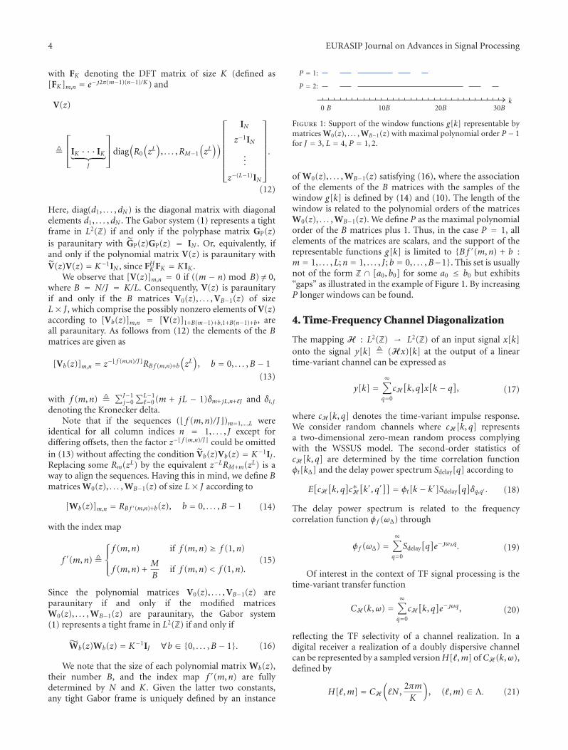
4 EURASIP Journal on Advances in Signal Processing
with FK denoting the DFT matrix of size K (defined as[FK ]m,n = e−j2π(m−1)(n−1)/K ) and
V(z)
�
⎡⎢⎣IK · · · IK︸ ︷︷ ︸
J
⎤⎥⎦diag
(R0
(zL)
, . . . ,RM−1
(zL))
⎡⎢⎢⎢⎢⎢⎢⎢⎣
IN
z−1IN
...
z−(L−1)IN
⎤⎥⎥⎥⎥⎥⎥⎥⎦
.
(12)
Here, diag(d1, . . . ,dN ) is the diagonal matrix with diagonalelements d1, . . . ,dN . The Gabor system (1) represents a tightframe in L2(Z) if and only if the polyphase matrix GP(z)is paraunitary with GP(z)GP(z) = IN . Or, equivalently, ifand only if the polynomial matrix V(z) is paraunitary withV(z)V(z) = K−1IN , since FHK FK = KIK .
We observe that [V(z)]m,n = 0 if ((m − n) mod B) /= 0,where B = N/J = K/L. Consequently, V(z) is paraunitaryif and only if the B matrices V0(z), . . . , VB−1(z) of sizeL× J , which comprise the possibly nonzero elements of V(z)according to [Vb(z)]m,n = [V(z)]1+B(m−1)+b,1+B(n−1)+b, areall paraunitary. As follows from (12) the elements of the Bmatrices are given as
[Vb(z)]m,n = z− f (m,n)/J�RB f (m,n)+b
(zL)
, b = 0, . . . ,B − 1
(13)
with f (m,n) � ∑J−1j=0
∑L−1�=0 (m + jL − 1)δm+ jL,n+�J and δi, j
denoting the Kronecker delta.Note that if the sequences ( f (m,n)/J�)m=1,...,L were
identical for all column indices n = 1, . . . , J except fordiffering offsets, then the factor z− f (m,n)/J� could be omittedin (13) without affecting the condition Vb(z)Vb(z) = K−1IJ .Replacing some Rm(zL) by the equivalent z−LRM+m(zL) is away to align the sequences. Having this in mind, we define Bmatrices W0(z), . . . , WB−1(z) of size L× J according to
[Wb(z)]m,n = RB f ′(m,n)+b(z), b = 0, . . . ,B − 1 (14)
with the index map
f ′(m,n) �
⎧⎪⎨⎪⎩
f (m,n) if f (m,n) ≥ f (1,n)
f (m,n) +M
Bif f (m,n) < f (1,n).
(15)
Since the polynomial matrices V0(z), . . . , VB−1(z) areparaunitary if and only if the modified matricesW0(z), . . . , WB−1(z) are paraunitary, the Gabor system(1) represents a tight frame in L2(Z) if and only if
Wb(z)Wb(z) = K−1IJ ∀b ∈ {0, . . . ,B − 1}. (16)
We note that the size of each polynomial matrix Wb(z),their number B, and the index map f ′(m,n) are fullydetermined by N and K . Given the latter two constants,any tight Gabor frame is uniquely defined by an instance
P = 1:
P = 2:
0 B 10B 20B 30Bk
Figure 1: Support of the window functions g[k] representable bymatrices W0(z), . . . , WB−1(z) with maximal polynomial order P − 1for J = 3, L = 4, P = 1, 2.
of W0(z), . . . , WB−1(z) satisfying (16), where the associationof the elements of the B matrices with the samples of thewindow g[k] is defined by (14) and (10). The length of thewindow is related to the polynomial orders of the matricesW0(z), . . . , WB−1(z). We define P as the maximal polynomialorder of the B matrices plus 1. Thus, in the case P = 1, allelements of the matrices are scalars, and the support of therepresentable functions g[k] is limited to {B f ′(m,n) + b :m = 1, . . . ,L;n = 1, . . . , J ; b = 0, . . . ,B−1}. This set is usuallynot of the form Z ∩ [a0, b0] for some a0 ≤ b0 but exhibits“gaps” as illustrated in the example of Figure 1. By increasingP longer windows can be found.
4. Time-Frequency Channel Diagonalization
The mapping H : L2(Z) → L2(Z) of an input signal x[k]onto the signal y[k] � (Hx)[k] at the output of a lineartime-variant channel can be expressed as
y[k] =∞∑
q=0
cH[k, q]x[k − q], (17)
where cH [k, q] denotes the time-variant impulse response.We consider random channels where cH [k, q] representsa two-dimensional zero-mean random process complyingwith the WSSUS model. The second-order statistics ofcH [k, q] are determined by the time correlation functionφt[kΔ] and the delay power spectrum Sdelay[q] according to
E[cH[k, q]c∗H[k′, q′
]] = φt[k − k′]Sdelay[q]δq,q′ . (18)
The delay power spectrum is related to the frequencycorrelation function φf (ωΔ) through
φf (ωΔ) =∞∑
q=0
Sdelay[q]e−jωΔq. (19)
Of interest in the context of TF signal processing is thetime-variant transfer function
CH (k,ω) =∞∑
q=0
cH[k, q]e−jωq, (20)
reflecting the TF selectivity of a channel realization. In adigital receiver a realization of a doubly dispersive channelcan be represented by a sampled versionH[�,m] ofCH (k,ω),defined by
H[�,m] = CH
(�N ,
2πmK
), (�,m) ∈ Λ. (21)
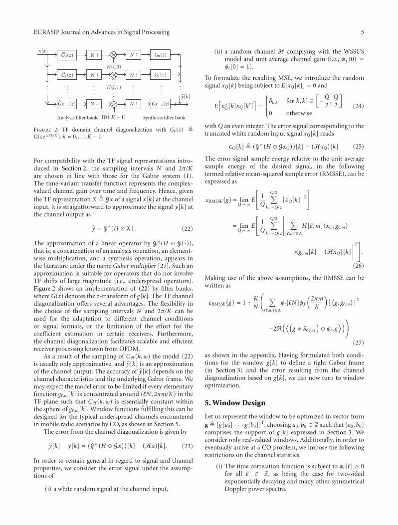
EURASIP Journal on Advances in Signal Processing 5
x[k]G0(z) N ↓
G1(z) N ↓...
......
GK−1(z) N ↓
Analysis filter bank
H(l, 0)
H(l, 1)...
H(l,K − 1)
N ↑
N ↑...
N ↑
G0(z)
G1(z)
...
GK−1(z)
y[k]
Synthesis filter bank
...
Figure 2: TF domain channel diagonalization with Gk(z) �G(zej2πk/K ), k = 0, . . . ,K − 1.
For compatibility with the TF signal representations intro-duced in Section 2, the sampling intervals N and 2π/Kare chosen in line with those for the Gabor system (1).The time-variant transfer function represents the complex-valued channel gain over time and frequency. Hence, giventhe TF representation X � Gx of a signal x[k] at the channelinput, it is straightforward to approximate the signal y[k] atthe channel output as
y = G∗(H � X). (22)
The approximation of a linear operator by G∗(H � G(·)),that is, a concatenation of an analysis operation, an element-wise multiplication, and a synthesis operation, appears inthe literature under the name Gabor multiplier [27]. Such anapproximation is suitable for operators that do not involveTF shifts of large magnitude (i.e., underspread operators).Figure 2 shows an implementation of (22) by filter banks,where G(z) denotes the z-transform of g[k]. The TF channeldiagonalization offers several advantages. The flexibility inthe choice of the sampling intervals N and 2π/K can beused for the adaptation to different channel conditionsor signal formats, or the limitation of the effort for thecoefficient estimation in certain receivers. Furthermore,the channel diagonalization facilitates scalable and efficientreceiver processing known from OFDM.
As a result of the sampling of CH (k,ω) the model (22)is usually only approximative, and y[k] is an approximationof the channel output. The accuracy of y[k] depends on thechannel characteristics and the underlying Gabor frame. Wemay expect the model error to be limited if every elementaryfunction g�,m[k] is concentrated around (�N , 2πm/K) in theTF plane such that CH (k,ω) is essentially constant withinthe sphere of g�,m[k]. Window functions fulfilling this can bedesigned for the typical underspread channels encounteredin mobile radio scenarios by CO, as shown in Section 5.
The error from the channel diagonalization is given by
y[k]− y[k] = (G∗(H � Gx))
[k]− (Hx)[k]. (23)
In order to remain general in regard to signal and channelproperties, we consider the error signal under the assump-tions of
(i) a white random signal at the channel input,
(ii) a random channel H complying with the WSSUSmodel and unit average channel gain (i.e., φf (0) =φt[0] = 1).
To formulate the resulting MSE, we introduce the randomsignal xQ[k] being subject to E[xQ[k]] = 0 and
E[x∗Q[k]xQ[k′]
]=
⎧⎪⎨⎪⎩δk,k′ for k, k′ ∈
[−Q
2,Q
2
]
0 otherwise(24)
withQ an even integer. The error signal corresponding to thetruncated white random input signal xQ[k] reads
εQ[k] �(G∗(H � GxQ
))[k]− (HxQ
)[k]. (25)
The error signal sample energy relative to the unit averagesample energy of the desired signal, in the followingtermed relative mean-squared sample error (RMSSE), can beexpressed as
εRMSSE(g)= lim
Q→∞E
⎡⎣ 1Q
Q/2∑
k=−Q/2
∣∣εQ[k]∣∣2
⎤⎦
= limQ→∞
E
⎡⎣ 1Q
Q/2∑
k=−Q/2
∣∣∣∣∣∣
∑
(�,m)∈ΛH[�,m]
⟨xQ, g�,m
⟩
×g�,m[k]− (HxQ)[k]
∣∣∣∣∣
2⎤⎦.
(26)
Making use of the above assumptions, the RMSSE can bewritten as
εRMSSE(g) = 1 +
K
N
⎛⎝∑
(�,m)∈Λφt[�N]φf
(2πmK
)∣∣⟨g, g�,m⟩∣∣2
−2R(⟨(
g ∗ Sdelay
)� φt, g
⟩)⎞⎠
(27)
as shown in the appendix. Having formulated both condi-tions for the window g[k] to define a tight Gabor frame(in Section 3) and the error resulting from the channeldiagonalization based on g[k], we can now turn to windowoptimization.
5. Window Design
Let us represent the window to be optimized in vector formg � [g[a0] · · · g[b0]]T, choosing a0, b0 ∈ Z such that [a0, b0]comprises the support of g[k] expressed in Section 3. Weconsider only real-valued windows. Additionally, in order toeventually arrive at a CO problem, we impose the followingrestrictions on the channel statistics.
(i) The time correlation function is subject to φt[�] ≥ 0for all � ∈ Z, as being the case for two-sidedexponentially decaying and many other symmetricalDoppler power spectra.
6 EURASIP Journal on Advances in Signal Processing
(ii) The frequency correlation function fulfillsφf (2πm/K) + φf (−2πm/K) ≥ 0 for allm ∈ {0, . . . ,K − 1}, as, for instance, in the caseof exponentially decaying delay power spectra.
We note that |〈g, g�,m〉|2 can be expressed as (gTR(C�,m)g)2 +(gTI(C�,m)g)2 and R(〈(g∗Sdelay)�φt, g〉) as gTR(D0)g withappropriate square matrices C�,m and D0. As a consequence,the objective function (27) can be expressed in the form
εRMSSE(
g) =
F∑
k=1
ck(
gTCkg)2
+ gTDg + 1 (28)
for some F ∈ N depending on the support of g[k], whereC1, . . . , CF , D are real matrices and the constants c1, . . . , cF arepositive given the above restrictions.
Next, we need to incorporate the constraints under whichεRMSSE(g) will be minimized. In order to formulate theconstraints (16) on the window in the time domain, it ishelpful to permute the samples in g. Let us introduce awindow (h[0], . . . ,h[T − 1]) of length T = LJPB defined as
h[k] = g[B f ′(m,n) + b +Mp
], k = 0, . . . ,T − 1 (29)
with m = (k mod L) + 1, n = (k mod LJ)/L� + 1,p = (k mod LJP)/(LJ)�, and b = k/(LJP)�. The matricesW0(z), . . . , WB−1(z) and the samples of the permuted win-dow are related through
[Wb(z)]m,n =P−1∑
p=0
h[L(J(bP + p
)+ n− 1
)+m− 1
]z−p.
(30)
With (30) we can now translate the polyphase domainconstraints (16) into constraints on the permuted windowdefined by h � [h[0] · · ·h[T − 1]]T .
(1) Case B = 1. There are J constraints of formhTA�h = K−1. The �th diagonal matrix A� of size LJP × LJPis defined as
[A�]m,n =
⎧⎪⎪⎪⎪⎪⎪⎪⎪⎨⎪⎪⎪⎪⎪⎪⎪⎪⎩
1 if m = n,
m ∈⋃
p=0,...,P−1
{(pJ + � − 1
)L + 1,
. . . ,(pJ + �
)L}
,
0 otherwise,
(31)
with � ∈ {1, . . . , J}. Additionally, there are J2P − (J + 1)J/2constraints of form hTA�h = 0. The corresponding matricesAJ+1, . . . , AJ2P−(J−1)J/2 can be defined as the elements of the setresulting from deleting duplicate elements and zero-matricesfrom{
A ∈ RLJP×LJP given as [A]m,n
= [A�]m− jL,n + [A�]m,n− jL : j = 1, . . . , JP; � = 1, . . . , J}
(32)
where in (32) we let [A�]m,n equal zero if eitherm /∈{1, . . . ,LJP} or n /∈{1, . . . ,LJP}.
(2) Case B > 1. From each of the above-defined matricesA1, . . . , AJ2P−(J−1)J/2, B unique block diagonal matrices ofdimension T × T are reproduced which contain the originalmatrix as one of the B diagonal blocks of dimensionLJP × LJP. Hence, there are W � B(J2P − (J − 1)J/2)constraints in total. The constraint matrices are mutuallyorthogonal in the sense that tr(A�AT
m) = 0 for � /=m.We can now formulate the optimization problem in the
form
minh∈RT
F∑
k=1
ck(
hT Ckh)2
+ hTDh
subject to hTA�h = d� , � = 1, . . . ,W ,
(33)
where C1, . . . , CF , D are the matrices resulting fromC1, . . . , CF , D by permuting the rows and columns inaccordance with (29), and d� ∈ {K−1, 0}. This problem isdifficult to tackle for large T . Let us thus introduce H � hhT
and reformulate the optimization problem as
minH∈ST
F∑
k=1
cktr2(
HCk
)+ tr(
HD)
subject to
⎧⎨⎩
tr(HA�) = d� , � = 1, . . . ,W
rank(H) = 1,
(34)
where ST denotes the vector space of symmetric matrices ofdimensionT×T . In (34) we have a convex objective function,however, the set {H ∈ ST : rank(H) = 1} is nonconvex.Resorting to semidefinite relaxation, we obtain
minH∈ST
F∑
k=1
cktr2(
HCk
)+ tr(
HD)
subject to
⎧⎨⎩
tr(HA�) = d� , � = 1, . . . ,W
H � 0
(35)
with H � 0 denoting that H is positive semidefinite. Since{H ∈ ST : H � 0} is a convex subset of ST , we nowhave a CO problem [28]. Having found a matrix H0 ∈ STcorresponding to a global minimum of (35), we have twopossible cases. If rank(H0) = 1, a solution h0 of (33) isreadily obtainable from h0hT0 = H0 and the optimal windowgCO[k] is found through (29). If rank(H0) > 1, which weobserve in most of the cases, rank reduction methods mustbe employed. We compute a possibly suboptimal windowgCO[k] by the following three steps.
(i) In order to reduce the rank to 1, we resort to thematrix H0 = (N/K)v0vH0 composed by the dominanteigenvector v0 of H0, since H0 is the matrix nearest toH0 in terms of the Frobenius norm [29].
(ii) We translate√N/Kv0 into a window g[k] taking the
sample permutation defined in (29) into account.
(iii) We finally obtain gCO[k] by the algorithm [30], whichyields a window defining a tight frame and at the
EURASIP Journal on Advances in Signal Processing 7
same time minimizes the distance to a given window(i.e., g[k]) in terms of the L2-norm.
Employing steepest descent methods for solving (35)may result in very slow convergence, whereas alternativemethods may not be applicable when the number of dimen-sions is large. Neglecting the quadratic terms in the objectivefunction leads to the simplified optimization problem
minH∈ST
tr(
HD)
subject to
⎧⎨⎩
tr(HA�) = d� , � = 1, . . . ,W
H � 0.
(36)
As shown in [6], the linear objective function tr(HD)reflects the mean-squared deviation of H �Gx from G(Hx),that is, the model error in the TF domain. Problems ofthe form (36) are dealt with by SDP, a subfield of CO.For the efficient solution of these optimization problemsa number of sophisticated software packages are widelyavailable. However, because generally (H�Gx−G(Hx)) /∈Fg
the windows resulting from solving (36) do not minimizethe time domain error signal, the magnitude of whichdetermines the performance of the channel diagonalization.
6. Numerical Results
We consider a WSSUS channel with an exponentially decay-ing delay power spectrum, the sampled version of whichreads
Sdelay[q] = u
(q)(
1− exp(− 1τRMS
))exp(− q
τRMS
)(37)
with u(q) denoting the unit step function and τRMS the rootmean-squared (RMS) delay spread [31]. As for the Dopplerpower spectrum, a two-sided exponentially decaying shape isassumed, which results in the time correlation function
φt[kΔ] = 1
1 + 2π2ν2RMS|kΔ|2
, (38)
where νRMS represents the RMS Doppler spread. Sincechoosing an oversampling factor K/N larger than oneincreases the degrees of freedom in the window design, werestrict our attention to scenarios with K > N , involvingoversampled filter banks. Figure 3 shows optimized windowfunctions for different channel conditions and their Fouriertransforms. The waveforms were obtained numerically bysolving (35) using interior point methods [28] for N = 24,K = 32, P = 2 amounting to a window length of 240samples. An RMS delay spread τRMS of 3 samples andan RMS Doppler spread νRMS of 0.001 samples−1 wereassumed in Figure 3(a), while τRMS = 3, νRMS = 0.01in Figure 3(b). The two shown optimized windows achieveRMSSEs (27) of −16.01 dB and −8.44 dB. Figures 3(c) and3(d) show the Fourier transforms of the optimized pulsesin (a) and (b), respectively, versus the normalized frequencyω/2π. Obviously, the optimized waveforms become more
concentrated in time domain as the Doppler spread increases(see Figure 3(b) versus Figure 3(a)). For increasing Dopplerspreads the coherence time of the channel decreases, and thetemporal support of the optimized window is reduced inorder to limit the RMSSE.
The RMSSEs (27) achievable by optimized windowsare shown in Figure 4 for the same lattice constants andsimilar types of delay/Doppler power spectra. The RMSdelay spread τRMS ranges between 0.5 and 8 samples whilethe RMS Doppler spread νRMS equals 0.01 samples−1. Forevery considered τRMS a window gCO[k] was obtained bynumerically solving the CO problem (35), and a windowgSDP[k] by solving (36) through SDP, where both approachesrequired the above-mentioned additional steps for rankreduction. The global minimum of the objective function in(35) at H = H0, that is prior to the rank reduction, servesas a lower bound in the figure. The offsets of εRMSSE(gCO)and εRMSSE(gSDP) from the lower bound reflect the impactof the rank reduction. Additionally, the figure shows theRMSSEs resulting from choosing a window gRRC[k] with aroot-raised-cosine (RRC) shaped magnitude spectrum withwidth 2π/K and roll-off factor K/N − 1. We choose thiswindow function for comparison because it does constitute atight Gabor frame while exhibiting superior TF localizationproperties compared to rectangularly shaped windows forinstance. Finally, for the verification of εRMSSE(gCO) thesignals y = Hx and y = G∗(H � (Gx)) were also obtainedby simulations involving filter banks based on the optimizedwindows gCO[k] and random signal and WSSUS channelgenerators, and the resulting error signal analyzed.
Obviously, solving (35) leads to better windows thansolving (36). The considerable offset of the RMSSEs fromthe lower bound for smaller τRMS indicates that here therank reduction has a significant impact on the windows. Weobserve that rank reduction generally has a limited effectwhen the delay and Doppler spreads are of similar extent,that is, when in the TF plane the delay spread relative to thesampling interval in time (i.e., τRMS/N) is of the same orderof magnitude as the Doppler spread relative to the samplinginterval in frequency (i.e., νRMS/K−1).
The relatively high RMSSEs found in Figure 4 are aresult of the product τRMSνRMS being in the order of 10−2, amuch larger value than encountered in typical mobile radioscenarios. In environments with such severe dispersion inboth time and frequency, the model error performance canactually be improved by increasing the oversampling factorK/N . This can be seen in Table 1, showing some εRMSSE(gCO)observed under the same conditions as above except forchoosing different lattice constants. An RMS delay spread of1 sample is assumed here. The performance clearly improveswith the oversampling factor.
7. Generic Matched Filter Receiver
The considered TF channel diagonalization does not rely ona particular signal format, making it suitable for applicationin multimode receivers [32]. The burst structures definedin the various standards for wireless communications differ
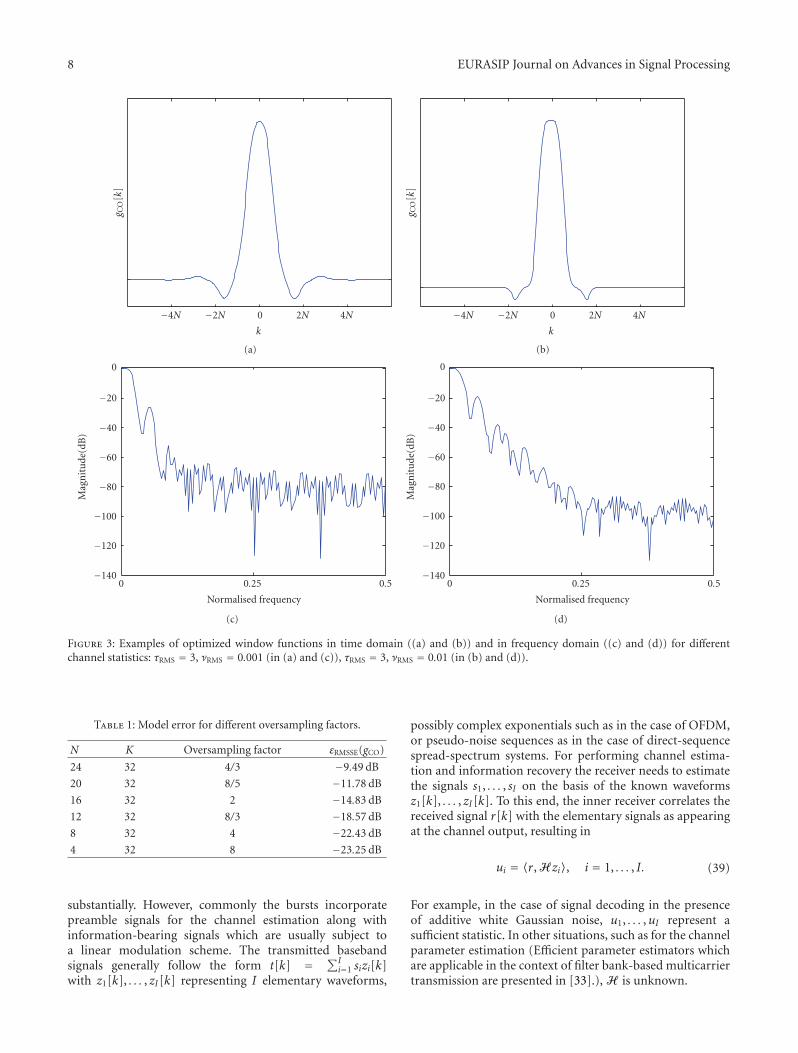
8 EURASIP Journal on Advances in Signal Processing
−4N −2N 0 2N 4N
k
g CO
[k]
(a)
−4N −2N 0 2N 4N
k
g CO
[k]
(b)
0 0.25 0.5
Normalised frequency
−140
−120
−100
−80
−60
−40
−20
0
Mag
nit
ude
(dB
)
(c)
0 0.25 0.5
Normalised frequency
−140
−120
−100
−80
−60
−40
−20
0
Mag
nit
ude
(dB
)
(d)
Figure 3: Examples of optimized window functions in time domain ((a) and (b)) and in frequency domain ((c) and (d)) for differentchannel statistics: τRMS = 3, νRMS = 0.001 (in (a) and (c)), τRMS = 3, νRMS = 0.01 (in (b) and (d)).
Table 1: Model error for different oversampling factors.
N K Oversampling factor εRMSSE(gCO)
24 32 4/3 −9.49 dB
20 32 8/5 −11.78 dB
16 32 2 −14.83 dB
12 32 8/3 −18.57 dB
8 32 4 −22.43 dB
4 32 8 −23.25 dB
substantially. However, commonly the bursts incorporatepreamble signals for the channel estimation along withinformation-bearing signals which are usually subject toa linear modulation scheme. The transmitted basebandsignals generally follow the form t[k] = ∑I
i=1 sizi[k]with z1[k], . . . , zI[k] representing I elementary waveforms,
possibly complex exponentials such as in the case of OFDM,or pseudo-noise sequences as in the case of direct-sequencespread-spectrum systems. For performing channel estima-tion and information recovery the receiver needs to estimatethe signals s1, . . . , sI on the basis of the known waveformsz1[k], . . . , zI[k]. To this end, the inner receiver correlates thereceived signal r[k] with the elementary signals as appearingat the channel output, resulting in
ui = 〈r, Hzi〉, i = 1, . . . , I. (39)
For example, in the case of signal decoding in the presenceof additive white Gaussian noise, u1, . . . ,uI represent asufficient statistic. In other situations, such as for the channelparameter estimation (Efficient parameter estimators whichare applicable in the context of filter bank-based multicarriertransmission are presented in [33].), H is unknown.
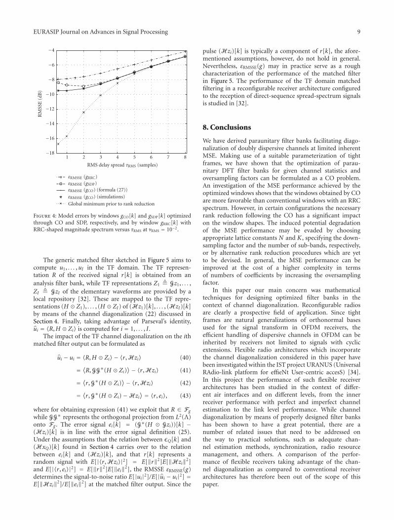
EURASIP Journal on Advances in Signal Processing 9
1 2 3 4 5 6 7 8
RMS delay spread τRMS (samples)
−18
−16
−14
−12
−10
−8
−6
−4
RM
SSE
(dB
)
εRMSSE (gRRC)εRMSSE (gSDP)εRMSSE (gCO) (formula (27))εRMSSE (gCO) (simulations)
Global minimum prior to rank reduction
Figure 4: Model errors by windows gCO[k] and gSDP[k] optimizedthrough CO and SDP, respectively, and by window gRRC[k] withRRC-shaped magnitude spectrum versus τRMS at νRMS = 10−2.
The generic matched filter sketched in Figure 5 aims tocompute u1, . . . ,uI in the TF domain. The TF represen-tation R of the received signal r[k] is obtained from ananalysis filter bank, while TF representations Z1 � Gz1, . . . ,ZI � GzI of the elementary waveforms are provided by alocal repository [32]. These are mapped to the TF repre-sentations (H � Z1), . . . , (H � ZI) of (Hz1)[k], . . . , (HzI)[k]by means of the channel diagonalization (22) discussed inSection 4. Finally, taking advantage of Parseval’s identity,ui = 〈R,H � Zi〉 is computed for i = 1, . . . , I .
The impact of the TF channel diagonalization on the ithmatched filter output can be formulated as
ui − ui = 〈R,H � Zi〉 − 〈r, Hzi〉 (40)
= ⟨R, GG∗(H � Zi)⟩− 〈r, Hzi〉 (41)
= ⟨r, G∗(H � Zi)⟩− 〈r, Hzi〉 (42)
= ⟨r, G∗(H � Zi)−Hzi⟩ = 〈r, ei〉, (43)
where for obtaining expression (41) we exploit that R ∈ Fg
while GG∗ represents the orthogonal projection from L2(Λ)onto Fg . The error signal ei[k] = (G∗(H � Gzi))[k] −(Hzi)[k] is in line with the error signal definition (25).Under the assumptions that the relation between εQ[k] and(HxQ)[k] found in Section 4 carries over to the relationbetween ei[k] and (Hzi)[k], and that r[k] represents arandom signal with E[|〈r, Hzi〉|2] = E[‖r‖2]E[‖Hzi‖2]and E[|〈r, ei〉|2] = E[‖r‖2]E[‖ei‖2], the RMSSE εRMSSE(g)determines the signal-to-noise ratio E[|ui|2]/E[|ui − ui|2] =E[‖Hzi‖2]/E[‖ei‖2] at the matched filter output. Since the
pulse (Hzi)[k] is typically a component of r[k], the afore-mentioned assumptions, however, do not hold in general.Nevertheless, εRMSSE(g) may in practice serve as a roughcharacterization of the performance of the matched filterin Figure 5. The performance of the TF domain matchedfiltering in a reconfigurable receiver architecture configuredto the reception of direct-sequence spread-spectrum signalsis studied in [32].
8. Conclusions
We have derived paraunitary filter banks facilitating diago-nalization of doubly dispersive channels at limited inherentMSE. Making use of a suitable parameterization of tightframes, we have shown that the optimization of parau-nitary DFT filter banks for given channel statistics andoversampling factors can be formulated as a CO problem.An investigation of the MSE performance achieved by theoptimized windows shows that the windows obtained by COare more favorable than conventional windows with an RRCspectrum. However, in certain configurations the necessaryrank reduction following the CO has a significant impacton the window shapes. The induced potential degradationof the MSE performance may be evaded by choosingappropriate lattice constants N and K , specifying the down-sampling factor and the number of sub-bands, respectively,or by alternative rank reduction procedures which are yetto be devised. In general, the MSE performance can beimproved at the cost of a higher complexity in termsof numbers of coefficients by increasing the oversamplingfactor.
In this paper our main concern was mathematicaltechniques for designing optimized filter banks in thecontext of channel diagonalization. Reconfigurable radiosare clearly a prospective field of application. Since tightframes are natural generalizations of orthonormal basesused for the signal transform in OFDM receivers, theefficient handling of dispersive channels in OFDM can beinherited by receivers not limited to signals with cyclicextensions. Flexible radio architectures which incorporatethe channel diagonalization considered in this paper havebeen investigated within the IST project URANUS (UniversalRAdio-link platform for effieNt User-centric accesS) [34].In this project the performance of such flexible receiverarchitectures has been studied in the context of differ-ent air interfaces and on different levels, from the innerreceiver performance with perfect and imperfect channelestimation to the link level performance. While channeldiagonalization by means of properly designed filter bankshas been shown to have a great potential, there are anumber of related issues that need to be addressed onthe way to practical solutions, such as adequate chan-nel estimation methods, synchronization, radio resourcemanagement, and others. A comparison of the perfor-mance of flexible receivers taking advantage of the chan-nel diagonalization as compared to conventional receiverarchitectures has therefore been out of the scope of thispaper.
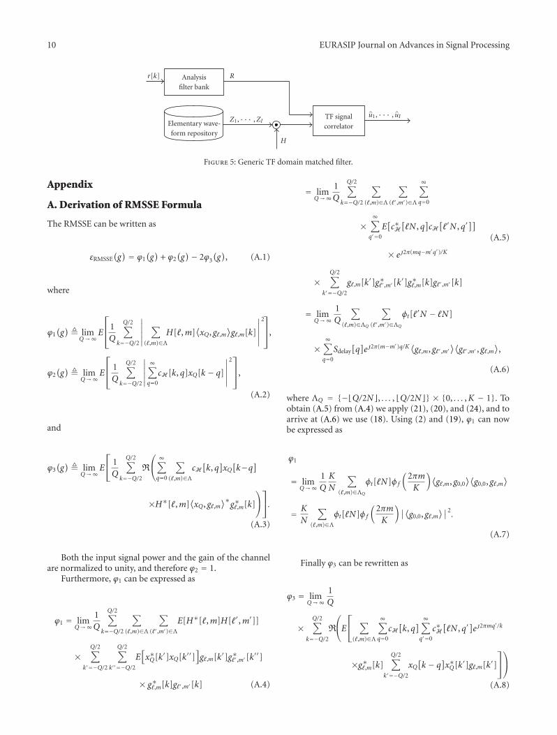
10 EURASIP Journal on Advances in Signal Processing
Analysisfilter bank
r[k] R
Elementary wave-form repository
Z1, · · · ,ZI
H
TF signalcorrelator
u1, · · · , uI
Figure 5: Generic TF domain matched filter.
Appendix
A. Derivation of RMSSE Formula
The RMSSE can be written as
εRMSSE(g) = ϕ1
(g)
+ ϕ2(g)− 2ϕ3
(g), (A.1)
where
ϕ1(g)
� limQ→∞
E
⎡⎢⎣
1Q
Q/2∑
k=−Q/2
∣∣∣∣∣∣
∑
(�,m)∈ΛH[�,m]
⟨xQ, g�,m
⟩g�,m[k]
∣∣∣∣∣∣
2⎤⎥⎦,
ϕ2(g)
� limQ→∞
E
⎡⎢⎣
1Q
Q/2∑
k=−Q/2
∣∣∣∣∣∣
∞∑
q=0
cH [k, q]xQ[k − q]
∣∣∣∣∣∣
2⎤⎥⎦,
(A.2)
and
ϕ3(g)
� limQ→∞
E
⎡⎣ 1Q
Q/2∑
k=−Q/2R
⎛⎝∞∑
q=0
∑
(�,m)∈ΛcH[k, q]xQ[k−q]
×H∗[�,m]⟨xQ, g�,m
⟩∗g∗�,m[k]
⎞⎠⎤⎦.
(A.3)
Both the input signal power and the gain of the channelare normalized to unity, and therefore ϕ2 = 1.
Furthermore, ϕ1 can be expressed as
ϕ1 = limQ→∞
1Q
Q/2∑
k=−Q/2
∑
(�,m)∈Λ
∑
(�′,m′)∈ΛE[H∗[�,m]H[�′,m′]]
×Q/2∑
k′=−Q/2
Q/2∑
k′′=−Q/2E[x∗Q[k′]xQ[k′′]
]g�,m[k′]g∗�′,m′[k′′]
× g∗�,m[k]g�′,m′[k] (A.4)
= limQ→∞
1Q
Q/2∑
k=−Q/2
∑
(�,m)∈Λ
∑
(�′,m′)∈Λ
∞∑
q=0
×∞∑
q′=0
E[c∗H[�N , q
]cH[�′N , q′
]]
× ej2π(mq−m′q′)/K
×Q/2∑
k′=−Q/2g�,m[k′]g∗�′,m′[k′]g∗�,m[k]g�′,m′[k]
(A.5)
= limQ→∞
1Q
∑
(�,m)∈ΛQ
∑
(�′,m′)∈ΛQ
φt[�′N − �N]
×∞∑
q=0
Sdelay[q]ej2π(m−m′)q/K⟨g�,m, g�′,m′
⟩⟨g�′,m′ , g�,m
⟩,
(A.6)
where ΛQ = {−Q/2N�, . . . , Q/2N�} × {0, . . . ,K − 1}. Toobtain (A.5) from (A.4) we apply (21), (20), and (24), and toarrive at (A.6) we use (18). Using (2) and (19), ϕ1 can nowbe expressed as
ϕ1
= limQ→∞
1Q
K
N
∑
(�,m)∈ΛQ
φt[�N]φf
(2πmK
)⟨g�,m, g0,0
⟩⟨g0,0, g�,m
⟩
= K
N
∑
(�,m)∈Λφt[�N]φf
(2πmK
)∣∣⟨g0,0, g�,m⟩∣∣2
.
(A.7)
Finally ϕ3 can be rewritten as
ϕ3 = limQ→∞
1Q
×Q/2∑
k=−Q/2R
⎛⎝E
⎡⎣∑
(�,m)∈Λ
∞∑
q=0
cH[k, q] ∞∑
q′=0
c∗H[�N , q′
]ej2πmq
′/k
×g∗�,m[k]Q/2∑
k′=−Q/2xQ[k − q]x∗Q[k′]g�,m[k′]
⎤⎦⎞⎠
(A.8)
EURASIP Journal on Advances in Signal Processing 11
= limQ→∞
1Q
×R
⎛⎝∑
(�,m)∈Λ
Q/2∑
k=−Q/2
∞∑
q=0
∞∑
q′=0
E[cH[k, q]c∗H[�N , q′
]]
×g∗�,m[k]ej2πmq′/kg�,m
[k − q]
⎞⎠
(A.9)
= limQ→∞
1Q
×R
⎛⎝∑
(�,m)∈ΛQ
Q/2∑
k=−Q/2
∞∑
q=0
φt[k − �N]
×Sdelay[q]g∗�,m[k]g�,m
[k−q]ej2πmq/k
⎞⎠
(A.10)
= limQ→∞
1Q
K
NR
⎛⎝
Q/2∑
k=−Q/2φt[k]
∞∑
q=0
Sdelay[q]g0,0[k−q]g∗0,0[k]
⎞⎠
(A.11)
= K
NR(⟨(
g0,0 ∗ Sdelay
)� φt, g0,0
⟩). (A.12)
We use (24) to obtain (A.9) from (A.8), and for thederivation of (A.10), (18) is applied. Thus, the RMSSE isgiven by
εRMSSE(g)
= 1 +K
N
⎛⎝∑
(�,m)∈Λφt[�N]φf
(2πmK
)∣∣⟨g, g�,m⟩∣∣2
−2R(⟨(
g ∗ Sdelay
)� φt, g
⟩)⎞⎠.
(A.13)
References
[1] H. Sari, G. Karam, and I. Jeanclaude, “Frequency-domainequalization of mobile radio and terrestrial broadcast chan-nels,” in Proceedings of IEEE Global Telecommunications Con-ference (GLOBECOM ’94), pp. 1–5, San Francisco, Calif, USA,November 1994.
[2] D. Falconer, S. L. Ariyavisitakul, A. Benyamin-Seeyar, andB. Eidson, “Frequency domain equalization for single-carrierbroadband wireless systems,” IEEE Communications Magazine,vol. 40, no. 4, pp. 58–66, 2002.
[3] I. Martoyo, Frequency domain equalization in CDMA detection,Ph.D. thesis, Institut fur Nachrichtentechnik, University ofKarlsruhe, 1995.
[4] F. Adachi, A. Nakajima, K. Takeda, et al., “Frequency-domainequalisation for block CDMA transmission,” European Trans-actions on Telecommunications, vol. 19, no. 5, pp. 553–560,2008.
[5] H. Bolcskei and F. Hlawatsch, “Discrete zak transformspolyphase transforms and applications,” IEEE Transactions onSignal Processing, vol. 45, no. 4, pp. 851–866, 1997.
[6] Z. Ju, T. Hunziker, and D. Dahlhaus, “Time-frequency param-eterization of doubly dispersive channels,” in Proceedings ofthe European Signal Processing Conference (EUSIPCO ’09),Glasgow, UK, August 2009.
[7] P. P. Vaidyanathan, Multirate Systems and Filter Banks,Prentice-Hall, Englewood Cliffs, NJ, USA, 1993.
[8] P. Jung and G. Wunder, “The WSSUS pulse design problem inmulticarrier transmission,” IEEE Transactions on Communica-tions, vol. 55, no. 10, pp. 1918–1928, 2007.
[9] S.-M. Phoong, Y. Chang, and C.-Y. Chen, “DFT-modulatedfilterbank transceivers for multipath fading channels,” IEEETransactions on Signal Processing, vol. 53, no. 1, pp. 182–192,2005.
[10] P. Jung and G. Wunder, “Iterative pulse shaping for Gaborsignaling in WSSUS channels,” in Proceedings of IEEE Work-shop on Signal Processing Advances in Wireless Communications(SPAWC ’04), pp. 368–372, Lisbon, Portugal, 2004.
[11] P. Schniter, “A new approach to multicarrier pulse designfor doubly-dispersive channels,” in Proceedings of the AllertonConference on Communication, Control, and Computing, Mon-ticello, Ill, USA, October 2003.
[12] T. Strohmer and S. Beaver, “Optimal OFDM design fortime-frequency dispersive channels,” IEEE Transactions onCommunications, vol. 51, no. 7, pp. 1111–1122, 2003.
[13] M. G. Bellanger, “Specification and design of a prototype filterfor filter bank based multicarrier transmission,” in Proceedingsof IEEE International Conference on Acoustics, Speech, andSignal Processing (ICASSP ’01), vol. 4, pp. 2417–2420, 2001.
[14] W. Kozek and A. F. Molisch, “Nonorthogonal pulseshapes formulticarrier communications in doubly dispersive channels,”IEEE Journal on Selected Areas in Communications, vol. 16, no.8, pp. 1579–1589, 1998.
[15] S. Houwen, T. Chen, and S. A. Norman, “Design of FIR multi-rate filter banks using convex optimization,” in Proceedings ofIEEE Pacific RIM Conference on Communications, Computers,and Signal Processing, vol. 1, pp. 469–472, Victoria, Canada,August 1997.
[16] J. Xu and T. Strohmer, “Pulse construction in OFDM systemsvia convex optimization,” IEEE Transactions on Communica-tions, vol. 56, no. 8, pp. 1225–1230, 2008.
[17] B. Borna and T. N. Davidson, “Efficient filter bank designfor filtered multitone modulation,” in Proceedings of IEEEInternational Conference on Communications, vol. 1, pp. 38–42, Paris, France, June 2004.
[18] M. R. Wilbur, T. N. Davidson, and J. P. Reilly, “Efficient designof oversampled NPR GDFT filterbanks,” IEEE Transactions onSignal Processing, vol. 52, no. 7, pp. 1947–1963, 2004.
[19] H. H. Kha, H. D. Tuan, and T. Q. Nguyen, “Efficient design ofcosine-modulated filter banks via convex optimization,” IEEETransactions on Signal Processing, vol. 57, no. 3, pp. 966–976,2009.
[20] A. Karmakar, A. Kumar, and R. K. Patney, “Design of anoptimal two-channel orthogonal filterbank using semidefiniteprogramming,” IEEE Signal Processing Letters, vol. 14, no. 10,pp. 692–694, 2007.
[21] H. Bolcskei, F. Hlawatsch, and H. G. Feichtinger, “Equivalenceof DFT filter banks and Gabor expansions,” in WaveletApplications in Signal and Image Processing III, vol. 2569 ofProceedings of SPIE, pp. 128–139, San Diego, Calif, USA, July1995.
[22] Z. Cvetkovic and M. Vetterli, “Tight Weyl-Heisenberg framesin �2(Z),” IEEE Transactions on Signal Processing, vol. 46, no. 5,pp. 1256–1259, 1998.
12 EURASIP Journal on Advances in Signal Processing
[23] H. G. Feichtinger and T. Strohmer, Gabor Analysis and Algo-rithms: Theory and Applications, Birkhauser, Boston, Mass,USA, 1998.
[24] K. Grochenig, Foundations of Time-Frequency Analysis,Birkhauser, Boston, Mass, USA, 2001.
[25] J. Kovacevic and A. Chebira, “Life beyond bases: the advent offrames (Part I),” IEEE Signal Processing Magazine, vol. 24, no.4, pp. 86–104, 2007.
[26] J. Kovacevic and A. Chebira, “Life beyond bases: the advent offrames (Part II),” IEEE Signal Processing Magazine, vol. 24, no.5, pp. 115–125, 2007.
[27] H. G. Feichtinger, M. Hampejs, and G. Kracher, “Approxima-tion of matrices by Gabor multipliers,” IEEE Signal ProcessingLetters, vol. 11, no. 11, pp. 883–886, 2004.
[28] S. Boyd and L. Vandenberghe, Convex Optimization, Cam-bridge University Press, Cambridge, UK, 2004.
[29] G. H. Golub and C. F. V. Loan, Matrix Computations, JohnsHopkins University Press, Baltimore, Md, USA, 3rd edition,1996.
[30] A. J. E. M. Janssen and P. L. Søndergaard, “Iterative algorithmsto approximate canonical Gabor windows: computationalaspects,” Journal of Fourier Analysis and Applications, vol. 13,no. 2, pp. 211–241, 2007.
[31] P. A. Bello, “Characterization of randomly time-variant linearchannels,” IEEE Transactions on Communications Systems, vol.11, pp. 360–393, 1963.
[32] T. Hunziker, Z. Ju, and D. Dahlhaus, “A reconfigurablebaseband receiver architecture based on time-frequency signalprocessing,” in Proceedings of the ICT Mobile and WirelessCommunications Summit, Santander, Spain, June 2009.
[33] T. Hunziker and S. Stefanatos, “Efficient two-dimensionalfilters for doubly-dispersive channel estimation in time-frequency signal processing,” in Proceedings of the 10th IEEEInternational Symposium on Spread Spectrum Techniques andApplications (ISSSTA ’08), pp. 381–385, Bologna, Italy, August2008.
[34] European research project IST-27960, URANUS (Univer-sal RAdio-link platform for efficieNt User-centric accesS),http://www.ist-uranus.org/.
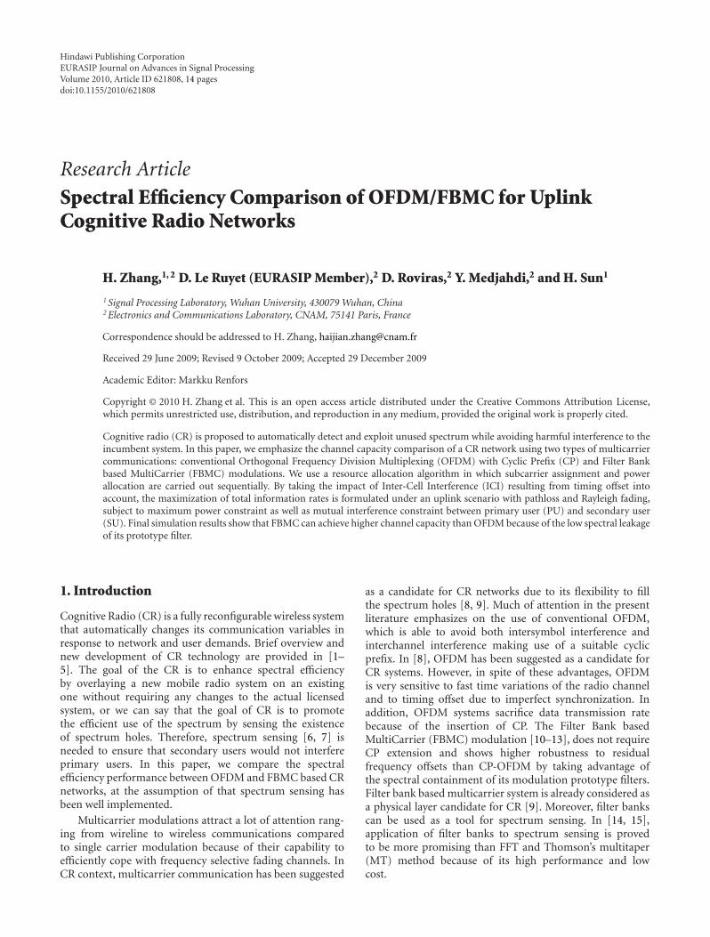
Hindawi Publishing CorporationEURASIP Journal on Advances in Signal ProcessingVolume 2010, Article ID 621808, 14 pagesdoi:10.1155/2010/621808
Research Article
Spectral Efficiency Comparison of OFDM/FBMC for UplinkCognitive Radio Networks
H. Zhang,1, 2 D. Le Ruyet (EURASIP Member),2 D. Roviras,2 Y. Medjahdi,2 and H. Sun1
1 Signal Processing Laboratory, Wuhan University, 430079 Wuhan, China2 Electronics and Communications Laboratory, CNAM, 75141 Paris, France
Correspondence should be addressed to H. Zhang, [email protected]
Received 29 June 2009; Revised 9 October 2009; Accepted 29 December 2009
Academic Editor: Markku Renfors
Copyright © 2010 H. Zhang et al. This is an open access article distributed under the Creative Commons Attribution License,which permits unrestricted use, distribution, and reproduction in any medium, provided the original work is properly cited.
Cognitive radio (CR) is proposed to automatically detect and exploit unused spectrum while avoiding harmful interference to theincumbent system. In this paper, we emphasize the channel capacity comparison of a CR network using two types of multicarriercommunications: conventional Orthogonal Frequency Division Multiplexing (OFDM) with Cyclic Prefix (CP) and Filter Bankbased MultiCarrier (FBMC) modulations. We use a resource allocation algorithm in which subcarrier assignment and powerallocation are carried out sequentially. By taking the impact of Inter-Cell Interference (ICI) resulting from timing offset intoaccount, the maximization of total information rates is formulated under an uplink scenario with pathloss and Rayleigh fading,subject to maximum power constraint as well as mutual interference constraint between primary user (PU) and secondary user(SU). Final simulation results show that FBMC can achieve higher channel capacity than OFDM because of the low spectral leakageof its prototype filter.
1. Introduction
Cognitive Radio (CR) is a fully reconfigurable wireless systemthat automatically changes its communication variables inresponse to network and user demands. Brief overview andnew development of CR technology are provided in [1–5]. The goal of the CR is to enhance spectral efficiencyby overlaying a new mobile radio system on an existingone without requiring any changes to the actual licensedsystem, or we can say that the goal of CR is to promotethe efficient use of the spectrum by sensing the existenceof spectrum holes. Therefore, spectrum sensing [6, 7] isneeded to ensure that secondary users would not interfereprimary users. In this paper, we compare the spectralefficiency performance between OFDM and FBMC based CRnetworks, at the assumption of that spectrum sensing hasbeen well implemented.
Multicarrier modulations attract a lot of attention rang-ing from wireline to wireless communications comparedto single carrier modulation because of their capability toefficiently cope with frequency selective fading channels. InCR context, multicarrier communication has been suggested
as a candidate for CR networks due to its flexibility to fillthe spectrum holes [8, 9]. Much of attention in the presentliterature emphasizes on the use of conventional OFDM,which is able to avoid both intersymbol interference andinterchannel interference making use of a suitable cyclicprefix. In [8], OFDM has been suggested as a candidate forCR systems. However, in spite of these advantages, OFDMis very sensitive to fast time variations of the radio channeland to timing offset due to imperfect synchronization. Inaddition, OFDM systems sacrifice data transmission ratebecause of the insertion of CP. The Filter Bank basedMultiCarrier (FBMC) modulation [10–13], does not requireCP extension and shows higher robustness to residualfrequency offsets than CP-OFDM by taking advantage ofthe spectral containment of its modulation prototype filters.Filter bank based multicarrier system is already considered asa physical layer candidate for CR [9]. Moreover, filter bankscan be used as a tool for spectrum sensing. In [14, 15],application of filter banks to spectrum sensing is provedto be more promising than FFT and Thomson’s multitaper(MT) method because of its high performance and lowcost.
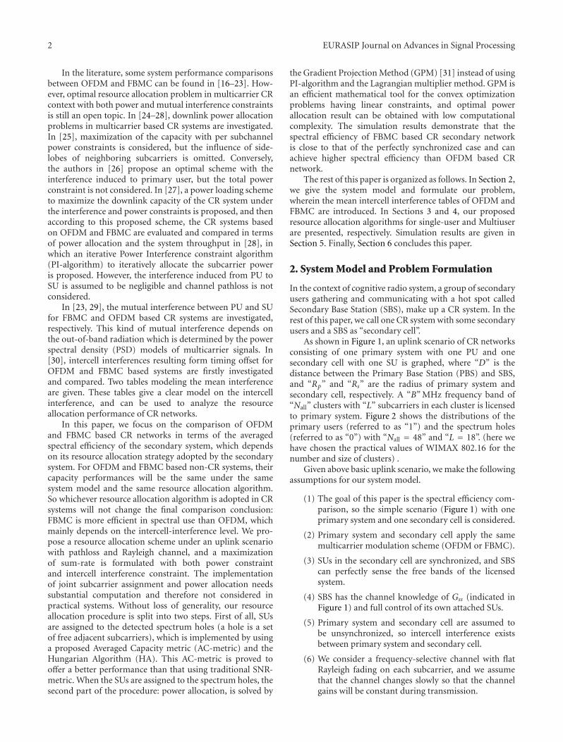
2 EURASIP Journal on Advances in Signal Processing
In the literature, some system performance comparisonsbetween OFDM and FBMC can be found in [16–23]. How-ever, optimal resource allocation problem in multicarrier CRcontext with both power and mutual interference constraintsis still an open topic. In [24–28], downlink power allocationproblems in multicarrier based CR systems are investigated.In [25], maximization of the capacity with per subchannelpower constraints is considered, but the influence of side-lobes of neighboring subcarriers is omitted. Conversely,the authors in [26] propose an optimal scheme with theinterference induced to primary user, but the total powerconstraint is not considered. In [27], a power loading schemeto maximize the downlink capacity of the CR system underthe interference and power constraints is proposed, and thenaccording to this proposed scheme, the CR systems basedon OFDM and FBMC are evaluated and compared in termsof power allocation and the system throughput in [28], inwhich an iterative Power Interference constraint algorithm(PI-algorithm) to iteratively allocate the subcarrier poweris proposed. However, the interference induced from PU toSU is assumed to be negligible and channel pathloss is notconsidered.
In [23, 29], the mutual interference between PU and SUfor FBMC and OFDM based CR systems are investigated,respectively. This kind of mutual interference depends onthe out-of-band radiation which is determined by the powerspectral density (PSD) models of multicarrier signals. In[30], intercell interferences resulting form timing offset forOFDM and FBMC based systems are firstly investigatedand compared. Two tables modeling the mean interferenceare given. These tables give a clear model on the intercellinterference, and can be used to analyze the resourceallocation performance of CR networks.
In this paper, we focus on the comparison of OFDMand FBMC based CR networks in terms of the averagedspectral efficiency of the secondary system, which dependson its resource allocation strategy adopted by the secondarysystem. For OFDM and FBMC based non-CR systems, theircapacity performances will be the same under the samesystem model and the same resource allocation algorithm.So whichever resource allocation algorithm is adopted in CRsystems will not change the final comparison conclusion:FBMC is more efficient in spectral use than OFDM, whichmainly depends on the intercell-interference level. We pro-pose a resource allocation scheme under an uplink scenariowith pathloss and Rayleigh channel, and a maximizationof sum-rate is formulated with both power constraintand intercell interference constraint. The implementationof joint subcarrier assignment and power allocation needssubstantial computation and therefore not considered inpractical systems. Without loss of generality, our resourceallocation procedure is split into two steps. First of all, SUsare assigned to the detected spectrum holes (a hole is a setof free adjacent subcarriers), which is implemented by usinga proposed Averaged Capacity metric (AC-metric) and theHungarian Algorithm (HA). This AC-metric is proved tooffer a better performance than that using traditional SNR-metric. When the SUs are assigned to the spectrum holes, thesecond part of the procedure: power allocation, is solved by
the Gradient Projection Method (GPM) [31] instead of usingPI-algorithm and the Lagrangian multiplier method. GPM isan efficient mathematical tool for the convex optimizationproblems having linear constraints, and optimal powerallocation result can be obtained with low computationalcomplexity. The simulation results demonstrate that thespectral efficiency of FBMC based CR secondary networkis close to that of the perfectly synchronized case and canachieve higher spectral efficiency than OFDM based CRnetwork.
The rest of this paper is organized as follows. In Section 2,we give the system model and formulate our problem,wherein the mean intercell interference tables of OFDM andFBMC are introduced. In Sections 3 and 4, our proposedresource allocation algorithms for single-user and Multiuserare presented, respectively. Simulation results are given inSection 5. Finally, Section 6 concludes this paper.
2. System Model and Problem Formulation
In the context of cognitive radio system, a group of secondaryusers gathering and communicating with a hot spot calledSecondary Base Station (SBS), make up a CR system. In therest of this paper, we call one CR system with some secondaryusers and a SBS as “secondary cell”.
As shown in Figure 1, an uplink scenario of CR networksconsisting of one primary system with one PU and onesecondary cell with one SU is graphed, where “D” is thedistance between the Primary Base Station (PBS) and SBS,and “Rp” and “Rs” are the radius of primary system andsecondary cell, respectively. A “B” MHz frequency band of“Nall” clusters with “L” subcarriers in each cluster is licensedto primary system. Figure 2 shows the distributions of theprimary users (referred to as “1”) and the spectrum holes(referred to as “0”) with “Nall = 48” and “L = 18”. (here wehave chosen the practical values of WIMAX 802.16 for thenumber and size of clusters) .
Given above basic uplink scenario, we make the followingassumptions for our system model.
(1) The goal of this paper is the spectral efficiency com-parison, so the simple scenario (Figure 1) with oneprimary system and one secondary cell is considered.
(2) Primary system and secondary cell apply the samemulticarrier modulation scheme (OFDM or FBMC).
(3) SUs in the secondary cell are synchronized, and SBScan perfectly sense the free bands of the licensedsystem.
(4) SBS has the channel knowledge of Gss (indicated inFigure 1) and full control of its own attached SUs.
(5) Primary system and secondary cell are assumed tobe unsynchronized, so intercell interference existsbetween primary system and secondary cell.
(6) We consider a frequency-selective channel with flatRayleigh fading on each subcarrier, and we assumethat the channel changes slowly so that the channelgains will be constant during transmission.
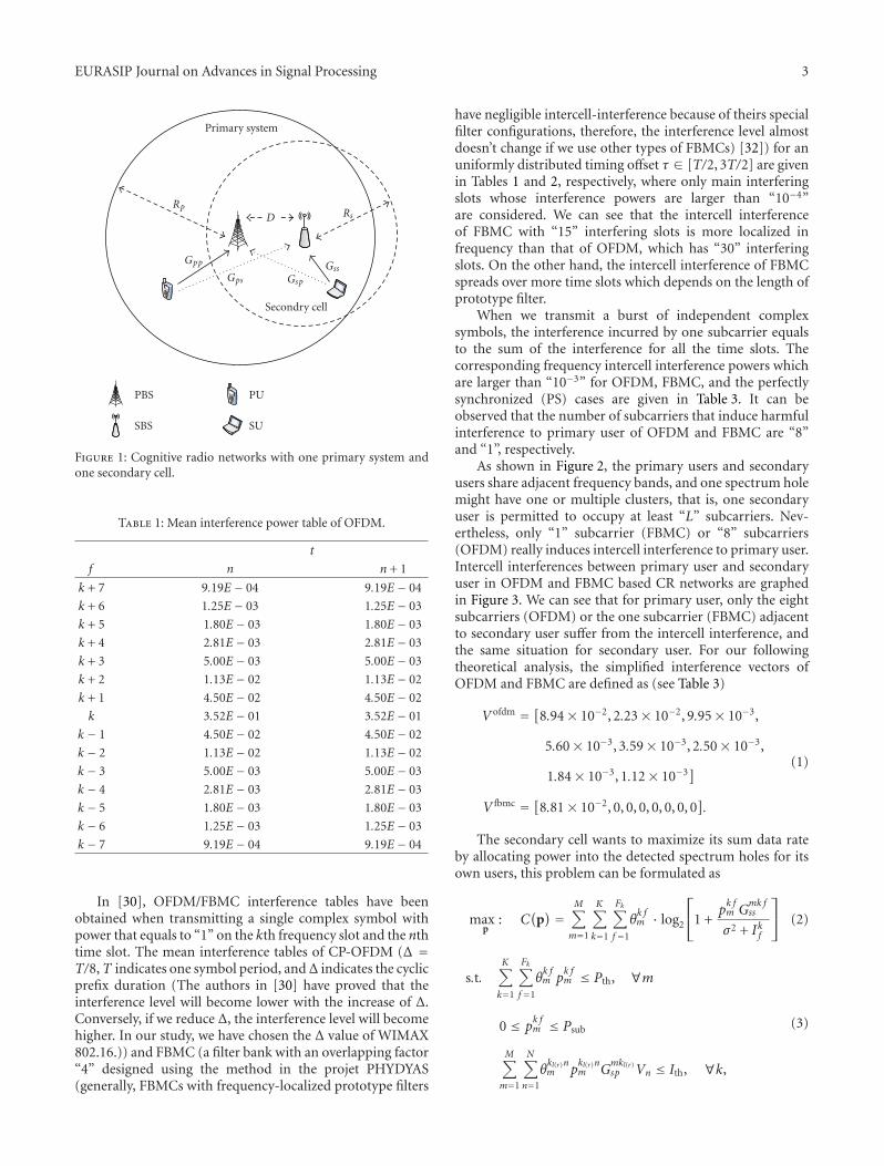
EURASIP Journal on Advances in Signal Processing 3
Primary system
Secondry cell
Gpp
Gps GspGss
DRp
Rs
PBS
SBS
PU
SU
Figure 1: Cognitive radio networks with one primary system andone secondary cell.
Table 1: Mean interference power table of OFDM.
t
f n n + 1
k + 7 9.19E − 04 9.19E − 04
k + 6 1.25E − 03 1.25E − 03
k + 5 1.80E − 03 1.80E − 03
k + 4 2.81E − 03 2.81E − 03
k + 3 5.00E − 03 5.00E − 03
k + 2 1.13E − 02 1.13E − 02
k + 1 4.50E − 02 4.50E − 02
k 3.52E − 01 3.52E − 01
k − 1 4.50E − 02 4.50E − 02
k − 2 1.13E − 02 1.13E − 02
k − 3 5.00E − 03 5.00E − 03
k − 4 2.81E − 03 2.81E − 03
k − 5 1.80E − 03 1.80E − 03
k − 6 1.25E − 03 1.25E − 03
k − 7 9.19E − 04 9.19E − 04
In [30], OFDM/FBMC interference tables have beenobtained when transmitting a single complex symbol withpower that equals to “1” on the kth frequency slot and the nthtime slot. The mean interference tables of CP-OFDM (Δ =T/8,T indicates one symbol period, andΔ indicates the cyclicprefix duration (The authors in [30] have proved that theinterference level will become lower with the increase of Δ.Conversely, if we reduce Δ, the interference level will becomehigher. In our study, we have chosen the Δ value of WIMAX802.16.)) and FBMC (a filter bank with an overlapping factor“4” designed using the method in the projet PHYDYAS(generally, FBMCs with frequency-localized prototype filters
have negligible intercell-interference because of theirs specialfilter configurations, therefore, the interference level almostdoesn’t change if we use other types of FBMCs) [32]) for anuniformly distributed timing offset τ ∈ [T/2, 3T/2] are givenin Tables 1 and 2, respectively, where only main interferingslots whose interference powers are larger than “10−4”are considered. We can see that the intercell interferenceof FBMC with “15” interfering slots is more localized infrequency than that of OFDM, which has “30” interferingslots. On the other hand, the intercell interference of FBMCspreads over more time slots which depends on the length ofprototype filter.
When we transmit a burst of independent complexsymbols, the interference incurred by one subcarrier equalsto the sum of the interference for all the time slots. Thecorresponding frequency intercell interference powers whichare larger than “10−3” for OFDM, FBMC, and the perfectlysynchronized (PS) cases are given in Table 3. It can beobserved that the number of subcarriers that induce harmfulinterference to primary user of OFDM and FBMC are “8”and “1”, respectively.
As shown in Figure 2, the primary users and secondaryusers share adjacent frequency bands, and one spectrum holemight have one or multiple clusters, that is, one secondaryuser is permitted to occupy at least “L” subcarriers. Nev-ertheless, only “1” subcarrier (FBMC) or “8” subcarriers(OFDM) really induces intercell interference to primary user.Intercell interferences between primary user and secondaryuser in OFDM and FBMC based CR networks are graphedin Figure 3. We can see that for primary user, only the eightsubcarriers (OFDM) or the one subcarrier (FBMC) adjacentto secondary user suffer from the intercell interference, andthe same situation for secondary user. For our followingtheoretical analysis, the simplified interference vectors ofOFDM and FBMC are defined as (see Table 3)
Vofdm = [8.94× 10⁻², 2.23× 10⁻², 9.95× 10⁻³,
5.60× 10⁻³, 3.59× 10⁻³, 2.50× 10⁻³,
1.84× 10⁻³, 1.12× 10⁻³]
V fbmc = [8.81× 10⁻², 0, 0, 0, 0, 0, 0, 0].
(1)
The secondary cell wants to maximize its sum data rateby allocating power into the detected spectrum holes for itsown users, this problem can be formulated as
max :p
C(
p) =
M∑
m=1
K∑
k=1
Fk∑
f=1
θk fm · log2
⎡⎣1 +
pk fm G
mk fss
σ2 + Ikf
⎤⎦ (2)
s.t.K∑
k=1
Fk∑
f=1
θk fm p
k fm ≤ Pth, ∀m
0 ≤ pk fm ≤ Psub
M∑
m=1
N∑
n=1
θkl(r)nm p
kl(r)nm G
mkl(r)sp Vn ≤ Ith, ∀k,
(3)
4 EURASIP Journal on Advances in Signal Processing
PU PU PU PU PUPU
1011· · ·00101 1
· · ·
48 clusters
1 2 · 18 1 2 · 18 1 2 · 18 1 2 · 18
Figure 2: Distributions of the primary users and the spectrum holes with “Nall = 48” and L=18.
Table 2: Mean interference power table of FBMC.
t
f n− 2 n− 1 n n + 1 n + 2
k − 1 1.08E − 03 1.99E − 02 4.60E − 02 1.99E − 02 1.08E − 03
k 1.05E − 03 1.26E − 01 5.69E − 01 1.26E − 01 1.05E − 03
k + 1 1.08E − 03 1.99E − 02 4.60E − 02 1.99E − 02 1.08E − 03
where M is the number of secondary users, K is the numberof spectrum holes, and Fk is the number of subcarriers in the
kth spectrum hole. θk fm ∈ {0, 1} is the subcarrier assignment
indicator, that is, θk fm = 1 if the f th subcarrier in the kth
spectrum hole is allocated to SU m, pk fm is the power of SU
m on the f th subcarrier in the kth spectrum hole, Gmk fss
is the propagation channel magnitude from SU m to SBSon the f th subcarrier in the kth spectrum hole, σ2 is thenoise power, and Ikf is the intercell interference from PU toSU on the f th subcarrier in the kth spectrum hole. Pth andPsub are the maximum user power limit and per subcarrierpower limit, respectively. N is the length of the interference
vector V , pkl(r)nm is the power of SU m on the left (right) nth
subcarrier in the kth spectrum hole,Gmkl(r)sp is the propagation
channel magnitude from SU m to PBS on the left (right) firstprimary subcarrier adjacent to the kth spectrum hole, andIth denotes the interference threshold prescribed by the PUon the first primary subcarrier adjacent to SU.
The intercell interference from PU to SU Ikf can beexpressed in the mathematical form as follows:
Ikf =
⎧⎪⎪⎪⎪⎪⎪⎪⎪⎪⎨⎪⎪⎪⎪⎪⎪⎪⎪⎪⎩
N∑
n= fPklp G
kl fps Vn, f = 1, 2, . . . N
N∑
n=Fk− f +1
Pkrp Gkr fps Vn, f = Fk −N + 1, . . . Fk
0, others,
(4)
where Pkl(r)p is the transmission power of PU located in the left
(right) of the kth spectrum hole, and Gkl(r) fps is the channel
magnitude from PU located in the left (right) of the kthspectrum hole to SBS on the f th subcarrier of the kthspectrum hole. Practically, the secondary cell is not capableof obtaining the transmission power of PU and the channelinformation from PU to SU, but Ikf can be measured during
Table 3: Intercell interference power tables for three different cases.
Cases
f OFDM FBMC PS
k + 8 1.12E − 3 0 0
k + 7 1.84E − 3 0 0
k + 6 2.50E − 3 0 0
k + 5 3.59E − 3 0 0
k + 4 5.60E − 3 0 0
k + 3 9.95E − 3 0 0
k + 2 2.23E − 2 0 0
k + 1 8.94E − 2 8.81E − 2 0
k 7.05E − 1 8.23E − 1 1
k − 1 8.94E − 2 8.81E − 2 0
k − 2 2.23E − 2 0 0
k − 3 9.95E − 3 0 0
k − 4 5.60E − 3 0 0
k − 5 3.59E − 3 0 0
k − 6 2.50E − 3 0 0
k − 7 1.84E − 3 0 0
k − 8 1.12E − 3 0 0
spectrum sensing by SBS without need to know any priorinformation.
In (3), the third inequality constraint is related tothe interference introduced by the secondary user to theprimary base station. This constraint is quite difficult tomanage because of the two following reasons: first of all,the threshold Ith has to be prescribed by the primarysystem. It represents the amount of interference that theprimary system can accept from secondary system. Standardsfor multicarriers CR systems are still under study and nocommon definition for interference threshold is availablein literature. Different thresholds corresponding to differentpenalties in terms of primary system capacity degradation
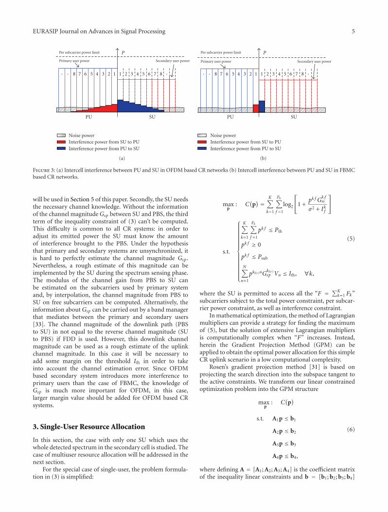
EURASIP Journal on Advances in Signal Processing 5
Secondary user powerPrimary user power
Per subcarrier power limit
PU SU
P
· · 8 7 6 5 4 3 2 1 1 2 3 4 5 6 7 8 ·
Noise powerInterference power from SU to PUInterference power from PU to SU
(a)
Secondary user powerPrimary user power
Per subcarrier power limit
PU SU
P
· · 8 7 6 5 4 3 2 1 1 2 3 4 5 6 7 8 ·
Noise powerInterference power from SU to PUInterference power from PU to SU
(b)
Figure 3: (a) Intercell interference between PU and SU in OFDM based CR networks (b) Intercell interference between PU and SU in FBMCbased CR networks.
will be used in Section 5 of this paper. Secondly, the SU needsthe necessary channel knowledge. Without the informationof the channel magnitude Gsp between SU and PBS, the thirdterm of the inequality constraint of (3) can’t be computed.This difficulty is common to all CR systems: in order toadjust its emitted power the SU must know the amountof interference brought to the PBS. Under the hypothesisthat primary and secondary systems are unsynchronized, itis hard to perfectly estimate the channel magnitude Gsp.Nevertheless, a rough estimate of this magnitude can beimplemented by the SU during the spectrum sensing phase.The modulus of the channel gain from PBS to SU canbe estimated on the subcarriers used by primary systemand, by interpolation, the channel magnitude from PBS toSU on free subcarriers can be computed. Alternatively, theinformation about Gsp can be carried out by a band managerthat mediates between the primary and secondary users[33]. The channel magnitude of the downlink path (PBSto SU) in not equal to the reverse channel magnitude (SUto PBS) if FDD is used. However, this downlink channelmagnitude can be used as a rough estimate of the uplinkchannel magnitude. In this case it will be necessary toadd some margin on the threshold Ith in order to takeinto account the channel estimation error. Since OFDMbased secondary system introduces more interference toprimary users than the case of FBMC, the knowledge ofGsp is much more important for OFDM, in this case,larger margin value should be added for OFDM based CRsystems.
3. Single-User Resource Allocation
In this section, the case with only one SU which uses thewhole detected spectrum in the secondary cell is studied. Thecase of multiuser resource allocation will be addressed in thenext section.
For the special case of single-user, the problem formula-tion in (3) is simplified:
maxp
: C(
p) =
K∑
k=1
Fk∑
f=1
log2
⎡⎣1 +
pk f Gk fss
σ2 + Ikf
⎤⎦
s.t.
⎧⎪⎪⎪⎪⎪⎪⎪⎪⎪⎪⎪⎪⎪⎨⎪⎪⎪⎪⎪⎪⎪⎪⎪⎪⎪⎪⎪⎩
K∑
k=1
Fk∑
f=1
pk f ≤ Pth
pk f ≥ 0
pk f ≤ Psub
N∑
n=1
pkl(r)nGkl(r)sp Vn ≤ Ith, ∀k,
(5)
where the SU is permitted to access all the “F = ∑Kk=1 Fk”
subcarriers subject to the total power constraint, per subcar-rier power constraint, as well as interference constraint.
In mathematical optimization, the method of Lagrangianmultipliers can provide a strategy for finding the maximumof (5), but the solution of extensive Lagrangian multipliersis computationally complex when “F” increases. Instead,herein the Gradient Projection Method (GPM) can beapplied to obtain the optimal power allocation for this simpleCR uplink scenario in a low computational complexity.
Rosen’s gradient projection method [31] is based onprojecting the search direction into the subspace tangent tothe active constraints. We transform our linear constrainedoptimization problem into the GPM structure
max :p
C(
p)
s.t. A1p ≤ b1
A2p ≤ b2
A3p ≤ b3
A4p ≤ b4,
(6)
where defining A = [A1; A2; A3; A4] is the coefficient matrixof the inequality linear constraints and b = [b1; b2; b3; b4]
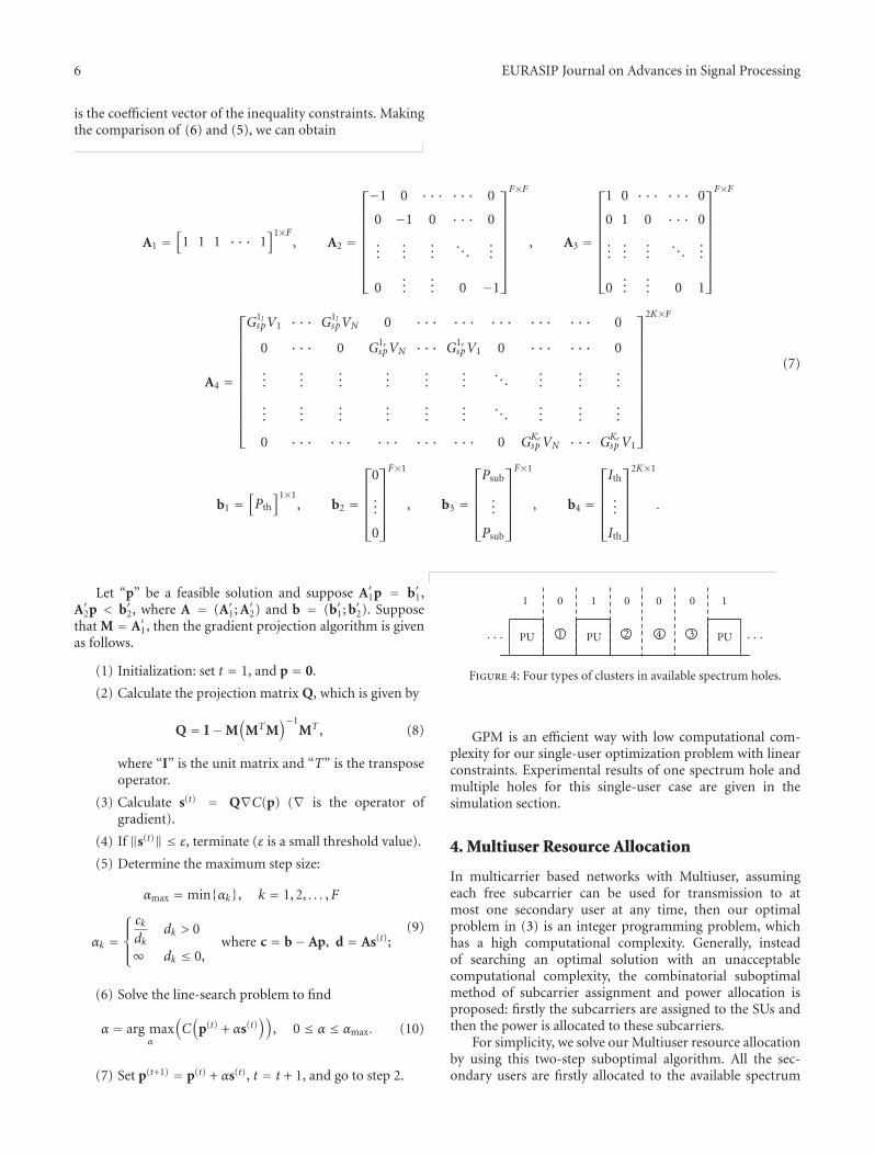
6 EURASIP Journal on Advances in Signal Processing
is the coefficient vector of the inequality constraints. Makingthe comparison of (6) and (5), we can obtain
A1 =[
1 1 1 · · · 1]1×F
, A2 =
⎡⎢⎢⎢⎢⎢⎢⎢⎢⎣
−1 0 · · · · · · 0
0 −1 0 · · · 0
......
.... . .
...
0...
... 0 −1
⎤⎥⎥⎥⎥⎥⎥⎥⎥⎦
F×F
, A3 =
⎡⎢⎢⎢⎢⎢⎢⎢⎢⎣
1 0 · · · · · · 0
0 1 0 · · · 0
......
.... . .
...
0...
... 0 1
⎤⎥⎥⎥⎥⎥⎥⎥⎥⎦
F×F
A4 =
⎡⎢⎢⎢⎢⎢⎢⎢⎢⎢⎢⎢⎢⎣
G1lspV1 · · · G1l
spVN 0 · · · · · · · · · · · · · · · 0
0 · · · 0 G1rspVN · · · G1r
spV1 0 · · · · · · 0
......
......
......
. . ....
......
......
......
......
. . ....
......
0 · · · · · · · · · · · · · · · 0 GKrspVN · · · GKr
spV1
⎤⎥⎥⎥⎥⎥⎥⎥⎥⎥⎥⎥⎥⎦
2K×F
b1 =[Pth
]1×1, b2 =
⎡⎢⎢⎢⎢⎣
0
...
0
⎤⎥⎥⎥⎥⎦
F×1
, b3 =
⎡⎢⎢⎢⎢⎣
Psub
...
Psub
⎤⎥⎥⎥⎥⎦
F×1
, b4 =
⎡⎢⎢⎢⎢⎣
Ith
...
Ith
⎤⎥⎥⎥⎥⎦
2K×1
.
(7)
Let “p” be a feasible solution and suppose A′1p = b′1,A′2p < b′2, where A = (A′1; A′2) and b = (b′1; b′2). Supposethat M = A′1, then the gradient projection algorithm is givenas follows.
(1) Initialization: set t = 1, and p = 0.
(2) Calculate the projection matrix Q, which is given by
Q = I−M(
MTM)−1
MT , (8)
where “I” is the unit matrix and “T” is the transposeoperator.
(3) Calculate s(t) = Q∇C(p) (∇ is the operator ofgradient).
(4) If ‖s(t)‖ ≤ ε, terminate (ε is a small threshold value).
(5) Determine the maximum step size:
αmax = min{αk}, k = 1, 2, . . . ,F
αk =
⎧⎪⎨⎪⎩
ckdk
dk > 0
∞ dk ≤ 0,where c = b− Ap, d = As(t);
(9)
(6) Solve the line-search problem to find
α = arg maxα
(C(
p(t) + αs(t)))
, 0 ≤ α ≤ αmax. (10)
(7) Set p(t+1) = p(t) + αs(t), t = t + 1, and go to step 2.
PU PU PU · · ·
1 0 1 0 0 0 1
1 2 4 3· · ·
Figure 4: Four types of clusters in available spectrum holes.
GPM is an efficient way with low computational com-plexity for our single-user optimization problem with linearconstraints. Experimental results of one spectrum hole andmultiple holes for this single-user case are given in thesimulation section.
4. Multiuser Resource Allocation
In multicarrier based networks with Multiuser, assumingeach free subcarrier can be used for transmission to atmost one secondary user at any time, then our optimalproblem in (3) is an integer programming problem, whichhas a high computational complexity. Generally, insteadof searching an optimal solution with an unacceptablecomputational complexity, the combinatorial suboptimalmethod of subcarrier assignment and power allocation isproposed: firstly the subcarriers are assigned to the SUs andthen the power is allocated to these subcarriers.
For simplicity, we solve our Multiuser resource allocationby using this two-step suboptimal algorithm. All the sec-ondary users are firstly allocated to the available spectrum
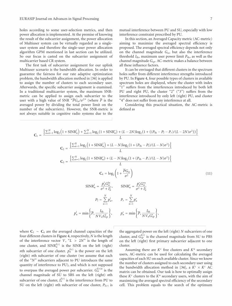
EURASIP Journal on Advances in Signal Processing 7
holes according to some user-selection metrics, and thenpower allocation is implemented. At the premise of knowingthe result of the subcarrier assignment, the power allocationof Multiuser system can be virtually regarded as a single-user system and therefore the single-user power allocationalgorithm GPM mentioned in last section can be utilized.So our focus is casted on the subcarrier assignment ofmulticarrier based CR system.
The first task of subcarrier assignment for our uplinkMultiuser scenario is the bandwidth allocation. In order toguarantee the fairness for our rate adaptive optimizationproblem, the bandwidth allocation method in [34] is appliedto assign the number of clusters to each secondary user.Afterwards, the specific subcarrier assignment is examined.In a traditional multicarrier system, the maximum SNR-metric can be applied to assign each subcarrier to theuser with a high value of SNR “PGss/σ2” (where P is theaveraged power by dividing the total power limit on thenumber of the subcarriers). However, the SNR-metric isnot always suitable in cognitive radio systems due to the
mutual interference between PU and SU, especially with lowinterference constraint prescribed by PU.
In this section, an Averaged Capacity metric (AC-metric)aiming to maximize the averaged spectral efficiency isproposed. The averaged spectral efficiency depends not onlyon the channel magnitude Gss, but also the interferencethreshold Ith, maximum user power limit Pth, as well as thechannel magnitude Gsp. AC-metric makes a balance betweenall these influence factors.
It can be envisaged that different clusters in the spectrumholes suffer from different interference strengths introducedby PU. In Figure 4, four possible types of clusters in availablespectrum holes are displayed, where the cluster with index“1” suffers from the interferences introduced by both leftPU and right PU, the cluster “2” (“3”) suffers from theinterference introduced by only left (right) PU, and cluster“4” does not suffer from any interference at all.
Considering this practical situation, the AC-metric isdefined as
C1 ={∑N
n=1 log2
(1 + SINRl
n
)+∑N
n=1 log2
(1 + SINRr
n
)+ (L− 2N)log2
(1 +
((Pth − Pl − Pr)/(L− 2N)σ2
))}
L
C2 ={∑N
n=1 log2
(1 + SINRl
n
)+ (L−N)log2
(1 + (Pth − Pl)/(L−N)σ2
)}
L
C3 ={∑N
n=1 log2
(1 + SINRr
n
)+ (L−N)log2
(1 + (Pth − Pr)/(L−N)σ2
)}
L
C4 = log2
(1 +
PGss
σ2
)
SINRln =
plnGlnss
σ2 + Iln, SINRr
n =prnG
rnss
σ2 + Irn
Pl =N∑
n=1
pln, Pr =N∑
n=1
prn
pln = min
{P,
IthNVnG
lsp
}, prn = min
{P,
IthNVnG
rsp
},
(11)
where C1 ∼ C4 are the averaged channel capacities of thefour different clusters in Figure 4, respectively,N is the lengthof the interference vector V , “L > 2N” is the length ofone cluster, and SINRl(r)
n is the SINR on the left (right)
nth subcarrier of one cluster. pl(r)n is the power on the left(right) nth subcarrier of one cluster (we assume that eachof the “N” subcarriers adjacent to PU introduces the samequantity of interference to PU), and which is not supposed
to overpass the averaged power per subcarrier. Gl(r)nss is the
channel magnitude of SU to SBS on the left (right) nth
subcarrier of one cluster, Il(r)n is the interference from PU toSU on the left (right) nth subcarrier of one cluster, Pl(r) is
the aggregated power on the left (right) N subcarriers of one
cluster, and Gl(r)sp is the channel magnitude from SU to PBS
on the left (right) first primary subcarrier adjacent to onecluster.
Assuming there are Kc free clusters and Ku secondaryusers, AC-metric can be used for calculating the averagedcapacities of each SU on each available cluster. Since we knowthe number of clusters assigned to each secondary user usingthe bandwidth allocation method in [34], a Kc × Kc ACmatrix can be obtained. Our task is how to optimally assignthese Kc clusters to the Ku secondary users, with the aim ofmaximizing the averaged spectral efficiency of the secondarycell. This problem equals to the search of the optimum
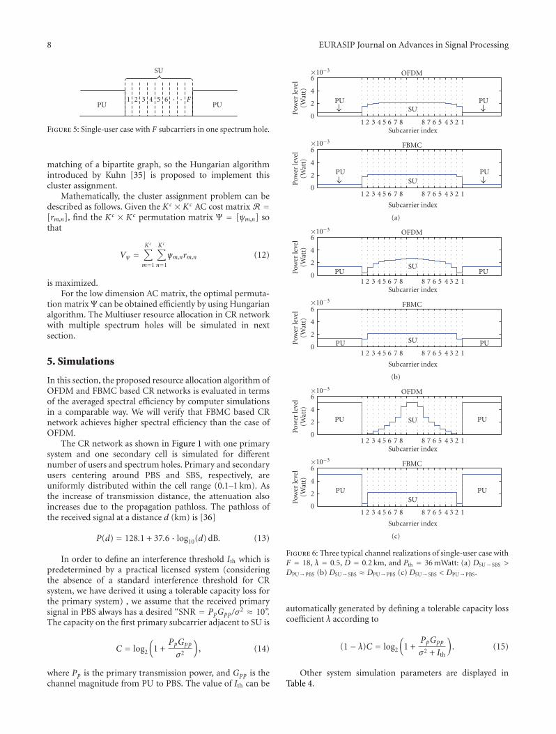
8 EURASIP Journal on Advances in Signal Processing
PU
SU
PU1 2 3 4 5 6 · · F
Figure 5: Single-user case with F subcarriers in one spectrum hole.
matching of a bipartite graph, so the Hungarian algorithmintroduced by Kuhn [35] is proposed to implement thiscluster assignment.
Mathematically, the cluster assignment problem can bedescribed as follows. Given the Kc × Kc AC cost matrix R =[rm,n], find the Kc × Kc permutation matrix Ψ = [ψm,n] sothat
Vψ =Kc∑
m=1
Kc∑
n=1
ψm,nrm,n (12)
is maximized.For the low dimension AC matrix, the optimal permuta-
tion matrixΨ can be obtained efficiently by using Hungarianalgorithm. The Multiuser resource allocation in CR networkwith multiple spectrum holes will be simulated in nextsection.
5. Simulations
In this section, the proposed resource allocation algorithm ofOFDM and FBMC based CR networks is evaluated in termsof the averaged spectral efficiency by computer simulationsin a comparable way. We will verify that FBMC based CRnetwork achieves higher spectral efficiency than the case ofOFDM.
The CR network as shown in Figure 1 with one primarysystem and one secondary cell is simulated for differentnumber of users and spectrum holes. Primary and secondaryusers centering around PBS and SBS, respectively, areuniformly distributed within the cell range (0.1–1 km). Asthe increase of transmission distance, the attenuation alsoincreases due to the propagation pathloss. The pathloss ofthe received signal at a distance d (km) is [36]
P(d) = 128.1 + 37.6 · log10(d) dB. (13)
In order to define an interference threshold Ith which ispredetermined by a practical licensed system (consideringthe absence of a standard interference threshold for CRsystem, we have derived it using a tolerable capacity loss forthe primary system) , we assume that the received primarysignal in PBS always has a desired “SNR = PpGpp/σ2 ≈ 10”.The capacity on the first primary subcarrier adjacent to SU is
C = log2
(1 +
PpGpp
σ2
), (14)
where Pp is the primary transmission power, and Gpp is thechannel magnitude from PU to PBS. The value of Ith can be
0
2
4
6×10⁻³
Pow
erle
vel
(Wat
t)
1 2 3 4 5 6 7 8 8 7 6 5 4 3 2 1
Subcarrier index
FBMC
PUPUSU
0
2
4
6×10⁻³
Pow
erle
vel
(Wat
t)
1 2 3 4 5 6 7 8 8 7 6 5 4 3 2 1Subcarrier index
OFDM
PUPUSU
(a)
0
2
4
6×10⁻³
Pow
erle
vel
(Wat
t)
1 2 3 4 5 6 7 8 8 7 6 5 4 3 2 1
Subcarrier index
FBMC
PUPU SU
0
2
4
6×10⁻³
Pow
erle
vel
(Wat
t)
1 2 3 4 5 6 7 8 8 7 6 5 4 3 2 1Subcarrier index
OFDM
PUPUSU
(b)
0
2
4
6×10⁻³
Pow
erle
vel
(Wat
t)
1 2 3 4 5 6 7 8 8 7 6 5 4 3 2 1
Subcarrier index
FBMC
PUPUSU
0
2
4
6×10⁻³
Pow
erle
vel
(Wat
t)
1 2 3 4 5 6 7 8 8 7 6 5 4 3 2 1Subcarrier index
OFDM
PUPU SU
(c)
Figure 6: Three typical channel realizations of single-user case withF = 18, λ = 0.5, D = 0.2 km, and Pth = 36 mWatt: (a) DSU→ SBS >DPU→PBS (b) DSU→ SBS ≈ DPU→PBS (c) DSU→ SBS < DPU→PBS.
automatically generated by defining a tolerable capacity losscoefficient λ according to
(1− λ)C = log2
(1 +
PpGpp
σ2 + Ith
). (15)
Other system simulation parameters are displayed inTable 4.
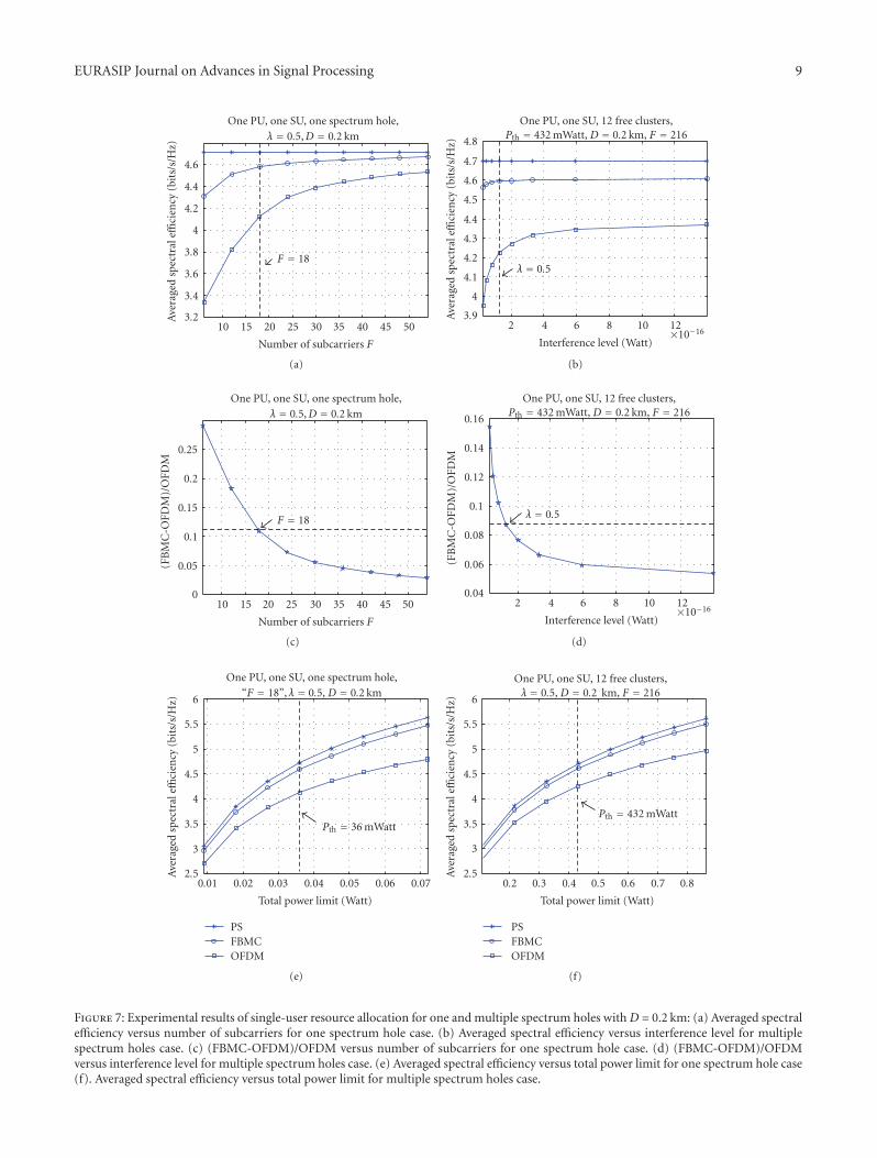
EURASIP Journal on Advances in Signal Processing 9
One PU, one SU, one spectrum hole,λ = 0.5,D = 0.2 km
3.2
3.4
3.6
3.8
4
4.2
4.4
4.6A
vera
ged
spec
tral
effici
ency
(bit
s/s/
Hz)
10 15 20 25 30 35 40 45 50
Number of subcarriers F
F = 18
(a)
One PU, one SU, 12 free clusters,Pth = 432 mWatt, D = 0.2 km, F = 216
3.9
4
4.1
4.2
4.3
4.4
4.5
4.6
4.7
4.8
Ave
rage
dsp
ectr
aleffi
cien
cy(b
its/
s/H
z)
2 4 6 8 10 12×10−16
Interference level (Watt)
λ = 0.5
(b)
One PU, one SU, one spectrum hole,λ = 0.5,D = 0.2 km
0
0.05
0.1
0.15
0.2
0.25
(FB
MC
-OFD
M)/
OFD
M
10 15 20 25 30 35 40 45 50
Number of subcarriers F
F = 18
(c)
One PU, one SU, 12 free clusters,Pth = 432 mWatt, D = 0.2 km, F = 216
0.04
0.06
0.08
0.1
0.12
0.14
0.16
(FB
MC
-OFD
M)/
OFD
M
2 4 6 8 10 12×10−16
Interference level (Watt)
λ = 0.5
(d)
One PU, one SU, one spectrum hole,“F = 18”, λ = 0.5, D = 0.2 km
2.5
3
3.5
4
4.5
5
5.5
6
Ave
rage
dsp
ectr
aleffi
cien
cy(b
its/
s/H
z)
0.01 0.02 0.03 0.04 0.05 0.06 0.07
Total power limit (Watt)
Pth = 36 mWatt
PSFBMCOFDM
(e)
One PU, one SU, 12 free clusters,λ = 0.5, D = 0.2 km, F = 216
2.5
3
3.5
4
4.5
5
5.5
6
Ave
rage
dsp
ectr
aleffi
cien
cy(b
its/
s/H
z)
0.2 0.3 0.4 0.5 0.6 0.7 0.8
Total power limit (Watt)
Pth = 432 mWatt
PSFBMCOFDM
(f)
Figure 7: Experimental results of single-user resource allocation for one and multiple spectrum holes withD = 0.2 km: (a) Averaged spectralefficiency versus number of subcarriers for one spectrum hole case. (b) Averaged spectral efficiency versus interference level for multiplespectrum holes case. (c) (FBMC-OFDM)/OFDM versus number of subcarriers for one spectrum hole case. (d) (FBMC-OFDM)/OFDMversus interference level for multiple spectrum holes case. (e) Averaged spectral efficiency versus total power limit for one spectrum hole case(f). Averaged spectral efficiency versus total power limit for multiple spectrum holes case.
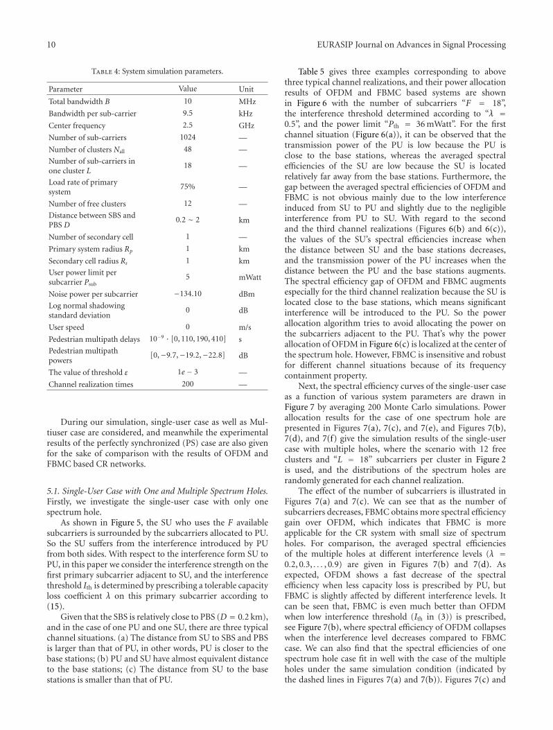
10 EURASIP Journal on Advances in Signal Processing
Table 4: System simulation parameters.
Parameter Value Unit
Total bandwidth B 10 MHz
Bandwidth per sub-carrier 9.5 kHz
Center frequency 2.5 GHz
Number of sub-carriers 1024 —
Number of clusters Nall 48 —
Number of sub-carriers inone cluster L
18 —
Load rate of primarysystem
75% —
Number of free clusters 12 —
Distance between SBS andPBS D
0.2 ∼ 2 km
Number of secondary cell 1 —
Primary system radius Rp 1 km
Secondary cell radius Rs 1 km
User power limit persubcarrier Psub
5 mWatt
Noise power per subcarrier −134.10 dBm
Log normal shadowingstandard deviation
0 dB
User speed 0 m/s
Pedestrian multipath delays 10−9 · [0, 110, 190, 410] s
Pedestrian multipathpowers
[0,−9.7,−19.2,−22.8] dB
The value of threshold ε 1e − 3 —
Channel realization times 200 —
During our simulation, single-user case as well as Mul-tiuser case are considered, and meanwhile the experimentalresults of the perfectly synchronized (PS) case are also givenfor the sake of comparison with the results of OFDM andFBMC based CR networks.
5.1. Single-User Case with One and Multiple Spectrum Holes.Firstly, we investigate the single-user case with only onespectrum hole.
As shown in Figure 5, the SU who uses the F availablesubcarriers is surrounded by the subcarriers allocated to PU.So the SU suffers from the interference introduced by PUfrom both sides. With respect to the interference form SU toPU, in this paper we consider the interference strength on thefirst primary subcarrier adjacent to SU, and the interferencethreshold Ith is determined by prescribing a tolerable capacityloss coefficient λ on this primary subcarrier according to(15).
Given that the SBS is relatively close to PBS (D = 0.2 km),and in the case of one PU and one SU, there are three typicalchannel situations. (a) The distance from SU to SBS and PBSis larger than that of PU, in other words, PU is closer to thebase stations; (b) PU and SU have almost equivalent distanceto the base stations; (c) The distance from SU to the basestations is smaller than that of PU.
Table 5 gives three examples corresponding to abovethree typical channel realizations, and their power allocationresults of OFDM and FBMC based systems are shownin Figure 6 with the number of subcarriers “F = 18”,the interference threshold determined according to “λ =0.5”, and the power limit “Pth = 36 mWatt”. For the firstchannel situation (Figure 6(a)), it can be observed that thetransmission power of the PU is low because the PU isclose to the base stations, whereas the averaged spectralefficiencies of the SU are low because the SU is locatedrelatively far away from the base stations. Furthermore, thegap between the averaged spectral efficiencies of OFDM andFBMC is not obvious mainly due to the low interferenceinduced from SU to PU and slightly due to the negligibleinterference from PU to SU. With regard to the secondand the third channel realizations (Figures 6(b) and 6(c)),the values of the SU’s spectral efficiencies increase whenthe distance between SU and the base stations decreases,and the transmission power of the PU increases when thedistance between the PU and the base stations augments.The spectral efficiency gap of OFDM and FBMC augmentsespecially for the third channel realization because the SU islocated close to the base stations, which means significantinterference will be introduced to the PU. So the powerallocation algorithm tries to avoid allocating the power onthe subcarriers adjacent to the PU. That’s why the powerallocation of OFDM in Figure 6(c) is localized at the center ofthe spectrum hole. However, FBMC is insensitive and robustfor different channel situations because of its frequencycontainment property.
Next, the spectral efficiency curves of the single-user caseas a function of various system parameters are drawn inFigure 7 by averaging 200 Monte Carlo simulations. Powerallocation results for the case of one spectrum hole arepresented in Figures 7(a), 7(c), and 7(e), and Figures 7(b),7(d), and 7(f) give the simulation results of the single-usercase with multiple holes, where the scenario with 12 freeclusters and “L = 18” subcarriers per cluster in Figure 2is used, and the distributions of the spectrum holes arerandomly generated for each channel realization.
The effect of the number of subcarriers is illustrated inFigures 7(a) and 7(c). We can see that as the number ofsubcarriers decreases, FBMC obtains more spectral efficiencygain over OFDM, which indicates that FBMC is moreapplicable for the CR system with small size of spectrumholes. For comparison, the averaged spectral efficienciesof the multiple holes at different interference levels (λ =0.2, 0.3, . . . , 0.9) are given in Figures 7(b) and 7(d). Asexpected, OFDM shows a fast decrease of the spectralefficiency when less capacity loss is prescribed by PU, butFBMC is slightly affected by different interference levels. Itcan be seen that, FBMC is even much better than OFDMwhen low interference threshold (Ith in (3)) is prescribed,see Figure 7(b), where spectral efficiency of OFDM collapseswhen the interference level decreases compared to FBMCcase. We can also find that the spectral efficiencies of onespectrum hole case fit in well with the case of the multipleholes under the same simulation condition (indicated bythe dashed lines in Figures 7(a) and 7(b)). Figures 7(c) and
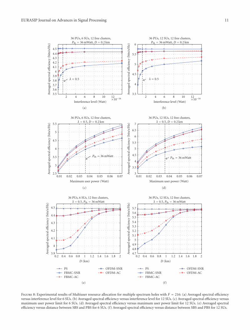
EURASIP Journal on Advances in Signal Processing 11
36 PUs, 6 SUs, 12 free clusters,Pth = 36 mWatt, D = 0.2 km
3.5
3.6
3.7
3.8
3.9
4
4.1
4.2
4.34.4
4.5A
vera
ged
spec
tral
effici
ency
(bit
s/s/
Hz)
2 4 6 8 10 12×10−16
Interference level (Watt)
λ = 0.5
(a)
36 PUs, 12 SUs, 12 free clusters,Pth = 36 mWatt, D = 0.2 km
3.5
4
4.5
5
5.5
6
Ave
rage
dsp
ectr
aleffi
cien
cy(b
its/
s/H
z)
2 4 6 8 10 12×10−16
Interference level (Watt)
λ = 0.5
(b)
36 PUs, 6 SUs, 12 free clusters,λ = 0.5, D = 0.2 km
2.5
3
3.5
4
4.5
5
5.5
Ave
rage
dsp
ectr
aleffi
cien
cy(b
its/
s/H
z)
0.01 0.02 0.03 0.04 0.05 0.06 0.07
Maximum user power (Watt)
Pth = 36 mWatt
(c)
36 PUs, 12 SUs, 12 free clusters,λ = 0.5, D = 0.2 km
3
3.5
4
4.5
5
5.5
6
6.5
7
Ave
rage
dsp
ectr
aleffi
cien
cy(b
its/
s/H
z)
0.01 0.02 0.03 0.04 0.05 0.06 0.07
Maximum user power (Watt)
Pth = 36 mWatt
(d)
36 PUs, 6 SUs, 12 free clusters,λ = 0.5, Pth = 36 mWatt
3.9
4
4.1
4.2
4.3
4.4
4.5
Ave
rage
dsp
ectr
aleffi
cien
cy(b
its/
s/H
z)
0.2 0.4 0.6 0.8 1 1.2 1.4 1.6 1.8 2
D (km)
PSFBMC-SNRFBMC-AC
OFDM-SNROFDM-AC
(e)
36 PUs, 12 SUs, 12 free clusters,λ = 0.5, Pth = 36 mWatt
4.74.8
4.9
5
5.1
5.2
5.3
5.4
5.5
5.6
5.7
Ave
rage
dsp
ectr
aleffi
cien
cy(b
its/
s/H
z)
0.2 0.4 0.6 0.8 1 1.2 1.4 1.6 1.8 2
D (km)
PSFBMC-SNRFBMC-AC
OFDM-SNROFDM-AC
(f)
Figure 8: Experimental results of Multiuser resource allocation for multiple spectrum holes with F = 216: (a) Averaged spectral efficiencyversus interference level for 6 SUs. (b) Averaged spectral efficiency versus interference level for 12 SUs. (c) Averaged spectral efficiency versusmaximum user power limit for 6 SUs. (d) Averaged spectral efficiency versus maximum user power limit for 12 SUs. (e) Averaged spectralefficiency versus distance between SBS and PBS for 6 SUs. (f) Averaged spectral efficiency versus distance between SBS and PBS for 12 SUs.
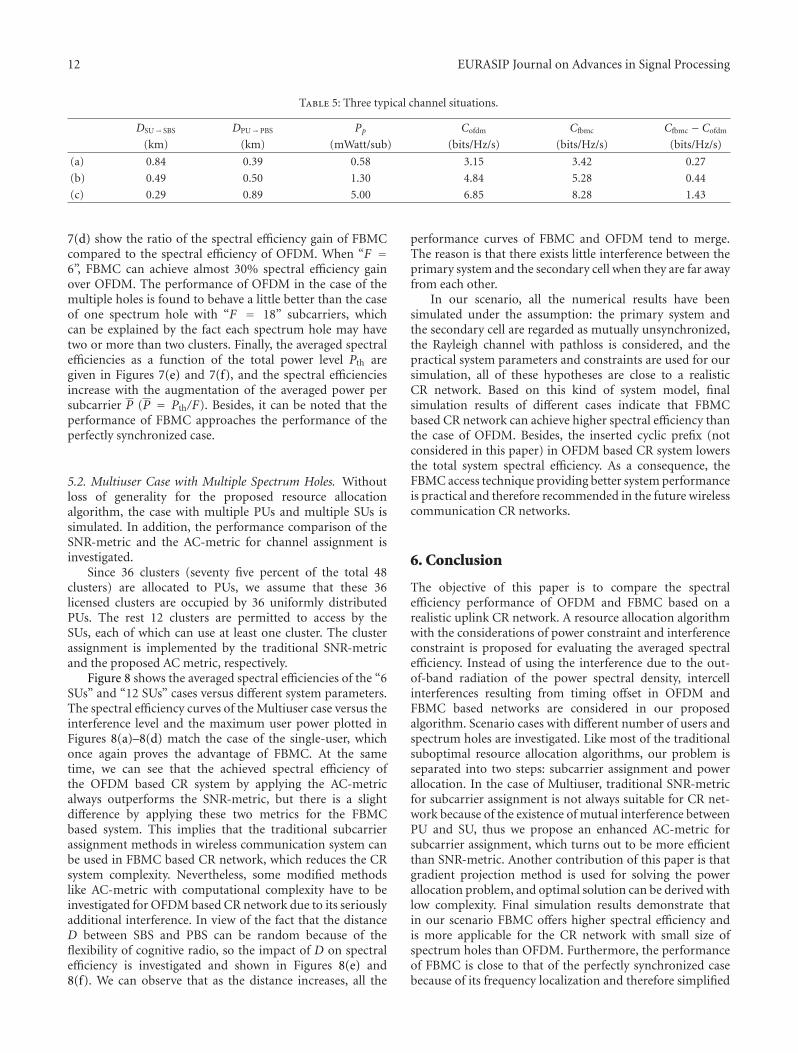
12 EURASIP Journal on Advances in Signal Processing
Table 5: Three typical channel situations.
DSU→ SBS DPU→PBS Pp Cofdm Cfbmc Cfbmc − Cofdm
(km) (km) (mWatt/sub) (bits/Hz/s) (bits/Hz/s) (bits/Hz/s)
(a) 0.84 0.39 0.58 3.15 3.42 0.27
(b) 0.49 0.50 1.30 4.84 5.28 0.44
(c) 0.29 0.89 5.00 6.85 8.28 1.43
7(d) show the ratio of the spectral efficiency gain of FBMCcompared to the spectral efficiency of OFDM. When “F =6”, FBMC can achieve almost 30% spectral efficiency gainover OFDM. The performance of OFDM in the case of themultiple holes is found to behave a little better than the caseof one spectrum hole with “F = 18” subcarriers, whichcan be explained by the fact each spectrum hole may havetwo or more than two clusters. Finally, the averaged spectralefficiencies as a function of the total power level Pth aregiven in Figures 7(e) and 7(f), and the spectral efficienciesincrease with the augmentation of the averaged power persubcarrier P (P = Pth/F). Besides, it can be noted that theperformance of FBMC approaches the performance of theperfectly synchronized case.
5.2. Multiuser Case with Multiple Spectrum Holes. Withoutloss of generality for the proposed resource allocationalgorithm, the case with multiple PUs and multiple SUs issimulated. In addition, the performance comparison of theSNR-metric and the AC-metric for channel assignment isinvestigated.
Since 36 clusters (seventy five percent of the total 48clusters) are allocated to PUs, we assume that these 36licensed clusters are occupied by 36 uniformly distributedPUs. The rest 12 clusters are permitted to access by theSUs, each of which can use at least one cluster. The clusterassignment is implemented by the traditional SNR-metricand the proposed AC metric, respectively.
Figure 8 shows the averaged spectral efficiencies of the “6SUs” and “12 SUs” cases versus different system parameters.The spectral efficiency curves of the Multiuser case versus theinterference level and the maximum user power plotted inFigures 8(a)–8(d) match the case of the single-user, whichonce again proves the advantage of FBMC. At the sametime, we can see that the achieved spectral efficiency ofthe OFDM based CR system by applying the AC-metricalways outperforms the SNR-metric, but there is a slightdifference by applying these two metrics for the FBMCbased system. This implies that the traditional subcarrierassignment methods in wireless communication system canbe used in FBMC based CR network, which reduces the CRsystem complexity. Nevertheless, some modified methodslike AC-metric with computational complexity have to beinvestigated for OFDM based CR network due to its seriouslyadditional interference. In view of the fact that the distanceD between SBS and PBS can be random because of theflexibility of cognitive radio, so the impact of D on spectralefficiency is investigated and shown in Figures 8(e) and8(f). We can observe that as the distance increases, all the
performance curves of FBMC and OFDM tend to merge.The reason is that there exists little interference between theprimary system and the secondary cell when they are far awayfrom each other.
In our scenario, all the numerical results have beensimulated under the assumption: the primary system andthe secondary cell are regarded as mutually unsynchronized,the Rayleigh channel with pathloss is considered, and thepractical system parameters and constraints are used for oursimulation, all of these hypotheses are close to a realisticCR network. Based on this kind of system model, finalsimulation results of different cases indicate that FBMCbased CR network can achieve higher spectral efficiency thanthe case of OFDM. Besides, the inserted cyclic prefix (notconsidered in this paper) in OFDM based CR system lowersthe total system spectral efficiency. As a consequence, theFBMC access technique providing better system performanceis practical and therefore recommended in the future wirelesscommunication CR networks.
6. Conclusion
The objective of this paper is to compare the spectralefficiency performance of OFDM and FBMC based on arealistic uplink CR network. A resource allocation algorithmwith the considerations of power constraint and interferenceconstraint is proposed for evaluating the averaged spectralefficiency. Instead of using the interference due to the out-of-band radiation of the power spectral density, intercellinterferences resulting from timing offset in OFDM andFBMC based networks are considered in our proposedalgorithm. Scenario cases with different number of users andspectrum holes are investigated. Like most of the traditionalsuboptimal resource allocation algorithms, our problem isseparated into two steps: subcarrier assignment and powerallocation. In the case of Multiuser, traditional SNR-metricfor subcarrier assignment is not always suitable for CR net-work because of the existence of mutual interference betweenPU and SU, thus we propose an enhanced AC-metric forsubcarrier assignment, which turns out to be more efficientthan SNR-metric. Another contribution of this paper is thatgradient projection method is used for solving the powerallocation problem, and optimal solution can be derived withlow complexity. Final simulation results demonstrate thatin our scenario FBMC offers higher spectral efficiency andis more applicable for the CR network with small size ofspectrum holes than OFDM. Furthermore, the performanceof FBMC is close to that of the perfectly synchronized casebecause of its frequency localization and therefore simplified
EURASIP Journal on Advances in Signal Processing 13
resource allocation schemes could be sufficient for FBMCbased CR network in practice to reach the performance closeto the perfectly synchronized case. As a result, we concludethat FBMC has practical value and is a potential candidate forphysical layer data communication of future CR networks.
Our future work will focus on the study of a scenariowith multiple unsynchronized secondary cells, where gametheory can be used for solving the global resource allocationproblem.
Acknowledgment
This work was supported in part by the European Commis-sion under Project PHYDYAS (FP7-ICT-2007-1-211887)
References
[1] S. Haykin, “Cognitive radio: brain-empowered wireless com-munications,” IEEE Journal on Selected Areas in Communica-tions, vol. 23, no. 2, pp. 201–220, 2005.
[2] I. F. Akyildiz, W.-Y. Lee, M. C. Vuran, and S. Mohanty, “NeXtgeneration/dynamic spectrum access/cognitive radio wirelessnetworks: a survey,” Computer Networks, vol. 50, no. 13, pp.2127–2159, 2006.
[3] M. M. Buddhikot, “Understanding dynamic spectrum access:models, taxonomy and challenges,” in Proceedings of the 2ndIEEE International Symposium on New Frontiers in DynamicSpectrum Access Networks (DySPAN ’07), pp. 649–663, April2007.
[4] Y. Zhao, S. Mao, J. O. Neel, and J. H. Reed, “Performanceevaluation of cognitive radios: metrics, utility functions, andmethodology,” Proceedings of the IEEE, vol. 97, no. 4, pp. 642–658, 2009.
[5] C. R. Stevenson, G. Chouinard, Z. Lei, and W. Hu, “IEEE802.22: the first cognitive radio wireless regional area networkstandard,” IEEE Standards in Communications and Network-ing, vol. 47, no. 1, pp. 130–138, 1976.
[6] T. Yucek and H. Arslan, “A survey of spectrum sensingalgorithms for cognitive radio applications,” IEEE Communi-cations Surveys and Tutorials, vol. 11, no. 1, pp. 116–130, 2009.
[7] S. Haykin, D. J. Thomson, and J. H. Reed, “Spectrum sensingfor cognitive radio,” Proceedings of the IEEE, vol. 97, no. 5, pp.849–877, 2009.
[8] T. A. Weiss and F. K. Jondral, “Spectrum pooling: an innova-tive strategy for the enhancement of spectrum efficiency,” IEEECommunications Magazine, vol. 42, no. 3, pp. S8–S14, 2004.
[9] P. Amini, P. Kempter, R. R. Chen, and L. Lin, “Filter bankmultitone: a physical layer candidate for cognitive radios,” inProceeding of the SDR Forum technical Conference, pp. 14–18,November 2005.
[10] B. Le Floch, M. Alard, and C. Berrou, “Coded orthogonalfrequency division multiplex,” Proceedings of the IEEE, vol. 83,pp. 982–996, 1995.
[11] M. G. Bellanger, “Specification and design of a prototype filterfor filter bank based multicarrier transmission,” in Proceedingsof IEEE International Conference on Acoustics, Speech andSignal Processing (ICASSP ’01), vol. 4, pp. 2417–2420, 2001.
[12] P. Siohan, C. Siclet, and N. Lacaille, “Analysis and designof OFDM/OQAM systems based on filterbank theory,” IEEETransactions on Signal Processing, vol. 50, no. 5, pp. 1170–1183,2002.
[13] M. Bellanger, “Filter banks and OFDM-OQAM for highthroughput wireless LAN,” in Proceedings of the 3rd Inter-national Symposium on Communications, Control, and SignalProcessing (ISCCSP ’08), pp. 758–761, St. Julians, Malta, March2008.
[14] B. Farhang-Boroujeny and R. Kempter, “Multicarrier commu-nication techniques for spectrum sensing and communicationin cognitive radios,” IEEE Communications Magazine, vol. 46,no. 4, pp. 80–85, 2008.
[15] B. Farhang-Boroujeny, “Filter bank spectrum sensing forcognitive radios,” IEEE Transactions on Signal Processing, vol.56, no. 5, pp. 1801–1811, 2008.
[16] W. Rhee, J. C. Chuang, and L. J. Cimini Jr., “Performancecomparison of OFDM and multitone with polyphase filterbank for wireless communications,” in Proceedings of the 48thIEEE Vehicular Technology Conference (VTC ’98), vol. 2, pp.768–772, Ottawa, Canada, May 1998.
[17] D. Lacroix, N. Goudard, and M. Alard, “OFDM with guardinterval versus OFDM/OffsetQAM for high data rate UMTSdownlink transmission,” in Proceedings of IEEE VehicularTechnology Conference (VTC ’01), vol. 4, pp. 2682–2686, 2001.
[18] C. S. Lee and K. Y. Yoo, “Polyphase filter-based OFDM trans-mission system,” in Proceedings of IEEE Vehicular TechnologyConference (VTC ’04), vol. 1, pp. 525–528, September 2004.
[19] D. S. Waldhauser, L. G. Baltar, and J. A. Nossek, “Comparisonof filter bank based multicarrier systems with OFDM,” inProceedings of IEEE Asia-Pacific Conference on Circuits andSystems (APCCAS ’06), pp. 976–979, December 2006.
[20] T. Ihalainen, T. H. Stitz, A. Viholainen, and M. Renfors, “Per-formance comparison of LDPC-coded FBMC and CP-OFDMin beyond 3G context,” in Proceedings of IEEE InternationalSymposium on Circuits and Systems (ISCAS ’06), pp. 2049–2052, 2006.
[21] L. G. Baltar, D. S. Waldhauser, and J. A. Nossek, “Out-of-band radiation in multicarrier systems: a comparison,” inMulti-Carrier Spread Spectrum 2007, vol. 1 of Lecture Notes inElectrical Engineering, pp. 107–116, Springer, Berlin, Germany,2007.
[22] J. Du and S. Signell, “Comparison of CP-OFDM andOFDM/OQAM in doubly dispersive channels,” in Proceedingsof Future Generation Communication and Networking (FGCN’07), vol. 2, pp. 207–211, December 2007.
[23] H. Zhang, D. Le Ruyet, and M. Terre, “Spectral efficiencycomparison between OFDM/OQAM- and OFDM-based CRnetworks,” Wireless Communications and Mobile Computing,vol. 9, no. 11, pp. 1487–1501, 2009.
[24] T. Qin and C. Leung, “Fair adaptive resource allocation formultiuser OFDM cognitive radio systems,” in Proceedings ofthe 2nd International Conference on Communications and Net-working in China (CHINACOM ’07), pp. 115–119, Shanghai,China, August 2007.
[25] P. Wang, M. Zhao, L. Xiao, S. Zhou, and J. Wang, “Powerallocation in OFDM-based cognitive radio systems,” in Pro-ceedings of the 50th Annual IEEE Global TelecommunicationsConference (GLOBECOM ’07), pp. 4061–4065, Washington,DC, USA, November 2007.
[26] G. Bansal, M. J. Hossain, and V. K. Bhargava, “Adaptive powerloading for OFDM-based cognitive radio systems,” in Proceed-ings of IEEE International Conference on Communications (ICC’07), pp. 5137–5142, June 2007.
[27] M. Shaat and F. Bader, “Power allocation with interferenceconstraint in multicarrier based cognitive radio systems,”in Multi-Carrier Systems and Solutions. Chapter 4: Adaptive
14 EURASIP Journal on Advances in Signal Processing
Transmission, S. Plass, A. Dammann, S. Kaiser, and K. Fazel,Eds., Springer, Berlin, Germany, 2009.
[28] M. Shaat and F. Bader, “Power allocation and throughputcomparison in OFDM and FBMC based cognitive radio,” inProceedings of the 22nd Meeting of the Wireless World ResearchForum (WWRF ’09), Paris, France, May 2009.
[29] T. Weiss, J. Hillenbrand, A. Krohn, and F. K. Jondral, “Mutualinterference in OFDM-based spectrum pooling systems,” inProceedings of IEEE Vehicular Technology Conference (VTC’04), vol. 4, pp. 1873–1877, May 2004.
[30] Y. Medjahdi, M. Terre, D. Le Ruyet, D. Roviras, J. A.Nossek, and L. Baltar, “Inter-cell interference analysis forOFDM/FBMC systems,” in Proceedings of the 10th IEEE Work-shop on Signal Processing Advances in Wireless Communications(SPAWC ’09), pp. 598–602, Perugia, Italy, June 2009.
[31] M. S. Barzaraa, H. D. Sherali, and C. M. Shetty, NonlinearProgramming: Theory and Algorithms, John Wiley & Sons, NewYork, NY, USA, 2nd edition, 1993.
[32] “PHYDYAS-physical layer for dynamic spectrum access andcognitive radio,” http://www.ict-phydyas.org/.
[33] J. M. Peha, “Approaches to spectrum sharing,” IEEE Commu-nications Magazine, vol. 43, no. 2, pp. 10–12, 2005.
[34] C. Lengoumbi, P. Godlewski, and P. Martins, “An efficientsubcarrier assignment algorithm for downlink OFDMA,” inProceedings of IEEE Vehicular Technology Conference (VTC’06), pp. 1258–1262, September 2006.
[35] H. W. Kuhn, “Variants of the hungarian method for assign-ment problems,” Naval Research Logistics Quarterly, vol. 3, no.4, pp. 253–258, 1956.
[36] Draft IEEE 802.16 m Evaluation Methodology DocumentC80216 m-07-080r2.
Hindawi Publishing CorporationEURASIP Journal on Advances in Signal ProcessingVolume 2010, Article ID 528378, 13 pagesdoi:10.1155/2010/528378
Research Article
Computationally Efficient Power AllocationAlgorithm in Multicarrier-Based Cognitive Radio Networks:OFDM and FBMC Systems
Musbah Shaat and Faouzi Bader
Centre Tecnologic de Telecomunicacions de Catalunya (CTTC), Parc Mediterrani de la Tecnologıa (PMT),Avenida Carl Friedrich Gauss 7, Castelldefels, 08860 Barcelona, Spain
Correspondence should be addressed to Musbah Shaat, [email protected]
Received 4 June 2009; Revised 19 October 2009; Accepted 23 December 2009
Academic Editor: Behrouz Farhang-Boroujeny
Copyright © 2010 M. Shaat and F. Bader. This is an open access article distributed under the Creative Commons AttributionLicense, which permits unrestricted use, distribution, and reproduction in any medium, provided the original work is properlycited.
Cognitive Radio (CR) systems have been proposed to increase the spectrum utilization by opportunistically access the unusedspectrum. Multicarrier communication systems are promising candidates for CR systems. Due to its high spectral efficiency,filter bank multicarrier (FBMC) can be considered as an alternative to conventional orthogonal frequency division multiplexing(OFDM) for transmission over the CR networks. This paper addresses the problem of resource allocation in multicarrier-based CRnetworks. The objective is to maximize the downlink capacity of the network under both total power and interference introducedto the primary users (PUs) constraints. The optimal solution has high computational complexity which makes it unsuitable forpractical applications and hence a low complexity suboptimal solution is proposed. The proposed algorithm utilizes the spectrumholes in PUs bands as well as active PU bands. The performance of the proposed algorithm is investigated for OFDM and FBMCbased CR systems. Simulation results illustrate that the proposed resource allocation algorithm with low computational complexityachieves near optimal performance and proves the efficiency of using FBMC in CR context.
1. Introduction
Federal Communications Commission (FCC) has reportedthat many licensed frequency bands are severely under-utilized in both time and spatial domain [1]. Assigningfrequency bands to specific users or service providersexclusively does not guarantee that the bands are being usedefficiently all the time. Cognitive radio (CR) [2–4], whichis an intelligent wireless communication system capable oflearning from its radio environment and dynamically adjust-ing its transmission characteristics accordingly, is consideredto be one of the possible solutions to solve the spectrumefficiency problem. By CR, a group of unlicensed users(referred to as secondary users (SUs)) can use the licensedfrequency channels (spectrum holes) without causing aharmful interference to the licensed users (referred to asprimary users (PUs)) and thus implement efficient reuse ofthe licensed channels.
Multicarrier communication systems have been sug-gested as a candidate for CR systems due to its flexibilityto allocate resources between the different SUs. As the SUand PU bands may exist side by side and their accesstechnologies may be different, the mutual interferencebetween the two systems is considered as a limiting factoraffects the performance of both networks. In [5], the mutualinterference between PU and SU was studied. The mutualinterference depends on the transmitted power as wellas the spectral distance between PU and SU. Orthogonalfrequency division multiplexing- (OFDM-) based CR systemsuffers from high interference to the PUs due to largesidelobes of its filter frequency response. The insertion ofthe cyclic prefix (CP) in each OFDM symbol decreases thesystem capacity. The leakage among the frequency subbandshas a serious impact on the performance of FFT-basedspectrum sensing, and in order to combat the leakageproblem of OFDM, a very tight and hard synchronization
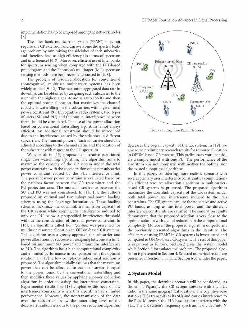
2 EURASIP Journal on Advances in Signal Processing
implementation has to be imposed among the network nodes[6].
The filter bank multicarrier system (FBMC) does notrequire any CP extension and can overcome the spectral leak-age problem by minimizing the sidelobes of each subcarrierand therefore lead to high efficiency (in terms of spectrumand interference) [6, 7]. Moreover, efficient use of filter banksfor spectrum sensing when compared with the FFT-basedpreiodogram and the Thomson’s multitaper (MT) spectrumsensing methods have been recently discussed in [6, 8].
The problem of resource allocation for conventional(noncognitive) multiuser multicarrier systems has beenwidely studied [9–12]. The maximum aggregated data rate indownlink can be obtained by assigning each subcarrier to theuser with the highest signal-to-noise ratio (SNR) and thenthe optimal power allocation that maximizes the channelcapacity is waterfilling on the subcarriers with a given totalpower constraint [9]. In cognitive radio systems, two typesof users (SU and PU) and the mutual interference betweenthem should be considered. The use of the power allocationbased on conventional waterfilling algorithm is not alwaysefficient. An additional constraint should be introduceddue to the interference caused by the sidelobes in differentsubcarriers. The transmit power of each subcarrier should beadjusted according to the channel status and the location ofthe subcarrier with respect to the PU spectrum.
Wang et al. in [13] proposed an iterative partitionedsingle user waterfilling algorithm. The algorithm aims tomaximize the capacity of the CR system under the totalpower constraint with the consideration of the per subcarrierpower constraint caused by the PUs interference limit.The per subcarrier power constraint is evaluated based onthe pathloss factor between the CR transmitter and thePU protection area. The mutual interference between theSU and PU was not considered. In [14, 15], the authorsproposed an optimal and two suboptimal power loadingschemes using the Lagrange formulation. These loadingschemes maximize the downlink transmission capacity ofthe CR system while keeping the interference induced toonly one PU below a prespecified interference thresholdwithout the consideration of the total power constraint. In[16], an algorithm called RC algorithm was presented formultiuser resource allocation in OFDM-based CR systems.This algorithm uses a greedy approach for subcarrier andpower allocations by successively assigning bits, one at a time,based on minimum SU power and minimum interferenceto PUs. The algorithm has a high computational complexityand a limited performance in comparison with the optimalsolution. In [17], a low complexity suboptimal solution isproposed. The algorithm initially assumes that the maximumpower that can be allocated to each subcarrier is equalto the power found by the conventional waterfilling andthen modifies these values by applying a power reductionalgorithm in order to satisfy the interference constraints.Experimental results like [18] emphasize the need of lowinterference constraints where this algorithm has a limitedperformance. Moreover, the nontransmission of the dataover the subcarriers below the waterfilling level or thedeactivated subcarriers due to the power reduction algorithm
Secondary user(SU1)
(SU2)
(SU3)(SU4)
Primary user(PU1)
(PU2)
(PU3)
(PU4)
Primary system basestation
CR base station(CBS)
Figure 1: Cognitive Radio Network.
decreases the overall capacity of the CR system. In [19], wegive some preliminary research results for resource allocationin OFDM-based CR systems. This preliminary work consid-ers a simple model with one PU. The performance of thealgorithm was not compared with neither the optimal northe existed suboptimal algorithms.
In this paper, considering more realistic scenario withseveral primary user interference constraints, a computation-ally efficient resource allocation algorithm in multicarrier-based CR systems is proposed. The proposed algorithmmaximizes the downlink capacity of the CR system underboth total power and interference induced to the PUsconstraints. The CR system can use the nonactive and activePU bands as long as the total power and the differentinterference constraints are satisfied. The simulation resultsdemonstrate that the proposed solution is very close to theoptimal solution with a good reduction in the computationalcomplexity. Moreover, the proposed algorithm outperformsthe previously presented algorithms in the literature. Theefficiency of using FBMC in CR systems is investigated andcompared to OFDM-based CR systems. The rest of this paperis organized as follows. Section 2 gives the system modelwhile Section 3 formulates the problem. The proposed algo-rithm is presented in Section 4. Selected numerical results arepresented in Section 5. Finally, Section 6 concludes the paper.
2. System Model
In this paper, the downlink scenario will be considered. Asshown in Figure 1, the CR system coexists with the PUsradio in the same geographical location. The cognitive basestation (CBS) transmits to its SUs and causes interference tothe PUs. Moreover, the PUs base station interferes with theSUs. The CR system’s frequency spectrum is divided into N
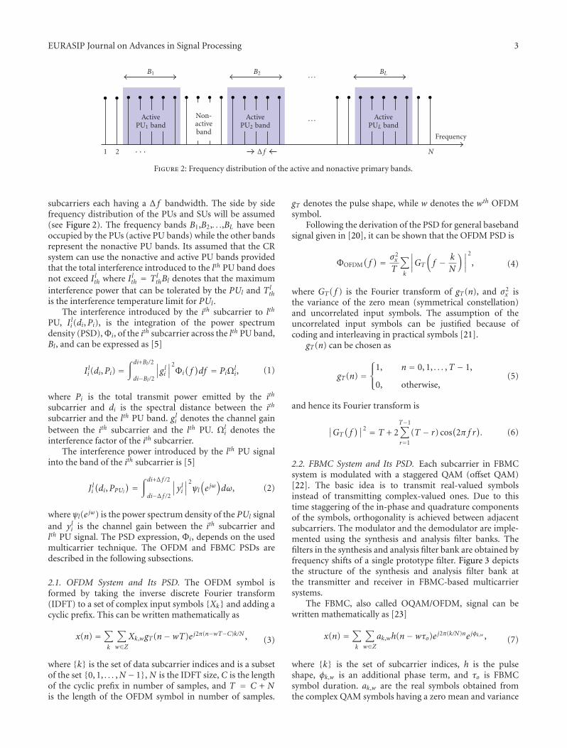
EURASIP Journal on Advances in Signal Processing 3
B1 B2 BL
ActivePU1 band
Non-activeband
ActivePU2 band
ActivePUL band
Frequency
1 2 Δ f N· · ·
. . .
. . .
Figure 2: Frequency distribution of the active and nonactive primary bands.
subcarriers each having a Δ f bandwidth. The side by sidefrequency distribution of the PUs and SUs will be assumed(see Figure 2). The frequency bands B1,B2,. . .,BL have beenoccupied by the PUs (active PU bands) while the other bandsrepresent the nonactive PU bands. Its assumed that the CRsystem can use the nonactive and active PU bands providedthat the total interference introduced to the lth PU band doesnot exceed Ilth where Ilth = Tl
thBl denotes that the maximuminterference power that can be tolerated by the PUl and Tl
this the interference temperature limit for PUl.
The interference introduced by the ith subcarrier to lth
PU, Ili (di,Pi), is the integration of the power spectrumdensity (PSD),Φi, of the ith subcarrier across the lth PU band,Bl, and can be expressed as [5]
Ili (di,Pi) =∫ di+Bl/2
di−Bl/2
∣∣∣gli∣∣∣
2Φi(f)df = PiΩ
li, (1)
where Pi is the total transmit power emitted by the ith
subcarrier and di is the spectral distance between the ith
subcarrier and the lth PU band. gli denotes the channel gainbetween the ith subcarrier and the lth PU. Ωl
i denotes theinterference factor of the ith subcarrier.
The interference power introduced by the lth PU signalinto the band of the ith subcarrier is [5]
J li(di,PPUl
) =∫ di+Δ f /2
di−Δ f /2
∣∣∣yli∣∣∣
2ψl(e jω)dω, (2)
where ψl(e jω) is the power spectrum density of the PUl signaland yli is the channel gain between the ith subcarrier andlth PU signal. The PSD expression, Φi, depends on the usedmulticarrier technique. The OFDM and FBMC PSDs aredescribed in the following subsections.
2.1. OFDM System and Its PSD. The OFDM symbol isformed by taking the inverse discrete Fourier transform(IDFT) to a set of complex input symbols {Xk} and adding acyclic prefix. This can be written mathematically as
x(n) =∑
k
∑
w∈ZXk,wgT(n−wT)e j2π(n−wT−C)k/N , (3)
where {k} is the set of data subcarrier indices and is a subsetof the set {0, 1, . . . ,N − 1}, N is the IDFT size, C is the lengthof the cyclic prefix in number of samples, and T = C + Nis the length of the OFDM symbol in number of samples.
gT denotes the pulse shape, while w denotes the wth OFDMsymbol.
Following the derivation of the PSD for general basebandsignal given in [20], it can be shown that the OFDM PSD is
ΦOFDM(f) = σ2
x
T
∑
k
∣∣∣∣GT
(f − k
N
)∣∣∣∣2
, (4)
where GT( f ) is the Fourier transform of gT(n), and σ2x is
the variance of the zero mean (symmetrical constellation)and uncorrelated input symbols. The assumption of theuncorrelated input symbols can be justified because ofcoding and interleaving in practical symbols [21].
gT(n) can be chosen as
gT(n) =⎧⎨⎩
1, n = 0, 1, . . . ,T − 1,
0, otherwise,(5)
and hence its Fourier transform is
∣∣GT(f)∣∣2 = T + 2
T−1∑
r=1
(T − r) cos(2π f r
). (6)
2.2. FBMC System and Its PSD. Each subcarrier in FBMCsystem is modulated with a staggered QAM (offset QAM)[22]. The basic idea is to transmit real-valued symbolsinstead of transmitting complex-valued ones. Due to thistime staggering of the in-phase and quadrature componentsof the symbols, orthogonality is achieved between adjacentsubcarriers. The modulator and the demodulator are imple-mented using the synthesis and analysis filter banks. Thefilters in the synthesis and analysis filter bank are obtained byfrequency shifts of a single prototype filter. Figure 3 depictsthe structure of the synthesis and analysis filter bank atthe transmitter and receiver in FBMC-based multicarriersystems.
The FBMC, also called OQAM/OFDM, signal can bewritten mathematically as [23]
x(n) =∑
k
∑
w∈Zak,wh(n−wτo)e j2π(k/N)ne jφk,w , (7)
where {k} is the set of subcarrier indices, h is the pulseshape, φk,w is an additional phase term, and τo is FBMCsymbol duration. ak,w are the real symbols obtained fromthe complex QAM symbols having a zero mean and variance
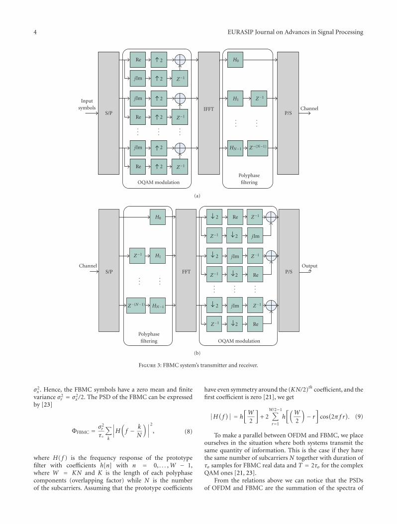
4 EURASIP Journal on Advances in Signal Processing
Inputsymbols Channel
Re
jIm
jIm
Re
2
2
2
2
2
2
jIm
Re
Z−1
Z−1
Z−1
OQAM modulation
IFFT
H0
H1
HN−1
Z−1
Z−(N−1)
P/SS/P
Polyphasefiltering
···
···
··· ··
·
···
(a)
ChannelS/P
H0
H1
HN−1
Z−1
Z−(N−1)
FFT
2
2
Z−1
2
2
Re Z−1
Z−1 jIm
jIm Z−1
Z−1 2 Re
jIm Z−1
2 Re
P/SOutput
Polyphasefiltering OQAM modulation
···
···
···
···
···
(b)
Figure 3: FBMC system’s transmitter and receiver.
σ2x . Hence, the FBMC symbols have a zero mean and finite
variance σ2r = σ2
x /2. The PSD of the FBMC can be expressedby [23]
ΦFBMC = σ2r
τ◦
∑
k
∣∣∣∣H(f − k
N
)∣∣∣∣2
, (8)
where H( f ) is the frequency response of the prototypefilter with coefficients h[n] with n = 0, . . . ,W − 1,where W = KN and K is the length of each polyphasecomponents (overlapping factor) while N is the numberof the subcarriers. Assuming that the prototype coefficients
have even symmetry around the (KN/2)th coefficient, and thefirst coefficient is zero [21], we get
∣∣H(f)∣∣ = h
[W
2
]+ 2
W/2−1∑
r=1
h[(
W
2
)− r
]cos
(2π f r
). (9)
To make a parallel between OFDM and FBMC, we placeourselves in the situation where both systems transmit thesame quantity of information. This is the case if they havethe same number of subcarriers N together with duration ofτo samples for FBMC real data and T = 2τo for the complexQAM ones [21, 23].
From the relations above we can notice that the PSDsof OFDM and FBMC are the summation of the spectra of
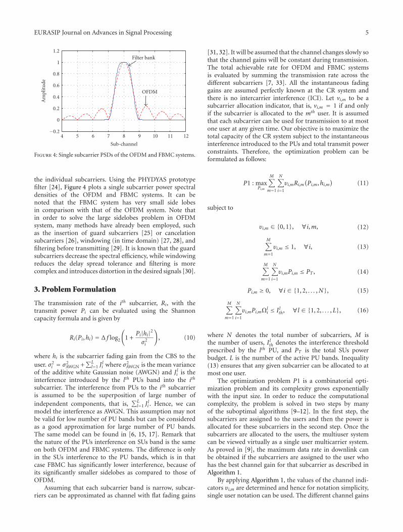
EURASIP Journal on Advances in Signal Processing 5
−0.2
0
0.2
0.4
0.6
0.8
1
1.2
4 5 6 7 8 9 10 11 12
Am
plit
ude
Filter bank
OFDM
Sub-channel
Figure 4: Single subcarrier PSDs of the OFDM and FBMC systems.
the individual subcarriers. Using the PHYDYAS prototypefilter [24], Figure 4 plots a single subcarrier power spectraldensities of the OFDM and FBMC systems. It can benoted that the FBMC system has very small side lobesin comparison with that of the OFDM system. Note thatin order to solve the large sidelobes problem in OFDMsystem, many methods have already been employed, suchas the insertion of guard subcarriers [25] or cancelationsubcarriers [26], windowing (in time domain) [27, 28], andfiltering before transmitting [29]. It is known that the guardsubcarriers decrease the spectral efficiency, while windowingreduces the delay spread tolerance and filtering is morecomplex and introduces distortion in the desired signals [30].
3. Problem Formulation
The transmission rate of the ith subcarrier, Ri, with thetransmit power Pi can be evaluated using the Shannoncapacity formula and is given by
Ri(Pi,hi) = Δ f log2
(1 +
Pi|hi|2σ2i
), (10)
where hi is the subcarrier fading gain from the CBS to theuser. σ2
i = σ2AWGN +
∑Ll=1 J
li where σ2
AWGN is the mean varianceof the additive white Gaussian noise (AWGN) and J li is theinterference introduced by the lth PUs band into the ith
subcarrier. The interference from PUs to the ith subcarrieris assumed to be the superposition of large number ofindependent components, that is,
∑Ll=1 J
li . Hence, we can
model the interference as AWGN. This assumption may notbe valid for low number of PU bands but can be consideredas a good approximation for large number of PU bands.The same model can be found in [6, 15, 17]. Remark thatthe nature of the PUs interference on SUs band is the sameon both OFDM and FBMC systems. The difference is onlyin the SUs interference to the PU bands, which is in thatcase FBMC has significantly lower interference, because ofits significantly smaller sidelobes as compared to those ofOFDM.
Assuming that each subcarrier band is narrow, subcar-riers can be approximated as channel with flat fading gains
[31, 32]. It will be assumed that the channel changes slowly sothat the channel gains will be constant during transmission.The total achievable rate for OFDM and FBMC systemsis evaluated by summing the transmission rate across thedifferent subcarriers [7, 33]. All the instantaneous fadinggains are assumed perfectly known at the CR system andthere is no intercarrier interference (ICI). Let vi,m to be asubcarrier allocation indicator, that is, vi,m = 1 if and onlyif the subcarrier is allocated to the mth user. It is assumedthat each subcarrier can be used for transmission to at mostone user at any given time. Our objective is to maximize thetotal capacity of the CR system subject to the instantaneousinterference introduced to the PUs and total transmit powerconstraints. Therefore, the optimization problem can beformulated as follows:
P1 : maxPi,m
M∑
m=1
N∑
i=1
υi,mRi,m(Pi,m,hi,m
)(11)
subject to
υi,m ∈ {0, 1}, ∀i,m, (12)
M∑
m=1
υi,m ≤ 1, ∀i, (13)
M∑
m=1
N∑
i=1
υi,mPi,m ≤ PT , (14)
Pi,m ≥ 0, ∀i ∈ {1, 2, . . . ,N}, (15)
M∑
m=1
N∑
i=1
υi,mPi,mΩli ≤ Ilth, ∀l ∈ {1, 2, . . . ,L}, (16)
where N denotes the total number of subcarriers, M isthe number of users, Ilth denotes the interference thresholdprescribed by the lth PU, and PT is the total SUs powerbudget. L is the number of the active PU bands. Inequality(13) ensures that any given subcarrier can be allocated to atmost one user.
The optimization problem P1 is a combinatorial opti-mization problem and its complexity grows exponentiallywith the input size. In order to reduce the computationalcomplexity, the problem is solved in two steps by manyof the suboptimal algorithms [9–12]. In the first step, thesubcarriers are assigned to the users and then the power isallocated for these subcarriers in the second step. Once thesubcarriers are allocated to the users, the multiuser systemcan be viewed virtually as a single user multicarrier system.As proved in [9], the maximum data rate in downlink canbe obtained if the subcarriers are assigned to the user whohas the best channel gain for that subcarrier as described inAlgorithm 1.
By applying Algorithm 1, the values of the channel indi-cators υi,m are determined and hence for notation simplicity,single user notation can be used. The different channel gains
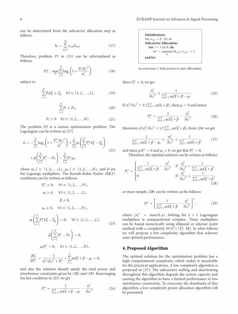
6 EURASIP Journal on Advances in Signal Processing
can be determined from the subcarrier allocation step asfollows:
hi =M∑
m=1
υi,mhi,m. (17)
Therefore, problem P1 in (11) can be reformulated asfollows:
P2 : maxPi
N∑
i=1
log2
(1 +
Pi|hi|2σ2i
)(18)
subject to
N∑
i=1
PiΩli ≤ Ilth ∀l ∈ {1, 2, . . . ,L}, (19)
N∑
i=1
Pi ≤ PT , (20)
Pi ≥ 0 ∀i ∈ {1, 2, . . . ,N}. (21)
The problem P2 is a convex optimization problem. TheLagrangian can be written as [17]
G = −N∑
i=1
log2
(1 +
P∗i |hi|2σ2i
)+
L∑
l=1
αl
⎛⎝
N∑
i=1
P∗i Ωli − Ilth
⎞⎠
+ β
⎛⎝
N∑
i=1
P∗i − PT⎞⎠−
N∑
i=1
P∗i μi,
(22)
where αl, l ∈ {1, 2, . . . ,L}, μi, i ∈ {1, 2, . . . ,N}, and β arethe Lagrange multipliers. The Karush-Kuhn-Tucker (KKT)conditions can be written as follows:
P∗i ≥ 0, ∀i ∈ {1, 2, . . . ,N},αl ≥ 0, ∀l ∈ {1, 2, . . . ,L},
β ≥ 0,
μi ≥ 0, ∀i ∈ {1, 2, . . . ,N},
αl
⎛⎝
N∑
i=1
P∗i Ωli − Ilth
⎞⎠ = 0, ∀l ∈ {1, 2, . . . ,L},
β
⎛⎝
N∑
i=1
P∗i − PT⎞⎠ = 0,
μiP∗i = 0, ∀i ∈ {1, 2, . . . ,N},
∂G
∂P∗i= −1
σ2i /|hi|2 + P∗i
+L∑
l=1
αlΩli + β − μi = 0,
(23)
and also the solution should satisfy the total power andinterference constraints given by (20) and (19). Rearrangingthe last condition in (23) we get
P∗i =1
∑Ll=1 αlΩ
li + β − μi
− σ2i
|hi|2. (24)
Initialization:Set υi,m = 0 ∀i,mSubcarrier Allocation:
for i = 1 to N dom∗ = argmax
m{hi,m}; υi,m∗ = 1
end for
Algorithm 1: Subcarriers to user allocation.
Since P∗i ≥ 0, we get
σ2i
|hi|2≤ 1∑L
l=1 αlΩli + β − μi
. (25)
If σ2i /|hi|2 < 1/(
∑Ll=1 αlΩi + β), then μi = 0 and hence
P∗i =1
∑Ll=1 αlΩ
li + β
− σ2i
|hi|2. (26)
Moreover, if σ2i /|hi|2 > 1/(
∑Ll=1 αlΩ
li + β), from (24) we get
1∑L
l=1 αlΩli + β − μi
≥ σ2i
|hi|2≥ 1∑L
l=1 αlΩli + β
, (27)
and since μiP∗i = 0 and μi ≥ 0, we get that P∗i = 0.Therefore, the optimal solution can be written as follows:
P∗i =
⎧⎪⎪⎪⎪⎨⎪⎪⎪⎪⎩
1∑L
l=1 αlΩli + β
− σ2i
|hi|2if
σ2i
|hi|2<
1∑L
l=1 αlΩli + β
,
0 ifσ2i
|hi|2≥ 1∑L
l=1 αlΩli + β
,
(28)
or more simply, (28) can be written as the follows:
P∗i =[
1∑L
l=1 αlΩli + β
− σ2i
|hi|2]+
, (29)
where [x]+ = max(0, x). Solving for L + 1 Lagrangianmultipliers is computational complex. These multiplierscan be found numerically using ellipsoid or interior pointmethod with a complexity O(N3) [17, 34]. In what followswe will propose a low complexity algorithm that achievesnear optimal performance.
4. Proposed Algorithm
The optimal solution for the optimization problem has ahigh computational complexity which makes it unsuitablefor the practical applications. A low complexity algorithm isproposed in [17]. The subcarriers nulling and deactivatingthroughout this algorithm degrade the system capacity andcausing the algorithm to have a limited performance in lowinterference constraints. To overcome the drawbacks of thisalgorithm, a low complexity power allocation algorithm willbe presented.
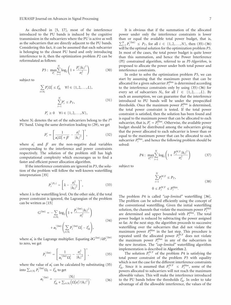
EURASIP Journal on Advances in Signal Processing 7
As described in [5, 17], most of the interferenceintroduced to the PU bands is induced by the cognitivetransmission in the subcarriers where the PU is active as wellas the subcarriers that are directly adjacent to the PU bands.Considering this fact, it can be assumed that each subcarrieris belonging to the closest PU band and only introducinginterference to it, then the optimization problem P2 can bereformulated as follows:
P3 : maxP′i
N∑
i=1
log2
(1 +
P′i |hi|2σ2i
)(30)
subject to∑
i∈Nl
P′iΩli ≤ Ilth ∀l ∈ {1, 2, . . . ,L},
N∑
i=1
P′i ≤ PT ,
P′i ≥ 0 ∀i ∈ {1, 2, . . . ,N},
(31)
where Nl denotes the set of the subcarriers belong to the lth
PU band. Using the same derivation leading to (29), we get
P′i =[
1
α′lΩli + β′
− σ2i
|hi|2]+
, (32)
where α′l and β′ are the non-negative dual variablescorresponding to the interference and power constraintsrespectively. The solution of the problem still has highcomputational complexity which encourages us to find afaster and efficient power allocation algorithm.
If the interference constraints are ignored in P3, the solu-tion of the problem will follow the well-known waterfillinginterpretation [35]
P′(PT )i =
[λ− σ2
i
|hi|2]+
, (33)
where λ is the waterfilling level. On the other side, if the totalpower constraint is ignored, the Lagrangian of the problemcan be written as [15]
G(Int) = −∑
i∈Nl
log2
(1 +
P′(Int)i |hi|2σ2i
)
+ α′(Int)l
⎛⎝∑
i∈Nl
P′(Int)i Ωl
i − Ilth
⎞⎠,
(34)
where α′l is the Lagrange multiplier. Equating ∂G(Int)/∂P′(Int)i
to zero, we get
P′(Int)i =
⎡⎣ 1
α′(Int)l Ωl
i
− σ2i
|hi|2
⎤⎦
+
, (35)
where the value of α′l can be calculated by substituting (35)
into∑
i∈NlP′(Int)i Ωi = Ilth to get
α′(Int)l = |Nl|
Ilth +∑
i∈Nl
(Ωliσ
2i /|hi|2
) . (36)
It is obvious that if the summation of the allocatedpower under only the interference constraints is lowerthan or equal the available total power budget, that is,∑N
i=1 P′(Int)i ≤ PT , for all i ∈ {1, 2, . . . ,N}, then (35)-(36)
will be the optimal solution for the optimization problem P3.In most of the cases, the total power budget is quite lowerthan this summation, and hence the Power Interference(PI) constrained algorithm, referred to as PI-Algorithm, isproposed to allocate the power under both total power andinterference constraints.
In order to solve the optimization problem P3, we canstart by assuming that the maximum power that can beallocated for a given subcarrier PMax
i is determined accordingto the interference constraints only by using (35)-(36) forevery set of subcarriers Nl, for all l ∈ {1, 2, . . . ,L}. Bysuch an assumption, we can guarantee that the interferenceintroduced to PU bands will be under the prespecifiedthresholds. Once the maximum power PMax
i is determined,the total power constraint is tested. If the total powerconstraint is satisfied, then the solution has been found andis equal to the maximum power that can be allocated to eachsubcarrier, that is, P′i = PMax
i . Otherwise, the available powerbudget should be distributed among the subcarriers givingthat the power allocated to each subcarrier is lower than orequal to the maximum power that can be allocated to eachsubcarrier PMax
i , and hence the following problem should besolved:
P4 : maxPW.Fi
N∑
i=1
log2
(1 +
PW.Fi |hi|2σ2i
)(37)
subject to
N∑
i=1
PW.Fi ≤ PT ,
0 ≤ PW.Fi ≤ PMax
i .
(38)
The problem P4 is called “cap-limited” waterfilling [36].The problem can be solved efficiently using the concept ofthe conventional waterfilling. Given the initial waterfillingsolution, the channels that violate the maximum power PMax
i
are determined and upper bounded with PMaxi . The total
power budget is reduced by subtracting the power assignedso far. At the next step, the algorithm proceeds to successivewaterfilling over the subcarriers that did not violate themaximum power PMax
i in the last step. This procedure isrepeated until the allocated power PW.F
i does not violatethe maximum power PMax
i in any of the subcarriers inthe new iteration. The “cap-limited” waterfilling algorithmimplementation is described in Algorithm 2.
The solution PW.Fi of the problem P4 is satisfying the
total power constraint of the problem P3 with equalitywhich is not the case for the different interference constraintsIlth. Since it is assumed that PW.F
i ≤ PMaxi , some of the
powers allocated to subcarriers will not reach the maximumallowable values. This will make the interference introducedto the PU bands below the thresholds Ilth. In order to takeadvantage of all the allowable interference, the values of the
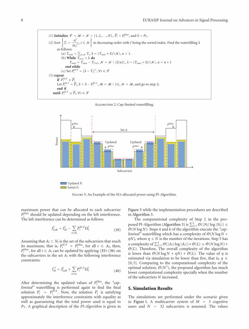
8 EURASIP Journal on Advances in Signal Processing
(1) Initialize F =M = N = {1, 2, . . . ,N}, Pi = PMaxi , and S = PT .
(2) Sort
{Ti = σ2
i
|hi|2, i ∈ N
}in decreasing order with J being the sorted index. Find the waterfilling λ
as follows:(a) Tsum =
∑i∈N Ti, λ = (Tsum + S)/|N |, n = 1.
(b) While TJ(n) > λ doTsum = Tsum − TJ(n), N = N \ {J(n)}, λ = (Tsum + S)/|N |, n = n + 1
end while(c) Set PW.F
i = [λ− Ti]+,∀i ∈ F(3) repeat
if PW.Fi ≥ Pi
Let PW.Fi = Pi, S = S− PW.F
i , M =M \ {i}, N =M, and go to step 2;end if
until PW.Fi ≤ Pi,∀i ∈ F
Algorithm 2: Cap-limited waterfilling.
Initial Pi
Updated Pi
Pow
er
Subcarriers
PMax
Set A
PMax
Updated
PMax
Updated
PMax
Figure 5: An Example of the SUs allocated power using PI-Algorithm.
maximum power that can be allocated to each subcarrierPMaxi should be updated depending on the left interference.
The left interference can be determined as follows:
IlLeft = Ilth −∑
i∈Nl
PW.Fi Ωl
i. (39)
Assuming that Al ⊂ Nl is the set of the subcarriers that reachits maximum, that is, PW.F
i = PMaxi , for all i ∈ Al, then,
PMaxi , for all i ∈ Al can be updated by applying (35)-(36) on
the subcarriers in the set Al with the following interferenceconstraints:
I′lth = IlLeft +
∑
i∈AlPW.Fi Ωl
i. (40)
After determining the updated values of PMaxi , the “cap-
limited” waterfilling is performed again to find the finalsolution P′i = PW.F
i . Now, the solution P′i is satisfyingapproximately the interference constraints with equality aswell as guaranteing that the total power used is equal toPT . A graphical description of the PI-Algorithm is given in
Figure 5 while the implementation procedures are describedin Algorithm 3.
The computational complexity of Step 2 in the pro-posed PI-Algorithm (Algorithm 3) is
∑Ll=1 O(|Nl| log |Nl|) ≤
O(N logN). Steps 4 and 6 of the algorithm execute the “cap-limited” waterfilling which has a complexity of O(N logN +ηN), where η ≤ N is the number of the iterations. Step 5 hasa complexity of
∑Ll=1 O(|Al| log |Al|) +O(L) ≤ O(N logN) +
O(L). Therefore, The overall complexity of the algorithmis lower than O(N logN + ηN) + O(L). The value of η isestimated via simulation to be lower than five, that is, η ∈[0, 5]. Comparing to the computational complexity of theoptimal solution, O(N3), the proposed algorithm has muchlower computational complexity specially when the numberof the subcarriers N increased.
5. Simulation Results
The simulations are performed under the scenario givenin Figure 1. A multicarrier system of M = 3 cognitiveusers and N = 32 subcarriers is assumed. The values
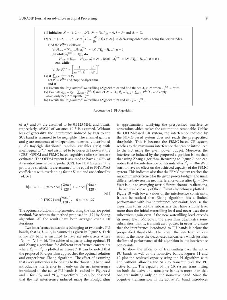
EURASIP Journal on Advances in Signal Processing 9
(1) Initialize N = {1, 2, · · · ,N}, Nl = Nl , I lLeft = 0, S = PT and Al = ∅.
(2)∀l ∈ {1, 2, · · · ,L}, sort
{Hi = σ2
i
|hi|2Ωli, i ∈ Nl
}in decreasing order with k being the sorted index.
Find the PMaxi as follows:
(a) Hsum =∑
i∈NlHi, α
′(Int)l = |Nl|/(I lth +Hsum), n = 1.
(b) while α′(Int)l > H−1
k(n) do
Hsum = Hsum −Hk(n), Nl = Nl \ {k(n)}, α′(Int)l = |Nl|/(I lth +Hsum), n = n + 1
end while
(c) Set PMaxi =
[1
α′(Int)l Ωl
i
− σ2i
|hi|2]+
(3) if∑
i∈N PMaxi ≤ PT
Let P′i = PMaxi and stop the algorithm.
end if(4) Execute the “cap-limited” waterfilling (Algorithm 2) and find the set Al ⊂ Nl where PW.F
i = PMaxi .
(5) Evaluate I lLeft = I lth −∑
i∈Nl PW.Fi Ωl
i and set Nl =Al, I lth = I lLeft +∑
i∈AlPW.Fi Ωl
i and applyagain only step 2 to update PMax
i .(6) Execute the “cap-limited” waterfilling (Algorithm 2) and set P′i = PW.F
i .
Algorithm 3: PI-Algorithm.
of Δ f and PT are assumed to be 0.3125 MHz and 1 watt,respectively. AWGN of variance 10−6 is assumed. Withoutloss of generality, the interference induced by PUs to theSUs band is assumed to be negligible. The channel gains hand g are outcomes of independent, identically distributed(i.i.d) Rayleigh distributed random variables (rv’s) withmean equal to “1” and assumed to be perfectly known at the(CBS). OFDM and FBMC-based cognitive radio systems areevaluated. The OFDM system is assumed to have a 6.67% ofits symbol time as cyclic prefix (CP). For FBMC system, theprototype coefficients are assumed to be equal to PHYDYAScoefficients with overlapping factor K = 4 and are defined by[24, 37]
h[n] = 1− 1.94392 cos(
2πn128
)+√
2 cos(
4πn128
)
− 0.470294 cos(
6πn128
), 0 ≤ n ≤ 127,
(41)
The optimal solution is implemented using the interior pointmethod. We refer to the method proposed in [17] by Zhangalgorithm. All the results have been averaged over 1000iterations.
Two interference constraints belonging to two active PUbands, that is, L = 2, is assumed as given in Figure 6. Eachactive PU band is assumed to have six subcarriers where|N1| = |N2| = 16. The achieved capacity using optimal, PIand Zhang algorithms for different interference constraintswhere I1
th = I2th is plotted in Figure 7. It can be noted that
the proposed PI-algorithm approaches the optimal solutionand outperforms Zhang algorithm. The effect of assumingthat every subcarrier is belonging to the closest PU band andintroducing interference to it only on the net interferenceintroduced to the active PU bands is studied in Figures 8and 9 for PU1 and PU2, respectively. It can be observedthat the net interference induced using the PI-algorithm
is approximately satisfying the prespecified interferenceconstraints which makes the assumption reasonable. Unlikethe OFDM-based CR system, the interference induced bythe FBMC-based system does not reach the pre-specifiedthresholds. This is because the FBMC-based CR systemreaches to the maximum interference that can be introducedto the PU using the given power budget. Moreover, theinterference induced by the proposed algorithm is less thanthat using Zhang algorithm. Returning to Figure 7, one cannotice that the interference constraints after Ilth = 10mWattstart to have no effect on the achieved capacity of the FBMCsystem. This indicates also that the FBMC system reaches themaximum interference for the given power budget. The smalldifference between the net interference values after Ilth = 10mWatt is due to averaging over different channel realizations.The achieved capacity of the different algorithms is plotted inFigure 10 with lower values of the interference constraints.It can be noticed that Zhang algorithm has a limitedperformance with low interference constraints because thealgorithm turns off the subcarriers that have a noise levelmore than the initial waterfilling level and never uses thesesubcarriers again even if the new waterfilling level exceedsits noise level. Moreover, the algorithm deactivates somesubcarriers, that is, transmit zero power, in order to ensurethat the interference introduced to PU bands is below theprespecified thresholds. The lower the interference con-straints, the more the deactivated subcarriers which justifiesthe limited performance of this algorithm in low interferenceconstraints.
To show the efficiency of transmitting over the activePU bands as well as the nonactive bands, Figures 11 and12 plot the achieved capacity using the PI algorithm withand without allowing the SUs to transmit over the PUactive bands. The capacity of the CR system transmittingon both the active and nonactive bands is more than thatone transmitting only on the nonactive band. Since thecognitive transmission in the active PU band introduces
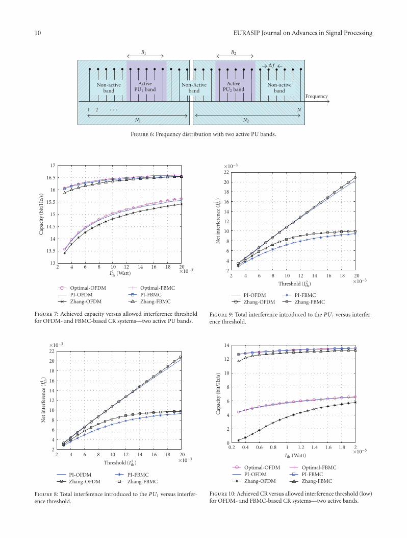
10 EURASIP Journal on Advances in Signal Processing
Non-activeband
ActivePU1 band
Non-Activeband
ActivePU2 band
Non-activeband
B1 B2
N1 N2
N1 2
Frequency
· · ·
Δ f
Figure 6: Frequency distribution with two active PU bands.
13
13.5
14
14.5
15
15.5
16
16.5
17
Optimal-OFDMPI-OFDMZhang-OFDM
Optimal-FBMCPI-FBMCZhang-FBMC
I1th (Watt)
Cap
acit
y(b
it/H
z/s)
2 4 6 8 10 12 14 16 18 20×10−3
Figure 7: Achieved capacity versus allowed interference thresholdfor OFDM- and FBMC-based CR systems—two active PU bands.
2 4 6 8 10 12 14 16 18 20×10−3
2
4
6
8
10
12
14
16
18
20
22×10−3
Net
inte
rfer
ence
(I1 th
)
Threshold (I1th)
PI-OFDMZhang-OFDM
PI-FBMCZhang-FBMC
Figure 8: Total interference introduced to the PU1 versus interfer-ence threshold.
2 4 6 8 10 12 14 16 18 20×10−3
2
4
6
8
10
12
14
16
18
20
22×10−3
Net
inte
rfer
ence
(I2 th
)
Threshold (I2th)
PI-OFDMZhang-OFDM
PI-FBMCZhang-FBMC
Figure 9: Total interference introduced to the PU2 versus interfer-ence threshold.
0.2 0.4 0.6 0.8 1 1.2 1.4 1.6 1.8 2×10⁻⁵
0
2
4
6
8
10
12
14
Cap
acit
y(b
it/H
z/s)
Ith (Watt)
Optimal-OFDMPI-OFDMZhang-OFDM
Optimal-FBMCPI-FBMCZhang-FBMC
Figure 10: Achieved CR versus allowed interference threshold (low)for OFDM- and FBMC-based CR systems—two active bands.
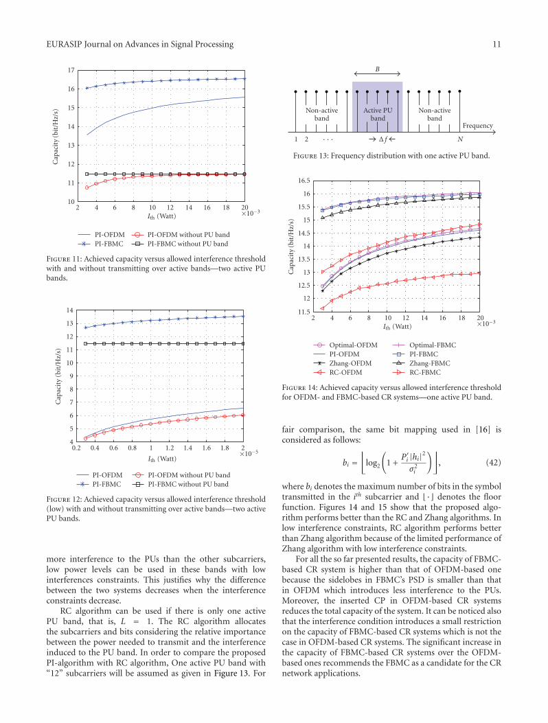
EURASIP Journal on Advances in Signal Processing 11
10
11
12
13
14
15
16
17
2 4 6 8 10 12 14 16 18 20×10−3
Ith (Watt)
Cap
acit
y(b
it/H
z/s)
PI-OFDM PI-OFDM without PU bandPI-FBMC PI-FBMC without PU band
Figure 11: Achieved capacity versus allowed interference thresholdwith and without transmitting over active bands—two active PUbands.
0.2 0.4 0.6 0.8 1 1.2 1.4 1.6 1.8 2×10⁻⁵
4
5
6
7
8
9
10
11
12
13
14
Cap
acit
y(b
it/H
z/s)
Ith (Watt)
PI-OFDM PI-OFDM without PU bandPI-FBMC PI-FBMC without PU band
Figure 12: Achieved capacity versus allowed interference threshold(low) with and without transmitting over active bands—two activePU bands.
more interference to the PUs than the other subcarriers,low power levels can be used in these bands with lowinterferences constraints. This justifies why the differencebetween the two systems decreases when the interferenceconstraints decrease.
RC algorithm can be used if there is only one activePU band, that is, L = 1. The RC algorithm allocatesthe subcarriers and bits considering the relative importancebetween the power needed to transmit and the interferenceinduced to the PU band. In order to compare the proposedPI-algorithm with RC algorithm, One active PU band with“12” subcarriers will be assumed as given in Figure 13. For
Non-activeband
Active PUband
Non-activeband
B
1 2 Δ f N
Frequency
· · ·
Figure 13: Frequency distribution with one active PU band.
11.5
12
12.5
13
13.5
14
14.5
15
15.5
16
16.5
2 4 6 8 10 12 14 16 18 20×10−3
Ith (Watt)
Cap
acit
y(b
it/H
z/s)
Optimal-OFDMPI-OFDMZhang-OFDMRC-OFDM
Optimal-FBMCPI-FBMCZhang-FBMCRC-FBMC
Figure 14: Achieved capacity versus allowed interference thresholdfor OFDM- and FBMC-based CR systems—one active PU band.
fair comparison, the same bit mapping used in [16] isconsidered as follows:
bi =⌊
log2
(1 +
P′i |hi|2σ2i
)⌋, (42)
where bi denotes the maximum number of bits in the symboltransmitted in the ith subcarrier and �· denotes the floorfunction. Figures 14 and 15 show that the proposed algo-rithm performs better than the RC and Zhang algorithms. Inlow interference constraints, RC algorithm performs betterthan Zhang algorithm because of the limited performance ofZhang algorithm with low interference constraints.
For all the so far presented results, the capacity of FBMC-based CR system is higher than that of OFDM-based onebecause the sidelobes in FBMC’s PSD is smaller than thatin OFDM which introduces less interference to the PUs.Moreover, the inserted CP in OFDM-based CR systemsreduces the total capacity of the system. It can be noticed alsothat the interference condition introduces a small restrictionon the capacity of FBMC-based CR systems which is not thecase in OFDM-based CR systems. The significant increase inthe capacity of FBMC-based CR systems over the OFDM-based ones recommends the FBMC as a candidate for the CRnetwork applications.
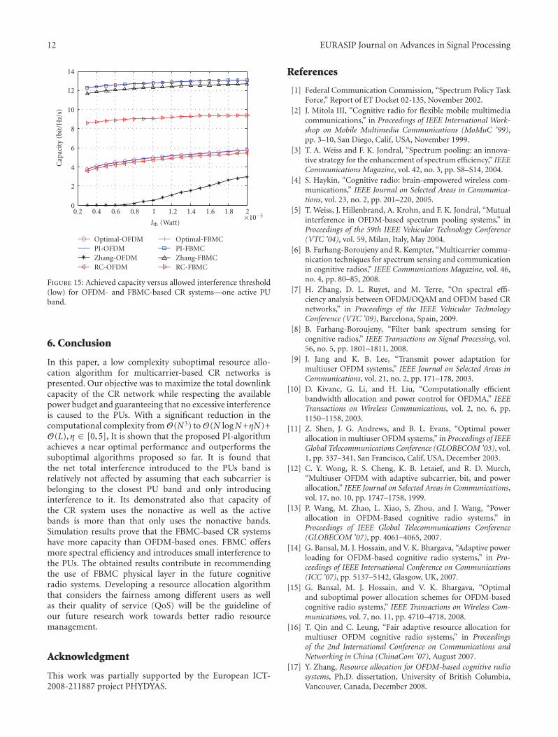
12 EURASIP Journal on Advances in Signal Processing
0.2 0.4 0.6 0.8 1 1.2 1.4 1.6 1.8 2×10⁻⁵
0
2
4
6
8
10
12
14
Cap
acit
y(b
it/H
z/s)
Ith (Watt)
Optimal-OFDMPI-OFDMZhang-OFDMRC-OFDM
Optimal-FBMCPI-FBMCZhang-FBMCRC-FBMC
Figure 15: Achieved capacity versus allowed interference threshold(low) for OFDM- and FBMC-based CR systems—one active PUband.
6. Conclusion
In this paper, a low complexity suboptimal resource allo-cation algorithm for multicarrier-based CR networks ispresented. Our objective was to maximize the total downlinkcapacity of the CR network while respecting the availablepower budget and guaranteeing that no excessive interferenceis caused to the PUs. With a significant reduction in thecomputational complexity from O(N3) to O(N logN+ηN)+O(L),η ∈ [0, 5], It is shown that the proposed PI-algorithmachieves a near optimal performance and outperforms thesuboptimal algorithms proposed so far. It is found thatthe net total interference introduced to the PUs band isrelatively not affected by assuming that each subcarrier isbelonging to the closest PU band and only introducinginterference to it. Its demonstrated also that capacity ofthe CR system uses the nonactive as well as the activebands is more than that only uses the nonactive bands.Simulation results prove that the FBMC-based CR systemshave more capacity than OFDM-based ones. FBMC offersmore spectral efficiency and introduces small interference tothe PUs. The obtained results contribute in recommendingthe use of FBMC physical layer in the future cognitiveradio systems. Developing a resource allocation algorithmthat considers the fairness among different users as wellas their quality of service (QoS) will be the guideline ofour future research work towards better radio resourcemanagement.
Acknowledgment
This work was partially supported by the European ICT-2008-211887 project PHYDYAS.
References
[1] Federal Communication Commission, “Spectrum Policy TaskForce,” Report of ET Docket 02-135, November 2002.
[2] J. Mitola III, “Cognitive radio for flexible mobile multimediacommunications,” in Proceedings of IEEE International Work-shop on Mobile Multimedia Communications (MoMuC ’99),pp. 3–10, San Diego, Calif, USA, November 1999.
[3] T. A. Weiss and F. K. Jondral, “Spectrum pooling: an innova-tive strategy for the enhancement of spectrum efficiency,” IEEECommunications Magazine, vol. 42, no. 3, pp. S8–S14, 2004.
[4] S. Haykin, “Cognitive radio: brain-empowered wireless com-munications,” IEEE Journal on Selected Areas in Communica-tions, vol. 23, no. 2, pp. 201–220, 2005.
[5] T. Weiss, J. Hillenbrand, A. Krohn, and F. K. Jondral, “Mutualinterference in OFDM-based spectrum pooling systems,” inProceedings of the 59th IEEE Vehicular Technology Conference(VTC ’04), vol. 59, Milan, Italy, May 2004.
[6] B. Farhang-Boroujeny and R. Kempter, “Multicarrier commu-nication techniques for spectrum sensing and communicationin cognitive radios,” IEEE Communications Magazine, vol. 46,no. 4, pp. 80–85, 2008.
[7] H. Zhang, D. L. Ruyet, and M. Terre, “On spectral effi-ciency analysis between OFDM/OQAM and OFDM based CRnetworks,” in Proceedings of the IEEE Vehicular TechnologyConference (VTC ’09), Barcelona, Spain, 2009.
[8] B. Farhang-Boroujeny, “Filter bank spectrum sensing forcognitive radios,” IEEE Transactions on Signal Processing, vol.56, no. 5, pp. 1801–1811, 2008.
[9] J. Jang and K. B. Lee, “Transmit power adaptation formultiuser OFDM systems,” IEEE Journal on Selected Areas inCommunications, vol. 21, no. 2, pp. 171–178, 2003.
[10] D. Kivanc, G. Li, and H. Liu, “Computationally efficientbandwidth allocation and power control for OFDMA,” IEEETransactions on Wireless Communications, vol. 2, no. 6, pp.1150–1158, 2003.
[11] Z. Shen, J. G. Andrews, and B. L. Evans, “Optimal powerallocation in multiuser OFDM systems,” in Proceedings of IEEEGlobal Telecommunications Conference (GLOBECOM ’03), vol.1, pp. 337–341, San Francisco, Calif, USA, December 2003.
[12] C. Y. Wong, R. S. Cheng, K. B. Letaief, and R. D. Murch,“Multiuser OFDM with adaptive subcarrier, bit, and powerallocation,” IEEE Journal on Selected Areas in Communications,vol. 17, no. 10, pp. 1747–1758, 1999.
[13] P. Wang, M. Zhao, L. Xiao, S. Zhou, and J. Wang, “Powerallocation in OFDM-Based cognitive radio systems,” inProceedings of IEEE Global Telecommunications Conference(GLOBECOM ’07), pp. 4061–4065, 2007.
[14] G. Bansal, M. J. Hossain, and V. K. Bhargava, “Adaptive powerloading for OFDM-based cognitive radio systems,” in Pro-ceedings of IEEE International Conference on Communications(ICC ’07), pp. 5137–5142, Glasgow, UK, 2007.
[15] G. Bansal, M. J. Hossain, and V. K. Bhargava, “Optimaland suboptimal power allocation schemes for OFDM-basedcognitive radio systems,” IEEE Transactions on Wireless Com-munications, vol. 7, no. 11, pp. 4710–4718, 2008.
[16] T. Qin and C. Leung, “Fair adaptive resource allocation formultiuser OFDM cognitive radio systems,” in Proceedingsof the 2nd International Conference on Communications andNetworking in China (ChinaCom ’07), August 2007.
[17] Y. Zhang, Resource allocation for OFDM-based cognitive radiosystems, Ph.D. dissertation, University of British Columbia,Vancouver, Canada, December 2008.
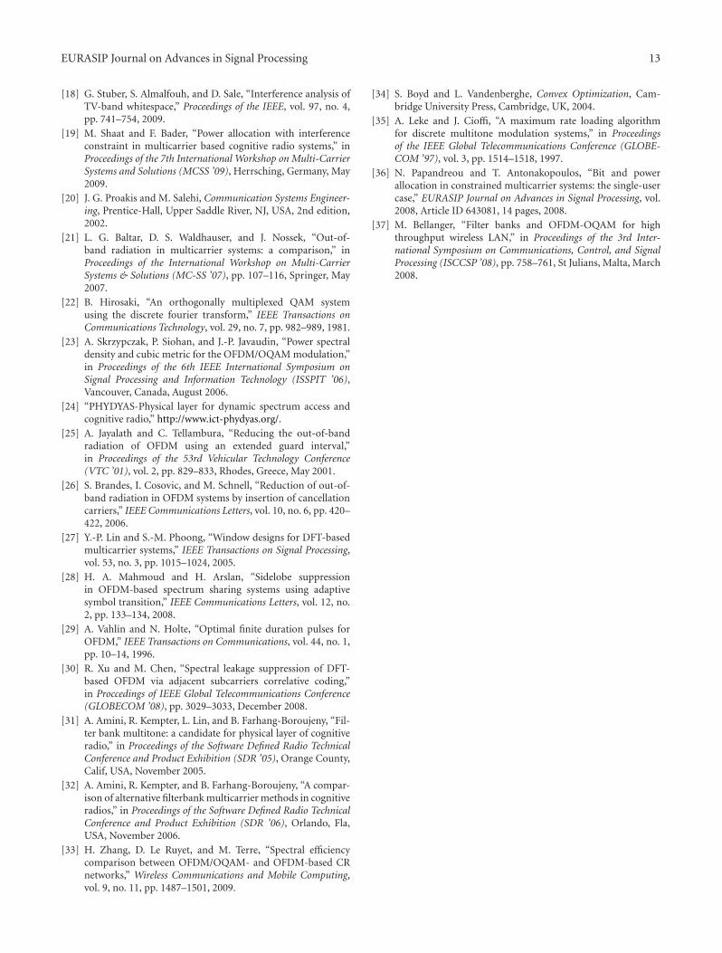
EURASIP Journal on Advances in Signal Processing 13
[18] G. Stuber, S. Almalfouh, and D. Sale, “Interference analysis ofTV-band whitespace,” Proceedings of the IEEE, vol. 97, no. 4,pp. 741–754, 2009.
[19] M. Shaat and F. Bader, “Power allocation with interferenceconstraint in multicarrier based cognitive radio systems,” inProceedings of the 7th International Workshop on Multi-CarrierSystems and Solutions (MCSS ’09), Herrsching, Germany, May2009.
[20] J. G. Proakis and M. Salehi, Communication Systems Engineer-ing, Prentice-Hall, Upper Saddle River, NJ, USA, 2nd edition,2002.
[21] L. G. Baltar, D. S. Waldhauser, and J. Nossek, “Out-of-band radiation in multicarrier systems: a comparison,” inProceedings of the International Workshop on Multi-CarrierSystems & Solutions (MC-SS ’07), pp. 107–116, Springer, May2007.
[22] B. Hirosaki, “An orthogonally multiplexed QAM systemusing the discrete fourier transform,” IEEE Transactions onCommunications Technology, vol. 29, no. 7, pp. 982–989, 1981.
[23] A. Skrzypczak, P. Siohan, and J.-P. Javaudin, “Power spectraldensity and cubic metric for the OFDM/OQAM modulation,”in Proceedings of the 6th IEEE International Symposium onSignal Processing and Information Technology (ISSPIT ’06),Vancouver, Canada, August 2006.
[24] “PHYDYAS-Physical layer for dynamic spectrum access andcognitive radio,” http://www.ict-phydyas.org/.
[25] A. Jayalath and C. Tellambura, “Reducing the out-of-bandradiation of OFDM using an extended guard interval,”in Proceedings of the 53rd Vehicular Technology Conference(VTC ’01), vol. 2, pp. 829–833, Rhodes, Greece, May 2001.
[26] S. Brandes, I. Cosovic, and M. Schnell, “Reduction of out-of-band radiation in OFDM systems by insertion of cancellationcarriers,” IEEE Communications Letters, vol. 10, no. 6, pp. 420–422, 2006.
[27] Y.-P. Lin and S.-M. Phoong, “Window designs for DFT-basedmulticarrier systems,” IEEE Transactions on Signal Processing,vol. 53, no. 3, pp. 1015–1024, 2005.
[28] H. A. Mahmoud and H. Arslan, “Sidelobe suppressionin OFDM-based spectrum sharing systems using adaptivesymbol transition,” IEEE Communications Letters, vol. 12, no.2, pp. 133–134, 2008.
[29] A. Vahlin and N. Holte, “Optimal finite duration pulses forOFDM,” IEEE Transactions on Communications, vol. 44, no. 1,pp. 10–14, 1996.
[30] R. Xu and M. Chen, “Spectral leakage suppression of DFT-based OFDM via adjacent subcarriers correlative coding,”in Proccedings of IEEE Global Telecommunications Conference(GLOBECOM ’08), pp. 3029–3033, December 2008.
[31] A. Amini, R. Kempter, L. Lin, and B. Farhang-Boroujeny, “Fil-ter bank multitone: a candidate for physical layer of cognitiveradio,” in Proceedings of the Software Defined Radio TechnicalConference and Product Exhibition (SDR ’05), Orange County,Calif, USA, November 2005.
[32] A. Amini, R. Kempter, and B. Farhang-Boroujeny, “A compar-ison of alternative filterbank multicarrier methods in cognitiveradios,” in Proceedings of the Software Defined Radio TechnicalConference and Product Exhibition (SDR ’06), Orlando, Fla,USA, November 2006.
[33] H. Zhang, D. Le Ruyet, and M. Terre, “Spectral efficiencycomparison between OFDM/OQAM- and OFDM-based CRnetworks,” Wireless Communications and Mobile Computing,vol. 9, no. 11, pp. 1487–1501, 2009.
[34] S. Boyd and L. Vandenberghe, Convex Optimization, Cam-bridge University Press, Cambridge, UK, 2004.
[35] A. Leke and J. Cioffi, “A maximum rate loading algorithmfor discrete multitone modulation systems,” in Proceedingsof the IEEE Global Telecommunications Conference (GLOBE-COM ’97), vol. 3, pp. 1514–1518, 1997.
[36] N. Papandreou and T. Antonakopoulos, “Bit and powerallocation in constrained multicarrier systems: the single-usercase,” EURASIP Journal on Advances in Signal Processing, vol.2008, Article ID 643081, 14 pages, 2008.
[37] M. Bellanger, “Filter banks and OFDM-OQAM for highthroughput wireless LAN,” in Proceedings of the 3rd Inter-national Symposium on Communications, Control, and SignalProcessing (ISCCSP ’08), pp. 758–761, St Julians, Malta, March2008.
Hindawi Publishing CorporationEURASIP Journal on Advances in Signal ProcessingVolume 2010, Article ID 307983, 13 pagesdoi:10.1155/2010/307983
Research Article
Packet Format Design and Decision Directed Tracking Methodsfor Filter Bank Multicarrier Systems
Peiman Amini and Behrouz Farhang-Boroujeny
The Electrical and Computer Engineering Department, University of Utah, UT 84112, USA
Correspondence should be addressed to Behrouz Farhang-Boroujeny, [email protected]
Received 11 May 2009; Revised 29 September 2009; Accepted 28 December 2009
Academic Editor: Pierre Siohan
Copyright © 2010 P. Amini and B. Farhang-Boroujeny. This is an open access article distributed under the Creative CommonsAttribution License, which permits unrestricted use, distribution, and reproduction in any medium, provided the original work isproperly cited.
Packetized data transmission is commonly used in wireless communication systems. Each packet starts with a preamble which isused to synchronize the receiver with carrier frequency of the incoming signal, to find a good timing phase, and to identify thechannel impulse response or to adjust a set of channel equalizer parameters. In this paper, following the same philosophy, wedevelop a packet format for multicarrier systems that operate based on filter banks, filter bank multicarrier (FBMC) systems. Therelated algorithms for carrier frequency and timing recovery as well as channel identification/equalizer adjustment and methods forcarrier and timing tracking loops are proposed. The proposed ideas are evaluated and their satisfactory performance are presentedthrough computer simulations.
1. Introduction
Multicarrier modulation has been recognized as the mostpromising approach for practical and efficient realization ofbroadband communication systems. Among various multi-carrier modulation methods, orthogonal frequency divisionmultiplexing (OFDM), [1], is the most widely adoptedmethod in the current standards. While OFDM may be agood choice for point-to-point communication, it may notbe the best choice in many other applications. For instance,in the up-link of an orthogonal frequency division multipleaccess (OFDMA) network, the loss of synchronizationbetween the carriers of different nodes will result in asignificant performance loss and often complex processingsteps have to be adopted at the base station to recover this loss(partially); see [2] and the references therein. Such complexprocessing can be avoided by adopting alternative methodsthat use filter banks for multicarrier modulation. OFDMAlimitation is the result of the fact that the side-lobes (equiv-alent to stopband) of the filters based on which OFDMAsignals are constructed are relatively large. In filter bankmulticarrier (FBMC) methods, this problem is resolved,simply, by using filters with well-attenuated stopbands, [3].
Interestingly, the first multicarrier methods that weredeveloped, prior to OFDM, were filter bank-based. Thefirst proposal came from Chang, [4], who presented theconditions required for signaling a parallel set of pulseamplitude modulated (PAM) symbol sequences through abank of overlapping vestigial side-band (VSB) modulatedfilters. Saltzberg, [5], extended the idea and showed howthe Chang’s method could be modified for transmission ofquadrature amplitude modulated (QAM) symbols. Efficientdigital implementation of Saltzberg’s multicarrier systemthrough polyphase structures, first introduced by Bellangeret al. [6, 7], was studied by Hirosaki [8], and was furtherdeveloped by others [9–16]. However, the pioneering workof Chang, [4], has received much less (direct) attention.Nevertheless, the cosine modulated filter banks that havebeen widely studied within the signal processing community,[17], are in some ways a reinvention of Chang’s filter bank,formulated in discrete-time. The use of cosine modulatedfilter banks for data transmission was first presented in [18](also see [19]) and further studied in [20], under the namediscrete wavelet multitone (DWMT). Many other researcherssubsequently studied and evaluated DWMT; see [21] and thereferences therein.
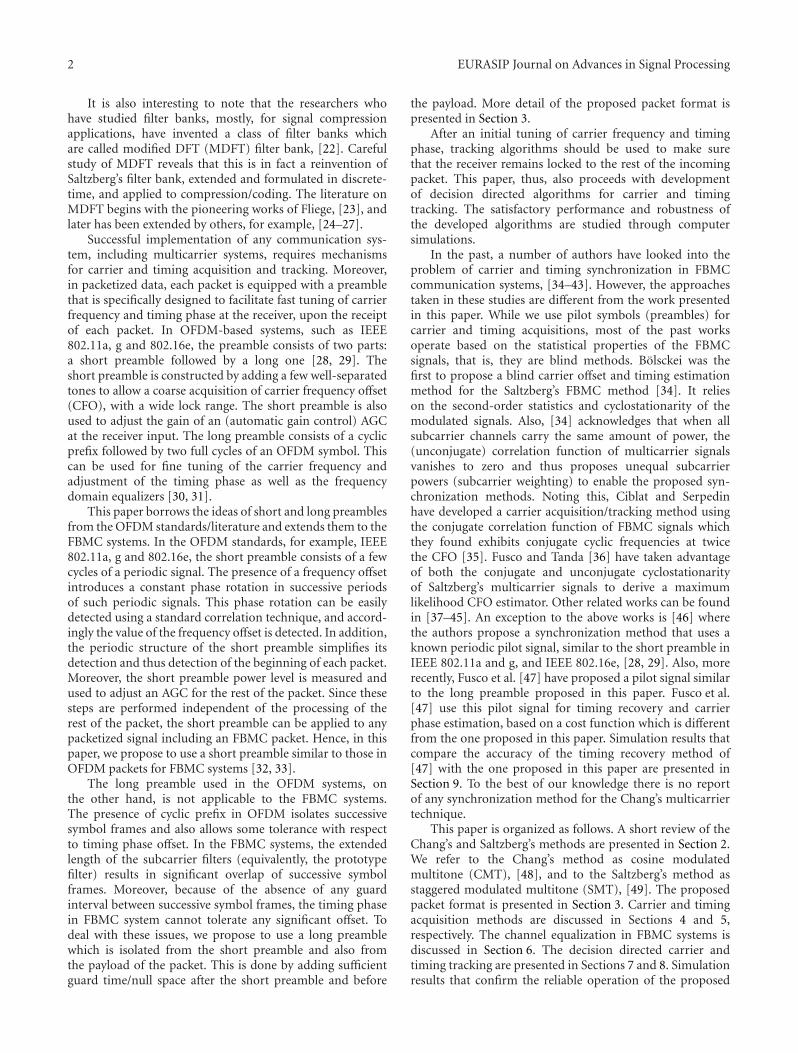
2 EURASIP Journal on Advances in Signal Processing
It is also interesting to note that the researchers whohave studied filter banks, mostly, for signal compressionapplications, have invented a class of filter banks whichare called modified DFT (MDFT) filter bank, [22]. Carefulstudy of MDFT reveals that this is in fact a reinvention ofSaltzberg’s filter bank, extended and formulated in discrete-time, and applied to compression/coding. The literature onMDFT begins with the pioneering works of Fliege, [23], andlater has been extended by others, for example, [24–27].
Successful implementation of any communication sys-tem, including multicarrier systems, requires mechanismsfor carrier and timing acquisition and tracking. Moreover,in packetized data, each packet is equipped with a preamblethat is specifically designed to facilitate fast tuning of carrierfrequency and timing phase at the receiver, upon the receiptof each packet. In OFDM-based systems, such as IEEE802.11a, g and 802.16e, the preamble consists of two parts:a short preamble followed by a long one [28, 29]. Theshort preamble is constructed by adding a few well-separatedtones to allow a coarse acquisition of carrier frequency offset(CFO), with a wide lock range. The short preamble is alsoused to adjust the gain of an (automatic gain control) AGCat the receiver input. The long preamble consists of a cyclicprefix followed by two full cycles of an OFDM symbol. Thiscan be used for fine tuning of the carrier frequency andadjustment of the timing phase as well as the frequencydomain equalizers [30, 31].
This paper borrows the ideas of short and long preamblesfrom the OFDM standards/literature and extends them to theFBMC systems. In the OFDM standards, for example, IEEE802.11a, g and 802.16e, the short preamble consists of a fewcycles of a periodic signal. The presence of a frequency offsetintroduces a constant phase rotation in successive periodsof such periodic signals. This phase rotation can be easilydetected using a standard correlation technique, and accord-ingly the value of the frequency offset is detected. In addition,the periodic structure of the short preamble simplifies itsdetection and thus detection of the beginning of each packet.Moreover, the short preamble power level is measured andused to adjust an AGC for the rest of the packet. Since thesesteps are performed independent of the processing of therest of the packet, the short preamble can be applied to anypacketized signal including an FBMC packet. Hence, in thispaper, we propose to use a short preamble similar to those inOFDM packets for FBMC systems [32, 33].
The long preamble used in the OFDM systems, onthe other hand, is not applicable to the FBMC systems.The presence of cyclic prefix in OFDM isolates successivesymbol frames and also allows some tolerance with respectto timing phase offset. In the FBMC systems, the extendedlength of the subcarrier filters (equivalently, the prototypefilter) results in significant overlap of successive symbolframes. Moreover, because of the absence of any guardinterval between successive symbol frames, the timing phasein FBMC system cannot tolerate any significant offset. Todeal with these issues, we propose to use a long preamblewhich is isolated from the short preamble and also fromthe payload of the packet. This is done by adding sufficientguard time/null space after the short preamble and before
the payload. More detail of the proposed packet format ispresented in Section 3.
After an initial tuning of carrier frequency and timingphase, tracking algorithms should be used to make surethat the receiver remains locked to the rest of the incomingpacket. This paper, thus, also proceeds with developmentof decision directed algorithms for carrier and timingtracking. The satisfactory performance and robustness ofthe developed algorithms are studied through computersimulations.
In the past, a number of authors have looked into theproblem of carrier and timing synchronization in FBMCcommunication systems, [34–43]. However, the approachestaken in these studies are different from the work presentedin this paper. While we use pilot symbols (preambles) forcarrier and timing acquisitions, most of the past worksoperate based on the statistical properties of the FBMCsignals, that is, they are blind methods. Bolsckei was thefirst to propose a blind carrier offset and timing estimationmethod for the Saltzberg’s FBMC method [34]. It relieson the second-order statistics and cyclostationarity of themodulated signals. Also, [34] acknowledges that when allsubcarrier channels carry the same amount of power, the(unconjugate) correlation function of multicarrier signalsvanishes to zero and thus proposes unequal subcarrierpowers (subcarrier weighting) to enable the proposed syn-chronization methods. Noting this, Ciblat and Serpedinhave developed a carrier acquisition/tracking method usingthe conjugate correlation function of FBMC signals whichthey found exhibits conjugate cyclic frequencies at twicethe CFO [35]. Fusco and Tanda [36] have taken advantageof both the conjugate and unconjugate cyclostationarityof Saltzberg’s multicarrier signals to derive a maximumlikelihood CFO estimator. Other related works can be foundin [37–45]. An exception to the above works is [46] wherethe authors propose a synchronization method that uses aknown periodic pilot signal, similar to the short preamble inIEEE 802.11a and g, and IEEE 802.16e, [28, 29]. Also, morerecently, Fusco et al. [47] have proposed a pilot signal similarto the long preamble proposed in this paper. Fusco et al.[47] use this pilot signal for timing recovery and carrierphase estimation, based on a cost function which is differentfrom the one proposed in this paper. Simulation results thatcompare the accuracy of the timing recovery method of[47] with the one proposed in this paper are presented inSection 9. To the best of our knowledge there is no reportof any synchronization method for the Chang’s multicarriertechnique.
This paper is organized as follows. A short review of theChang’s and Saltzberg’s methods are presented in Section 2.We refer to the Chang’s method as cosine modulatedmultitone (CMT), [48], and to the Saltzberg’s method asstaggered modulated multitone (SMT), [49]. The proposedpacket format is presented in Section 3. Carrier and timingacquisition methods are discussed in Sections 4 and 5,respectively. The channel equalization in FBMC systems isdiscussed in Section 6. The decision directed carrier andtiming tracking are presented in Sections 7 and 8. Simulationresults that confirm the reliable operation of the proposed
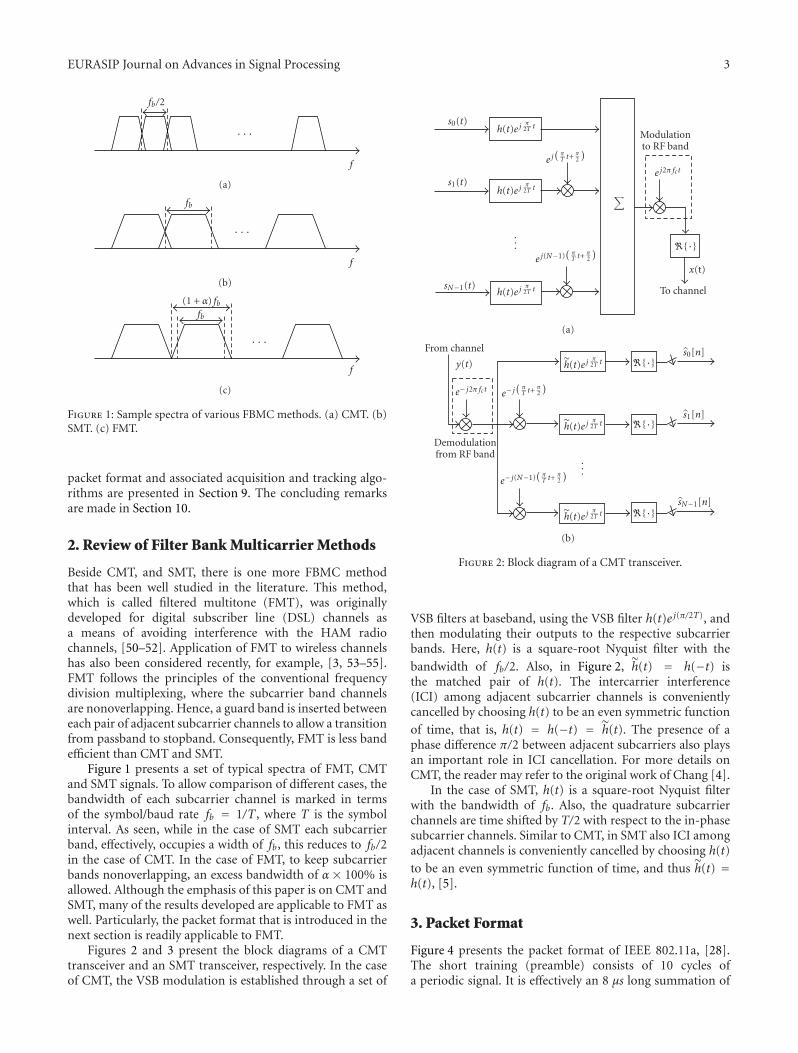
EURASIP Journal on Advances in Signal Processing 3
fb/2
· · ·
f
(a)
fb
· · ·
f
(b)
fb
· · ·
f
(1 + α) fb
(c)
Figure 1: Sample spectra of various FBMC methods. (a) CMT. (b)SMT. (c) FMT.
packet format and associated acquisition and tracking algo-rithms are presented in Section 9. The concluding remarksare made in Section 10.
2. Review of Filter Bank Multicarrier Methods
Beside CMT, and SMT, there is one more FBMC methodthat has been well studied in the literature. This method,which is called filtered multitone (FMT), was originallydeveloped for digital subscriber line (DSL) channels asa means of avoiding interference with the HAM radiochannels, [50–52]. Application of FMT to wireless channelshas also been considered recently, for example, [3, 53–55].FMT follows the principles of the conventional frequencydivision multiplexing, where the subcarrier band channelsare nonoverlapping. Hence, a guard band is inserted betweeneach pair of adjacent subcarrier channels to allow a transitionfrom passband to stopband. Consequently, FMT is less bandefficient than CMT and SMT.
Figure 1 presents a set of typical spectra of FMT, CMTand SMT signals. To allow comparison of different cases, thebandwidth of each subcarrier channel is marked in termsof the symbol/baud rate fb = 1/T , where T is the symbolinterval. As seen, while in the case of SMT each subcarrierband, effectively, occupies a width of fb, this reduces to fb/2in the case of CMT. In the case of FMT, to keep subcarrierbands nonoverlapping, an excess bandwidth of α × 100% isallowed. Although the emphasis of this paper is on CMT andSMT, many of the results developed are applicable to FMT aswell. Particularly, the packet format that is introduced in thenext section is readily applicable to FMT.
Figures 2 and 3 present the block diagrams of a CMTtransceiver and an SMT transceiver, respectively. In the caseof CMT, the VSB modulation is established through a set of
s0(t)h(t)e j
π2T t
s1(t)h(t)e j
π2T t
sN−1(t)h(t)e j
π2T t
...
e j(πT t+
π2
)
e j(N−1)(πT t+
π2
)
∑
Modulationto RF band
e j2π fct
�{·}
x(t)
To channel
(a)
From channel
y(t)
e− j2π fct
Demodulationfrom RF band
e− j(πT t+
π2
)
e− j(N−1)(πT t+
π2
)
h(t)e jπ
2T t
h(t)e jπ
2T t
h(t)e jπ
2T t
...
�{·}
�{·}
�{·}
s0[n]
s1[n]
sN−1[n]
(b)
Figure 2: Block diagram of a CMT transceiver.
VSB filters at baseband, using the VSB filter h(t)e j(π/2T), andthen modulating their outputs to the respective subcarrierbands. Here, h(t) is a square-root Nyquist filter with the
bandwidth of fb/2. Also, in Figure 2, h(t) = h(−t) isthe matched pair of h(t). The intercarrier interference(ICI) among adjacent subcarrier channels is convenientlycancelled by choosing h(t) to be an even symmetric function
of time, that is, h(t) = h(−t) = h(t). The presence of aphase difference π/2 between adjacent subcarriers also playsan important role in ICI cancellation. For more details onCMT, the reader may refer to the original work of Chang [4].
In the case of SMT, h(t) is a square-root Nyquist filterwith the bandwidth of fb. Also, the quadrature subcarrierchannels are time shifted by T/2 with respect to the in-phasesubcarrier channels. Similar to CMT, in SMT also ICI amongadjacent channels is conveniently cancelled by choosing h(t)
to be an even symmetric function of time, and thus h(t) =h(t), [5].
3. Packet Format
Figure 4 presents the packet format of IEEE 802.11a, [28].The short training (preamble) consists of 10 cycles ofa periodic signal. It is effectively an 8 μs long summation of
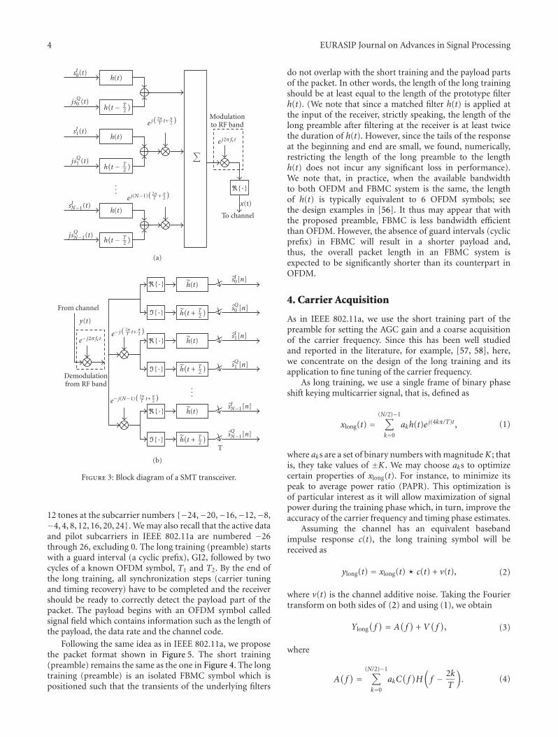
4 EURASIP Journal on Advances in Signal Processing
sI0(t)
jsQ0 (t)
sI1(t)
jsQ1 (t)
sIN−1(t)
jsQN−1(t)
h(t)
h(t − T
2
)
h(t)
h(t − T
2
)
h(t)
h(t − T
2
)
...
e j(
2πT t+ π
2
)
e j(N−1)(
2πT + π
2
)
∑
Modulationto RF band
e j2π fct
�{·}
x(t)
To channel
(a)
From channel
y(t)
e− j2π fct
Demodulationfrom RF band
e− j(
2πT t+ π
2
)
e− j(N−1)(
2πT t+ π
2
)
�{·}
�{·}
�{·}
�{·}
�{·}
�{·}
h(t)
h(t + T
2
)
h(t)
h(t + T
2
)
h(t)
h(t + T
2
)
...
sI0[n]
sQ0 [n]
sI1[n]
sQ1 [n]
sIN−1[n]
sQN−1[n]
T
(b)
Figure 3: Block diagram of a SMT transceiver.
12 tones at the subcarrier numbers {−24,−20,−16,−12,−8,−4, 4, 8, 12, 16, 20, 24}. We may also recall that the active dataand pilot subcarriers in IEEE 802.11a are numbered −26through 26, excluding 0. The long training (preamble) startswith a guard interval (a cyclic prefix), GI2, followed by twocycles of a known OFDM symbol, T1 and T2. By the end ofthe long training, all synchronization steps (carrier tuningand timing recovery) have to be completed and the receivershould be ready to correctly detect the payload part of thepacket. The payload begins with an OFDM symbol calledsignal field which contains information such as the length ofthe payload, the data rate and the channel code.
Following the same idea as in IEEE 802.11a, we proposethe packet format shown in Figure 5. The short training(preamble) remains the same as the one in Figure 4. The longtraining (preamble) is an isolated FBMC symbol which ispositioned such that the transients of the underlying filters
do not overlap with the short training and the payload partsof the packet. In other words, the length of the long trainingshould be at least equal to the length of the prototype filterh(t). (We note that since a matched filter h(t) is applied atthe input of the receiver, strictly speaking, the length of thelong preamble after filtering at the receiver is at least twicethe duration of h(t). However, since the tails of the responseat the beginning and end are small, we found, numerically,restricting the length of the long preamble to the lengthh(t) does not incur any significant loss in performance).We note that, in practice, when the available bandwidthto both OFDM and FBMC system is the same, the lengthof h(t) is typically equivalent to 6 OFDM symbols; seethe design examples in [56]. It thus may appear that withthe proposed preamble, FBMC is less bandwidth efficientthan OFDM. However, the absence of guard intervals (cyclicprefix) in FBMC will result in a shorter payload and,thus, the overall packet length in an FBMC system isexpected to be significantly shorter than its counterpart inOFDM.
4. Carrier Acquisition
As in IEEE 802.11a, we use the short training part of thepreamble for setting the AGC gain and a coarse acquisitionof the carrier frequency. Since this has been well studiedand reported in the literature, for example, [57, 58], here,we concentrate on the design of the long training and itsapplication to fine tuning of the carrier frequency.
As long training, we use a single frame of binary phaseshift keying multicarrier signal, that is, defined as
xlong(t) =(N/2)−1∑
k=0
akh(t)e j(4kπ/T)t, (1)
where aks are a set of binary numbers with magnitudeK ; thatis, they take values of ±K . We may choose aks to optimizecertain properties of xlong(t). For instance, to minimize itspeak to average power ratio (PAPR). This optimization isof particular interest as it will allow maximization of signalpower during the training phase which, in turn, improve theaccuracy of the carrier frequency and timing phase estimates.
Assuming the channel has an equivalent basebandimpulse response c(t), the long training symbol will bereceived as
ylong(t) = xlong(t)� c(t) + v(t), (2)
where v(t) is the channel additive noise. Taking the Fouriertransform on both sides of (2) and using (1), we obtain
Ylong(f) = A
(f)
+V(f), (3)
where
A(f) =
(N/2)−1∑
k=0
akC(f)H(f − 2k
T
). (4)
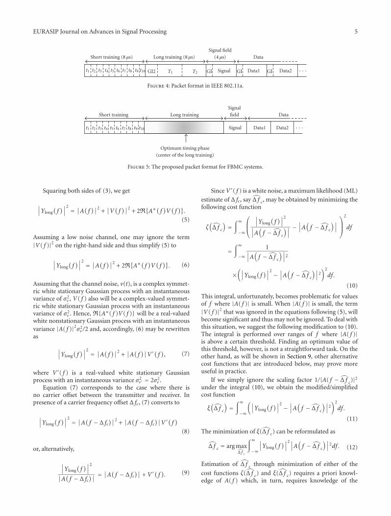
EURASIP Journal on Advances in Signal Processing 5
Short training (8 μs) Long training (8 μs)Signal field
(4 μs) Data
t1 t2 t3 t4 t5 t6 t7 t8 t9 t10 GI2 T1 T2 GI Signal GI Data1 GI Data2 · · ·
Figure 4: Packet format in IEEE 802.11a.
Short training Long trainingSignalfield Data
t1 t2 t3 t4 t5 t6 t7 t8 t9 t10 Signal Data1 Data2 · · ·
Optimum timing phase(center of the long training)
Figure 5: The proposed packet format for FBMC systems.
Squaring both sides of (3), we get
∣∣∣Ylong(f)∣∣∣
2 = ∣∣A( f )∣∣2 +∣∣V(f)∣∣2 + 2R
{A∗(f)V(f)}.
(5)
Assuming a low noise channel, one may ignore the term|V( f )|2 on the right-hand side and thus simplify (5) to
∣∣∣Ylong(f)∣∣∣
2 = ∣∣A( f )∣∣2 + 2R{A∗(f)V(f)}. (6)
Assuming that the channel noise, v(t), is a complex symmet-ric white stationary Gaussian process with an instantaneousvariance of σ2
v , V( f ) also will be a complex-valued symmet-ric white stationary Gaussian process with an instantaneousvariance of σ2
v . Hence, R{A∗( f )V( f )} will be a real-valuedwhite nonstationary Gaussian process with an instantaneousvariance |A( f )|2σ2
v /2 and, accordingly, (6) may be rewrittenas
∣∣∣Ylong(f)∣∣∣
2 = ∣∣A( f )∣∣2 +∣∣A(f)∣∣V ′( f
), (7)
where V ′( f ) is a real-valued white stationary Gaussianprocess with an instantaneous variance σ2
v′ = 2σ2v .
Equation (7) corresponds to the case where there isno carrier offset between the transmitter and receiver. Inpresence of a carrier frequency offset Δ fc, (7) converts to
∣∣∣Ylong(f)∣∣∣
2 = ∣∣A( f − Δ fc)∣∣2 +
∣∣A(f − Δ fc
)∣∣V ′( f)
(8)
or, alternatively,
∣∣∣Ylong(f)∣∣∣
2
∣∣A(f − Δ fc
)∣∣ =∣∣A(f − Δ fc
)∣∣ +V ′( f). (9)
SinceV ′( f ) is a white noise, a maximum likelihood (ML)
estimate of Δ fc, say Δ f c, may be obtained by minimizing thefollowing cost function
ζ(Δ f c
)=∫∞
−∞
⎛⎜⎝
∣∣∣Ylong(f)∣∣∣
2
∣∣∣A(f − Δ f c
)∣∣∣−∣∣∣A(f − Δ f c
)∣∣∣
⎞⎟⎠
2
df
=∫∞
−∞
1∣∣∣A(f − Δ f c
)∣∣∣2
×(∣∣∣Ylong
(f)∣∣∣
2 −∣∣∣A(f − Δ f c
)∣∣∣2)2
df .
(10)
This integral, unfortunately, becomes problematic for valuesof f where |A( f )| is small. When |A( f )| is small, the term|V( f )|2 that was ignored in the equations following (5), willbecome significant and thus may not be ignored. To deal withthis situation, we suggest the following modification to (10).The integral is performed over ranges of f where |A( f )|is above a certain threshold. Finding an optimum value ofthis threshold, however, is not a straightforward task. On theother hand, as will be shown in Section 9, other alternativecost functions that are introduced below, may prove moreuseful in practice.
If we simply ignore the scaling factor 1/|A( f − Δ f c)|2under the integral (10), we obtain the modified/simplifiedcost function
ξ(Δ f c
)=∫∞
−∞
(∣∣∣Ylong(f)∣∣∣
2 −∣∣∣A(f − Δ f c
)∣∣∣2)2
df .
(11)
The minimization of ξ(Δ f c) can be reformulated as
Δ f c = arg maxΔ f c
∫∞
−∞
∣∣∣Ylong(f)∣∣∣
2∣∣∣A(f − Δ f c
)∣∣∣2df . (12)
Estimation of Δ f c through minimization of either of the
cost functions ζ(Δ f c) and ξ(Δ f c) requires a priori knowl-edge of A( f ) which, in turn, requires knowledge of the
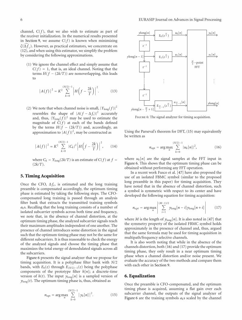
6 EURASIP Journal on Advances in Signal Processing
channel, C( f ), that we also wish to estimate as part ofthe receiver initialization. In the numerical results presentedin Section 9, we assume C( f ) is known when minimizing
ζ(Δ f c). However, as practical estimators, we concentrate on(12), and when using this estimator, we simplify the problemby considering the following approximations.
(1) We ignore the channel effect and simply assume thatC( f ) = 1, that is, an ideal channel. Noting that theterms H( f − (2k/T)) are nonoverlapping, this leadsto
∣∣A(f)∣∣2 = K2
(N/2)−1∑
k=0
∣∣∣∣H(f − 2k
T
)∣∣∣∣2
. (13)
(2) We note that when channel noise is small, |Ylong( f )|2resembles the shape of |A( f − Δ fc)|2 accuratelyand, thus, |Ylong( f )|2 may be used to estimate themagnitude of C( f ) at each of the bands definedby the terms H( f − (2k/T)) and, accordingly, anapproximation to |A( f )|2, may be constructed as
∣∣A(f)∣∣2 = K2
(N/2)−1∑
k=0
|Ck|2∣∣∣∣H(f − 2k
T
)∣∣∣∣2
, (14)
where Ck = Ylong(2k/T) is an estimate of C( f ) at f =(2k/T).
5. Timing Acquisition
Once the CFO, Δ fc, is estimated and the long trainingpreamble is compensated accordingly, the optimum timingphase is estimated by taking the following steps. The CFO-compensated long training is passed through an analysisfilter bank that extracts the transmitted training symbolsaks. Recalling that the long training consists of a number ofisolated subcarrier symbols across both time and frequency,we note that, in the absence of channel distortion, at theoptimum timing phase, the analyzed subcarrier signals reachtheir maximum amplitudes independent of one another. Thepresence of channel introduces some distortion in the signalsuch that the optimum timing phase may not be the same fordifferent subcarriers. It is thus reasonable to check the energyof the analyzed signals and choose the timing phase thatmaximizes the total energy of demodulated signals across allthe subcarriers.
Figure 6 presents the signal analyzer that we propose fortiming acquisition. It is a polyphase filter bank with N/2bands, with E0(z) through E(N/2)−1(z) being the polyphasecomponents of the prototype filter h[n]; a discrete-timeversion of h(t). The input ylong[n] is a sampled version ofylong(t). The optimum timing phase is, thus, obtained as
nopt = arg maxn
(N/2)−1∑
k=0
∣∣yk[n]∣∣2. (15)
ylong[n]
z−1
ylong[n− 1]
z−1
z−1
ylong[n− N
2 + 1]
E0(zN2)
E1(zN2)
E N2 −1
(zN2)
u0[n]
u1[n]
u N2 −1[n]
...
N2 −point
FFT
y0[n]
y1[n]
ylong[n]
...
Figure 6: The signal analyzer for timing acquisition.
Using the Parseval’s theorem for DFT, (15) may equivalentlybe written as
nopt = arg maxn
(N/2)−1∑
k=0
|uk[n]|2, (16)
where uk[n] are the signal samples at the FFT input inFigure 6. This shows that the optimum timing phase can beobtained without performing any FFT operation.
In a recent work Fusco et al. [47] have also proposed theuse of an isolated FBMC symbol (similar to the proposedlong preamble in this paper) for timing acquisition. Theyhave noted that in the absence of channel distortion, sucha symbol is symmetric with respect to its center and havedeveloped the following equation for timing acquisition:
nopt = arg maxn
∣∣∣∣∣∣
(M−1)/2∑
i=1
ylong[n− i]ylong[n + i]
∣∣∣∣∣∣(17)
where M is the length of ylong[n]. It is also noted in [47] thatthe symmetry property of the isolated FBMC symbol holdsapproximately in the presence of channel and, thus, arguedthat the same formula may be used for timing acquisition inmultipath/frequency selective channels.
It is also worth noting that while in the absence of thechannels distortion, both (16) and (17) provide the optimumtiming phase, they only result in a near optimum timingphase when a channel distortion and/or noise present. Weevaluate the accuracy of the two methods and compare themwith each other in Section 9.
6. Equalization
Once the preamble is CFO-compensated, and the optimumtiming phase is acquired, assuming a flat gain over eachsubcarrier channel, the outputs of the signal analyzer ofFigure 6 are the training symbols aks scaled by the channel
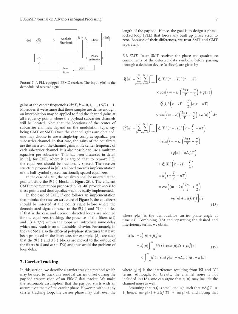
EURASIP Journal on Advances in Signal Processing 7
y[n]
e− j
Analysisfilter bank
Loopfilter
sk[n]s
ϕ[n]
Slicer
Phaseestimator
sk[n]s
Figure 7: A PLL equipped FBMC receiver. The input y[n] is thedemodulated received signal.
gains at the center frequencies 2k/T , k = 0, 1, . . . , (N/2) − 1.Moreover, if we assume that these samples are dense enough,an interpolation may be applied to find the channel gains atall frequency points where the payload subcarrier channelswill be located. Note that the locations of the center ofsubcarrier channels depend on the modulation type, say,being CMT or SMT. Once the channel gains are obtained,one may choose to use a single-tap complex equalizer persubcarrier channel. In that case, the gains of the equalizersare the inverse of the channel gains at the center frequency ofeach subcarrier channel. It is also possible to use a multitapequalizer per subcarrier. This has been discussed in detailin [8], for SMT, where it is argued that to remove ICI,the equalizers should be fractionally spaced. The receiverstructure proposed in [8] is tailored towards implementationof the half-symbol spaced fractionally spaced equalizers.
In the case of CMT, the equalizers shall be inserted at thepoints before the R{·} blocks in Figure 2(b). The efficientCMT implementations proposed in [21, 48] provide access tothese points and thus equalizers can be easily implemented.
In the case of SMT, if one follows an implementationthat mimics the receiver structure of Figure 3, the equalizersshould be inserted at the points right before where thedemodulated signals branch to the R{·} and I{·} blocks.If that is the case and decision directed loops are adoptedfor the equalizers tracking, the presence of the filters h(t)and h(t + T/2) within the loops will introduce some delaywhich may result in an undesirable behavior. Fortunately, inthe case SMT also the efficient polyphase structures that havebeen proposed in the literature, for example, [8], are suchthat the R{·} and I{·} blocks are moved to the output ofthe filters h(t) and h(t + T/2) and thus avoid the problem ofloop delay.
7. Carrier Tracking
In this section, we describe a carrier tracking method whichmay be used to track any residual carrier offset during thepayload transmission of an FBMC data packet. We makethe reasonable assumption that the payload starts with anaccurate estimate of the carrier phase. However, without anycarrier tracking loop, the carrier phase may drift over the
length of the payload. Hence, the goal is to design a phase-locked loop (PLL) that forces any built up phase error tozero. Because of their differences, we treat SMT and CMTseparately.
7.1. SMT. In an SMT receiver, the phase and quadraturecomponents of the detected data symbols, before passingthrough a decision device (a slicer), are given by
sIk[n] =∞∑
l=−∞
N−1∑
m=0
∫∞
−∞
[sIm[l]h(τ − lT)h(τ − nT)
× cos(
(m− k)(
2πτT
+π
2
)+ ϕ[n]
)
− sQm[l]h(τ − lT − T
2
)h(τ − nT)
× sin(
(m− k)(
2πτT
+π
2
)+ϕ[n]
)]dτ
sQk [n] =∞∑
l=−∞
N−1∑
m=0
∫∞
−∞
[sIm[l]h(τ − lT)h
(τ +
T
2− nT
)
× sin(
(m− k)(
2πτT
+π
2
)
+ϕ[n] + πΔ fcT)
+ sQm[l]h(τ − lT +
T
2
)
× h(τ+
T
2− nT
)
× cos(
(m− k)(
2πτT
+π
2
)
+ϕ[n] + πΔ fcT)]dτ,
(18)
where ϕ[n] is the demodulator carrier phase angle attime nT . Combining (18) and separating the desired andinterference terms, we obtain
sk[n] = sIk[n] + jsQk [n]
= sIk[n]∫∞
−∞h2(τ) cosϕ[n]dτ + jsQk [n]
×∫∞
−∞h2(τ) sin
(ϕ[n] + πΔ fcT
)dτ + ιk[n]
(19)
where ιk[n] is the interference resulting from ISI and ICIterms. Although, for brevity, the channel noise is notincluded in (18), one can argue that ιk[n] may include thechannel noise as well.
Assuming that Δ fc is small enough such that πΔ fcT �1, hence, sin(ϕ[n] + πΔ fcT) ≈ sinϕ[n], and noting that
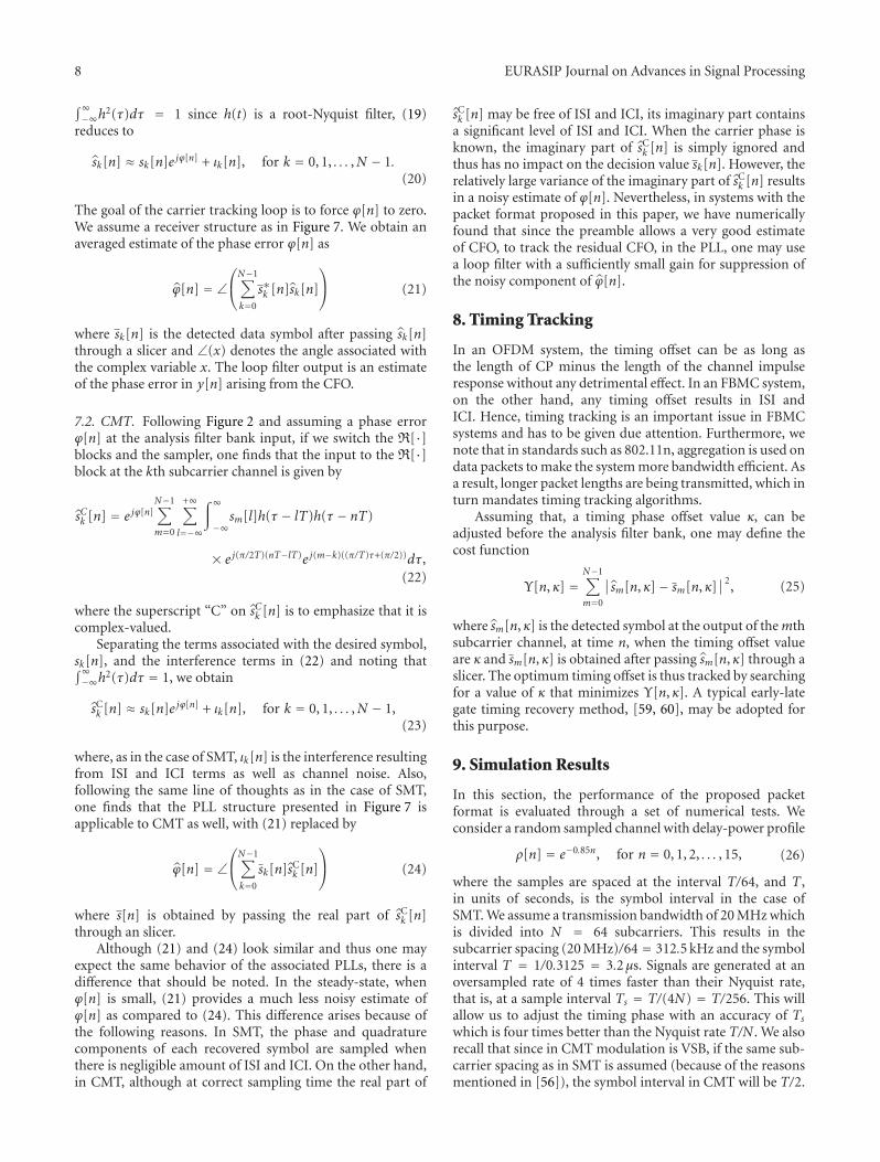
8 EURASIP Journal on Advances in Signal Processing
∫∞−∞h
2(τ)dτ = 1 since h(t) is a root-Nyquist filter, (19)reduces to
sk[n] ≈ sk[n]e jϕ[n] + ιk[n], for k = 0, 1, . . . ,N − 1.(20)
The goal of the carrier tracking loop is to force ϕ[n] to zero.We assume a receiver structure as in Figure 7. We obtain anaveraged estimate of the phase error ϕ[n] as
ϕ[n] = ∠⎛⎝N−1∑
k=0
s∗k [n]sk[n]
⎞⎠ (21)
where sk[n] is the detected data symbol after passing sk[n]through a slicer and ∠(x) denotes the angle associated withthe complex variable x. The loop filter output is an estimateof the phase error in y[n] arising from the CFO.
7.2. CMT. Following Figure 2 and assuming a phase errorϕ[n] at the analysis filter bank input, if we switch the R[·]blocks and the sampler, one finds that the input to the R[·]block at the kth subcarrier channel is given by
sCk [n] = e jϕ[n]N−1∑
m=0
+∞∑
l=−∞
∫∞
−∞sm[l]h(τ − lT)h(τ − nT)
× e j(π/2T)(nT−lT)e j(m−k)((π/T)τ+(π/2))dτ,(22)
where the superscript “C” on sCk [n] is to emphasize that it iscomplex-valued.
Separating the terms associated with the desired symbol,sk[n], and the interference terms in (22) and noting that∫∞−∞h
2(τ)dτ = 1, we obtain
sCk [n] ≈ sk[n]e jϕ[n] + ιk[n], for k = 0, 1, . . . ,N − 1,(23)
where, as in the case of SMT, ιk[n] is the interference resultingfrom ISI and ICI terms as well as channel noise. Also,following the same line of thoughts as in the case of SMT,one finds that the PLL structure presented in Figure 7 isapplicable to CMT as well, with (21) replaced by
ϕ[n] = ∠⎛⎝N−1∑
k=0
sk[n]sCk [n]
⎞⎠ (24)
where s[n] is obtained by passing the real part of sCk [n]through an slicer.
Although (21) and (24) look similar and thus one mayexpect the same behavior of the associated PLLs, there is adifference that should be noted. In the steady-state, whenϕ[n] is small, (21) provides a much less noisy estimate ofϕ[n] as compared to (24). This difference arises because ofthe following reasons. In SMT, the phase and quadraturecomponents of each recovered symbol are sampled whenthere is negligible amount of ISI and ICI. On the other hand,in CMT, although at correct sampling time the real part of
sCk [n] may be free of ISI and ICI, its imaginary part containsa significant level of ISI and ICI. When the carrier phase isknown, the imaginary part of sCk [n] is simply ignored andthus has no impact on the decision value sk[n]. However, therelatively large variance of the imaginary part of sCk [n] resultsin a noisy estimate of ϕ[n]. Nevertheless, in systems with thepacket format proposed in this paper, we have numericallyfound that since the preamble allows a very good estimateof CFO, to track the residual CFO, in the PLL, one may usea loop filter with a sufficiently small gain for suppression ofthe noisy component of ϕ[n].
8. Timing Tracking
In an OFDM system, the timing offset can be as long asthe length of CP minus the length of the channel impulseresponse without any detrimental effect. In an FBMC system,on the other hand, any timing offset results in ISI andICI. Hence, timing tracking is an important issue in FBMCsystems and has to be given due attention. Furthermore, wenote that in standards such as 802.11n, aggregation is used ondata packets to make the system more bandwidth efficient. Asa result, longer packet lengths are being transmitted, which inturn mandates timing tracking algorithms.
Assuming that, a timing phase offset value κ, can beadjusted before the analysis filter bank, one may define thecost function
Υ[n, κ] =N−1∑
m=0
∣∣sm[n, κ]− sm[n, κ]∣∣2, (25)
where sm[n, κ] is the detected symbol at the output of themthsubcarrier channel, at time n, when the timing offset valueare κ and sm[n, κ] is obtained after passing sm[n, κ] through aslicer. The optimum timing offset is thus tracked by searchingfor a value of κ that minimizes Υ[n, κ]. A typical early-lategate timing recovery method, [59, 60], may be adopted forthis purpose.
9. Simulation Results
In this section, the performance of the proposed packetformat is evaluated through a set of numerical tests. Weconsider a random sampled channel with delay-power profile
ρ[n] = e−0.85n, for n = 0, 1, 2, . . . , 15, (26)
where the samples are spaced at the interval T/64, and T ,in units of seconds, is the symbol interval in the case ofSMT. We assume a transmission bandwidth of 20 MHz whichis divided into N = 64 subcarriers. This results in thesubcarrier spacing (20 MHz)/64 = 312.5 kHz and the symbolinterval T = 1/0.3125 = 3.2μs. Signals are generated at anoversampled rate of 4 times faster than their Nyquist rate,that is, at a sample interval Ts = T/(4N) = T/256. This willallow us to adjust the timing phase with an accuracy of Tswhich is four times better than the Nyquist rate T/N . We alsorecall that since in CMT modulation is VSB, if the same sub-carrier spacing as in SMT is assumed (because of the reasonsmentioned in [56]), the symbol interval in CMT will be T/2.
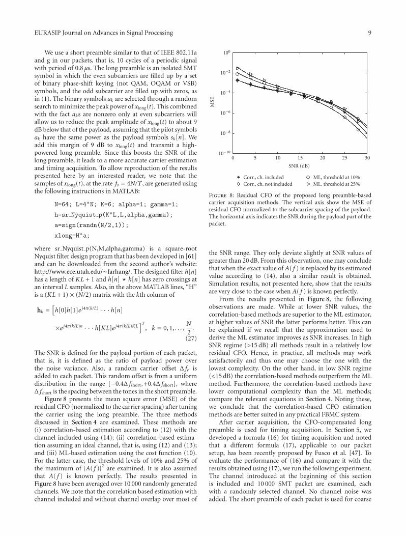
EURASIP Journal on Advances in Signal Processing 9
We use a short preamble similar to that of IEEE 802.11aand g in our packets, that is, 10 cycles of a periodic signalwith period of 0.8 μs. The long preamble is an isolated SMTsymbol in which the even subcarriers are filled up by a setof binary phase-shift keying (not QAM, OQAM or VSB)symbols, and the odd subcarrier are filled up with zeros, asin (1). The binary symbols ak are selected through a randomsearch to minimize the peak power of xlong(t). This combinedwith the fact aks are nonzero only at even subcarriers willallow us to reduce the peak amplitude of xlong(t) to about 9dB below that of the payload, assuming that the pilot symbolsak have the same power as the payload symbols sk[n]. Weadd this margin of 9 dB to xlong(t) and transmit a high-powered long preamble. Since this boosts the SNR of thelong preamble, it leads to a more accurate carrier estimationand timing acquisition. To allow reproduction of the resultspresented here by an interested reader, we note that thesamples of xlong(t), at the rate fs = 4N/T , are generated usingthe following instructions in MATLAB:
N=64; L=4∗N; K=6; alpha=1; gamma=1;
h=sr Nyquist p(K∗L,L,alpha,gamma);
a=sign(randn(N/2,1));
xlong=H∗a;
where sr Nyquist p(N,M,alpha,gamma) is a square-rootNyquist filter design program that has been developed in [61]and can be downloaded from the second author’s website:http://www.ece.utah.edu/∼farhang/. The designed filter h[n]has a length of KL + 1 and h[n]� h[n] has zero crossings atan interval L samples. Also, in the above MATLAB lines, “H”is a (KL + 1)× (N/2) matrix with the kth column of
hk =[h[0]h[1]e j4π(k/L) · · ·h[n]
×e j4π(k/L)n · · ·h[KL]e j4π(k/L)KL]T
, k = 0, 1, . . . ,N
2.
(27)
The SNR is defined for the payload portion of each packet,that is, it is defined as the ratio of payload power overthe noise variance. Also, a random carrier offset Δ fc isadded to each packet. This random offset is from a uniformdistribution in the range [−0.4Δ fshort, +0.4Δ fshort], whereΔ fshort is the spacing between the tones in the short preamble.
Figure 8 presents the mean square error (MSE) of theresidual CFO (normalized to the carrier spacing) after tuningthe carrier using the long preamble. The three methodsdiscussed in Section 4 are examined. These methods are(i) correlation-based estimation according to (12) with thechannel included using (14); (ii) correlation-based estima-tion assuming an ideal channel, that is, using (12) and (13);and (iii) ML-based estimation using the cost function (10).For the latter case, the threshold levels of 10% and 25% ofthe maximum of |A( f )|2 are examined. It is also assumedthat A( f ) is known perfectly. The results presented inFigure 8 have been averaged over 10 000 randomly generatedchannels. We note that the correlation based estimation withchannel included and without channel overlap over most of
MSE
10−10
10−8
10−6
10−4
10−2
100
SNR (dB)
0 5 10 15 20 25 30
Corr., ch. includedCorr., ch. not included
ML, threshold at 10%ML, threshold at 25%
Figure 8: Residual CFO of the proposed long preamble-basedcarrier acquisition methods. The vertical axis show the MSE ofresidual CFO normalized to the subcarrier spacing of the payload.The horizontal axis indicates the SNR during the payload part of thepacket.
the SNR range. They only deviate slightly at SNR values ofgreater than 20 dB. From this observation, one may concludethat when the exact value of A( f ) is replaced by its estimatedvalue according to (14), also a similar result is obtained.Simulation results, not presented here, show that the resultsare very close to the case when A( f ) is known perfectly.
From the results presented in Figure 8, the followingobservations are made. While at lower SNR values, thecorrelation-based methods are superior to the ML estimator,at higher values of SNR the latter performs better. This canbe explained if we recall that the approximation used toderive the ML estimator improves as SNR increases. In highSNR regime (>15 dB) all methods result in a relatively lowresidual CFO. Hence, in practice, all methods may worksatisfactorily and thus one may choose the one with thelowest complexity. On the other hand, in low SNR regime(<15 dB) the correlation-based methods outperform the MLmethod. Furthermore, the correlation-based methods havelower computational complexity than the ML methods;compare the relevant equations in Section 4. Noting these,we conclude that the correlation-based CFO estimationmethods are better suited in any practical FBMC system.
After carrier acquisition, the CFO-compensated longpreamble is used for timing acquisition. In Section 5, wedeveloped a formula (16) for timing acquisition and notedthat a different formula (17), applicable to our packetsetup, has been recently proposed by Fusco et al. [47]. Toevaluate the performance of (16) and compare it with theresults obtained using (17), we run the following experiment.The channel introduced at the beginning of this sectionis included and 10 000 SMT packet are examined, eachwith a randomly selected channel. No channel noise wasadded. The short preamble of each packet is used for coarse
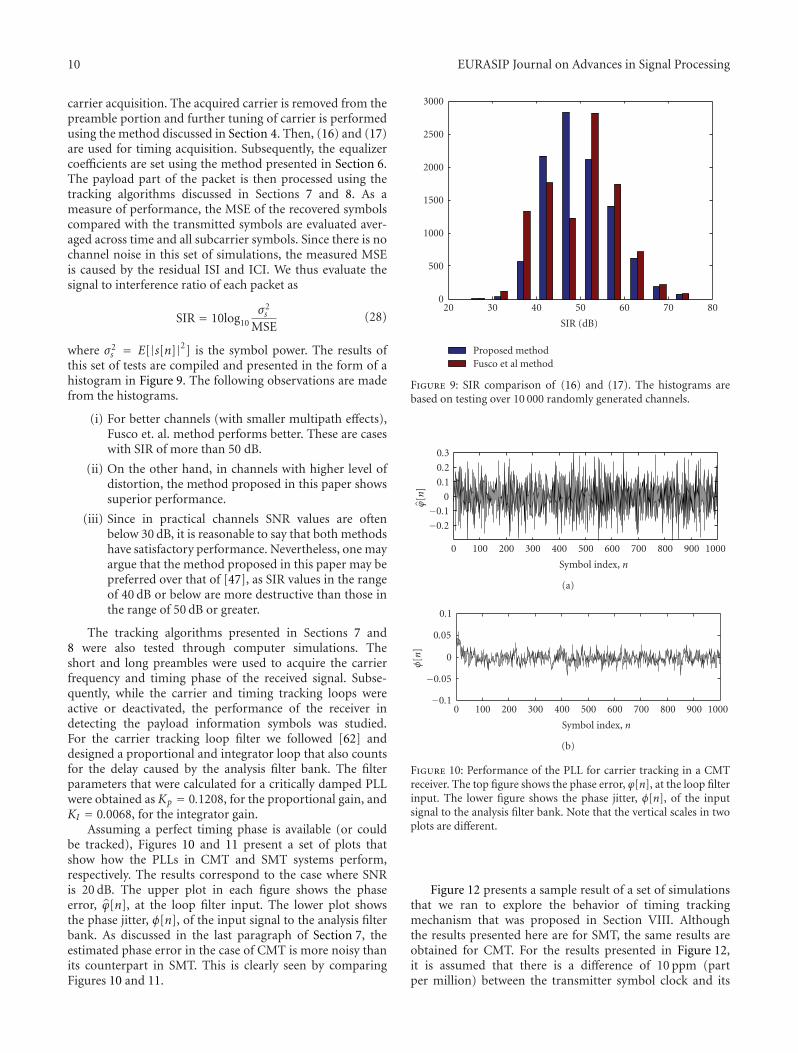
10 EURASIP Journal on Advances in Signal Processing
carrier acquisition. The acquired carrier is removed from thepreamble portion and further tuning of carrier is performedusing the method discussed in Section 4. Then, (16) and (17)are used for timing acquisition. Subsequently, the equalizercoefficients are set using the method presented in Section 6.The payload part of the packet is then processed using thetracking algorithms discussed in Sections 7 and 8. As ameasure of performance, the MSE of the recovered symbolscompared with the transmitted symbols are evaluated aver-aged across time and all subcarrier symbols. Since there is nochannel noise in this set of simulations, the measured MSEis caused by the residual ISI and ICI. We thus evaluate thesignal to interference ratio of each packet as
SIR = 10log10σ2s
MSE(28)
where σ2s = E[|s[n]|2] is the symbol power. The results of
this set of tests are compiled and presented in the form of ahistogram in Figure 9. The following observations are madefrom the histograms.
(i) For better channels (with smaller multipath effects),Fusco et. al. method performs better. These are caseswith SIR of more than 50 dB.
(ii) On the other hand, in channels with higher level ofdistortion, the method proposed in this paper showssuperior performance.
(iii) Since in practical channels SNR values are oftenbelow 30 dB, it is reasonable to say that both methodshave satisfactory performance. Nevertheless, one mayargue that the method proposed in this paper may bepreferred over that of [47], as SIR values in the rangeof 40 dB or below are more destructive than those inthe range of 50 dB or greater.
The tracking algorithms presented in Sections 7 and8 were also tested through computer simulations. Theshort and long preambles were used to acquire the carrierfrequency and timing phase of the received signal. Subse-quently, while the carrier and timing tracking loops wereactive or deactivated, the performance of the receiver indetecting the payload information symbols was studied.For the carrier tracking loop filter we followed [62] anddesigned a proportional and integrator loop that also countsfor the delay caused by the analysis filter bank. The filterparameters that were calculated for a critically damped PLLwere obtained as Kp = 0.1208, for the proportional gain, andKI = 0.0068, for the integrator gain.
Assuming a perfect timing phase is available (or couldbe tracked), Figures 10 and 11 present a set of plots thatshow how the PLLs in CMT and SMT systems perform,respectively. The results correspond to the case where SNRis 20 dB. The upper plot in each figure shows the phaseerror, ϕ[n], at the loop filter input. The lower plot showsthe phase jitter, φ[n], of the input signal to the analysis filterbank. As discussed in the last paragraph of Section 7, theestimated phase error in the case of CMT is more noisy thanits counterpart in SMT. This is clearly seen by comparingFigures 10 and 11.
0
500
1000
1500
2000
2500
3000
SIR (dB)
20 30 40 50 60 70 80
Proposed methodFusco et al method
Figure 9: SIR comparison of (16) and (17). The histograms arebased on testing over 10 000 randomly generated channels.
ϕ[n
]
−0.2
−0.1
0
0.1
0.2
0.3
Symbol index, n
0 100 200 300 400 500 600 700 800 900 1000
(a)
φ[n
]
−0.1
−0.05
0
0.05
0.1
Symbol index, n
0 100 200 300 400 500 600 700 800 900 1000
(b)
Figure 10: Performance of the PLL for carrier tracking in a CMTreceiver. The top figure shows the phase error, ϕ[n], at the loop filterinput. The lower figure shows the phase jitter, φ[n], of the inputsignal to the analysis filter bank. Note that the vertical scales in twoplots are different.
Figure 12 presents a sample result of a set of simulationsthat we ran to explore the behavior of timing trackingmechanism that was proposed in Section VIII. Althoughthe results presented here are for SMT, the same results areobtained for CMT. For the results presented in Figure 12,it is assumed that there is a difference of 10 ppm (partper million) between the transmitter symbol clock and its
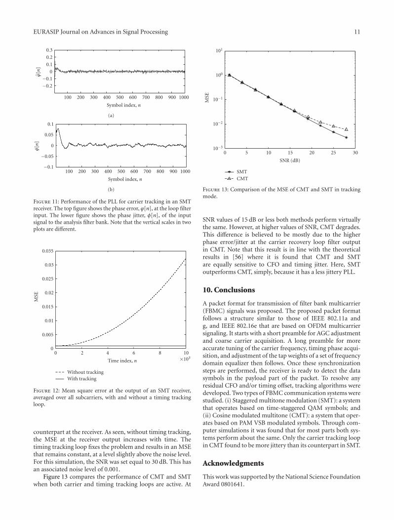
EURASIP Journal on Advances in Signal Processing 11ϕ
[n]
−0.2
−0.1
0
0.1
0.2
0.3
Symbol index, n
100 200 300 400 500 600 700 800 900 1000
(a)
φ[n
]
−0.1
−0.05
0
0.05
0.1
Symbol index, n
100 200 300 400 500 600 700 800 900 1000
(b)
Figure 11: Performance of the PLL for carrier tracking in an SMTreceiver. The top figure shows the phase error, ϕ[n], at the loop filterinput. The lower figure shows the phase jitter, φ[n], of the inputsignal to the analysis filter bank. Note that the vertical scales in twoplots are different.
MSE
0
0.005
0.01
0.015
0.02
0.025
0.03
0.035
Time index, n
0 2 4 6 8 10×103
Without trackingWith tracking
Figure 12: Mean square error at the output of an SMT receiver,averaged over all subcarriers, with and without a timing trackingloop.
counterpart at the receiver. As seen, without timing tracking,the MSE at the receiver output increases with time. Thetiming tracking loop fixes the problem and results in an MSEthat remains constant, at a level slightly above the noise level.For this simulation, the SNR was set equal to 30 dB. This hasan associated noise level of 0.001.
Figure 13 compares the performance of CMT and SMTwhen both carrier and timing tracking loops are active. At
MSE
10−3
10−2
10−1
100
101
SNR (dB)
0 5 10 15 20 25 30
SMTCMT
Figure 13: Comparison of the MSE of CMT and SMT in trackingmode.
SNR values of 15 dB or less both methods perform virtuallythe same. However, at higher values of SNR, CMT degrades.This difference is believed to be mostly due to the higherphase error/jitter at the carrier recovery loop filter outputin CMT. Note that this result is in line with the theoreticalresults in [56] where it is found that CMT and SMTare equally sensitive to CFO and timing jitter. Here, SMToutperforms CMT, simply, because it has a less jittery PLL.
10. Conclusions
A packet format for transmission of filter bank multicarrier(FBMC) signals was proposed. The proposed packet formatfollows a structure similar to those of IEEE 802.11a andg, and IEEE 802.16e that are based on OFDM multicarriersignaling. It starts with a short preamble for AGC adjustmentand coarse carrier acquisition. A long preamble for moreaccurate tuning of the carrier frequency, timing phase acqui-sition, and adjustment of the tap weights of a set of frequencydomain equalizer then follows. Once these synchronizationsteps are performed, the receiver is ready to detect the datasymbols in the payload part of the packet. To resolve anyresidual CFO and/or timing offset, tracking algorithms weredeveloped. Two types of FBMC communication systems werestudied. (i) Staggered multitone modulation (SMT): a systemthat operates based on time-staggered QAM symbols; and(ii) Cosine modulated multitone (CMT): a system that oper-ates based on PAM VSB modulated symbols. Through com-puter simulations it was found that for most parts both sys-tems perform about the same. Only the carrier tracking loopin CMT found to be more jittery than its counterpart in SMT.
Acknowledgments
This work was supported by the National Science FoundationAward 0801641.
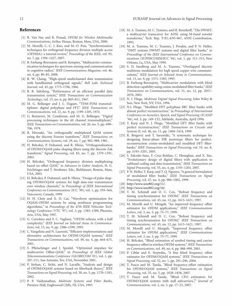
12 EURASIP Journal on Advances in Signal Processing
References
[1] R. Van Nee and R. Prasad, OFDM for Wireless MultimediaCommunications, Arthec House, Boston, Mass, USA, 2000.
[2] M. Morelli, C.-C. J. Kuo, and M.-O. Pun, “Synchronizationtechniques for orthogonal frequency division multiple access(OFDMA): a tutorial review,” Proceedings of the IEEE, vol. 95,no. 7, pp. 1394–1427, 2007.
[3] B. Farhang-Boroujeny and R. Kempter, “Multicarrier commu-nication techniques for spectrum sensing and communicationin cognitive radios,” IEEE Communications Magazine, vol. 46,no. 4, pp. 80–85, 2008.
[4] R. W. Chang, “High-speed multichannel data transmissionwith bandlimited orthogonal signals,” Bell Labs TechnicalJournal, vol. 45, pp. 1775–1796, 1966.
[5] B. R. Saltzberg, “Performance of an efficient parallel datatransmission system,” IEEE Transactions on CommunicationTechnology, vol. 15, no. 6, pp. 805–811, 1967.
[6] M. G. Bellanger and J. L. Daguet, “TDM-FDM transmul-tiplexer: digital polyphase and FFT,” IEEE Transactions onCommunications, vol. 22, no. 9, pp. 1199–1205, 1974.
[7] G. Bonnerot, M. Coudreuse, and M. G. Bellanger, “Digitalprocessing techniques in the 60 channel transmultiplexer,”IEEE Transactions on Communications, vol. 26, no. 5, pp. 698–706, 1978.
[8] B. Hirosaki, “An orthogonally multiplexed QAM systemusing the discrete Fourier transform,” IEEE Transactions onCommunications Systems, vol. 29, no. 7, pp. 982–989, 1981.
[9] H. Bolcskei, P. Duhamel, and R. Hleiss, “Orthogonalizationof OFDM/OQAM pulse shaping filters using the discrete Zaktransform,” Signal Processing, vol. 83, no. 7, pp. 1379–1391,2003.
[10] H. Bolcskei, “Orthogonal frequency division multiplexingbased on offset QAM,” in Advances in Gabor Analysis, H. G.Feichtinger and T. Strohmer, Eds., Birkhauser, Boston, Mass,USA, 2003.
[11] H. Bolcskei, P. Duhamel, and R. Hleiss, “Design of pulse shap-ing OFDM/OQAM systems for high data-rate transmissionover wireless channels,” in Proceedings of IEEE InternationalConference on Communications (ICC ’99), vol. 1, pp. 559–564,Vancouver, Canada, 1999.
[12] H. H. Chen and X. D. Cai, “Waveform optimization forOQAM-OFDM systems by using nonlinear programmingalgorithms,” in Proceedings of the 47th IEEE Vehicular Tech-nology Conference (VTC ’97), vol. 3, pp. 1385–1389, Phoenix,Ariz, USA, May 1997.
[13] G. Cariolaro and F. C. Vagliani, “OFDM scheme with a halfcomplexity,” IEEE Journal on Selected Areas in Communica-tions, vol. 13, no. 9, pp. 1586–1599, 1995.
[14] L. Vangelista and N. Laurenti, “Efficient implementations andalternative architectures for OFDM-OQAM systems,” IEEETransactions on Communications, vol. 49, no. 4, pp. 664–675,2001.
[15] S. Pfletschinger and J. Speidel, “Optimized impulses formulticarrier Offset-QAM,” in Proceedings of IEEE GlobalTelecommunications Conference (GLOBECOM ’01), vol. 1, pp.207–211, San Antonio, Tex, USA, November 2001.
[16] P. Siohan, C. Siclet, and N. Lacaille, “Analysis and designof OFDM/OQAM systems based on filterbank theory,” IEEETransactions on Signal Processing, vol. 50, no. 5, pp. 1170–1183,2002.
[17] P. P. Vaidyanathan, Multirate Systems and Filter Banks,Prentice-Hall, Englewood Cliffs, NJ, USA, 1993.
[18] M. A. Tzannes, M. C. Tzannes, and H. Resnikoff, “The DWMT:a multicarrier transceiver for ADSL using M-band wavelettransforms,” Tech. Rep. T1E1.4/93-067, ANSI Contribution,1993.
[19] M. A. Tzannes, M. C. Tzannes, J. Proakis, and P. N. Heller,“DMT systems DWMT systems and digital filter banks,” inProceedings of the IEEE International Conference on Commu-nications (SUPERCOMM/ICC ’94), vol. 1, pp. 311–315, NewOrleans, La, USA, May 1994.
[20] S. D. Sandberg and M. A. Tzannes, “Overlapped discretemultitone modulation for high speed copper wire communi-cations,” IEEE Journal on Selected Areas in Communications,vol. 13, no. 9, pp. 1571–1585, 1995.
[21] B. Farhang-Boroujeny, “Multicarrier modulation with blinddetection capability using cosine modulated filter banks,” IEEETransactions on Communications, vol. 51, no. 12, pp. 2057–2070, 2003.
[22] N. J. Fliege, Multirate Digital Signal Processing, John Wiley &Son, New York, NY, USA, 1994.
[23] N.J. Fliege, “Modified DFT polyphase SBC filter banks withalmost perfect reconstruction,” in Proceedings of InternationalConference on Acoustics, Speech, and Signal Processing (ICASSP’94), vol. 3, pp. 149–152, Adelaide, Australia, April 1994.
[24] T. Karp and N. J. Fliege, “Modified DFT filter banks withperfect reconstruction,” IEEE Transactions on Circuits andSystems II, vol. 46, no. 11, pp. 1404–1414, 1999.
[25] R. Bregovic and T. Saramaki, “A systematic technique fordesigning linear-phase FIR prototype filters for perfect-reconstruction cosine-modulated and modified DFT filter-banks,” IEEE Transactions on Signal Processing, vol. 53, no. 8,pp. 3193–3201, 2005.
[26] S. Salcedo-Sanz, F. Cruz-Roldan, C. Heneghan, and X. Yao,“Evolutionary design of digital filters with application tosubband coding and data transmission,” IEEE Transactions onSignal Processing, vol. 55, no. 4, pp. 1193–1203, 2007.
[27] P. N. Heller, T. Karp, and T. Q. Nguyen, “A general formulationof modulated filter banks,” IEEE Transactions on SignalProcessing, vol. 47, no. 4, pp. 986–1002, 1999.
[28] http://www.ieee802.org/11/.[29] http://www.ieee802.org/16/.[30] T. M. Schmidl and D. C. Cox, “Robust frequency and
timing synchronization for OFDM,” IEEE Transactions onCommunications, vol. 45, no. 12, pp. 1613–1621, 1997.
[31] M. Morelli and U. Mengali, “An improved frequency offsetestimator for OFDM applications,” IEEE CommunicationsLetters, vol. 3, no. 3, pp. 75–77, 1999.
[32] T. M. Schmidl and D. C. Cox, “Robust frequency andtiming synchronization for OFDM,” IEEE Transactions onCommunications, vol. 45, no. 12, pp. 1613–1621, 1997.
[33] M. Morelli and U. Mengali, “Improved frequency offsetestimator for OFDM applications,” IEEE CommunicationsLetters, vol. 3, no. 3, pp. 75–77, 1999.
[34] H. Bolcskei, “Blind estimation of symbol timing and carrierfrequency offset in wireless OFDM systems,” IEEE Transactionson Communications, vol. 49, no. 6, pp. 988–999, 2001.
[35] P. Ciblat and E. Serpedin, “A fine blind frequency offsetestimator for OFDM/OQAM systems,” IEEE Transactions onSignal Processing, vol. 52, no. 1, pp. 291–296, 2004.
[36] T. Fusco and M. Tanda, “Blind frequency-offset estimationfor OFDM/OQAM systems,” IEEE Transactions on SignalProcessing, vol. 55, no. 5, pp. 1828–1838, 2007.
[37] T. Fusco and M. Tanda, “Blind CFO estimators forOFDM/OQAM systems with null subcarriers,”,” Journal ofCommunications, vol. 2, no. 3, pp. 17–23, 2007.
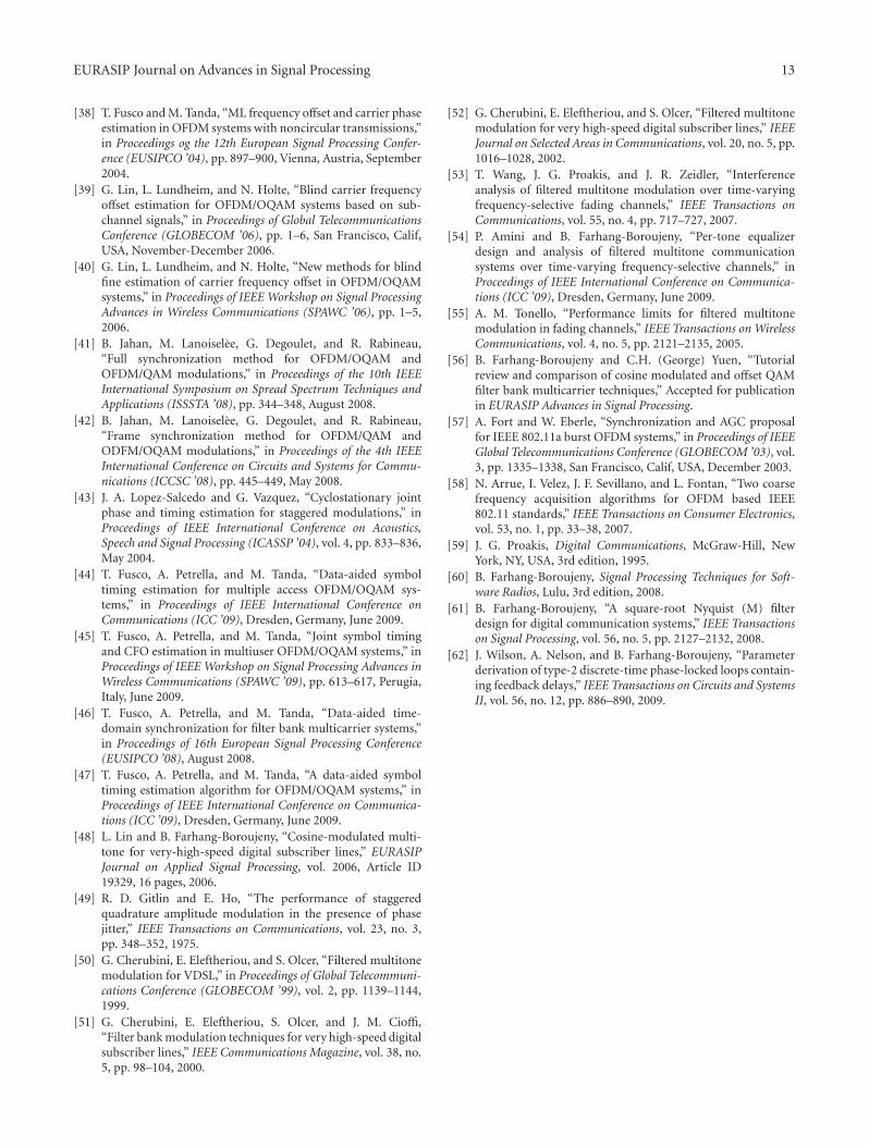
EURASIP Journal on Advances in Signal Processing 13
[38] T. Fusco and M. Tanda, “ML frequency offset and carrier phaseestimation in OFDM systems with noncircular transmissions,”in Proceedings og the 12th European Signal Processing Confer-ence (EUSIPCO ’04), pp. 897–900, Vienna, Austria, September2004.
[39] G. Lin, L. Lundheim, and N. Holte, “Blind carrier frequencyoffset estimation for OFDM/OQAM systems based on sub-channel signals,” in Proceedings of Global TelecommunicationsConference (GLOBECOM ’06), pp. 1–6, San Francisco, Calif,USA, November-December 2006.
[40] G. Lin, L. Lundheim, and N. Holte, “New methods for blindfine estimation of carrier frequency offset in OFDM/OQAMsystems,” in Proceedings of IEEE Workshop on Signal ProcessingAdvances in Wireless Communications (SPAWC ’06), pp. 1–5,2006.
[41] B. Jahan, M. Lanoiselee, G. Degoulet, and R. Rabineau,“Full synchronization method for OFDM/OQAM andOFDM/QAM modulations,” in Proceedings of the 10th IEEEInternational Symposium on Spread Spectrum Techniques andApplications (ISSSTA ’08), pp. 344–348, August 2008.
[42] B. Jahan, M. Lanoiselee, G. Degoulet, and R. Rabineau,“Frame synchronization method for OFDM/QAM andODFM/OQAM modulations,” in Proceedings of the 4th IEEEInternational Conference on Circuits and Systems for Commu-nications (ICCSC ’08), pp. 445–449, May 2008.
[43] J. A. Lopez-Salcedo and G. Vazquez, “Cyclostationary jointphase and timing estimation for staggered modulations,” inProceedings of IEEE International Conference on Acoustics,Speech and Signal Processing (ICASSP ’04), vol. 4, pp. 833–836,May 2004.
[44] T. Fusco, A. Petrella, and M. Tanda, “Data-aided symboltiming estimation for multiple access OFDM/OQAM sys-tems,” in Proceedings of IEEE International Conference onCommunications (ICC ’09), Dresden, Germany, June 2009.
[45] T. Fusco, A. Petrella, and M. Tanda, “Joint symbol timingand CFO estimation in multiuser OFDM/OQAM systems,” inProceedings of IEEE Workshop on Signal Processing Advances inWireless Communications (SPAWC ’09), pp. 613–617, Perugia,Italy, June 2009.
[46] T. Fusco, A. Petrella, and M. Tanda, “Data-aided time-domain synchronization for filter bank multicarrier systems,”in Proceedings of 16th European Signal Processing Conference(EUSIPCO ’08), August 2008.
[47] T. Fusco, A. Petrella, and M. Tanda, “A data-aided symboltiming estimation algorithm for OFDM/OQAM systems,” inProceedings of IEEE International Conference on Communica-tions (ICC ’09), Dresden, Germany, June 2009.
[48] L. Lin and B. Farhang-Boroujeny, “Cosine-modulated multi-tone for very-high-speed digital subscriber lines,” EURASIPJournal on Applied Signal Processing, vol. 2006, Article ID19329, 16 pages, 2006.
[49] R. D. Gitlin and E. Ho, “The performance of staggeredquadrature amplitude modulation in the presence of phasejitter,” IEEE Transactions on Communications, vol. 23, no. 3,pp. 348–352, 1975.
[50] G. Cherubini, E. Eleftheriou, and S. Olcer, “Filtered multitonemodulation for VDSL,” in Proceedings of Global Telecommuni-cations Conference (GLOBECOM ’99), vol. 2, pp. 1139–1144,1999.
[51] G. Cherubini, E. Eleftheriou, S. Olcer, and J. M. Cioffi,“Filter bank modulation techniques for very high-speed digitalsubscriber lines,” IEEE Communications Magazine, vol. 38, no.5, pp. 98–104, 2000.
[52] G. Cherubini, E. Eleftheriou, and S. Olcer, “Filtered multitonemodulation for very high-speed digital subscriber lines,” IEEEJournal on Selected Areas in Communications, vol. 20, no. 5, pp.1016–1028, 2002.
[53] T. Wang, J. G. Proakis, and J. R. Zeidler, “Interferenceanalysis of filtered multitone modulation over time-varyingfrequency-selective fading channels,” IEEE Transactions onCommunications, vol. 55, no. 4, pp. 717–727, 2007.
[54] P. Amini and B. Farhang-Boroujeny, “Per-tone equalizerdesign and analysis of filtered multitone communicationsystems over time-varying frequency-selective channels,” inProceedings of IEEE International Conference on Communica-tions (ICC ’09), Dresden, Germany, June 2009.
[55] A. M. Tonello, “Performance limits for filtered multitonemodulation in fading channels,” IEEE Transactions on WirelessCommunications, vol. 4, no. 5, pp. 2121–2135, 2005.
[56] B. Farhang-Boroujeny and C.H. (George) Yuen, “Tutorialreview and comparison of cosine modulated and offset QAMfilter bank multicarrier techniques,” Accepted for publicationin EURASIP Advances in Signal Processing.
[57] A. Fort and W. Eberle, “Synchronization and AGC proposalfor IEEE 802.11a burst OFDM systems,” in Proceedings of IEEEGlobal Telecommunications Conference (GLOBECOM ’03), vol.3, pp. 1335–1338, San Francisco, Calif, USA, December 2003.
[58] N. Arrue, I. Velez, J. F. Sevillano, and L. Fontan, “Two coarsefrequency acquisition algorithms for OFDM based IEEE802.11 standards,” IEEE Transactions on Consumer Electronics,vol. 53, no. 1, pp. 33–38, 2007.
[59] J. G. Proakis, Digital Communications, McGraw-Hill, NewYork, NY, USA, 3rd edition, 1995.
[60] B. Farhang-Boroujeny, Signal Processing Techniques for Soft-ware Radios, Lulu, 3rd edition, 2008.
[61] B. Farhang-Boroujeny, “A square-root Nyquist (M) filterdesign for digital communication systems,” IEEE Transactionson Signal Processing, vol. 56, no. 5, pp. 2127–2132, 2008.
[62] J. Wilson, A. Nelson, and B. Farhang-Boroujeny, “Parameterderivation of type-2 discrete-time phase-locked loops contain-ing feedback delays,” IEEE Transactions on Circuits and SystemsII, vol. 56, no. 12, pp. 886–890, 2009.
Hindawi Publishing CorporationEURASIP Journal on Advances in Signal ProcessingVolume 2010, Article ID 897607, 11 pagesdoi:10.1155/2010/897607
Research Article
Joint Symbol Timing and CFO Estimation for OFDM/OQAMSystems in Multipath Channels
Tilde Fusco (EURASIP Member),1 Angelo Petrella,2 and Mario Tanda3
1 Communications Regulatory Authority, Department for Studies, Research and Education, Centro Direzionale,Isola B5, 80143 Napoli, Italy
2 Selex Sistemi Integrati, Via Giulio Cesare 268, Bacoli, 80070 Napoli, Italy3 Dipartimento di Ingegneria Biomedica, Elettronica e delle Telecomunicazioni, Universita di Napoli Federico II,Via Claudio 21, 80125 Napoli, Italy
Correspondence should be addressed to Mario Tanda, [email protected]
Received 27 May 2009; Revised 27 September 2009; Accepted 13 November 2009
Academic Editor: Faouzi Bader
Copyright © 2010 Tilde Fusco et al. This is an open access article distributed under the Creative Commons Attribution License,which permits unrestricted use, distribution, and reproduction in any medium, provided the original work is properly cited.
The problem of data-aided synchronization for orthogonal frequency division multiplexing (OFDM) systems based on offsetquadrature amplitude modulation (OQAM) in multipath channels is considered. In particular, the joint maximum-likelihood(ML) estimator for carrier-frequency offset (CFO), amplitudes, phases, and delays, exploiting a short known preamble, is derived.The ML estimators for phases and amplitudes are in closed form. Moreover, under the assumption that the CFO is sufficientlysmall, a closed form approximate ML (AML) CFO estimator is obtained. By exploiting the obtained closed form solutions acost function whose peaks provide an estimate of the delays is derived. In particular, the symbol timing (i.e., the delay of thefirst multipath component) is obtained by considering the smallest estimated delay. The performance of the proposed joint AMLestimator is assessed via computer simulations and compared with that achieved by the joint AML estimator designed for AWGNchannel and that achieved by a previously derived joint estimator for OFDM systems.
1. Introduction
In the last years, the interest for filter-bank multicarrier(FBMC) systems is increased, since they provide highspectral containment. Therefore, they have been taken intoaccount for high-data-rate transmissions over both wiredand wireless frequency-selective channels. Moreover, theyhave been considered for the physical layer of cognitiveradio systems [1]. One of the most famous multicarriermodulation techniques is orthogonal frequency divisionmultiplexing (OFDM), embedded in several standards suchas digital audio and video broadcasting or Wi-Fi wire-less LANs IEEE 802.11a/g. Other known types of FBMCsystems are Filtered Multitone (FMT) systems, that havebeen proposed for very high-speed digital subscriber linestandards [2] and are under investigation also for broadbandwireless applications [3] and, moreover, OFDM based onoffset QAM modulation (OQAM), considered by the 3GPPstandardization forum for improved down-link UTRANinterfaces [4].
Unlike OFDM, OFDM/OQAM systems do not requirethe presence of a cyclic prefix (CP) in order to combatthe effects of frequency selective channels. The absenceof the CP implies on one hand the maximum spectralefficiency and, on the other hand, an increased compu-tational complexity. However, since the subchannel filtersare obtained by complex modulation of a single filter,efficient polyphase implementations are possible. Anotherfundamental difference between OFDM and OFDM/OQAMsystems is the adoption in the latter case of pulse shapingfilters very well localized in time and frequency [5, 6].
OFDM/OQAM systems are more sensitive to synchro-nization errors than single-carrier systems. In particular,carrier frequency-offset (CFO) and symbol timing (ST)estimation errors can lead to a performance degradation.For this reason, it is very important to derive efficientsynchronization schemes. In the last years several studieshave been focused on blind or data-aided synchronizationfor OFDM/OQAM systems. For example, in [7, 8] blindCFO estimators have been derived. Moreover, in [9] a blind
2 EURASIP Journal on Advances in Signal Processing
joint CFO and ST estimator is proposed. Furthermore, in[10] a synchronization scheme for data-aided ST and CFOestimation with robust acquisition properties in dispersivechannels is developed. Finally, in [11, 12] a full synchroniza-tion method utilizing frequency domain scattered pilots inthe time domain is proposed. However, all cited estimatorsare designed for down-link communications.
In this paper we consider the problem of data-aidedsynchronization for OFDM/OQAM systems in multipathchannels. In particular, the joint maximum-likelihood (ML)estimator for CFO, amplitudes, phases, and delays, exploitinga short known preamble, is derived. The ML estimators forphases and amplitudes are in closed form. Moreover, underthe assumption that the CFO is sufficiently small, a closedform approximate ML (AML) CFO estimator is obtained. Byexploiting the obtained closed form solutions a cost functionwhose peaks provide an estimate of the delays is derived.In particular, the ST (i.e., the delay of the first multipathcomponent) is obtained by considering the smallest esti-mated delay. The proposed joint estimator is derived withreference to a down-link scenario; however, by followingan approach similar to that considered in [13], it can beeasily modified to be exploited for up-link communications.The performance of the proposed joint AML estimator isassessed via computer simulations and compared with thatachieved by the joint AML estimator designed for AWGNchannel and that achieved by a previously derived jointestimator for OFDM systems. The paper is organized asfollows. In Section 2 the OFDM/OQAM system model isdescribed. In Section 3 the proposed data-aided estimator isdescribed. In Section 4 numerical results obtained in AWGNand multipath channel are presented and discussed. Finally,conclusions are drawn in Section 5.
Notation 1. j �√−1, superscript (·)∗ denotes the complex
conjugation, R[·] real part, I[·] imaginary part, and | · |absolute value. Moreover, (·)T denotes transpose and ∠[·]the argument of a complex number in [−π,π). Finally, lowercase boldface symbols denote column vectors.
2. System Model
Let us consider an OFDM/OQAM system with N subcarriersin a multipath channel. The received signal, in the presenceof a CFO normalized to subcarrier spacing ε = Δ f T , can bewritten as
r(t) = e j(2π/T)εtNc∑
i=1
γiejφi s(t − τi) + n(t), (1)
where s(t) is the information-bearing signal, Nc is thenumber of multipath components, and, γi, φi, and τi denoteamplitude, phase, and delay, respectively, of the ith path.Moreover, in (1) n(t) is a zero-mean complex-valued whiteGaussian noise process with independent real and imaginarypart, each with two-sided power spectral density σ2
n/2. Thereceived signal r(t) is filtered with an ideal lowpass filter with
a bandwidth of 1/Ts, where Ts denotes the sampling period.The sampled signal s(kTs) is equal to
s(kTs) =√
N
2Nu
S−1∑
p=0
∑
l∈A
e jl((2π/N)k+π/2)
×[aRp,lg
(kTs − pT
)+ jaIp,lg
(kTs − pT − T
2
)],
(2)
where T = NTs is the OFDM/OQAM symbol intervaland S denotes the number of information-bearing symbolsin the burst. Moreover, in (2) A is the set of size Nu ofused subcarriers, aRp,l and aIp,l denote the real and imaginarypart of the complex data symbol transmitted on the lthsubcarrier during the pth OFDM/OQAM symbol, whilethe real-valued and unit-energy pulse-shaping filter g(t) isbandlimited within [−1/T , 1/T].
3. Joint Symbol Timing and CFO Estimator
In this section we consider the problem of data-aidedsynchronization for OFDM/OQAM systems in multipathchannels. In particular, we derive the joint ML estimatorfor CFO, amplitudes, phases, and delays, exploiting a shortknown preamble embedded in the received burst. Specifi-cally, the known preamble is given by
z(kTs) =√
N
2Nu
L−1∑
p=0
∑
l∈P
e jl((2π/T)kTs+π/2)
×[aRp,lg
(kTs − pT
)+ jaIp,lg
(kTs − pT − T
2
)],
(3)
where L is the number of OFDM/OQAM symbols inthe preamble, P is the set of pilot subcarriers, and aRp,l,
aIp,l ∈ {−1, 1}, 0 ≤ p ≤ L − 1, l ∈ P , denote the knownpilot symbols. Note that the duration of the preamble isD = (β + 1/2 + L − 1)T where β is the overlap parameter,that is, the ratio between the length of the truncated pulse-shaping filter and the OFDM/OQAM symbol interval T .By considering an observations window of total length ηNcontaining the nonzero support of the received preamble, thelikelihood function for the unknown parameters ε, and, γi,φi, and τi, i = 1, . . . ,Nc, is given by
Λ(γ, φ, τ, ε
)
=exp
⎧⎪⎨⎪⎩−Tsσ2n
ηN−1∑
k=0
∣∣∣∣∣∣r(kTs)−
Nc∑
i=1
γiejφi zτi,ε(kTs)
∣∣∣∣∣∣
2⎫⎪⎬⎪⎭
,(4)
where γ = [γ1, γ2, . . . , γNc]T , φ = [φ1, φ2, . . . , φNc]
T, τ =
[τ1, τ2, . . . , τNc]T ,
zτ,ε(kTs)Δ= z(kTs − τ)e j(2π/N)εk, (5)
EURASIP Journal on Advances in Signal Processing 3
and the notation of the type x indicates trial value of x. Thus,the log-likelihood function for the parameters of interestresults to be (up to irrelevant factors)
lnΛ(γ, φ, τ, ε
)= −
ηN−1∑
k=0
∣∣∣∣∣∣
Nc∑
i=1
γiejφi zτi ,ε(kTs)
∣∣∣∣∣∣
2
+ 2R
⎡⎣ηN−1∑
k=0
r(kTs)Nc∑
i=1
γie− jφi zτi ,ε(kTs)
∗⎤⎦.
(6)
The first term in the right-hand side (RHS) of (6) for N � 1can be approximated as
ηN−1∑
k=0
∣∣∣∣∣∣
Nc∑
i=1
γiejφi zτi ,ε(kTs)
∣∣∣∣∣∣
2
�Nc∑
i=1
γ2i
ηN−1∑
k=0
|z(kTs − τi)|2. (7)
Therefore, the log-likelihood function can be written as
lnΛ(γ, φ, τ, ε
)=
Nc∑
i=1
{γiR[e− jφi c(τi, ε)
]− γ2
i d(τi)}
, (8)
where
d(τ) =ηN−1∑
k=0
∣∣z(kTs − τ)∣∣2, (9)
c(τ, ε)Δ=∑
l∈P
e− j(π/2)lL−1∑
p=0
[aRp,lw
(l)p (τ, ε)− jaIp,lw
(l)p (τ, ε)
](10)
with
w(l)p (τ, ε)
Δ=√
2NNu
e j(2π/T)τlηN−1∑
k=0
r(kTs)
× g(kTs − pT − τ)e− j(2π/N)k(l+ε),
(11)
w(l)p (τ, ε)
Δ= w(l)p
(τ +
T
2, ε)e− jπl. (12)
From (8), it immediately follows that the ML estimator forphase and amplitude of the ith path is given by
φiML(τi, ε) = arg maxφi
{lnΛ(γ, φ, τ, ε
)}= ∠c(τi, ε), (13)
γiML(τi, ε) = arg maxγi
{lnΛ(γ, φ, τ, ε
)}=∣∣c(τi, ε)
∣∣
2d(τi). (14)
Moreover, by replacing the estimate of the phase and theamplitude of each path in (8) we get
lnΛ(γ(τ, ε), φ(τ, ε), τ, ε
)=
Nc∑
i=1
∣∣c(τi, ε)∣∣2
2d(τi). (15)
Therefore, the joint estimatorfor CFO and delays is given by
(τML, εML) = arg max(τ,ε)
⎧⎨⎩
Nc∑
i=1
|c(τi, ε)|22d(τi)
⎫⎬⎭. (16)
The derived joint ML estimator evaluates, for each trialvalue of each delay τi, i = 1, 2, . . . ,Nc, and for each trialvalue of the CFO ε, the response of the filter matched tothe pulse shaping filter g(·) to the CFO compensated and
downconverted signal r(kTs)e− j(2π/N)εke− j(2π/N)kl at the timeinstants τi + pT and τi + pT + T/2, 0 ≤ p ≤ L − 1.Specifically, the downconversion is performed by consideringall the frequencies of the pilot subcarriers. Then, exploitingthe known pilot symbols, these quantities are combinedaccording to (11) (or (12)), (10), and (16). Note that theproposed algorithm can be exploited also in the up-linkto estimate the desired parameters by considering only thesubcarriers assigned to the user of interest. The joint MLestimate for delays and CFO is obtained by consideringthe value of (τ, ε) that maximizes the statistic in (15).The (Nc + 1)-dimensional maximization required by thejoint ML estimator in (16) undertakes heavy computationalburden. Therefore, in the following is derived a more feasiblesynchronization scheme by exploiting the assumption thatthe CFO is sufficiently small. Specifically, taking into accountthat the observations window contains the nonzero supportof the received preamble and that the prototype filter g(kTs)is different from zero for k ∈ {0,βN−1}, from (11) it followsthat
w(l)p (τ, ε) =
√2NNu
e− j2πεpe− j(2π/N)εθ
×βN−1∑
m=0
r[(m + pN + θ
)Ts]× e− j(2π/N)εm
× g(mTs)e− j(2π/N)ml,
(17)
where the integer θ is the trial value of the delay τ normalized
to the sampling interval, θ = τ/Ts. Then, under theassumption that the CFO is sufficiently small within atime ΔQ comparable with the length of the prototype filtere− j(2π/N)εΔQ � 1, it results that
w(l)p (τ, ε) � e− j2πεpe− j(2π/N)εθul
(pN + θ
), (18)
w(l)p (τ, ε) � e− j2πε(p+(1/2))e− j(2π/N)εθe− jπlul
(pN +
N
2+ θ)
,
(19)
where
ul(k) �βN−1∑
m=0
r[(m + k)Ts]g(mTs)e− j(2π/N)ml. (20)
4 EURASIP Journal on Advances in Signal Processing
In particular, into the case of a training sequence composedof L = 1 OFDM/OQAM symbol, (10), taking into account(18)–(20), becomes
c(τ, ε) =∑
l∈P
e− j(π/2)l[aR0,lw
(l)0 (τ, ε)− jaI0,lw
(l)0 (τ, ε)
]
� A(τ) + e− jπεB(τ)
(21)
with
A(τ)Δ= e− j(2π/N)εθ
∑
l∈P
e− j(π/2)laR0,lul(θ)
, (22)
B(τ)Δ=e− j(2π/N)εθ
∑
l∈P
e− j(π/2)(l+1)aI0,le− jπlul
(N/2+θ
). (23)
Therefore, under the assumption |ε| � N/ΔQ and in thecase of a training sequence with L = 1 OFDM/OQAMsymbol, the AML estimator for CFO, taking into account(16), is given by
εAML(τ) = arg maxε
⎧⎪⎨⎪⎩
Nc∑
i=1
∣∣∣A(τi) + e− jπεB(τi)∣∣∣
2
2d(τi)
⎫⎪⎬⎪⎭
= 1π
∠⎧⎨⎩
Nc∑
i=1
A∗(τi)B(τi)d(τi)
⎫⎬⎭.
(24)
Moreover, from (16) and (21)–(24) it follows that
τAML = arg maxτ
⎧⎨⎩
Nc∑
i=1
[|A(τi)|2 + |B(τi)|2
2d(τi)
]
+
∣∣∣∣∣∣
Nc∑
i=1
A∗(τi)B(τi)d(τi)
∣∣∣∣∣∣
⎫⎬⎭.
(25)
Thus, although under the assumption of small CFO valuesa closed form approximate estimator can be obtained,the estimation of the delays remains an Nc−dimensionalproblem. To simplify the estimation of the delays the lastterm in the RHS of (25) can be neglected, and, then, weobtain
τAML1 = arg maxτ
⎧⎨⎩
Nc∑
i=1
|A(τi)|2 + |B(τi)|22d(τi)
⎫⎬⎭. (26)
In this case, if the number of paths Nc is known, itimmediately follows that theNc-dimensional vector of delaysthat maximize (26) can be obtained by considering the Nc
points where the cost function
MD(τ) = |A(τ)|2 + |B(τ)|2d(τ)
(27)
presents the highest Nc peaks. Moreover, the lowest amongthe obtained delays represents an estimate of the ST. If thenumber of paths Nc is not known in advance, a sufficientlyhigh number of paths should be considered to avoid tolose a strong path and, moreover, to avoid to consider
very weak paths. The obtained delays can be substituted in(24) to obtain the CFO estimate, and, finally, phases andamplitudes can be obtained from (13) and (14), respectively.Note that the numerical results reported in the next sectionshow that the considered approximation of (25) leads to asymbol timing estimator with satisfactory performance if thenumber of subcarriers is sufficiently large.
In Appendix A we analyzed the accuracy of the closedform AML CFO estimator (24) in the absence of noisein a single-path channel and in the case of perfect STsynchronization (Nc = 1 and τ1 = 0 in (1)). Specifically,it is shown that in this case also if the interference fromthe data burst following the training symbol is neglected,the CFO estimator is expected to exhibit a performancefloor. However, it is shown in the next section that thisperformance floor can be substantially reduced if the trainingsymbol satisfies the condition
∑
l∈P
aR0,laI0,l = 0. (28)
Moreover, in Appendix B is derived an approximate expres-sion for the mean square error (MSE) of the AML CFOestimator in (24) for a single-path channel and in the caseof perfect ST synchronization. In particular, in Appendix B itis shown that in this case the MSE can be approximated by
E[
(ε − ε)2]= 2π2NSNR
1∣∣∣∑βN−1
k=0 g(k)2e j(2π/N)εk∣∣∣
2 , (29)
where SNRΔ= γ2/σ2
n and g(k) � g(kTs)/√∑βN−1
l=0 g2(lTs).Note that for ε = 0 the MSE in (29) is coincident with theMSE of the CFO estimator for OFDM systems proposed bySchmidl and Cox (SC) in [14]. It is worthwhile to emphasizethat the MSE in (29) has been derived by neglecting theinterference at the output of each matched filter due toadjacent subcarriers. Therefore, the actual performance ofthe proposed AML CFO estimator presents a floor that is notpredicted by (29). However, it is shown in the next sectionthat the approximate expression in (29) can be exploited inthe range of moderate SNR values.
4. Numerical Results and Comparisons
In this section the performance of the proposed joint AMLestimator is assessed via computer simulations. A numberof 5000 Monte Carlo trials has been performed under thefollowing conditions (unless otherwise stated):
(1) the considered OFDM/OQAM system has a band-width B = 1/Ts = 11.2 MHz;
(2) the data symbols aRp,l and aIp,l are the real andimaginary part of QPSK symbols;
(3) the length of the considered prototype filter(designed with the frequency sampling technique[15]) is LP = βN , where the overlap parameter β isfixed at β = 4;
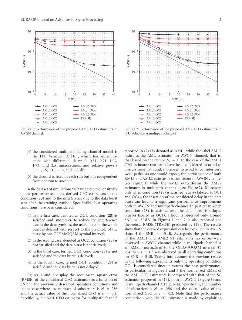
EURASIP Journal on Advances in Signal Processing 5
10−4
10−3
10−2
10−1
0 5 10 15 20 25 30 35 40
RM
SE(ε
)
SNR (dB)
AML1 OC1AML2 OC1AML1 OC2AML2 OC2AML1 OC3
AML2 OC3AML1 OC4AML2 OC4TRMSE
Figure 1: Performance of the proposed AML CFO estimators inAWGN channel.
(4) the considered multipath fading channel model isthe ITU Vehicular A [16], which has six multi-paths with differential delays 0, 0.31, 0.71, 1.09,1.73, and 2.51 microseconds and relative powers0,−1,−9,−10,−15, and −20 dB;
(5) the channel is fixed in each run but it is independentfrom one run to another.
In the first set of simulations we have tested the sensitivityof the performance of the derived CFO estimators to thecondition (28) and to the interference due to the data burstsent after the training symbol. Specifically, four operatingconditions have been considered:
(1) in the first case, denoted as OC1, condition (28) issatisfied and, moreover, to reduce the interferencedue to the data symbols, the useful data in the wholeburst is delayed with respect to the preamble of theburst by one OFDM/OQAM symbol interval;
(2) in the second case, denoted as OC2, condition (28) isnot satisfied and the data burst is not delayed;
(3) in the third case, termed OC3, condition (28) is notsatisfied and the data burst is delayed;
(4) in the fourth case, termed OC4, condition (28) issatisfied and the data burst is not delayed.
Figures 1 and 2 display the root mean square error(RMSE) of the considered CFO estimators as a function ofSNR in the previously described operating conditions andin the case where the number of subcarriers is N = 256and the actual value of the normalized CFO is ε = 0.2.Specifically, the AML CFO estimator for multipath channel
10−4
10−3
10−2
10−1
0 5 10 15 20 25 30 35 40
RM
SE(ε
)
SNR (dB)
AML1 OC1AML2 OC1AML1 OC2AML2 OC2AML1 OC3
AML2 OC3AML1 OC4AML2 OC4TRMSE
Figure 2: Performance of the proposed AML CFO estimators inITU Vehicular A multipath channel.
reported in (24) is denoted as AML1 while the label AML2indicates the AML estimator for AWGN channel, that is,that based on the choice Nc = 1. In the case of the AML1CFO estimator two paths have been considered to avoid tolose a strong path and, moreover, to avoid to consider veryweak paths. As one would expect, the performance of bothAML1 and AML2 estimators is coincident in AWGN channel(see Figure 1) while the AML1 outperforms the AML2estimator in multipath channel (see Figure 2). Moreover,only when condition (28) is satisfied (curves labeled as OC1and OC4), the insertion of the considered delay in the databurst can lead to a significant performance improvementboth in AWGN and multipath channel. In particular, whencondition (28) is satisfied and the data burst is delayed(curves labeled as OC1), a floor is observed only aroundSNR = 30 dB. In Figures 1 and 2 is also reported thetheoretical RMSE (TRMSE) predicted by (29). The resultsshow that the derived expression can be exploited in AWGNchannel for SNR ≤ 15 dB. As regards the performanceof the AML1 and AML2 ST estimators no errors wereobserved in AWGN channel while in multipath channel Aan RMSE (normalized to the OFDM/OQAM interval T)less than 3 · 10−3 was observed in all operating conditionsfor SNR ≥ 5 dB. Taking into account the previous resultsin the following experiments only the operating conditionOC1 is considered since it assures the best performance.In particular, in Figures 3 and 4 the normalized RMSE ofthe AML CFO estimators is compared with that of the SCestimator proposed in [14], both in AWGN (Figure 3) andin multipath channel A (Figure 4). Specifically, the numberof subcarriers is N = 256 and the actual value of thenormalized CFO is ε = 0.2. Note that the performancecomparison with the SC estimator is made by exploiting
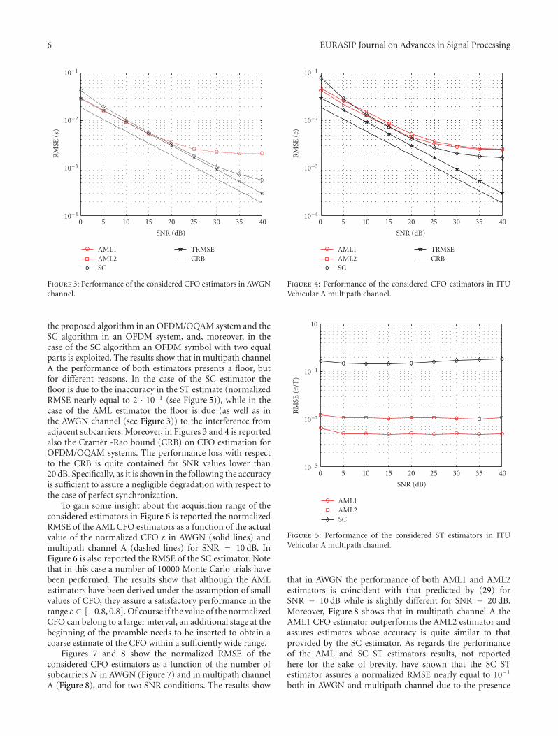
6 EURASIP Journal on Advances in Signal Processing
10−4
10−3
10−2
10−1
0 5 10 15 20 25 30 35 40
RM
SE(ε
)
SNR (dB)
AML1AML2SC
TRMSECRB
Figure 3: Performance of the considered CFO estimators in AWGNchannel.
the proposed algorithm in an OFDM/OQAM system and theSC algorithm in an OFDM system, and, moreover, in thecase of the SC algorithm an OFDM symbol with two equalparts is exploited. The results show that in multipath channelA the performance of both estimators presents a floor, butfor different reasons. In the case of the SC estimator thefloor is due to the inaccuracy in the ST estimate (normalizedRMSE nearly equal to 2 · 10−1 (see Figure 5)), while in thecase of the AML estimator the floor is due (as well as inthe AWGN channel (see Figure 3)) to the interference fromadjacent subcarriers. Moreover, in Figures 3 and 4 is reportedalso the Cramer -Rao bound (CRB) on CFO estimation forOFDM/OQAM systems. The performance loss with respectto the CRB is quite contained for SNR values lower than20 dB. Specifically, as it is shown in the following the accuracyis sufficient to assure a negligible degradation with respect tothe case of perfect synchronization.
To gain some insight about the acquisition range of theconsidered estimators in Figure 6 is reported the normalizedRMSE of the AML CFO estimators as a function of the actualvalue of the normalized CFO ε in AWGN (solid lines) andmultipath channel A (dashed lines) for SNR = 10 dB. InFigure 6 is also reported the RMSE of the SC estimator. Notethat in this case a number of 10000 Monte Carlo trials havebeen performed. The results show that although the AMLestimators have been derived under the assumption of smallvalues of CFO, they assure a satisfactory performance in therange ε ∈ [−0.8, 0.8]. Of course if the value of the normalizedCFO can belong to a larger interval, an additional stage at thebeginning of the preamble needs to be inserted to obtain acoarse estimate of the CFO within a sufficiently wide range.
Figures 7 and 8 show the normalized RMSE of theconsidered CFO estimators as a function of the number ofsubcarriers N in AWGN (Figure 7) and in multipath channelA (Figure 8), and for two SNR conditions. The results show
10−4
10−3
10−2
10−1
0 5 10 15 20 25 30 35 40
RM
SE(ε
)
SNR (dB)
AML1AML2SC
TRMSECRB
Figure 4: Performance of the considered CFO estimators in ITUVehicular A multipath channel.
10−3
10−2
10−1
10
0 5 10 15 20 25 30 35 40
RM
SE(τ
/T)
SNR (dB)
AML1AML2SC
Figure 5: Performance of the considered ST estimators in ITUVehicular A multipath channel.
that in AWGN the performance of both AML1 and AML2estimators is coincident with that predicted by (29) forSNR = 10 dB while is slightly different for SNR = 20 dB.Moreover, Figure 8 shows that in multipath channel A theAML1 CFO estimator outperforms the AML2 estimator andassures estimates whose accuracy is quite similar to thatprovided by the SC estimator. As regards the performanceof the AML and SC ST estimators results, not reportedhere for the sake of brevity, have shown that the SC STestimator assures a normalized RMSE nearly equal to 10−1
both in AWGN and multipath channel due to the presence
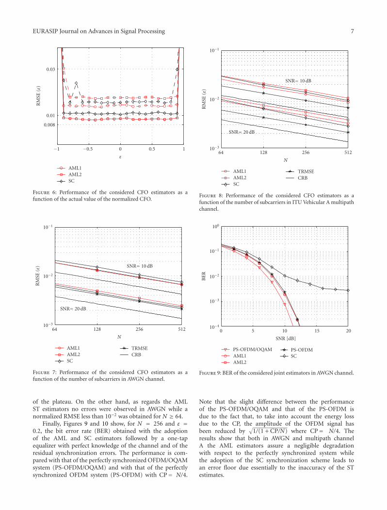
EURASIP Journal on Advances in Signal Processing 7
0.008
0.01
0.03
−1 −0.5 0 0.5 1
RM
SE(ε
)
ε
AML1AML2SC
Figure 6: Performance of the considered CFO estimators as afunction of the actual value of the normalized CFO.
10−3
10−2
10−1
SNR= 20 dB
64 128
SNR= 10 dB
256 512
RM
SE(ε
)
N
AML1AML2SC
TRMSECRB
Figure 7: Performance of the considered CFO estimators as afunction of the number of subcarriers in AWGN channel.
of the plateau. On the other hand, as regards the AMLST estimators no errors were observed in AWGN while anormalized RMSE less than 10−2 was obtained for N ≥ 64.
Finally, Figures 9 and 10 show, for N = 256 and ε =0.2, the bit error rate (BER) obtained with the adoptionof the AML and SC estimators followed by a one-tapequalizer with perfect knowledge of the channel and of theresidual synchronization errors. The performance is com-pared with that of the perfectly synchronized OFDM/OQAMsystem (PS-OFDM/OQAM) and with that of the perfectlysynchronized OFDM system (PS-OFDM) with CP= N/4.
10−3
10−2
10−1
SNR= 20 dB
64 128
SNR= 10 dB
256 512
RM
SE(ε
)
N
AML1AML2SC
TRMSECRB
Figure 8: Performance of the considered CFO estimators as afunction of the number of subcarriers in ITU Vehicular A multipathchannel.
10−4
10−3
10−1
10−2
100
0 5 1510 20
BE
R
SNR [dB]
PS-OFDM/OQAMAML1AML2
PS-OFDMSC
Figure 9: BER of the considered joint estimators in AWGN channel.
Note that the slight difference between the performanceof the PS-OFDM/OQAM and that of the PS-OFDM isdue to the fact that, to take into account the energy lossdue to the CP, the amplitude of the OFDM signal hasbeen reduced by
√1/(1 + CP/N) where CP= N/4. The
results show that both in AWGN and multipath channelA the AML estimators assure a negligible degradationwith respect to the perfectly synchronized system whilethe adoption of the SC synchronization scheme leads toan error floor due essentially to the inaccuracy of the STestimates.
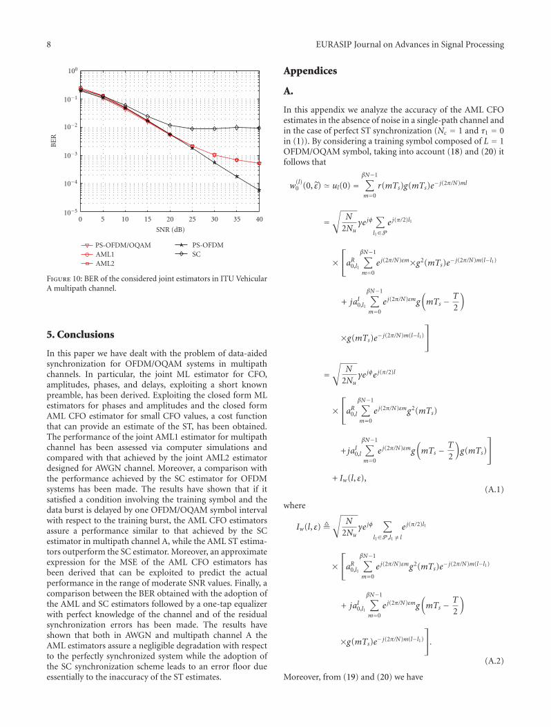
8 EURASIP Journal on Advances in Signal Processing
10−5
10−4
10−3
100
10−2
10−1
0 5 10 15 20 25 30 35 40
BE
R
SNR (dB)
PS-OFDM/OQAMAML1AML2
PS-OFDMSC
Figure 10: BER of the considered joint estimators in ITU VehicularA multipath channel.
5. Conclusions
In this paper we have dealt with the problem of data-aidedsynchronization for OFDM/OQAM systems in multipathchannels. In particular, the joint ML estimator for CFO,amplitudes, phases, and delays, exploiting a short knownpreamble, has been derived. Exploiting the closed form MLestimators for phases and amplitudes and the closed formAML CFO estimator for small CFO values, a cost functionthat can provide an estimate of the ST, has been obtained.The performance of the joint AML1 estimator for multipathchannel has been assessed via computer simulations andcompared with that achieved by the joint AML2 estimatordesigned for AWGN channel. Moreover, a comparison withthe performance achieved by the SC estimator for OFDMsystems has been made. The results have shown that if itsatisfied a condition involving the training symbol and thedata burst is delayed by one OFDM/OQAM symbol intervalwith respect to the training burst, the AML CFO estimatorsassure a performance similar to that achieved by the SCestimator in multipath channel A, while the AML ST estima-tors outperform the SC estimator. Moreover, an approximateexpression for the MSE of the AML CFO estimators hasbeen derived that can be exploited to predict the actualperformance in the range of moderate SNR values. Finally, acomparison between the BER obtained with the adoption ofthe AML and SC estimators followed by a one-tap equalizerwith perfect knowledge of the channel and of the residualsynchronization errors has been made. The results haveshown that both in AWGN and multipath channel A theAML estimators assure a negligible degradation with respectto the perfectly synchronized system while the adoption ofthe SC synchronization scheme leads to an error floor dueessentially to the inaccuracy of the ST estimates.
Appendices
A.
In this appendix we analyze the accuracy of the AML CFOestimates in the absence of noise in a single-path channel andin the case of perfect ST synchronization (Nc = 1 and τ1 = 0in (1)). By considering a training symbol composed of L = 1OFDM/OQAM symbol, taking into account (18) and (20) itfollows that
w(l)0 (0, ε) � ul(0) =
βN−1∑
m=0
r(mTs)g(mTs)e− j(2π/N)ml
=√
N
2Nuγe jφ
∑
l1∈P
e j(π/2)l1
×⎡⎣aR0,l1
βN−1∑
m=0
e j(2π/N)εm×g2(mTs)e− j(2π/N)m(l−l1)
+ jaI0,l1
βN−1∑
m=0
e j(2π/N)εmg(mTs − T
2
)
×g(mTs)e− j(2π/N)m(l−l1)
⎤⎦
=√
N
2Nuγe jφe j(π/2)l
×⎡⎣aR0,l
βN−1∑
m=0
e j(2π/N)εmg2(mTs)
+ jaI0,l
βN−1∑
m=0
e j(2π/N)εmg(mTs − T
2
)g(mTs)
⎤⎦
+ Iw(l, ε),(A.1)
where
Iw(l, ε) �√
N
2Nuγe jφ
∑
l1∈P ,l1 /= le j(π/2)l1
×⎡⎣aR0,l1
βN−1∑
m=0
e j(2π/N)εmg2(mTs)e− j(2π/N)m(l−l1)
+ jaI0,l1
βN−1∑
m=0
e j(2π/N)εmg(mTs − T
2
)
×g(mTs)e− j(2π/N)m(l−l1)
⎤⎦.
(A.2)
Moreover, from (19) and (20) we have
EURASIP Journal on Advances in Signal Processing 9
w(l)0 (0, ε) � e− jπεe− jπlul
(N
2
)
= e− jπεe− jπlβN−1∑
m=0
r[(m +
N
2
)Ts
]g(mTs)e− j(2π/N)ml
=√
N
2Nuγe jφe− jπεe− jπl
∑
l1∈P
e j(3π/2)l1
×⎡⎣aR0,l1
βN−1∑
m=0
e j(2π/N)ε(m+(N/2))g(mTs+
T
2
)
× g(mTs)e− j(2π/N)m(l−l1) + jaI0,l1
×βN−1∑
m=0
e j(2π/N)ε(m+(N/2))g2(mTs)e− j(2π/N)m(l−l1)
⎤⎦
=√
N
2Nuγe jφe− jπεe j(π/2)le jπε
×⎡⎣aR0,l
βN−1∑
m=0
e j(2π/N)εmg(mTs +
T
2
)g(mTs)
+ jaI0,l
βN−1∑
m=0
e j(2π/N)εmg2(mTs)
⎤⎦
+ e− jπεe− jπlIw(l, ε),(A.3)
where
Iw(l, ε) �√
N
2Nuγe jφe jπε
∑
l1∈P ,l1 /= le j(3π/2)l1
×⎡⎣aR0,l1
βN−1∑
m=0
e j(2π/N)εm
× g(mTs +
T
2
)g(mTs)e− j(2π/N)m(l−l1)
+ jaI0,l1
βN−1∑
m=0
e j(2π/N)εmg2(mTs)e− j(2π/N)m(l−l1)
⎤⎦.
(A.4)
Therefore, taking into account (18), (20), (22), and (A.1) itfollows that
A(0) =∑
l∈P
e− j(π/2)laR0,lw(l)0 (0, ε) =
√N
2Nuγe jφ
×⎡⎣∑
l∈P
(aR0,l
)2βN−1∑
m=0
e j(2π/N)εmg2(mTs)
+ j∑
l∈P
aR0,laI0,l
βN−1∑
m=0
e j(2π/N)εmg(mTs − T
2
)g(mTs)
⎤⎦
+∑
l∈P
e− j(π/2)laR0,lIw(l, ε).
(A.5)
Moreover, from (19), (20), (23), and (A.3) we have
B(0) = − je jπε∑
l∈P
e− j(π/2)laI0,lw(l)0 (0, ε)
= − j√
N
2Nuγe jφe jπε
×⎡⎣ j∑
l∈P
(aI0,l
)2βN−1∑
m=0
e j(2π/N)εmg2(mTs)
+∑
l∈P
aR0,laI0,l
βN−1∑
m=0
e j(2π/N)εmg(mTs +
T
2
)g(mTs)
⎤⎦
− j∑
l∈P
e− j(3π/2)laI0,lIw(l, ε).
(A.6)
Note that if the training symbol satisfies the condition
∑
l∈P
aR0,laI0,l = 0, (A.7)
it follows that
A(0) =√
N
2Nuγe jφ
∑
l∈P
(aR0,l
)2βN−1∑
m=0
e j(2π/N)εmg2(mTs)
+∑
l∈P
e− j(π/2)laR0,lIw(l, ε),
(A.8)
B(0) = e jπε√
N
2Nuγe jφ
∑
l∈P
(aI0,l
)2βN−1∑
m=0
e j(2π/N)εmg2(mTs)
+∑
l∈P
e− j(π/2)(1+3l)aI0,lIw(l, ε).
(A.9)
In this case, if the interference terms∑
l∈P e− j(π/2)laR0,lIw(l, ε)and
∑l∈P e− j(π/2)(1+3l)aI0,lIw(l, ε) in the RHS of (A.8) and
(A.9), respectively, were negligible, the CFO estimate wouldbe (see (24) for Nc = 1) (1/π)∠{A∗(0)B(0)} = ε. Thepresence of the interference terms in the RHS of (A.8) and(A.9) leads to an error floor. Moreover, if condition (A.7)is not fulfilled an error floor can be observed also whenthe interference terms are negligible (see (A.5) and (A.6)).However, in the section on numerical results it is shown thatthe error floor can be substantially reduced when condition(A.7) is satisfied.
B.
In this appendix we derive an approximate expression for theMSE of the AML CFO estimator reported in (24) for a single-path channel and in the case of perfect ST synchronization(Nc = 1 and τ1 = 0 in (1)). Specifically, we consider the casewhere the SNR is such that interference terms in (A.8) and(A.9) can be neglected with respect to the noise terms dueto AWGN but it is sufficiently high that noise × noise terms
10 EURASIP Journal on Advances in Signal Processing
can be deleted. In this case taking into account (A.1), (A.3),(A.8), and (A.9) it follows that
A∗(0)B(0) � [A∗0 (0) +W∗A
][B0(0) +WB],
� A∗0 (0)B0(0) + A∗0 (0)WB + B0(0)W∗A ,
(B.1)
where the last approximation has been obtained by neglect-ing the noise × noise term, and, moreover, A0(0) and B0(0)represent the contribution to A(0) and B(0) (in (A.8) and(A.9), resp.) in the absence of noise and of the interferenceterms. The noise contributions in (B.1) are given by
WA �βN−1∑
k=0
n(kTs)g(kTs)∑
l∈P
aI0,Re− j(π/2)le− j(2π/N)kl, (B.2)
WB � − jβN−1∑
k=0
n[(k +
N
2
)Ts
]
× g(kTs)∑
l∈P
aI0,I e− j(π/2)le− jπle− j(2π/N)kl,
(B.3)
where the zero-mean circular noise n(kTs) has a varianceE[|n(kTs)|2] = σ2
n/Ts. In this case we obtain
ε − ε = 1π
∠{A∗(0)B(0)e− jπε
}
� 1π
I{e− jπεA∗0 (0)WB + e− jπεB0(0)W∗
A
}
R{A∗0 (0)B0(0)
}
= 1π
I{Z}(N/2Nu)γ2
∑l∈P
(aR0,l
)2∑l∈P
(aI0,l
)2q
= 1π
I{Z}(N/2)γ2Nu
∣∣∣∑βN−1
k=0 e j(2π/N)εkg2(kTs)∣∣∣
2 ,
(B.4)
where q denotes |∑βN−1k=0 e j(2π/N)εkg2(kTs)|
2and the last
equality has been obtained by exploiting the fact that aRp,l,
aIp,l ∈ {−1, 1}, and, moreover,
ZΔ= e− jπεA∗0 (0)WB + e− jπεB0(0)W∗
A . (B.5)
Thus, from (B.4) we obtain
E[
(ε − ε)2]� 1
2π2
E[|Z|2
]−R{E[Z2]}
[(N/2)γ2Nu
∣∣∣∑βN−1
k=0 e j(2π/N)εkg2(kTs)∣∣∣
2]2 .
(B.6)
Finally, under the assumption∑
l∈P aR0,laI0,l±1 � 0, exploiting
the condition (A.7) and the noise circularity, we have
R{E[Z2]} � 0, (B.7)
E[|Z|2]= σ2
n
Ts
βN−1∑
k=0
g2(kTs)Nγ2N2u
∣∣∣∣∣∣
βN−1∑
k=0
e j(2π/N)εkg2(kTs)
∣∣∣∣∣∣
2
.
(B.8)
Therefore, we can write
E[
(ε−ε)2]� 2π2NSNR
1∣∣∣∑βN−1
k=0 g(k)2e j(2π/N)εk∣∣∣
2 , (B.9)
where SNRΔ= γ2/σ2
n and g(k)Δ= g(kTs)
√∑βN−1l=0 g2(lTs).
Acknowledgment
This work was supported in part by the European Commis-sion under Project PHYDYAS (FP7-ICT-2007-1-211887).
References
[1] B. Farhang-Boroujeny and R. Kempter, “Multicarrier commu-nication techniques for spectrum sensing and communicationin cognitive radios,” IEEE Communications Magazine, vol. 46,no. 4, pp. 80–85, 2008.
[2] G. Cherubini, E. Eleftheriou, S. Oker, and J. M. Cioffi,“Filter bank modulation techniques for very high-speed digitalsubscriber lines,” IEEE Communications Magazine, vol. 38, no.5, pp. 98–104, 2000.
[3] T. Ihalainen, T. H. Stitz, M. Rinne, and M. Renfors, “Channelequalization in filter bank based multicarrier modulation forwireless communications,” EURASIP Journal on Advances inSignal Processing, vol. 2007, Article ID 49389, 18 pages, 2007.
[4] D. Lacroix, N. Goudard, and M. Alard, “OFDM with guardinterval versus OFDM/OffsetQAM for high data rate UMTSdownlink transmission,” in Proceedings of the 54th IEEEVehicular Technology Conference (VTC ’01), vol. 4, pp. 2682–2686, Atlantic City, NJ, USA, October 2001.
[5] C. R. M. Alard and P. Siohan, “A family of extended gaussianfunctions with a nearly optimal localization,” in Proceedingsof the 1st International Workshop on Multi-Carrier Spread-Spectrum, pp. 179–186, Oberpfaffenhofen, Germany, April1997.
[6] R. Haas and J.-C. Belfiore, “A time-frequency well-localizedpulse for multiple carrier transmission,” Wireless PersonalCommunications, vol. 5, no. 1, pp. 1–18, 1997.
[7] P. Ciblat and E. Serpedin, “A fine blind frequency offsetestimator for OFDM/OQAM systems,” IEEE Transactions onSignal Processing, vol. 52, no. 1, pp. 291–296, 2004.
[8] T. Fusco and M. Tanda, “Blind frequency-offset estimationfor OFDM/OQAM systems,” IEEE Transactions on SignalProcessing, vol. 55, no. 5, pp. 1828–1838, 2007.
[9] H. Bolcskei, “Blind estimation of symbol timing and carrierfrequency offset in wireless OFDM systems,” IEEE Transactionson Communications, vol. 49, no. 6, pp. 988–999, 2001.
[10] T. Fusco, A. Petrella, and M. Tanda, “Data-aided symboltiming and cfo synchronization for filter-bank multicarriersystems,” IEEE Transactions on Wireless Communications, vol.8, no. 5, pp. 2705–2715, 2009.
EURASIP Journal on Advances in Signal Processing 11
[11] B. Jahan, M. Lanoiselee, G. Degoulet, and R. Rabineau,“Full synchronization method for OFDM/OQAM andOFDM/QAM modulations,” in Proceedings of the 10th IEEEInternational Symposium on Spread Spectrum Techniques andApplications (ISSSTA ’08), pp. 344–348, August 2008.
[12] B. Jahan, M. Lanoiselee, G. Degoulet, and R. Rabineau,“Frame synchronization method for OFDM/QAM andODFM/OQAM modulations,” in Proceedings of the 4th IEEEInternational Conference on Circuits and Systems for Communi-cations (ICCSC ’08), pp. 445–449, Shanghai, China, May 2008.
[13] T. Fusco, A. Petrella, and M. Tanda, “Joint symbol timingand CFO estimation in multiuser OFDM/OQAM systems,”in Proceedings of the 10th IEEE Workshop on Signal ProcessingAdvances in Wireless Communications (SPAWC ’09), pp. 613–617, Perugia, Italy, June 2009.
[14] T. M. Schmidl and D. C. Cox, “Robust frequency andtiming synchronization for OFDM,” IEEE Transactions onCommunications, vol. 45, no. 12, pp. 1613–1621, 1997.
[15] M. G. Bellanger, “Specification and design of a prototype filterfor filter bank based multicarrier transmission,” in Proceedingsof the IEEE International Conference on Acoustics, Speech, andSignal Processing (ICASSP ’01), vol. 4, pp. 2417–2420, SaltLake, Utah, USA, May 2001.
[16] Recommendation ITU-R M. 1225, “Guidelines for evaluationof radio transmission technologies for IMT-2000,” 1997.
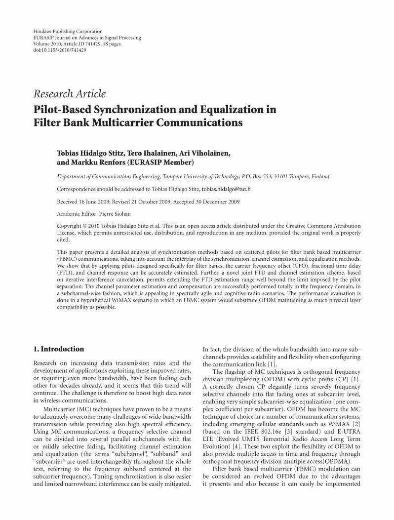
Hindawi Publishing CorporationEURASIP Journal on Advances in Signal ProcessingVolume 2010, Article ID 741429, 18 pagesdoi:10.1155/2010/741429
Research Article
Pilot-Based Synchronization and Equalization inFilter Bank Multicarrier Communications
Tobias Hidalgo Stitz, Tero Ihalainen, Ari Viholainen,and Markku Renfors (EURASIP Member)
Department of Communications Engineering, Tampere University of Technology, P.O. Box 553, 33101 Tampere, Finland
Correspondence should be addressed to Tobias Hidalgo Stitz, [email protected]
Received 16 June 2009; Revised 21 October 2009; Accepted 30 December 2009
Academic Editor: Pierre Siohan
Copyright © 2010 Tobias Hidalgo Stitz et al. This is an open access article distributed under the Creative Commons AttributionLicense, which permits unrestricted use, distribution, and reproduction in any medium, provided the original work is properlycited.
This paper presents a detailed analysis of synchronization methods based on scattered pilots for filter bank based multicarrier(FBMC) communications, taking into account the interplay of the synchronization, channel estimation, and equalization methods.We show that by applying pilots designed specifically for filter banks, the carrier frequency offset (CFO), fractional time delay(FTD), and channel response can be accurately estimated. Further, a novel joint FTD and channel estimation scheme, basedon iterative interference cancelation, permits extending the FTD estimation range well beyond the limit imposed by the pilotseparation. The channel parameter estimation and compensation are successfully performed totally in the frequency domain, ina subchannel-wise fashion, which is appealing in spectrally agile and cognitive radio scenarios. The performance evaluation isdone in a hypothetical WiMAX scenario in which an FBMC system would substitute OFDM maintaining as much physical layercompatibility as possible.
1. Introduction
Research on increasing data transmission rates and thedevelopment of applications exploiting these improved rates,or requiring even more bandwidth, have been fueling eachother for decades already, and it seems that this trend willcontinue. The challenge is therefore to boost high data ratesin wireless communications.
Multicarrier (MC) techniques have proven to be a meansto adequately overcome many challenges of wide bandwidthtransmission while providing also high spectral efficiency.Using MC communications, a frequency selective channelcan be divided into several parallel subchannels with flator mildly selective fading, facilitating channel estimationand equalization (the terms “subchannel”, “subband” and“subcarrier” are used interchangeably throughout the wholetext, referring to the frequency subband centered at thesubcarrier frequency). Timing synchronization is also easierand limited narrowband interference can be easily mitigated.
In fact, the division of the whole bandwidth into many sub-channels provides scalability and flexibility when configuringthe communication link [1].
The flagship of MC techniques is orthogonal frequencydivision multiplexing (OFDM) with cyclic prefix (CP) [1].A correctly chosen CP elegantly turns severely frequencyselective channels into flat fading ones at subcarrier level,enabling very simple subcarrier-wise equalization (one com-plex coefficient per subcarrier). OFDM has become the MCtechnique of choice in a number of communication systems,including emerging cellular standards such as WiMAX [2](based on the IEEE 802.16e [3] standard) and E-UTRALTE (Evolved UMTS Terrestrial Radio Access Long TermEvolution) [4]. These two exploit the flexibility of OFDM toalso provide multiple access in time and frequency throughorthogonal frequency division multiple access(OFDMA).
Filter bank based multicarrier (FBMC) modulation canbe considered an evolved OFDM due to the advantagesit presents and also because it can easily be implemented
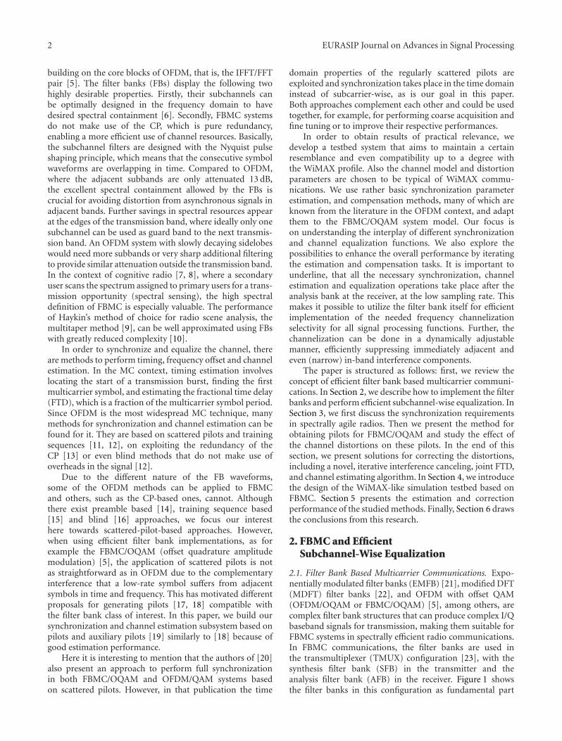
2 EURASIP Journal on Advances in Signal Processing
building on the core blocks of OFDM, that is, the IFFT/FFTpair [5]. The filter banks (FBs) display the following twohighly desirable properties. Firstly, their subchannels canbe optimally designed in the frequency domain to havedesired spectral containment [6]. Secondly, FBMC systemsdo not make use of the CP, which is pure redundancy,enabling a more efficient use of channel resources. Basically,the subchannel filters are designed with the Nyquist pulseshaping principle, which means that the consecutive symbolwaveforms are overlapping in time. Compared to OFDM,where the adjacent subbands are only attenuated 13 dB,the excellent spectral containment allowed by the FBs iscrucial for avoiding distortion from asynchronous signals inadjacent bands. Further savings in spectral resources appearat the edges of the transmission band, where ideally only onesubchannel can be used as guard band to the next transmis-sion band. An OFDM system with slowly decaying sidelobeswould need more subbands or very sharp additional filteringto provide similar attenuation outside the transmission band.In the context of cognitive radio [7, 8], where a secondaryuser scans the spectrum assigned to primary users for a trans-mission opportunity (spectral sensing), the high spectraldefinition of FBMC is especially valuable. The performanceof Haykin’s method of choice for radio scene analysis, themultitaper method [9], can be well approximated using FBswith greatly reduced complexity [10].
In order to synchronize and equalize the channel, thereare methods to perform timing, frequency offset and channelestimation. In the MC context, timing estimation involveslocating the start of a transmission burst, finding the firstmulticarrier symbol, and estimating the fractional time delay(FTD), which is a fraction of the multicarrier symbol period.Since OFDM is the most widespread MC technique, manymethods for synchronization and channel estimation can befound for it. They are based on scattered pilots and trainingsequences [11, 12], on exploiting the redundancy of theCP [13] or even blind methods that do not make use ofoverheads in the signal [12].
Due to the different nature of the FB waveforms,some of the OFDM methods can be applied to FBMCand others, such as the CP-based ones, cannot. Althoughthere exist preamble based [14], training sequence based[15] and blind [16] approaches, we focus our interesthere towards scattered-pilot-based approaches. However,when using efficient filter bank implementations, as forexample the FBMC/OQAM (offset quadrature amplitudemodulation) [5], the application of scattered pilots is notas straightforward as in OFDM due to the complementaryinterference that a low-rate symbol suffers from adjacentsymbols in time and frequency. This has motivated differentproposals for generating pilots [17, 18] compatible withthe filter bank class of interest. In this paper, we build oursynchronization and channel estimation subsystem based onpilots and auxiliary pilots [19] similarly to [18] because ofgood estimation performance.
Here it is interesting to mention that the authors of [20]also present an approach to perform full synchronizationin both FBMC/OQAM and OFDM/QAM systems basedon scattered pilots. However, in that publication the time
domain properties of the regularly scattered pilots areexploited and synchronization takes place in the time domaininstead of subcarrier-wise, as is our goal in this paper.Both approaches complement each other and could be usedtogether, for example, for performing coarse acquisition andfine tuning or to improve their respective performances.
In order to obtain results of practical relevance, wedevelop a testbed system that aims to maintain a certainresemblance and even compatibility up to a degree withthe WiMAX profile. Also the channel model and distortionparameters are chosen to be typical of WiMAX commu-nications. We use rather basic synchronization parameterestimation, and compensation methods, many of which areknown from the literature in the OFDM context, and adaptthem to the FBMC/OQAM system model. Our focus ison understanding the interplay of different synchronizationand channel equalization functions. We also explore thepossibilities to enhance the overall performance by iteratingthe estimation and compensation tasks. It is important tounderline, that all the necessary synchronization, channelestimation and equalization operations take place after theanalysis bank at the receiver, at the low sampling rate. Thismakes it possible to utilize the filter bank itself for efficientimplementation of the needed frequency channelizationselectivity for all signal processing functions. Further, thechannelization can be done in a dynamically adjustablemanner, efficiently suppressing immediately adjacent andeven (narrow) in-band interference components.
The paper is structured as follows: first, we review theconcept of efficient filter bank based multicarrier communi-cations. In Section 2, we describe how to implement the filterbanks and perform efficient subchannel-wise equalization. InSection 3, we first discuss the synchronization requirementsin spectrally agile radios. Then we present the method forobtaining pilots for FBMC/OQAM and study the effect ofthe channel distortions on these pilots. In the end of thissection, we present solutions for correcting the distortions,including a novel, iterative interference canceling, joint FTD,and channel estimating algorithm. In Section 4, we introducethe design of the WiMAX-like simulation testbed based onFBMC. Section 5 presents the estimation and correctionperformance of the studied methods. Finally, Section 6 drawsthe conclusions from this research.
2. FBMC and EfficientSubchannel-Wise Equalization
2.1. Filter Bank Based Multicarrier Communications. Expo-nentially modulated filter banks (EMFB) [21], modified DFT(MDFT) filter banks [22], and OFDM with offset QAM(OFDM/OQAM or FBMC/OQAM) [5], among others, arecomplex filter bank structures that can produce complex I/Qbaseband signals for transmission, making them suitable forFBMC systems in spectrally efficient radio communications.In FBMC communications, the filter banks are used inthe transmultiplexer (TMUX) configuration [23], with thesynthesis filter bank (SFB) in the transmitter and theanalysis filter bank (AFB) in the receiver. Figure 1 showsthe filter banks in this configuration as fundamental part
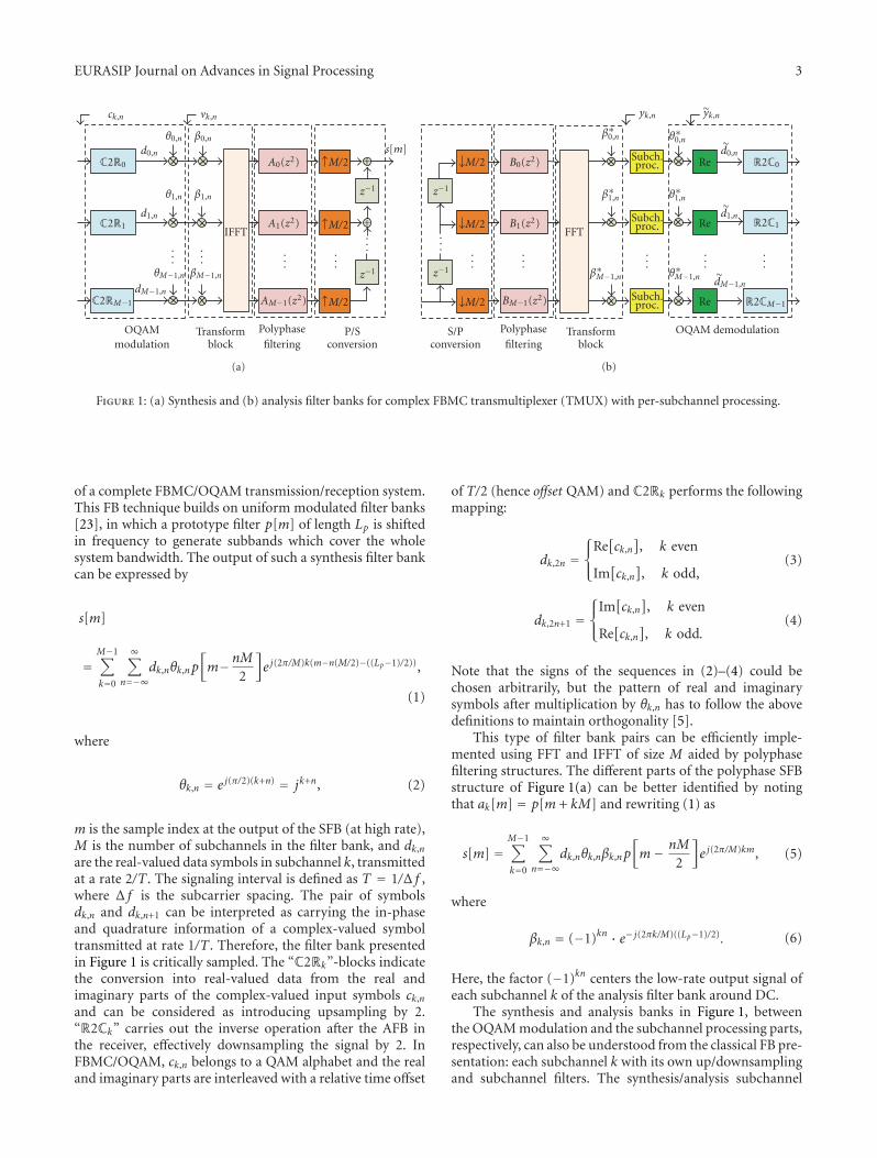
EURASIP Journal on Advances in Signal Processing 3
s[m]C2R0
C2R1
C2RM−1
d0,n
d1,n
dM−1,n
θ0,n
θ1,n
......
θM−1,n
β0,n
β1,n
βM−1,n
...
IFFT
A0(z2)
A1(z2)
AM−1(z2)
M/2
M/2
M/2
...
...
z−1
z−1
+
+
OQAMmodulation
Transformblock
Polyphasefiltering
P/Sconversion
ck,n vk,n
(a)
Re
Re
Re
R2C0
R2C1
R2CM−1
d0,n
d1,n
dM−1,n
θ∗0,n
θ∗1,n
......
... ......
...θ∗M−1,n
β∗0,n
β∗1,n
β∗M−1,n
FFT
B0(z2)
B1(z2)
BM−1(z2)
M/2
M/2
M/2
z−1
z−1
OQAM demodulationTransformblock
Polyphasefiltering
S/Pconversion
yk,n yk,n
Subch.proc.
Subch.proc.
Subch.proc.
(b)
Figure 1: (a) Synthesis and (b) analysis filter banks for complex FBMC transmultiplexer (TMUX) with per-subchannel processing.
of a complete FBMC/OQAM transmission/reception system.This FB technique builds on uniform modulated filter banks[23], in which a prototype filter p[m] of length Lp is shiftedin frequency to generate subbands which cover the wholesystem bandwidth. The output of such a synthesis filter bankcan be expressed by
s[m]
=M−1∑
k=0
∞∑
n=−∞dk,nθk,np
[m− nM
2
]e j(2π/M)k(m−n(M/2)−((Lp−1)/2)),
(1)
where
θk,n = e j(π/2)(k+n) = jk+n, (2)
m is the sample index at the output of the SFB (at high rate),M is the number of subchannels in the filter bank, and dk,n
are the real-valued data symbols in subchannel k, transmittedat a rate 2/T . The signaling interval is defined as T = 1/Δ f ,where Δ f is the subcarrier spacing. The pair of symbolsdk,n and dk,n+1 can be interpreted as carrying the in-phaseand quadrature information of a complex-valued symboltransmitted at rate 1/T . Therefore, the filter bank presentedin Figure 1 is critically sampled. The “C2Rk”-blocks indicatethe conversion into real-valued data from the real andimaginary parts of the complex-valued input symbols ck,n
and can be considered as introducing upsampling by 2.“R2Ck” carries out the inverse operation after the AFB inthe receiver, effectively downsampling the signal by 2. InFBMC/OQAM, ck,n belongs to a QAM alphabet and the realand imaginary parts are interleaved with a relative time offset
of T/2 (hence offset QAM) and C2Rk performs the followingmapping:
dk,2n =⎧⎨⎩
Re[ck,n], k even
Im[ck,n], k odd,
(3)
dk,2n+1 =⎧⎨⎩
Im[ck,n], k even
Re[ck,n], k odd.
(4)
Note that the signs of the sequences in (2)–(4) could bechosen arbitrarily, but the pattern of real and imaginarysymbols after multiplication by θk,n has to follow the abovedefinitions to maintain orthogonality [5].
This type of filter bank pairs can be efficiently imple-mented using FFT and IFFT of size M aided by polyphasefiltering structures. The different parts of the polyphase SFBstructure of Figure 1(a) can be better identified by notingthat ak[m] = p[m + kM] and rewriting (1) as
s[m] =M−1∑
k=0
∞∑
n=−∞dk,nθk,nβk,np
[m− nM
2
]e j(2π/M)km, (5)
where
βk,n = (−1)kn · e− j(2πk/M)((Lp−1)/2). (6)
Here, the factor (−1)kn centers the low-rate output signal ofeach subchannel k of the analysis filter bank around DC.
The synthesis and analysis banks in Figure 1, betweenthe OQAM modulation and the subchannel processing parts,respectively, can also be understood from the classical FB pre-sentation: each subchannel k with its own up/downsamplingand subchannel filters. The synthesis/analysis subchannel
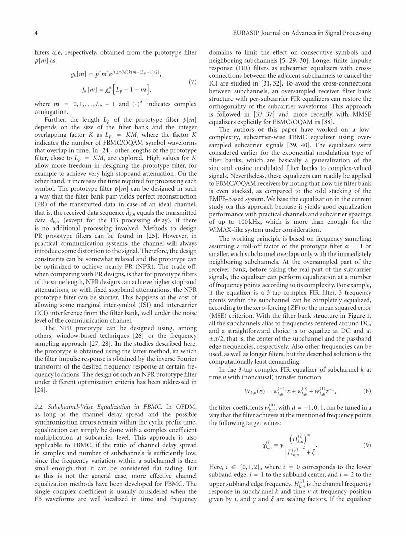
4 EURASIP Journal on Advances in Signal Processing
filters are, respectively, obtained from the prototype filterp[m] as
gk[m] = p[m]e j(2π/M)k(m−(Lp−1)/2),
fk[m] = g∗k[Lp − 1−m
],
(7)
where m = 0, 1, . . . ,Lp − 1 and (·)∗ indicates complexconjugation.
Further, the length Lp of the prototype filter p[m]depends on the size of the filter bank and the integeroverlapping factor K as Lp = KM, where the factor Kindicates the number of FBMC/OQAM symbol waveformsthat overlap in time. In [24], other lengths of the prototypefilter, close to Lp = KM, are explored. High values for Kallow more freedom in designing the prototype filter, forexample to achieve very high stopband attenuation. On theother hand, it increases the time required for processing eachsymbol. The prototype filter p[m] can be designed in sucha way that the filter bank pair yields perfect reconstruction(PR) of the transmitted data in case of an ideal channel,that is, the received data sequence dk,n equals the transmitteddata dk,n (except for the FB processing delay), if thereis no additional processing involved. Methods to designPR prototype filters can be found in [25]. However, inpractical communication systems, the channel will alwaysintroduce some distortion to the signal. Therefore, the designconstraints can be somewhat relaxed and the prototype canbe optimized to achieve nearly PR (NPR). The trade-off,when comparing with PR designs, is that for prototype filtersof the same length, NPR designs can achieve higher stopbandattenuations, or with fixed stopband attenuations, the NPRprototype filter can be shorter. This happens at the cost ofallowing some marginal intersymbol (ISI) and intercarrier(ICI) interference from the filter bank, well under the noiselevel of the communication channel.
The NPR prototype can be designed using, amongothers, window-based techniques [26] or the frequencysampling approach [27, 28]. In the studies described here,the prototype is obtained using the latter method, in whichthe filter impulse response is obtained by the inverse Fouriertransform of the desired frequency response at certain fre-quency locations. The design of such an NPR prototype filterunder different optimization criteria has been addressed in[24].
2.2. Subchannel-Wise Equalization in FBMC. In OFDM,as long as the channel delay spread and the possiblesynchronization errors remain within the cyclic prefix time,equalization can simply be done with a complex coefficientmultiplication at subcarrier level. This approach is alsoapplicable to FBMC, if the ratio of channel delay spreadin samples and number of subchannels is sufficiently low,since the frequency variation within a subchannel is thensmall enough that it can be considered flat fading. Butas this is not the general case, more effective channelequalization methods have been developed for FBMC. Thesingle complex coefficient is usually considered when theFB waveforms are well localized in time and frequency
domains to limit the effect on consecutive symbols andneighboring subchannels [5, 29, 30]. Longer finite impulseresponse (FIR) filters as subcarrier equalizers with cross-connections between the adjacent subchannels to cancel theICI are studied in [31, 32]. To avoid the cross-connectionsbetween subchannels, an oversampled receiver filter bankstructure with per-subcarrier FIR equalizers can restore theorthogonality of the subcarrier waveforms. This approachis followed in [33–37] and more recently with MMSEequalizers explicitly for FBMC/OQAM in [38].
The authors of this paper have worked on a low-complexity, subcarrier-wise FBMC equalizer using over-sampled subcarrier signals [39, 40]. The equalizers wereconsidered earlier for the exponential modulation type offilter banks, which are basically a generalization of thesine and cosine modulated filter banks to complex-valuedsignals. Nevertheless, these equalizers can readily be appliedto FBMC/OQAM receivers by noting that now the filter bankis even stacked, as compared to the odd stacking of theEMFB-based system. We base the equalization in the currentstudy on this approach because it yields good equalizationperformance with practical channels and subcarrier spacingsof up to 100 kHz, which is more than enough for theWiMAX-like system under consideration.
The working principle is based on frequency sampling:assuming a roll-off factor of the prototype filter α = 1 orsmaller, each subchannel overlaps only with the immediatelyneighboring subchannels. At the oversampled part of thereceiver bank, before taking the real part of the subcarriersignals, the equalizer can perform equalization at a numberof frequency points according to its complexity. For example,if the equalizer is a 3-tap complex FIR filter, 3 frequencypoints within the subchannel can be completely equalized,according to the zero-forcing (ZF) or the mean squared error(MSE) criterion. With the filter bank structure in Figure 1,all the subchannels alias to frequencies centered around DC,and a straightforward choice is to equalize at DC and at±π/2, that is, the center of the subchannel and the passbandedge frequencies, respectively. Also other frequencies can beused, as well as longer filters, but the described solution is thecomputationally least demanding.
In the 3-tap complex FIR equalizer of subchannel k attime n with (noncausal) transfer function
Wk,n(z) = w(−1)k,n z +w(0)
k,n +w(1)k,nz
−1, (8)
the filter coefficientsw(d)k,n , with d = −1, 0, 1, can be tuned in a
way that the filter achieves at the mentioned frequency pointsthe following target values:
χ(i)k,n = γ
(H(i)k,n
)∗
∣∣∣H(i)k,n
∣∣∣2
+ ξ. (9)
Here, i ∈ {0, 1, 2}, where i = 0 corresponds to the lowersubband edge, i = 1 to the subband center, and i = 2 to the
upper subband edge frequency. H(i)k,n is the channel frequency
response in subchannel k and time n at frequency positiongiven by i, and γ and ξ are scaling factors. If the equalizer
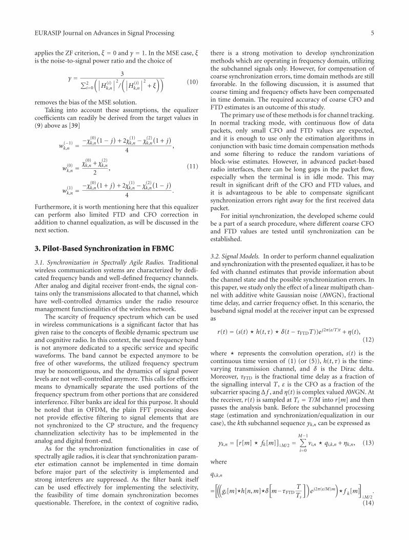
EURASIP Journal on Advances in Signal Processing 5
applies the ZF criterion, ξ = 0 and γ = 1. In the MSE case, ξis the noise-to-signal power ratio and the choice of
γ = 3∑2
i=0
(∣∣∣H(i)k,n
∣∣∣2/(∣∣∣H(i)
k,n
∣∣∣2
+ ξ))
(10)
removes the bias of the MSE solution.Taking into account these assumptions, the equalizer
coefficients can readily be derived from the target values in(9) above as [39]
w(−1)k,n = −χ(0)
k,n
(1− j
)+ 2χ(1)
k,n − χ(2)k,n
(1 + j
)
4,
w(0)k,n =
χ(0)k,n + χ(2)
k,n
2,
w(1)k,n =
−χ(0)k,n
(1 + j
)+ 2χ(1)
k,n − χ(2)k,n
(1− j
)
4.
(11)
Furthermore, it is worth mentioning here that this equalizercan perform also limited FTD and CFO correction inaddition to channel equalization, as will be discussed in thenext section.
3. Pilot-Based Synchronization in FBMC
3.1. Synchronization in Spectrally Agile Radios. Traditionalwireless communication systems are characterized by dedi-cated frequency bands and well-defined frequency channels.After analog and digital receiver front-ends, the signal con-tains only the transmissions allocated to that channel, whichhave well-controlled dynamics under the radio resourcemanagement functionalities of the wireless network.
The scarcity of frequency spectrum which can be usedin wireless communications is a significant factor that hasgiven raise to the concepts of flexible dynamic spectrum useand cognitive radio. In this context, the used frequency bandis not anymore dedicated to a specific service and specificwaveforms. The band cannot be expected anymore to befree of other waveforms, the utilized frequency spectrummay be noncontiguous, and the dynamics of signal powerlevels are not well-controlled anymore. This calls for efficientmeans to dynamically separate the used portions of thefrequency spectrum from other portions that are consideredinterference. Filter banks are ideal for this purpose. It shouldbe noted that in OFDM, the plain FFT processing doesnot provide effective filtering to signal elements that arenot synchronized to the CP structure, and the frequencychannelization selectivity has to be implemented in theanalog and digital front-end.
As for the synchronization functionalities in case ofspectrally agile radios, it is clear that synchronization param-eter estimation cannot be implemented in time domainbefore major part of the selectivity is implemented andstrong interferers are suppressed. As the filter bank itselfcan be used effectively for implementing the selectivity,the feasibility of time domain synchronization becomesquestionable. Therefore, in the context of cognitive radio,
there is a strong motivation to develop synchronizationmethods which are operating in frequency domain, utilizingthe subchannel signals only. However, for compensation ofcoarse synchronization errors, time domain methods are stillfavorable. In the following discussion, it is assumed thatcoarse timing and frequency offsets have been compensatedin time domain. The required accuracy of coarse CFO andFTD estimates is an outcome of this study.
The primary use of these methods is for channel tracking.In normal tracking mode, with continuous flow of datapackets, only small CFO and FTD values are expected,and it is enough to use only the estimation algorithms inconjunction with basic time domain compensation methodsand some filtering to reduce the random variations ofblock-wise estimates. However, in advanced packet-basedradio interfaces, there can be long gaps in the packet flow,especially when the terminal is in idle mode. This mayresult in significant drift of the CFO and FTD values, andit is advantageous to be able to compensate significantsynchronization errors right away for the first received datapacket.
For initial synchronization, the developed scheme couldbe a part of a search procedure, where different coarse CFOand FTD values are tested until synchronization can beestablished.
3.2. Signal Models. In order to perform channel equalizationand synchronization with the presented equalizer, it has to befed with channel estimates that provide information aboutthe channel state and the possible synchronization errors. Inthis paper, we study only the effect of a linear multipath chan-nel with additive white Gaussian noise (AWGN), fractionaltime delay, and carrier frequency offset. In this scenario, thebaseband signal model at the receiver input can be expressedas
r(t) = (s(t)� h(t, τ)� δ(t − τFTDT))e j2π(ε/T)t + η(t),(12)
where � represents the convolution operation, s(t) is thecontinuous time version of (1) (or (5)), h(t, τ) is the time-varying transmission channel, and δ is the Dirac delta.Moreover, τFTD is the fractional time delay as a fraction ofthe signalling interval T , ε is the CFO as a fraction of thesubcarrier spacingΔ f , and η(t) is complex valued AWGN. Atthe receiver, r(t) is sampled at Ts = T/M into r[m] and thenpasses the analysis bank. Before the subchannel processingstage (estimation and synchronization/equalization in ourcase), the kth subchannel sequence yk,n can be expressed as
yk,n =[r[m]� fk[m]
]↓M/2 =
M−1∑
i=0
vi,n � qi,k,n + ηk,n, (13)
where
qi,k,n
=[((gi[m]�h[n,m]�δ
[m−τFTD
T
Ts
])e j2π(ε/M)m
)�f k[m]
]
↓M/2.
(14)
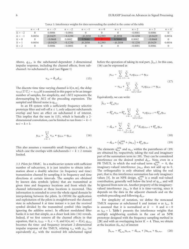
6 EURASIP Journal on Advances in Signal Processing
Table 1: Interference weights for data surrounding the symbol in the center of the table
n = −4 n = −3 n = −2 n = −1 n = 0 n = 1 n = 2 n = 3 n = 4k = −2 0 0.0006 −0.0001 0 0 0 −0.0001 0.0006 0k = −1 0.0054 j0.0429 −0.1250 −j0.2058 0.2393 j0.2058 −0.1250 −j0.0429 0.0054k = 0 0 −0.0668 0.0002 0.5644 1 0.5644 0.0002 −0.0668 0k = 1 0.0054 −j0.0429 −0.1250 j0.2058 0.2393 −j0.2058 −0.1250 j0.0429 0.0054k = 2 0 0.0006 −0.0001 0 0 0 −0.0001 0.0006 0
Above, qi,k,n is the subchannel-dependent 2-dimensionalimpulse response, including the channel effects, from sub-channel i to subchannel k, and (see Figure 1)
vi,n = θi,ndi,n. (15)
The discrete-time time varying channel is h[n,m], the delayτFTD(T/Ts) = τFTDM is assumed in this paper to be an integernumber of samples, for simplicity, and ↓M/2 represents thedownsampling by M/2 of the preceding expression. Thesampled and filtered noise is ηk,n.
In an FB system with a sufficiently frequency selectiveprototype filter and roll-off α ≤ 1, only adjacent subchannelsoverlap and have an effect on subchannel k of interest.This implies that the sum in (13), which is basically a 2-dimensional convolution, can be limited to run from i = k−1to i = k + 1:
yk,n =k+1∑
i=k−1
vi,n � qi,k,n + ηk,n. (16)
This also assumes a reasonably small frequency offset ε, inwhich case the overlaps with subchannels i = k ± 2 remainlimited.
3.3. Pilots for FBMC. In a multicarrier system with sufficientnumber of subcarriers, it is just intuitive to obtain infor-mation about a doubly selective (in frequency and time)transmission channel by sampling it in frequency and timedirections at certain intervals. The samples are obtainedby known data symbols (pilots) that are transmitted atgiven time and frequency locations and from which thechannel information at these locations is recovered. Thisinformation is extended to cover the whole signal domain byinterpolating between the pilots. In OFDM the applicationand exploitation of the pilots is straightforward: the channelstate in subchannel k at time instant n is just the receivedsymbol divided by the transmitted symbol (this impliesignoring the additive noise). In efficient modulated filterbanks it is not that simple, as a closer look into (14) reveals.Indeed, if we first remove all the channel effects in thatequation, that is, τFTD = 0, ε = 0, and h[n,m] = δ[n], qi,k,n
becomes the time- and frequency invariant 2-dimensionalimpulse response of the TMUX, relating vi,n with yk,n (orequivalently di,n with the received kth subchannel signal
before the operation of taking its real part, yk,n). In this case,(16) can be expressed as
yk,n =k+1∑
i=k−1
∞∑
l=−∞vi,lqi,k,n−l + ηk,n
= vk,n +k+1∑
i=k−1
∞∑
l=−∞(i,l) /= (k,n)
vi,lqi,k,n−l + ηk,n.
(17)
Equivalently, we can write
yk,n = θ∗k,nyk,n
= θ∗k,nvk,n + θ∗k,n
k+1∑
i=k−1
∞∑
l=−∞(i,l) /= (k,n)
vi,lqi,k,n−l + θ∗k,nηk,n
= dk,n +k+1∑
i=k−1
∞∑
l=−∞(i,l) /= (k,n)
ji−kdi,lqi,k,n−l + θ∗k,nηk,n
(18)
= dk,n +(ηNPRk,n + juk,n
)+ θ∗k,nηk,n. (19)
The elements ηNPRk,n and uk,n within the parentheses of (19)
are obtained by, respectively, taking the real and imaginarypart of the summation term in (18). They can be consideredinterference on the desired symbol dk,n. Now, even in aPR TMUX, in which the real-valued term ηNPR
k,n = 0, theimaginary-valued interference juk,n does not add up to 0.The orthogonality is only obtained after taking the realpart, that is, this interference summation has only imaginaryvalues [5]. In an NPR design, ηNPR
k,n is a small real-valuedcontribution, generally well below the level of ηk,n, and willbe ignored from now on. Another property of the imaginary-valued interference juk,n is that it is time-varying, since itdepends on the data in the adjacent channels and on thesymbols preceding and following dk,n.
For simplicity of notation, we define the noncausalTMUX response at subchannel k and instant n as tk,n. Itis assumed that it is normalized at k = 0 and n = 0as t0,0 = 1. Table 1 presents the interference weights thatmultiply neighboring symbols in the case of an NPRprototype designed with the frequency sampling method in[28] and with an overlapping factor K = 4. Thus, we obtainat the location (k0,n0) of interest
yk0,n0 = θ∗k0,n0yk0,n0 = dk0,n0 + juk0,n0 + ηk0,n0 , (20)
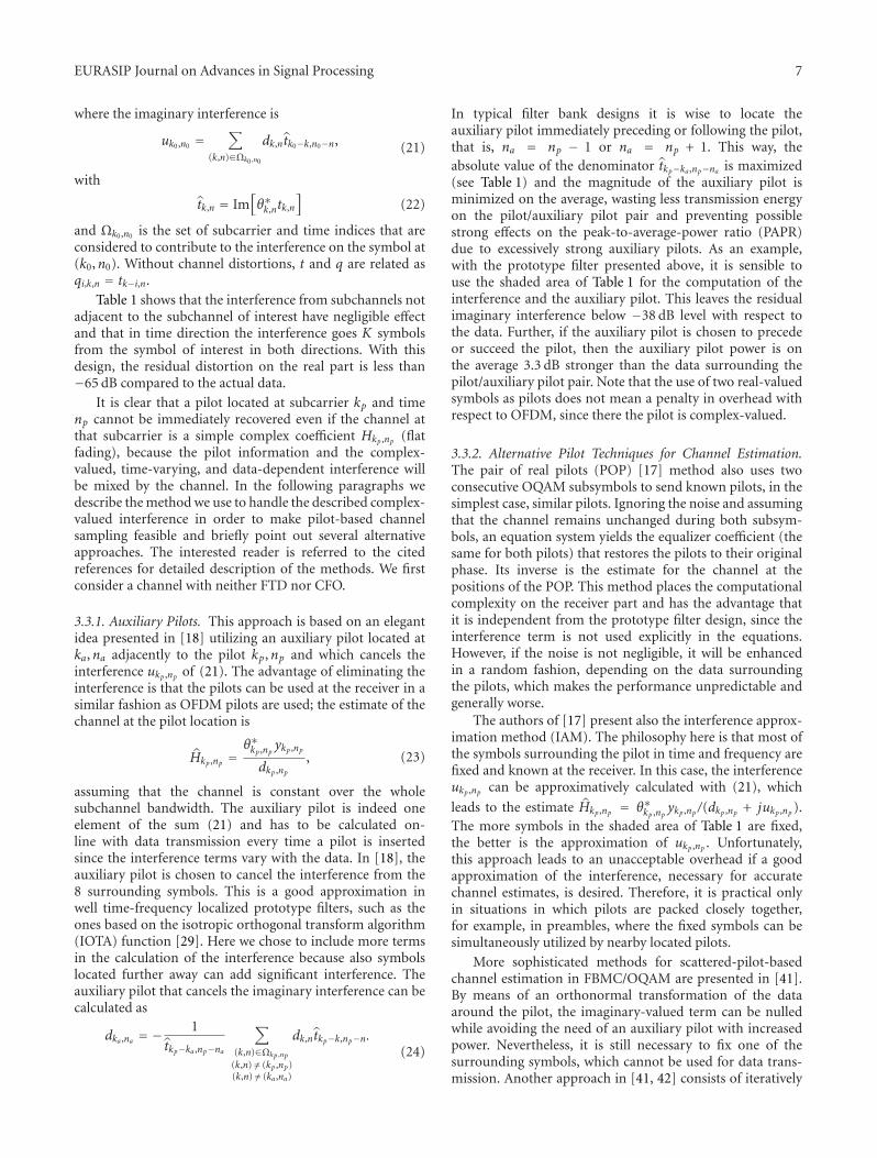
EURASIP Journal on Advances in Signal Processing 7
where the imaginary interference is
uk0,n0 =∑
(k,n)∈Ωk0,n0
dk,ntk0−k,n0−n, (21)
with
tk,n = Im[θ∗k,ntk,n
](22)
and Ωk0,n0 is the set of subcarrier and time indices that areconsidered to contribute to the interference on the symbol at(k0,n0). Without channel distortions, t and q are related asqi,k,n = tk−i,n.
Table 1 shows that the interference from subchannels notadjacent to the subchannel of interest have negligible effectand that in time direction the interference goes K symbolsfrom the symbol of interest in both directions. With thisdesign, the residual distortion on the real part is less than−65 dB compared to the actual data.
It is clear that a pilot located at subcarrier kp and timenp cannot be immediately recovered even if the channel atthat subcarrier is a simple complex coefficient Hkp ,np (flatfading), because the pilot information and the complex-valued, time-varying, and data-dependent interference willbe mixed by the channel. In the following paragraphs wedescribe the method we use to handle the described complex-valued interference in order to make pilot-based channelsampling feasible and briefly point out several alternativeapproaches. The interested reader is referred to the citedreferences for detailed description of the methods. We firstconsider a channel with neither FTD nor CFO.
3.3.1. Auxiliary Pilots. This approach is based on an elegantidea presented in [18] utilizing an auxiliary pilot located atka,na adjacently to the pilot kp,np and which cancels theinterference ukp ,np of (21). The advantage of eliminating theinterference is that the pilots can be used at the receiver in asimilar fashion as OFDM pilots are used; the estimate of thechannel at the pilot location is
Hkp ,np =θ∗kp ,np ykp ,np
dkp ,np, (23)
assuming that the channel is constant over the wholesubchannel bandwidth. The auxiliary pilot is indeed oneelement of the sum (21) and has to be calculated on-line with data transmission every time a pilot is insertedsince the interference terms vary with the data. In [18], theauxiliary pilot is chosen to cancel the interference from the8 surrounding symbols. This is a good approximation inwell time-frequency localized prototype filters, such as theones based on the isotropic orthogonal transform algorithm(IOTA) function [29]. Here we chose to include more termsin the calculation of the interference because also symbolslocated further away can add significant interference. Theauxiliary pilot that cancels the imaginary interference can becalculated as
dka ,na = −1
tkp−ka ,np−na
∑
(k,n)∈Ωkp ,np
(k,n) /= (kp ,np)(k,n) /= (ka,na)
dk,ntkp−k,np−n.(24)
In typical filter bank designs it is wise to locate theauxiliary pilot immediately preceding or following the pilot,that is, na = np − 1 or na = np + 1. This way, theabsolute value of the denominator tkp−ka ,np−na is maximized(see Table 1) and the magnitude of the auxiliary pilot isminimized on the average, wasting less transmission energyon the pilot/auxiliary pilot pair and preventing possiblestrong effects on the peak-to-average-power ratio (PAPR)due to excessively strong auxiliary pilots. As an example,with the prototype filter presented above, it is sensible touse the shaded area of Table 1 for the computation of theinterference and the auxiliary pilot. This leaves the residualimaginary interference below −38 dB level with respect tothe data. Further, if the auxiliary pilot is chosen to precedeor succeed the pilot, then the auxiliary pilot power is onthe average 3.3 dB stronger than the data surrounding thepilot/auxiliary pilot pair. Note that the use of two real-valuedsymbols as pilots does not mean a penalty in overhead withrespect to OFDM, since there the pilot is complex-valued.
3.3.2. Alternative Pilot Techniques for Channel Estimation.The pair of real pilots (POP) [17] method also uses twoconsecutive OQAM subsymbols to send known pilots, in thesimplest case, similar pilots. Ignoring the noise and assumingthat the channel remains unchanged during both subsym-bols, an equation system yields the equalizer coefficient (thesame for both pilots) that restores the pilots to their originalphase. Its inverse is the estimate for the channel at thepositions of the POP. This method places the computationalcomplexity on the receiver part and has the advantage thatit is independent from the prototype filter design, since theinterference term is not used explicitly in the equations.However, if the noise is not negligible, it will be enhancedin a random fashion, depending on the data surroundingthe pilots, which makes the performance unpredictable andgenerally worse.
The authors of [17] present also the interference approx-imation method (IAM). The philosophy here is that most ofthe symbols surrounding the pilot in time and frequency arefixed and known at the receiver. In this case, the interferenceukp ,np can be approximatively calculated with (21), which
leads to the estimate Hkp ,np = θ∗kp ,np ykp ,np /(dkp ,np + jukp ,np).The more symbols in the shaded area of Table 1 are fixed,the better is the approximation of ukp ,np . Unfortunately,this approach leads to an unacceptable overhead if a goodapproximation of the interference, necessary for accuratechannel estimates, is desired. Therefore, it is practical onlyin situations in which pilots are packed closely together,for example, in preambles, where the fixed symbols can besimultaneously utilized by nearby located pilots.
More sophisticated methods for scattered-pilot-basedchannel estimation in FBMC/OQAM are presented in [41].By means of an orthonormal transformation of the dataaround the pilot, the imaginary-valued term can be nulledwhile avoiding the need of an auxiliary pilot with increasedpower. Nevertheless, it is still necessary to fix one of thesurrounding symbols, which cannot be used for data trans-mission. Another approach in [41, 42] consists of iteratively
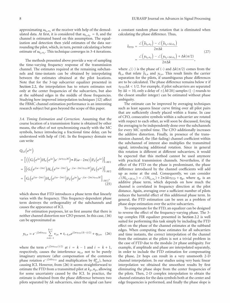
8 EURASIP Journal on Advances in Signal Processing
approximating ukp ,np at the receiver with help of the demod-ulated data. At first, it is considered that ukp ,np = 0, and thechannel is estimated based on this assumption. The equal-ization and detection then yield estimates of the data sur-rounding the pilot, which, in turn, permit calculating a betterestimate of ukp ,np . This technique converges in 3-4 iterations.
The methods presented above provide a way of samplingthe time-varying frequency response of the transmissionchannel. The estimates required at the remaining subchan-nels and time-instants can be obtained by interpolatingbetween the estimates obtained at the pilot locations.Note that for the 3-tap subcarrier equalizer presented inSection 2.2, the interpolation has to return estimates notonly at the center frequencies of the subcarriers, but alsoat the subband edges in the middle of those frequencies.Studying how improved interpolation techniques [12] affectthe FBMC channel estimation performance is an interestingresearch subject but goes beyond the scope of this paper.
3.4. Timing Estimation and Correction. Assuming that thecoarse location of a transmission frame is obtained by othermeans, the effect of not synchronizing exactly with the MCsymbols, hence introducing a fractional time delay, can beunderstood with help of (14). In the frequency domain wecan write
Qi,k
(e jω)
=[((
Gi
(e jω)Hn
(e jω)e− jωτFTDM
)�δ(ω−2πε)
)Fk(e jω)]↓M/2
=[(Gi
(e j(ω−2πε)
)Hn
(e j(ω−2πε)
)e− j(ω−2πε)τFTDM
)Fk(e jω)]↓M/2
=[Gi
(e j(ω−2πε)
)Hn
(e j(ω−2πε)
)Fk(e jω)e− j(ω−2πε)τFTDM
]↓M/2,
(25)
which shows that FTD introduces a phase term that linearlyvaries with the frequency. This frequency-dependent phaseterm destroys the orthogonality of the subchannels andcauses the appearance of ICI.
For estimation purposes, let us first assume that there isneither channel distortion nor CFO present. In this case, (16)can be approximated as
yk,n � e− j2πkτFTD
k+1∑
i=k−1
vi,n � ti−k,nej2πτFTD((k−i)/2) + ηk,n, (26)
where the term e± j2πτFTD(1/2) at i = k − 1 and i = k + 1,respectively, causes the interference uk,n not to be purelyimaginary anymore (after compensation of the commonphase rotation e− j2πkτFTD and multiplication by θ∗k,n), hencecausing ICI. However, from (26) it seems straightforward toestimate the FTD from a transmitted pilot at kp,np, allowingfor some uncertainty caused by the ICI. In practice, theestimate is obtained from the phase difference between twopilots separated by Δk subcarriers, since the signal can have
a constant random phase rotation that is eliminated whencalculating the phase difference. Thus,
τFTD =∠(ykp ,np
)−∠
(ykp+Δk,np
)
2πΔk
=∠(ykp ,np
)−∠
(ykp+Δk,np
)+ Δk(π/2)
2πΔk,
(27)
where ∠(·) is the phase of (·) and Δk(π/2) comes from theθk,n that relate yk,n and yk,n. This result limits the carrierseparation for the pilots, if unambiguous phase differencesare to be calculated. The phase difference remains below π ifτFTDΔk < 1/2. For example, if pilot subcarriers are separatedby Δk = 10, only a delay of ±�M/20 samples (�· rounds tothe closest smaller integer) can be estimated without phaseambiguity.
The estimate can be improved by averaging techniquessuch as least squares linear curve fitting over all pilot pairsthat are sufficiently closely placed within a frame. In caseof CFO, consecutive symbols within a subcarrier are rotatedwith respect to each other, as will soon be discussed, forcingthe averaging to be independently done over the subchannelsfor every MC symbol time. The CFO additionally increasesthe additive distortion. Finally, in presence of the trans-mission channel, the (flat-fading) channel coefficient withinthe subchannel of interest also multiplies the transmittedsignal, introducing additional rotation. Since in generalthis rotation is different at different subcarriers, it wouldbe expected that this method cannot be used anymorewith practical transmission channels. Nevertheless, if theeffect of the FTD on the phase is predominant, the phasedifference introduced by the channel coefficients will addup as noise at the end. Consequently, we can consider∠(Hkp+Δk,np) = ∠(Hkp ,np) + 2πΔkτFTD + ηϕ, where ηϕ is anadditive phase term, which depends on how much thechannel is correlated in frequency direction at the pilotdistance. Again, averaging over a sufficient number of pilotsreduces the harmful effect of this additional phase term. Ingeneral, the FTD estimation can be seen as a problem ofphase slope estimation over the active subcarriers.
To compensate for the FTD, an equalizer can be designedto reverse the effect of the frequency-varying phase. The 3-tap complex FIR equalizer presented in Section 2.2 is wellsuited for performing this task simply by including the FTDeffect on the phase of the channel estimates at the subbandedges. When computing these estimates for all subcarriersand time instants, the correct interpolation of the channelfrom the estimates at the pilots is not a trivial problem inthe case of FTD due to the modulo 2π phase ambiguity. Forexample, if amplitude and phase are interpolated separately,in order to include the FTD estimation for compensatingthe phase, 2π hops can result in a very unsmooth 2-Dchannel interpolation. In our studies using very basic linearinterpolation we obtained the smoothest results by firsteliminating the phase slope from the center frequencies ofthe pilots. Then, 2-D complex interpolation to obtain thechannel estimates for the data symbols both at the center andedge frequencies is performed, and finally the phase slope is
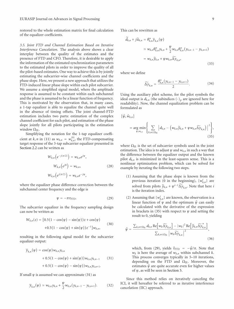
EURASIP Journal on Advances in Signal Processing 9
restored to the whole estimation matrix for final calculationof the equalizer coefficients.
3.5. Joint FTD and Channel Estimation Based on IterativeInterference Cancelation. The analysis above shows a clearinterplay between the quality of the estimates and thepresence of FTD and CFO. Therefore, it is desirable to applythe information of the estimated synchronization parametersto the estimated pilots in order to improve the quality of allthe pilot-based estimates. One way to achieve this is by jointlyestimating the subcarrier-wise channel coefficients and thephase slope. Here, we present a new approach that utilizes theFTD-induced linear phase slope within each pilot subcarrier.We assume a simplified signal model, where the amplituderesponse is assumed to be constant within each subchanneland the phase is assumed to be a linear function of frequency.This is motivated by the observation that, in many cases,a 1-tap equalizer is able to equalize the channel quite wellin the absence of timing offsets. The joint channel-FTDestimation includes two parts: estimation of the complexchannel coefficient for each pilot, and estimation of the phaseslope jointly for all pilots participating in the estimationwindow ΩJE.
Simplifying the notation for the 1-tap equalizer coeffi-
cient at k,n in (11) as wk,n = w(0)k,n, the FTD-compensating
target response of the 3-tap subcarrier equalizer presented inSection 2.2 can be written as
Wk,n
(e− j(π/2)
)= wk,ne
jψ ,
Wk,n
(e j0)= wk,n,
Wk,n
(e j(π/2)
)= wk,ne
− jψ ,
(28)
where the equalizer phase difference correction between thesubchannel center frequency and the edge is
ψ = −πτFTD. (29)
The subcarrier equalizer in the frequency sampling designcan now be written as
Wk,n(z) = [0.5(1− cos(ψ)− sin
(ψ))z + cos
(ψ)
+0.5(1− cos
(ψ)
+ sin(ψ))z−1]wk,n,
(30)
resulting in the following signal model for the subcarrierequalizer output:
yk,n
(ψ) = cos
(ψ)wk,nyk,n
+ 0.5(1− cos
(ψ)
+ sin(ψ))wk,nyk,n−1
+ 0.5(1− cos
(ψ)− sin
(ψ))wk,nyk,n+1.
(31)
If small ψ is assumed we can approximate (31) as
yk,n
(ψ) � wk,nyk,n +
ψ
2wk,n
(yk,n−1 − yk,n+1
). (32)
This can be rewritten as
dk,n + juk,n = θ∗k,nyk,n
(ψ)
� wk,nθ∗k,nyk,n +
ψ
2wk,nθ
∗k,n
(yk,n−1 − yk,n+1
)
= wk,n yk,n + ψwk,nΔyk,n,(33)
where we define
Δyk,n =θ∗k,n
(yk,n−1 − yk,n+1
)
2. (34)
Using the auxiliary pilot scheme, for the pilot symbols theideal output is dk,n (the subindices (·)p are ignored here forreadability). Now, the channel equalization problem can beformulated as
{ψ, wk,n
}
= arg minψ,wk,n
⎧⎨⎩∑
k,n∈ΩJE
∣∣∣dk,n −(wk,n yk,n + ψwk,nΔyk,n
)∣∣∣2
⎫⎬⎭,
(35)
where ΩJE is the set of subcarrier symbols used in the jointestimation. The idea is to adjust ψ andwk,n in such a way thatthe difference between the equalizer output and the knownpilot dk,n is minimized in the least-squares sense. This is anonlinear optimization problem, which can be solved forexample by iterating the following two steps.
(1) Assuming that the phase slope is known from theprevious iteration (0 in the beginning), {wi
k,n} are
solved from pilots yk,n + ψi−1Δyk,n. Note that here iis the iteration index.
(2) Assuming that {wik,n} are known, the observation is a
linear function of ψ and the optimum ψ can easilybe calculated with the derivative of the expressionin brackets in (35) with respect to ψ and setting theresult to 0, yielding
ψ =∑
k,n∈ΩJEdk,n Re
[wkΔyk,n
]− |wk|2 Re
[yk,nΔy
∗k,n
]
∑k,n∈ΩJE
∣∣∣wkΔyk,n
∣∣∣2 ,
(36)
which, from (29), yields τFTD = −ψ/π. Note thatwk is here the average of wk,n within subchannel k.This process converges typically in 5–10 iterations,depending on the FTD and ΩJE. Moreover, theestimates ψ are quite accurate even for higher valuesof ψ, as will be seen in Section 5.
Since this method relies on iteratively canceling theICI, it will hereafter be referred to as iterative interferencecancelation (IIC) approach.
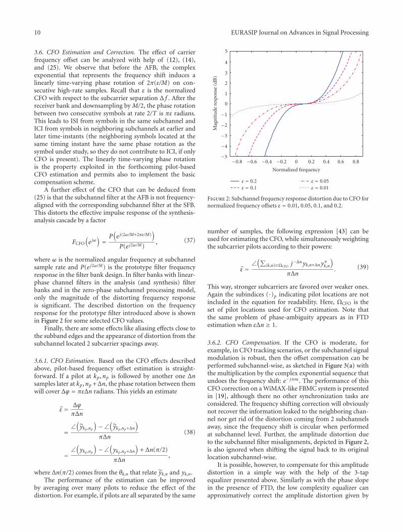
10 EURASIP Journal on Advances in Signal Processing
3.6. CFO Estimation and Correction. The effect of carrierfrequency offset can be analyzed with help of (12), (14),and (25). We observe that before the AFB, the complexexponential that represents the frequency shift induces alinearly time-varying phase rotation of 2π(ε/M) on con-secutive high-rate samples. Recall that ε is the normalizedCFO with respect to the subcarrier separation Δ f . After thereceiver bank and downsampling by M/2, the phase rotationbetween two consecutive symbols at rate 2/T is πε radians.This leads to ISI from symbols in the same subchannel andICI from symbols in neighboring subchannels at earlier andlater time-instants (the neighboring symbols located at thesame timing instant have the same phase rotation as thesymbol under study, so they do not contribute to ICI, if onlyCFO is present). The linearly time-varying phase rotationis the property exploited in the forthcoming pilot-basedCFO estimation and permits also to implement the basiccompensation scheme.
A further effect of the CFO that can be deduced from(25) is that the subchannel filter at the AFB is not frequency-aligned with the corresponding subchannel filter at the SFB.This distorts the effective impulse response of the synthesis-analysis cascade by a factor
FCFO
(e jω)=P(e j(2ω/M+2πε/M)
)
P(e j2ω/M), (37)
where ω is the normalized angular frequency at subchannelsample rate and P(e j2ω/M) is the prototype filter frequencyresponse in the filter bank design. In filter banks with linear-phase channel filters in the analysis (and synthesis) filterbanks and in the zero-phase subchannel processing model,only the magnitude of the distorting frequency responseis significant. The described distortion on the frequencyresponse for the prototype filter introduced above is shownin Figure 2 for some selected CFO values.
Finally, there are some effects like aliasing effects close tothe subband edges and the appearance of distortion from thesubchannel located 2 subcarrier spacings away.
3.6.1. CFO Estimation. Based on the CFO effects describedabove, pilot-based frequency offset estimation is straight-forward. If a pilot at kp,np is followed by another one Δnsamples later at kp,np +Δn, the phase rotation between themwill cover Δϕ = πεΔn radians. This yields an estimate
ε = Δϕ
πΔn
=∠(ykp ,np
)−∠
(ykp ,np+Δn
)
πΔn
=∠(ykp ,np
)−∠
(ykp ,np+Δn
)+ Δn(π/2)
πΔn,
(38)
where Δn(π/2) comes from the θk,n that relate yk,n and yk,n.The performance of the estimation can be improved
by averaging over many pilots to reduce the effect of thedistortion. For example, if pilots are all separated by the same
−5
−4
−3
−2
−1
0
1
2
3
4
5
Mag
nit
ude
resp
onse
(dB
)
−0.8 −0.6 −0.4 −0.2 0 0.2 0.4 0.6 0.8
Normalized frequency
ε = 0.2ε = 0.1
ε = 0.05ε = 0.01
Figure 2: Subchannel frequency response distortion due to CFO fornormalized frequency offsets ε = 0.01, 0.05, 0.1, and 0.2.
number of samples, the following expression [43] can beused for estimating the CFO, while simultaneously weightingthe subcarrier pilots according to their powers:
ε =∠(∑
(k,n)∈ΩCFOj−Δnyk,n+Δny
∗k,n
)
πΔn. (39)
This way, stronger subcarriers are favored over weaker ones.Again the subindices (·)p indicating pilot locations are notincluded in the equation for readability. Here, ΩCFO is theset of pilot locations used for CFO estimation. Note thatthe same problem of phase-ambiguity appears as in FTDestimation when εΔn ≥ 1.
3.6.2. CFO Compensation. If the CFO is moderate, forexample, in CFO tracking scenarios, or the subchannel signalmodulation is robust, then the offset compensation can beperformed subchannel-wise, as sketched in Figure 3(a) withthe multiplication by the complex exponential sequence thatundoes the frequency shift: e− jπnε. The performance of thisCFO correction on a WiMAX-like FBMC system is presentedin [19], although there no other synchronization tasks areconsidered. The frequency shifting correction will obviouslynot recover the information leaked to the neighboring chan-nel nor get rid of the distortion coming from 2 subchannelsaway, since the frequency shift is circular when performedat subchannel level. Further, the amplitude distortion dueto the subchannel filter misalignments, depicted in Figure 2,is also ignored when shifting the signal back to its originallocation subchannel-wise.
It is possible, however, to compensate for this amplitudedistortion in a simple way with the help of the 3-tapequalizer presented above. Similarly as with the phase slopein the presence of FTD, the low complexity equalizer canapproximatively correct the amplitude distortion given by
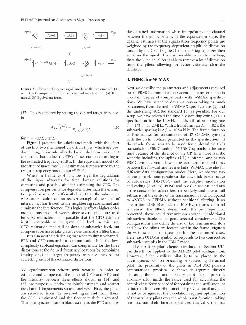
EURASIP Journal on Advances in Signal Processing 11
r[m]
e j2πmε/M
fk[m] M/2
e− jπnε
wk[n]xk,n
(a)
r[m]e− j2πmε/M fk[m] M/2
e jπn(ε−ε)
wk[n]xk,n
(b)
Figure 3: Subchannel receiver signal model in the presence of CFO,with CFO compensation and subchannel equalization. (a) Basicmodel. (b) Equivalent form.
(37). This is achieved by setting the desired target responsesto
Wk,n
(e jω)= 1FCFO(e jω)
, (40)
for ω = −π/2, 0,π/2.Figure 3 presents the subchannel model with the effect
of the first two mentioned distortion types, which are pre-dominating. It includes also the basic subchannel-wise CFOcorrection that undoes the CFO phase rotation according tothe estimated frequency shift ε. In the equivalent model (b),the effect of inaccurate CFO estimation is represented by theresidual frequency modulation e jπn(ε−ε).
When the frequency shift is too large, the degradationof the signal advocates for time domain solutions forcorrecting and possibly also for estimating the CFO. Thecompensation performance degrades faster than the estima-tion performance: At sufficiently high CFO, the subcarrier-wise compensation cannot recover enough of the signal ofinterest that has leaked to the neighboring subchannel andeliminate the interference. This logically affects higher ordermodulations most. However, since several pilots are usedfor CFO estimation, it is possible that the CFO estimateis still acceptable at the given CFO level. In this case,CFO estimation may still be done at subcarrier level, butcompensation has to take place before the analysis filter bank.
It is also worth underlining that when multipath channel,FTD and CFO concur in a communication link, the low-complexity subband equalizer can compensate for the threedistortions at the desired frequency locations by combining(multiplying) the target frequency responses needed forcorrecting each of the estimated distortions.
3.7. Synchronization Scheme with Iteration. In order toestimate and compensate the effect of CFO and FTD andthe interplay between these effects shown in (14) and(25) we propose a receiver to jointly estimate and correctthe channel impairments subchannel-wise. First, the pilotsare recovered from the received signal and from them,the CFO is estimated and the frequency shift is reverted.Then, the synchronization block estimates the FTD and uses
the obtained information when interpolating the channelbetween the pilots. Finally, at the equalization stage, thechannel estimates at the equalization frequency points areweighted by the frequency-dependent amplitude distortioncaused by the CFO (Figure 2) and the 3-tap equalizer thenequalizes the signal. It is also possible to iterate this loop,since the 3-tap equalizer is able to remove a lot of distortionfrom the pilots, allowing for better estimates after theiteration.
4. FBMC for WiMAX
Next we describe the parameters and adjustments requiredfor an FBMC communication system that aims to maintaina certain degree of compatibility with WiMAX specifica-tions. We have aimed to design a system taking as muchparameters from the mobile WiMAX specifications [2] andthe underlying 802.16e standard [3] as possible. For oursetup, we have selected the time division duplexing (TDD)specification for the 10 MHz bandwidth at sampling ratefs = 1/Ts = 11.2 MHz. With a transform size M = 1024, thesubcarrier spacing is Δ f = 10.94 kHz. The frame durationof 5 ms allows for transmission of 47 OFDMA symbolswith the cyclic prefixes permitted in the specifications. Ifthe whole frame was to be used for a downlink (DL)transmission, FBMC could fit 53 FBMC symbols in the sametime because of the absence of the CP. In a more realisticscenario including the uplink (UL) subframe, one or twoFBMC symbols would have to be sacrificed for guard timesbetween the forward and reverse links. WiMAX provides fordifferent data configuration modes. Here, we observe twoof the possible configurations: the downlink partial usageof subcarriers (DL-PUSC) and the adaptive modulationand coding (AMC23). PUSC and AMC23 use 840 and 864active consecutive subcarriers, respectively, and have a nullsubcarrier at the center of the transmission band. Comparedto AMC23 in OFDMA without additional filtering, if anattenuation of 40 dB outside the 10 MHz transmission bandis desired, the FBMC design with the prototype filterpresented above could transmit on around 50 additionalsubcarriers thanks to its good spectral containment. Theconfigurations also define the size of the transmission slotsand how the pilots are located within the frame. Figure 4shows these pilot configurations for the mentioned cases.Here, each OFDMA symbol corresponds to two consecutivesubcarrier samples in the FBMC model.
The auxiliary pilot scheme introduced in Section 3.3.1can directly be applied to the AMC23 pilot configuration.However, if the auxiliary pilot is to be placed in theadvantageous position preceding or succeeding the actualpilot, the proximity of the pilots in DL-PUSC poses acomputational problem. As shown in Figure 5, directlyallocating the pilot and auxiliary pilot fixes a previousauxiliary pilot inside the range used for calculating thecomplex interference needed for obtaining the auxiliary pilotof interest. If the contribution of this previous auxiliary pilotis not to be ignored, the calculation requires optimizationof the auxiliary pilots over the whole burst duration, takinginto account their interdependencies (basically, the first
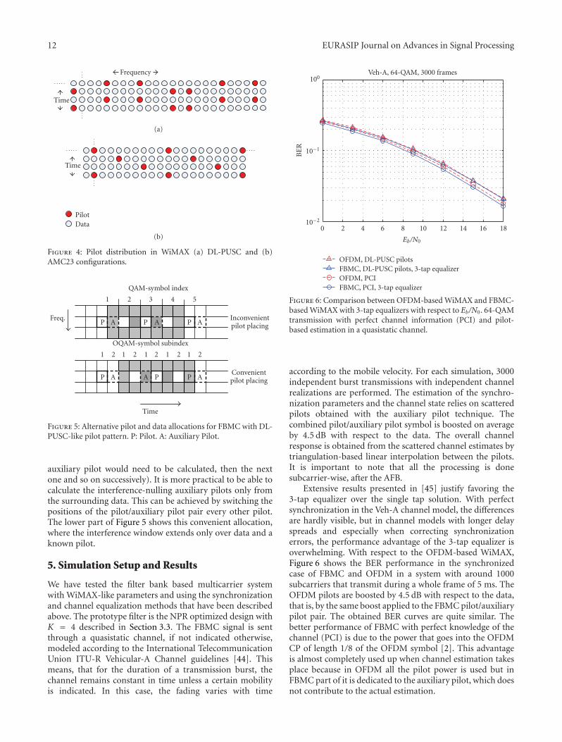
12 EURASIP Journal on Advances in Signal Processing
Frequency
Time
(a)
Time
PilotData
(b)
Figure 4: Pilot distribution in WiMAX (a) DL-PUSC and (b)AMC23 configurations.
Freq.
1 2 3 4 5
QAM-symbol index
P A P A P AInconvenientpilot placing
Convenientpilot placing
OQAM-symbol subindex
1 2 1 2 1 2 1 2 1 2
P A A P P A
Time
Figure 5: Alternative pilot and data allocations for FBMC with DL-PUSC-like pilot pattern. P: Pilot. A: Auxiliary Pilot.
auxiliary pilot would need to be calculated, then the nextone and so on successively). It is more practical to be able tocalculate the interference-nulling auxiliary pilots only fromthe surrounding data. This can be achieved by switching thepositions of the pilot/auxiliary pilot pair every other pilot.The lower part of Figure 5 shows this convenient allocation,where the interference window extends only over data and aknown pilot.
5. Simulation Setup and Results
We have tested the filter bank based multicarrier systemwith WiMAX-like parameters and using the synchronizationand channel equalization methods that have been describedabove. The prototype filter is the NPR optimized design withK = 4 described in Section 3.3. The FBMC signal is sentthrough a quasistatic channel, if not indicated otherwise,modeled according to the International TelecommunicationUnion ITU-R Vehicular-A Channel guidelines [44]. Thismeans, that for the duration of a transmission burst, thechannel remains constant in time unless a certain mobilityis indicated. In this case, the fading varies with time
10−2
10−1
100Veh-A, 64-QAM, 3000 frames
BE
R
0 2 4 6 8 10 12 14 16 18
Eb/N0
OFDM, DL-PUSC pilotsFBMC, DL-PUSC pilots, 3-tap equalizerOFDM, PCIFBMC, PCI, 3-tap equalizer
Figure 6: Comparison between OFDM-based WiMAX and FBMC-based WiMAX with 3-tap equalizers with respect to Eb/N0. 64-QAMtransmission with perfect channel information (PCI) and pilot-based estimation in a quasistatic channel.
according to the mobile velocity. For each simulation, 3000independent burst transmissions with independent channelrealizations are performed. The estimation of the synchro-nization parameters and the channel state relies on scatteredpilots obtained with the auxiliary pilot technique. Thecombined pilot/auxiliary pilot symbol is boosted on averageby 4.5 dB with respect to the data. The overall channelresponse is obtained from the scattered channel estimates bytriangulation-based linear interpolation between the pilots.It is important to note that all the processing is donesubcarrier-wise, after the AFB.
Extensive results presented in [45] justify favoring the3-tap equalizer over the single tap solution. With perfectsynchronization in the Veh-A channel model, the differencesare hardly visible, but in channel models with longer delayspreads and especially when correcting synchronizationerrors, the performance advantage of the 3-tap equalizer isoverwhelming. With respect to the OFDM-based WiMAX,Figure 6 shows the BER performance in the synchronizedcase of FBMC and OFDM in a system with around 1000subcarriers that transmit during a whole frame of 5 ms. TheOFDM pilots are boosted by 4.5 dB with respect to the data,that is, by the same boost applied to the FBMC pilot/auxiliarypilot pair. The obtained BER curves are quite similar. Thebetter performance of FBMC with perfect knowledge of thechannel (PCI) is due to the power that goes into the OFDMCP of length 1/8 of the OFDM symbol [2]. This advantageis almost completely used up when channel estimation takesplace because in OFDM all the pilot power is used but inFBMC part of it is dedicated to the auxiliary pilot, which doesnot contribute to the actual estimation.
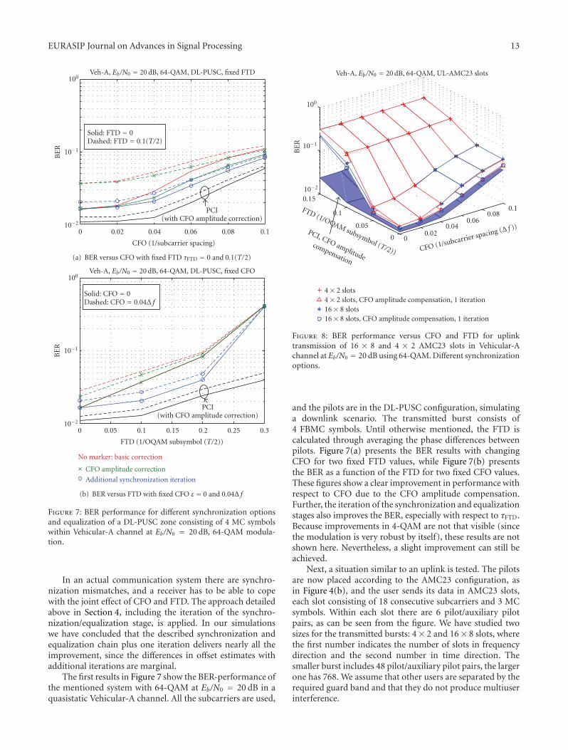
EURASIP Journal on Advances in Signal Processing 13
10−2
10−1
100Veh-A, Eb/N0 = 20 dB, 64-QAM, DL-PUSC, fixed FTD
BE
R
0 0.02 0.04 0.06 0.08 0.1
CFO (1/subcarrier spacing)
Solid: FTD = 0Dashed: FTD = 0.1(T/2)
PCI(with CFO amplitude correction)
(a) BER versus CFO with fixed FTD τFTD = 0 and 0.1(T/2)
10−2
10−1
100Veh-A, Eb/N0 = 20 dB, 64-QAM, DL-PUSC, fixed CFO
BE
R
0 0.05 0.1 0.15 0.2
PCI(with CFO amplitude correction)
0.25 0.3
FTD (1/OQAM subsymbol (T/2))
Solid: CFO = 0Dashed: CFO = 0.04Δ f
No marker: basic correction
CFO amplitude correction
Additional synchronization iteration
(b) BER versus FTD with fixed CFO ε = 0 and 0.04Δ f
Figure 7: BER performance for different synchronization optionsand equalization of a DL-PUSC zone consisting of 4 MC symbolswithin Vehicular-A channel at Eb/N0 = 20 dB, 64-QAM modula-tion.
In an actual communication system there are synchro-nization mismatches, and a receiver has to be able to copewith the joint effect of CFO and FTD. The approach detailedabove in Section 4, including the iteration of the synchro-nization/equalization stage, is applied. In our simulationswe have concluded that the described synchronization andequalization chain plus one iteration delivers nearly all theimprovement, since the differences in offset estimates withadditional iterations are marginal.
The first results in Figure 7 show the BER-performance ofthe mentioned system with 64-QAM at Eb/N0 = 20 dB in aquasistatic Vehicular-A channel. All the subcarriers are used,
10−2
10−1
100
Veh-A, Eb/N0 = 20 dB, 64-QAM, UL-AMC23 slots
0.15
0.1
0.05PCI, CFO amplitude
compensation
0 00.02
0.040.06
0.080.1
BE
R
FTD (1/OQAM subsymbol (T/2)) CFO (1/subcarrier spacing (Δ f ))
4× 2 slots4× 2 slots, CFO amplitude compensation, 1 iteration16× 8 slots16× 8 slots, CFO amplitude compensation, 1 iteration
Figure 8: BER performance versus CFO and FTD for uplinktransmission of 16 × 8 and 4 × 2 AMC23 slots in Vehicular-Achannel at Eb/N0 = 20 dB using 64-QAM. Different synchronizationoptions.
and the pilots are in the DL-PUSC configuration, simulatinga downlink scenario. The transmitted burst consists of4 FBMC symbols. Until otherwise mentioned, the FTD iscalculated through averaging the phase differences betweenpilots. Figure 7(a) presents the BER results with changingCFO for two fixed FTD values, while Figure 7(b) presentsthe BER as a function of the FTD for two fixed CFO values.These figures show a clear improvement in performance withrespect to CFO due to the CFO amplitude compensation.Further, the iteration of the synchronization and equalizationstages also improves the BER, especially with respect to τFTD.Because improvements in 4-QAM are not that visible (sincethe modulation is very robust by itself), these results are notshown here. Nevertheless, a slight improvement can still beachieved.
Next, a situation similar to an uplink is tested. The pilotsare now placed according to the AMC23 configuration, asin Figure 4(b), and the user sends its data in AMC23 slots,each slot consisting of 18 consecutive subcarriers and 3 MCsymbols. Within each slot there are 6 pilot/auxiliary pilotpairs, as can be seen from the figure. We have studied twosizes for the transmitted bursts: 4× 2 and 16× 8 slots, wherethe first number indicates the number of slots in frequencydirection and the second number in time direction. Thesmaller burst includes 48 pilot/auxiliary pilot pairs, the largerone has 768. We assume that other users are separated by therequired guard band and that they do not produce multiuserinterference.
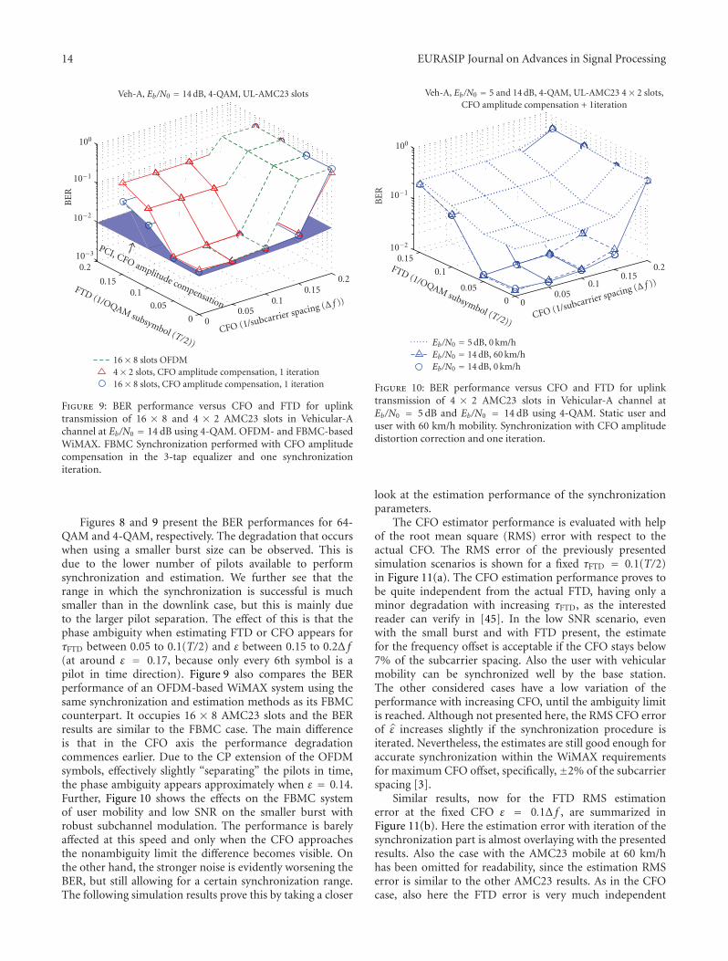
14 EURASIP Journal on Advances in Signal Processing
10−3
10−2
10−1
100
Veh-A, Eb/N0 = 14 dB, 4-QAM, UL-AMC23 slots
0.2
0.150.1
0.05
0 00.05
0.10.15
0.2
BE
R
FTD (1/OQAM subsymbol (T/2))
CFO (1/subcarrier spacing (Δ f ))
16× 8 slots OFDM4× 2 slots, CFO amplitude compensation, 1 iteration16× 8 slots, CFO amplitude compensation, 1 iteration
PCI, CFO amplitude compensation
Figure 9: BER performance versus CFO and FTD for uplinktransmission of 16 × 8 and 4 × 2 AMC23 slots in Vehicular-Achannel at Eb/N0 = 14 dB using 4-QAM. OFDM- and FBMC-basedWiMAX. FBMC Synchronization performed with CFO amplitudecompensation in the 3-tap equalizer and one synchronizationiteration.
Figures 8 and 9 present the BER performances for 64-QAM and 4-QAM, respectively. The degradation that occurswhen using a smaller burst size can be observed. This isdue to the lower number of pilots available to performsynchronization and estimation. We further see that therange in which the synchronization is successful is muchsmaller than in the downlink case, but this is mainly dueto the larger pilot separation. The effect of this is that thephase ambiguity when estimating FTD or CFO appears forτFTD between 0.05 to 0.1(T/2) and ε between 0.15 to 0.2Δ f(at around ε = 0.17, because only every 6th symbol is apilot in time direction). Figure 9 also compares the BERperformance of an OFDM-based WiMAX system using thesame synchronization and estimation methods as its FBMCcounterpart. It occupies 16 × 8 AMC23 slots and the BERresults are similar to the FBMC case. The main differenceis that in the CFO axis the performance degradationcommences earlier. Due to the CP extension of the OFDMsymbols, effectively slightly “separating” the pilots in time,the phase ambiguity appears approximately when ε = 0.14.Further, Figure 10 shows the effects on the FBMC systemof user mobility and low SNR on the smaller burst withrobust subchannel modulation. The performance is barelyaffected at this speed and only when the CFO approachesthe nonambiguity limit the difference becomes visible. Onthe other hand, the stronger noise is evidently worsening theBER, but still allowing for a certain synchronization range.The following simulation results prove this by taking a closer
10−2
10−1
100
Veh-A, Eb/N0 = 5 and 14 dB, 4-QAM, UL-AMC23 4× 2 slots,CFO amplitude compensation + 1iteration
0.15
0.1
0.05
0 00.05
0.10.15
0.2
BE
R
FTD (1/OQAM subsymbol (T/2))CFO (1/subcarrier spacing (Δ f ))
Eb/N0 = 5 dB, 0 km/hEb/N0 = 14 dB, 60 km/hEb/N0 = 14 dB, 0 km/h
Figure 10: BER performance versus CFO and FTD for uplinktransmission of 4 × 2 AMC23 slots in Vehicular-A channel atEb/N0 = 5 dB and Eb/N0 = 14 dB using 4-QAM. Static user anduser with 60 km/h mobility. Synchronization with CFO amplitudedistortion correction and one iteration.
look at the estimation performance of the synchronizationparameters.
The CFO estimator performance is evaluated with helpof the root mean square (RMS) error with respect to theactual CFO. The RMS error of the previously presentedsimulation scenarios is shown for a fixed τFTD = 0.1(T/2)in Figure 11(a). The CFO estimation performance proves tobe quite independent from the actual FTD, having only aminor degradation with increasing τFTD, as the interestedreader can verify in [45]. In the low SNR scenario, evenwith the small burst and with FTD present, the estimatefor the frequency offset is acceptable if the CFO stays below7% of the subcarrier spacing. Also the user with vehicularmobility can be synchronized well by the base station.The other considered cases have a low variation of theperformance with increasing CFO, until the ambiguity limitis reached. Although not presented here, the RMS CFO errorof ε increases slightly if the synchronization procedure isiterated. Nevertheless, the estimates are still good enough foraccurate synchronization within the WiMAX requirementsfor maximum CFO offset, specifically, ±2% of the subcarrierspacing [3].
Similar results, now for the FTD RMS estimationerror at the fixed CFO ε = 0.1Δ f , are summarized inFigure 11(b). Here the estimation error with iteration of thesynchronization part is almost overlaying with the presentedresults. Also the case with the AMC23 mobile at 60 km/hhas been omitted for readability, since the estimation RMSerror is similar to the other AMC23 results. As in the CFOcase, also here the FTD error is very much independent
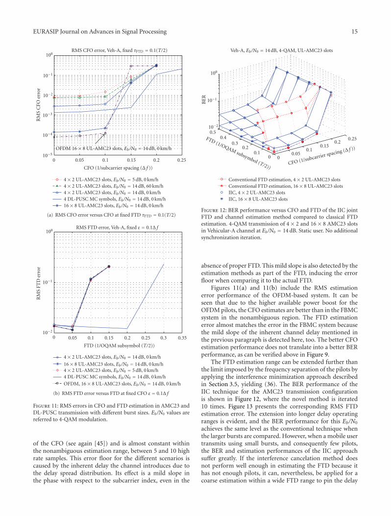
EURASIP Journal on Advances in Signal Processing 15
10−5
10−4
10−3
10−2
10−1
100RMS CFO error, Veh-A, fixed τFTD = 0.1(T/2)
RM
SC
FOer
ror
0 0.05 0.1 0.15 0.2 0.25
CFO (1/subcarrier spacing (Δ f ))
4× 2 UL-AMC23 slots, Eb/N0 = 5 dB, 0 km/h4× 2 UL-AMC23 slots, Eb/N0 = 14 dB, 60 km/h4× 2 UL-AMC23 slots, Eb/N0 = 14 dB, 0 km/h4 DL-PUSC MC symbols, Eb/N0 = 14 dB, 0 km/h16× 8 UL-AMC23 slots, Eb/N0 = 14 dB, 0 km/h
OFDM 16× 8 UL-AMC23 slots, Eb/N0 = 14 dB, 0 km/h
(a) RMS CFO error versus CFO at fixed FTD τFTD = 0.1(T/2)
10−2
10−1
100RMS FTD error, Veh-A, fixed ε = 0.1Δ f
RM
SFT
Der
ror
0 0.05 0.1 0.15 0.2 0.25 0.3 0.35
FTD (1/OQAM subsymbol (T/2))
4× 2 UL-AMC23 slots, Eb/N0 = 14 dB, 0 km/h
16× 8 UL-AMC23 slots, Eb/N0 = 14 dB, 0 km/h4× 2 UL-AMC23 slots, Eb/N0 = 5 dB, 0 km/h4 DL-PUSC MC symbols, Eb/N0 = 14 dB, 0 km/h
OFDM, 16× 8 UL-AMC23 slots, Eb/N0 = 14 dB, 0 km/h
(b) RMS FTD error versus FTD at fixed CFO ε = 0.1Δ f
Figure 11: RMS errors in CFO and FTD estimation in AMC23 andDL-PUSC transmission with different burst sizes. Eb/N0 values arereferred to 4-QAM modulation.
of the CFO (see again [45]) and is almost constant withinthe nonambiguous estimation range, between 5 and 10 highrate samples. This error floor for the different scenarios iscaused by the inherent delay the channel introduces due tothe delay spread distribution. Its effect is a mild slope inthe phase with respect to the subcarrier index, even in the
10−2
10−1
100
Veh-A, Eb/N0 = 14 dB, 4-QAM, UL-AMC23 slots
0.50.4
0.30.2
0.10 0
0.050.1
0.150.2
0.25
BE
R
FTD (1/OQAM subsymbol (T/2))CFO (1/subcarrier spacing (Δ f ))
Conventional FTD estimation, 4× 2 UL-AMC23 slotsConventional FTD estimation, 16× 8 UL-AMC23 slotsIIC, 4× 2 UL-AMC23 slotsIIC, 16× 8 UL-AMC23 slots
Figure 12: BER performance versus CFO and FTD of the IIC jointFTD and channel estimation method compared to classical FTDestimation. 4-QAM transmission of 4 × 2 and 16 × 8 AMC23 slotsin Vehicular-A channel at Eb/N0 = 14 dB. Static user. No additionalsynchronization iteration.
absence of proper FTD. This mild slope is also detected by theestimation methods as part of the FTD, inducing the errorfloor when comparing it to the actual FTD.
Figures 11(a) and 11(b) include the RMS estimationerror performance of the OFDM-based system. It can beseen that due to the higher available power boost for theOFDM pilots, the CFO estimates are better than in the FBMCsystem in the nonambiguous region. The FTD estimationerror almost matches the error in the FBMC system becausethe mild slope of the inherent channel delay mentioned inthe previous paragraph is detected here, too. The better CFOestimation performance does not translate into a better BERperformance, as can be verified above in Figure 9.
The FTD estimation range can be extended further thanthe limit imposed by the frequency separation of the pilots byapplying the interference minimization approach describedin Section 3.5, yielding (36). The BER performance of theIIC technique for the AMC23 transmission configurationis shown in Figure 12, where the novel method is iterated10 times. Figure 13 presents the corresponding RMS FTDestimation error. The extension into longer delay operatingranges is evident, and the BER performance for this Eb/N0
achieves the same level as the conventional technique whenthe larger bursts are compared. However, when a mobile usertransmits using small bursts, and consequently few pilots,the BER and estimation performances of the IIC approachsuffer greatly. If the interference cancelation method doesnot perform well enough in estimating the FTD because ithas not enough pilots, it can, nevertheless, be applied for acoarse estimation within a wide FTD range to pin the delay
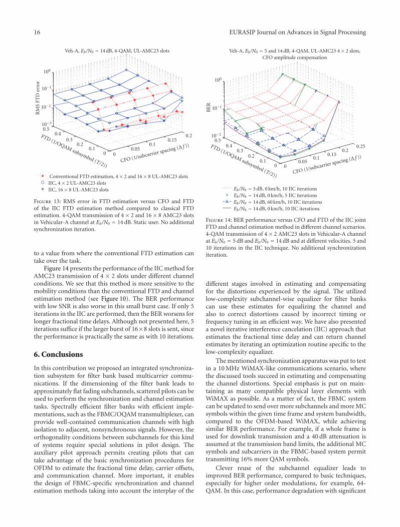
16 EURASIP Journal on Advances in Signal Processing
10−3
10−2
10−1
100
Veh-A, Eb/N0 = 14 dB, 4-QAM, UL-AMC23 slots
0.50.4
0.30.2
0.10 0
0.050.1
0.150.2
RM
SFT
Der
ror
FTD (1/OQAM subsymbol (T/2))CFO (1/subcarrier spacing (Δ f ))
Conventional FTD estimation, 4× 2 and 16× 8 UL-AMC23 slotsIIC, 4× 2 UL-AMC23 slotsIIC, 16× 8 UL-AMC23 slots
Figure 13: RMS error in FTD estimation versus CFO and FTDof the IIC FTD estimation method compared to classical FTDestimation. 4-QAM transmission of 4 × 2 and 16 × 8 AMC23 slotsin Vehicular-A channel at Eb/N0 = 14 dB. Static user. No additionalsynchronization iteration.
to a value from where the conventional FTD estimation cantake over the task.
Figure 14 presents the performance of the IIC method forAMC23 transmission of 4 × 2 slots under different channelconditions. We see that this method is more sensitive to themobility conditions than the conventional FTD and channelestimation method (see Figure 10). The BER performancewith low SNR is also worse in this small burst case. If only 5iterations in the IIC are performed, then the BER worsens forlonger fractional time delays. Although not presented here, 5iterations suffice if the larger burst of 16×8 slots is sent, sincethe performance is practically the same as with 10 iterations.
6. Conclusions
In this contribution we proposed an integrated synchroniza-tion subsystem for filter bank based multicarrier commu-nications. If the dimensioning of the filter bank leads toapproximately flat fading subchannels, scattered pilots can beused to perform the synchronization and channel estimationtasks. Spectrally efficient filter banks with efficient imple-mentations, such as the FBMC/OQAM transmultiplexer, canprovide well-contained communication channels with highisolation to adjacent, nonsynchronous signals. However, theorthogonality conditions between subchannels for this kindof systems require special solutions in pilot design. Theauxiliary pilot approach permits creating pilots that cantake advantage of the basic synchronization procedures forOFDM to estimate the fractional time delay, carrier offsets,and communication channel. More important, it enablesthe design of FBMC-specific synchronization and channelestimation methods taking into account the interplay of the
10−2
10−1
100
Veh-A, Eb/N0 = 5 and 14 dB, 4-QAM, UL-AMC23 4× 2 slots,CFO amplitude compensation
0.50.4
0.30.2
0.10 0
0.050.1
0.150.2
0.25
BE
R
FTD (1/OQAM subsymbol (T/2))CFO (1/subcarrier spacing (Δ f ))
Eb/N0 = 5 dB, 0 km/h, 10 IIC iterationsEb/N0 = 14 dB, 0 km/h, 5 IIC iterationsEb/N0 = 14 dB, 60 km/h, 10 IIC iterationsEb/N0 = 14 dB, 0 km/h, 10 IIC iterations
Figure 14: BER performance versus CFO and FTD of the IIC jointFTD and channel estimation method in different channel scenarios.4-QAM transmission of 4 × 2 AMC23 slots in Vehicular-A channelat Eb/N0 = 5 dB and Eb/N0 = 14 dB and at different velocities. 5 and10 iterations in the IIC technique. No additional synchronizationiteration.
different stages involved in estimating and compensatingfor the distortions experienced by the signal. The utilizedlow-complexity subchannel-wise equalizer for filter bankscan use these estimates for equalizing the channel andalso to correct distortions caused by incorrect timing orfrequency tuning in an efficient way. We have also presenteda novel iterative interference cancelation (IIC) approach thatestimates the fractional time delay and can return channelestimates by iterating an optimization routine specific to thelow-complexity equalizer.
The mentioned synchronization apparatus was put to testin a 10 MHz WiMAX-like communications scenario, wherethe discussed tools succeed in estimating and compensatingthe channel distortions. Special emphasis is put on main-taining as many compatible physical layer elements withWiMAX as possible. As a matter of fact, the FBMC systemcan be updated to send over more subchannels and more MCsymbols within the given time frame and system bandwidth,compared to the OFDM-based WiMAX, while achievingsimilar BER performance. For example, if a whole frame isused for downlink transmission and a 40 dB attenuation isassumed at the transmission band limits, the additional MCsymbols and subcarriers in the FBMC-based system permittransmitting 16% more QAM symbols.
Clever reuse of the subchannel equalizer leads toimproved BER performance, compared to basic techniques,especially for higher order modulations, for example, 64-QAM. In this case, performance degradation with significant
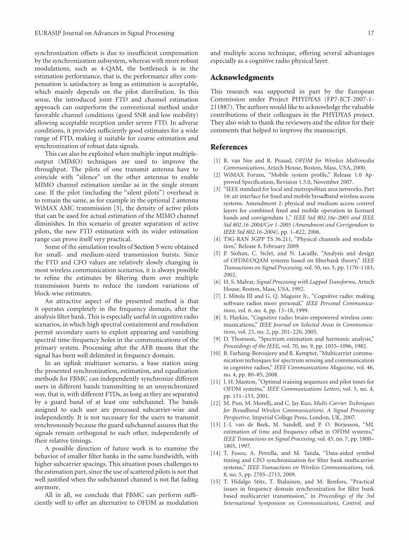
EURASIP Journal on Advances in Signal Processing 17
synchronization offsets is due to insufficient compensationby the synchronization subsystem, whereas with more robustmodulations, such as 4-QAM, the bottleneck is in theestimation performance, that is, the performance after com-pensation is satisfactory as long as estimation is acceptable,which mainly depends on the pilot distribution. In thissense, the introduced joint FTD and channel estimationapproach can outperform the conventional method underfavorable channel conditions (good SNR and low mobility)allowing acceptable reception under severe FTD. In adverseconditions, it provides sufficiently good estimates for a widerange of FTD, making it suitable for coarse estimation andsynchronization of robust data signals.
This can also be exploited when multiple-input multiple-output (MIMO) techniques are used to improve thethroughput. The pilots of one transmit antenna have tocoincide with “silence” on the other antennas to enableMIMO channel estimation similar as in the single streamcase. If the pilot (including the “silent pilots”) overhead isto remain the same, as for example in the optional 2 antennaWiMAX AMC transmission [3], the density of active pilotsthat can be used for actual estimation of the MIMO channeldiminishes. In this scenario of greater separation of activepilots, the new FTD estimation with its wider estimationrange can prove itself very practical.
Some of the simulation results of Section 5 were obtainedfor small- and medium-sized transmission bursts. Sincethe FTD and CFO values are relatively slowly changing inmost wireless communication scenarios, it is always possibleto refine the estimates by filtering them over multipletransmission bursts to reduce the random variations ofblock-wise estimates.
An attractive aspect of the presented method is thatit operates completely in the frequency domain, after theanalysis filter bank. This is especially useful in cognitive radioscenarios, in which high spectral containment and resolutionpermit secondary users to exploit appearing and vanishingspectral time-frequency holes in the communications of theprimary system. Processing after the AFB means that thesignal has been well delimited in frequency domain.
In an uplink multiuser scenario, a base station usingthe presented synchronization, estimation, and equalizationmethods for FBMC can independently synchronize differentusers in different bands transmitting in an unsynchronizedway, that is, with different FTDs, as long as they are separatedby a guard band of at least one subchannel. The bandsassigned to each user are processed subcarrier-wise andindependently. It is not necessary for the users to transmitsynchronously because the guard subchannel assures that thesignals remain orthogonal to each other, independently oftheir relative timings.
A possible direction of future work is to examine thebehavior of smaller filter banks in the same bandwidth, withhigher subcarrier spacings. This situation poses challenges tothe estimation part, since the use of scattered pilots is not thatwell justified when the subchannel channel is not flat fadinganymore.
All in all, we conclude that FBMC can perform suffi-ciently well to offer an alternative to OFDM as modulation
and multiple access technique, offering several advantagesespecially as a cognitive radio physical layer.
Acknowledgments
This research was supported in part by the EuropeanCommission under Project PHYDYAS (FP7-ICT-2007-1-211887). The authors would like to acknowledge the valuablecontributions of their colleagues in the PHYDYAS project.They also wish to thank the reviewers and the editor for theircomments that helped to improve the manuscript.
References
[1] R. van Nee and R. Prasad, OFDM for Wireless MultimediaCommunications, Artech House, Boston, Mass, USA, 2000.
[2] WiMAX Forum, “Mobile system profile,” Release 1.0 Ap-proved Specification, Revision 1.5.0, November 2007.
[3] “IEEE standard for local and metropolitan area networks. Part16: air interface for fixed and mobile broadband wireless accesssystems. Amendment 2: physical and medium access controllayers for combined fixed and mobile operation in licensedbands and corrigendum 1,” IEEE Std 802.16e-2005 and IEEEStd 802.16-2004/Cor 1-2005 (Amendment and Corrigendum toIEEE Std 802.16-2004), pp. 1–822, 2006.
[4] TSG-RAN 3GPP TS 36.211, “Physical channels and modula-tion,” Release 8, February 2009.
[5] P. Siohan, C. Siclet, and N. Lacaille, “Analysis and designof OFDM/OQAM systems based on filterbank theory,” IEEETransactions on Signal Processing, vol. 50, no. 5, pp. 1170–1183,2002.
[6] H. S. Malvar, Signal Processing with Lapped Transforms, ArtechHouse, Boston, Mass, USA, 1992.
[7] J. Mitola III and G. Q. Maguire Jr., “Cognitive radio: makingsoftware radios more personal,” IEEE Personal Communica-tions, vol. 6, no. 4, pp. 13–18, 1999.
[8] S. Haykin, “Cognitive radio: brain-empowered wireless com-munications,” IEEE Journal on Selected Areas in Communica-tions, vol. 23, no. 2, pp. 201–220, 2005.
[9] D. Thomson, “Spectrum estimation and harmonic analysis,”Proceedings of the IEEE, vol. 70, no. 9, pp. 1055–1096, 1982.
[10] B. Farhang-Boroujeny and R. Kempter, “Multicarrier commu-nication techniques for spectrum sensing and communicationin cognitive radios,” IEEE Communications Magazine, vol. 46,no. 4, pp. 80–85, 2008.
[11] J. H. Manton, “Optimal training sequences and pilot tones forOFDM systems,” IEEE Communications Letters, vol. 5, no. 4,pp. 151–153, 2001.
[12] M. Pun, M. Morelli, and C. Jay Kuo, Multi-Carrier Techniquesfor Broadband Wireless Communications. A Signal ProcessingPerspective, Imperial College Press, London, UK, 2007.
[13] J.-J. van de Beek, M. Sandell, and P. O. Borjesson, “MLestimation of time and frequency offset in OFDM systems,”IEEE Transactions on Signal Processing, vol. 45, no. 7, pp. 1800–1805, 1997.
[14] T. Fusco, A. Petrella, and M. Tanda, “Data-aided symboltiming and CFO synchronization for filter bank multicarriersystems,” IEEE Transactions on Wireless Communications, vol.8, no. 5, pp. 2705–2715, 2009.
[15] T. Hidalgo Stitz, T. Ihalainen, and M. Renfors, “Practicalissues in frequency domain synchronization for filter bankbased multicarrier transmission,” in Proceedings of the 3rdInternational Symposium on Communications, Control, and
18 EURASIP Journal on Advances in Signal Processing
Signal Processing (ISCCSP ’08), pp. 411–416, St. Julians, Malta,March 2008.
[16] H. Bolcskei, “Blind estimation of symbol timing and carrierfrequency offset in wireless OFDM systems,” IEEE Transactionson Communications, vol. 49, no. 6, pp. 988–999, 2001.
[17] C. Lele, J.-P. Javaudin, R. Legouable, A. Skrzypczak, and P.Siohan, “Channel estimation methods for preamble-basedOFDM/OQAM modulations,” in Proceedings of the EuropeanWireless Conference, Paris, France, April 2007.
[18] J.-P. Javaudin, D. Lacroix, and A. Rouxel, “Pilot-aided channelestimation for OFDM/OQAM,” in Proceedings of the 57th IEEESemiannual Vehicular Technology Conference (VTC ’03), vol. 3,pp. 1581–1585, April 2003.
[19] T. Hidalgo Stitz, A. Viholainen, T. Ihalainen, and M. Renfors,“CFO estimation and correction in a WiMAX-like FBMCsystem,” in Proceedings of IEEE Workshop on Signal ProcessingAdvances in Wireless Communications (SPAWC ’09), pp. 633–637, Perugia, Italy, June 2009.
[20] B. Jahan, M. Lanoiselee, G. Degoulet, and R. Rabineau,“Full synchronization method for OFDM/OQAM andOFDM/QAM modulations,” in Proceedings of IEEEInternational Symposium on Spread Spectrum Techniquesand Applications (ISSSTA), pp. 344–348, Perugia, Italy, June2008.
[21] J. Alhava and M. Renfors, “Exponentially-modulated filterbank-based transmultiplexer,” in Proceedings of IEEE Interna-tional Symposium on Circuits and Systems (ISCAS), vol. 4, pp.233–236, Bangkok, Thailand, May 2003.
[22] S. Mirabbasi and K. Martin, “Overlapped complex-modulatedtransmultiplexer filters with simplified design and superiorstopbands,” IEEE Transactions on Circuits and Systems II, vol.50, no. 8, pp. 456–469, 2003.
[23] P. P. Vaidyanathan, Multirate Systems and Filter Banks,Prentice-Hall, Englewood Cliffs, NJ, USA, 1993.
[24] A. Viholainen, T. Ihalainen, T. Hidalgo Stitz, M. Renfors, andM. Bellanger, “Prototype filter design for filter bank basedmulticarrier transmission,” in Proceedings of European SignalProcessing Conference (EUSIPCO), Glasgow, Scotland, August2009.
[25] R. Bregovic, Optimal design of perfect-reconstruction and nearlyperfect-reconstruction multirate filter banks, Ph.D. dissertation,Tampere University of Technology, TUT Publications 428,Tampere, Finland, 2003.
[26] P. Martın-Martın, R. Bregovic, A. Martın-Marcos, F. Cruz-Roldan, and T. Saramaki, “A generalized window approachfor designing transmultiplexers,” IEEE Transactions on Circuitsand Systems I, vol. 55, no. 9, pp. 2696–2706, 2008.
[27] K. W. Martin, “Small side-lobe filter design for multitone data-communication applications,” IEEE Transactions on Circuitsand Systems II, vol. 45, no. 8, pp. 1155–1161, 1998.
[28] M. G. Bellanger, “Specification and design of a prototype filterfor filter bank based multicarrier transmission,” in Proceedingsof IEEE International Conference on Acoustics, Speech andSignal Processing (ICASSP ’01), vol. 4, pp. 2417–2420, May2001.
[29] B. Le Floch, M. Alard, and C. Berrou, “Coded orthogonalfrequency division multiplex,” Proceedings of the IEEE, vol. 83,no. 6, pp. 829–996, 1995.
[30] A. Vahlin and N. Holte, “Optimal finite duration pulses forOFDM,” IEEE Transactions on Communications, vol. 44, no. 1,pp. 10–14, 1996.
[31] S. D. Sandberg and M. A. Tzannes, “Overlapped discretemultitone modulation for high speed copper wire communi-cations,” IEEE Journal on Selected Areas in Communications,vol. 13, no. 9, pp. 1571–1585, 1995.
[32] L. Vandendorpe, L. Cuvelier, F. Deryck, J. Louveaux, andO. Van de Wiel, “Fractionally spaced linear and decision-feedback detectors for transmultiplexers,” IEEE Transactionson Signal Processing, vol. 46, no. 4, pp. 996–1011, 1998.
[33] B. Hirosaki, “An analysis of automatic equalizers for orthog-onally multiplexed QAM systems,” IEEE Transactions onCommunications Systems, vol. 28, no. 1, pp. 73–83, 1980.
[34] T. Wiegand and N. J. Fliege, “Equalizers for transmultiplexersin orthogonal multiple carrier data transmission,” in Proceed-ings of European Signal Processing Conference (EUSIPCO), vol.2, pp. 1211–1214, Trieste, Italy, September 1996.
[35] S. Nedic, “An unified approach to equalization and echo can-cellation in OQAM-based multi-carrier data transmission,” inProceedings of the IEEE Global Telecommunications Conference,vol. 3, pp. 1519–1523, Phoenix, Ariz, USA, November 1997.
[36] K. van Acker, G. Leus, M. Moonen, O. van de Wiel, and T.Pollet, “Per tone equalization for DMT-based systems,” IEEETransactions on Communications, vol. 49, no. 1, pp. 109–119,2001.
[37] A. M. Wyglinski, P. Kabal, and F. Labeau, “Adaptive filterbankmulticarrier wireless systems for indoor environments,” inProceddings of IEEE Vehicular Technology Conference, pp. 336–340, Vancouver, Canada, September 2002.
[38] D. S. Waldhauser, L. G. Baltar, and J. A. Nossek, “MMSEsubcarrier equalization for filter bank based multicarriersystems,” in Proceedings of IEEE Workshop on Signal ProcessingAdvances in Wireless Communications (SPAWC ’08), pp. 525–529, July 2008.
[39] T. Ihalainen, T. Hidalgo Stitz, M. Rinne, and M. Renfors,“Channel equalization in filter bank based multicarrier mod-ulation for wireless communications,” EURASIP Journal onAdvances in Signal Processing, vol. 2007, Article ID 49389, 18pages, 2007.
[40] M. Renfors, T. Ihalainen, and T. Hidalgo Stitz, “Channelequalization,” Patent EP1 716 681, November 2008.
[41] C. Lele, OFDM/OQAM modulation: channel estimation meth-ods, and applications to multicarrier CDMA and multi-antennatransmission, Ph.D. dissertation, Conservatoire National desArts et Metiers, November 2008.
[42] C. Lele, R. Legouable, and P. Siohan, “Iterative scatteredpilot channel estimation in OFDM/OQAM,” in Proceedingsof IEEE Workshop on Signal Processing Advances in WirelessCommunications (SPAWC ’09), pp. 176–180, June 2009.
[43] S. Kay, “Fast and accurate single frequency estimator,” IEEETransactions on Acoustics, Speech, and Signal Processing, vol. 37,no. 12, pp. 1987–1990, 1989.
[44] ITU-R, “Guidelines for evaluation of radio transmissiontechnologies for IMT-2000,” Recommendation M.1225, 1997.
[45] INFSO-ICT-211887 Project PHYDYAS, “Deliverable 2.2:synchronization and initialization with single antenna.Blind techniques,” January 2009, http://www.ict-phydyas.org/userfiles/file/Phydyas-D2-2.pdf.
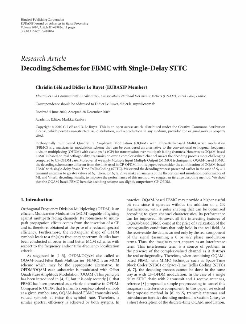
Hindawi Publishing CorporationEURASIP Journal on Advances in Signal ProcessingVolume 2010, Article ID 689824, 11 pagesdoi:10.1155/2010/689824
Research Article
Decoding Schemes for FBMC with Single-Delay STTC
Chrislin Lele and Didier Le Ruyet (EURASIP Member)
Electronics and Communications Laboratory, Conservatoire National Des Arts Et Metiers (CNAM), 75141 Paris, France
Correspondence should be addressed to Didier Le Ruyet, didier.le [email protected]
Received 5 June 2009; Accepted 28 December 2009
Academic Editor: Markku Renfors
Copyright © 2010 C. Lele and D. Le Ruyet. This is an open access article distributed under the Creative Commons AttributionLicense, which permits unrestricted use, distribution, and reproduction in any medium, provided the original work is properlycited.
Orthogonally multiplexed Quadrature Amplitude Modulation (OQAM) with Filter-Bank-based MultiCarrier modulation(FBMC) is a multicarrier modulation scheme that can be considered an alternative to the conventional orthogonal frequencydivision multiplexing (OFDM) with cyclic prefix (CP) for transmission over multipath fading channels. However, as OQAM-basedFBMC is based on real orthogonality, transmission over a complex-valued channel makes the decoding process more challengingcompared to CP-OFDM case. Moreover, if we apply Multiple Input Multiple Output (MIMO) techniques to OQAM-based FBMC,the decoding schemes are different from the ones used in CP-OFDM. In this paper, we consider the combination of OQAM-basedFBMC with single-delay Space-Time Trellis Coding (STTC). We extend the decoding process presented earlier in the case ofNt = 2transmit antennas to greater values of Nt . Then, for Nt ≥ 2, we make an analysis of the theoretical and simulation performance ofML and Viterbi decoding. Finally, to improve the performance of this method, we suggest an iterative decoding method. We showthat the OQAM-based FBMC iterative decoding scheme can slightly outperform CP-OFDM.
1. Introduction
Orthogonal Frequency Division Multiplexing (OFDM) is anefficient Multicarrier Modulation (MCM) capable of fightingagainst multipath fading channels. Its robustness to multi-path propagation effects comes from the insertion of a CPand is, therefore, obtained at the price of a reduced spectralefficiency. Furthermore, the rectangular shape of OFDMsymbols leads to a sin(x)/x frequency spectrum. Studies havebeen conducted in order to find better MCM schemes withrespect to the frequency and/or time-frequency localizationcriteria.
As suggested in [1–3], OFDM/OQAM also called asOQAM-based Filter Bank Multicarrier (FBMC) is an MCMscheme which may be the appropriate alternative. InOFDM/OQAM each subcarrier is modulated with OffsetQuadrature Amplitude Modulation (OQAM). This principlehas been introduced in [4, 5], but it is only recently [1] thatFBMC has been presented as a viable alternative to OFDM.Compared to OFDM that transmits complex-valued symbolsat a given symbol rate, OQAM-based FBMC transmits real-valued symbols at twice this symbol rate. Therefore, asimilar spectral efficiency is achieved by both systems. In
practice, OQAM-based FBMC may provide a higher usefulbit rate since it operates without the addition of a CP.Furthermore, with a pulse shaping that can be optimizedaccording to given channel characteristics, its performancecan be improved. However, all the interesting features ofOQAM-based FBMC come at the price of a relaxation of theorthogonality conditions that only hold in the real field. Atthe receive side the data is carried only by the real componentof the signal (assuming a 0 or π/2 phase modulationterm). Thus, the imaginary part appears as an interferenceterm. This interference term is a source of problem inthe presence of the complex-valued channel as it destroysthe real orthogonality. Therefore, when combining OQAM-based FBMC with MIMO technique such as Space-TimeBlock Codes (STBC) or Space-Time Trellis Coding (STTC)[6, 7], the decoding process cannot be done in the sameway as with CP-OFDM modulation. In the case of a singledelay STTC chain with 2 transmit and 1 receive antennas,refrence [8] proposed a simple preprocessing to cancel thisimaginary interference component. In this paper, we extendthe proposed method in [8] to Nt transmit antennas andintroduce an iterative decoding method. In Section 2, we givea short description of the discrete-time OQAM modulation.
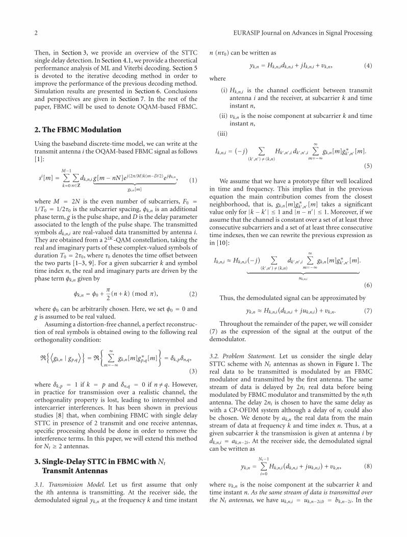
2 EURASIP Journal on Advances in Signal Processing
Then, in Section 3, we provide an overview of the STTCsingle delay detection. In Section 4.1, we provide a theoreticalperformance analysis of ML and Viterbi decoding. Section 5is devoted to the iterative decoding method in order toimprove the performance of the previous decoding method.Simulation results are presented in Section 6. Conclusionsand perspectives are given in Section 7. In the rest of thepaper, FBMC will be used to denote OQAM-based FBMC.
2. The FBMC Modulation
Using the baseband discrete-time model, we can write at thetransmit antenna i the OQAM-based FBMC signal as follows[1]:
si[m] =M−1∑
k=0
∑
n∈Z
dk,n,i g[m− nN]e j(2π/M)k(m−D/2)e jφk,n
︸ ︷︷ ︸gk,n[m]
, (1)
where M = 2N is the even number of subcarriers, F0 =1/T0 = 1/2τ0 is the subcarrier spacing, φk,n is an additionalphase term, g is the pulse shape, andD is the delay parameterassociated to the length of the pulse shape. The transmittedsymbols dk,n,i are real-valued data transmitted by antenna i.They are obtained from a 22K -QAM constellation, taking thereal and imaginary parts of these complex-valued symbols ofduration T0 = 2τ0, where τ0 denotes the time offset betweenthe two parts [1–3, 9]. For a given subcarrier k and symboltime index n, the real and imaginary parts are driven by thephase term φk,n given by
φk,n = φ0 +π
2(n + k) (mod π), (2)
where φ0 can be arbitrarily chosen. Here, we set φ0 = 0 andg is assumed to be real valued.
Assuming a distortion-free channel, a perfect reconstruc-tion of real symbols is obtained owing to the following realorthogonality condition:
R{⟨gk,n | gp,q
⟩}= R
{ ∞∑
m=−∞gk,n[m]g∗p,q[m]
}= δk,pδn,q,
(3)
where δk,p = 1 if k = p and δn,q = 0 if n /= q. However,in practice for transmission over a realistic channel, theorthogonality property is lost, leading to intersymbol andintercarrier interferences. It has been shown in previousstudies [8] that, when combining FBMC with single delaySTTC in presence of 2 transmit and one receive antennas,specific processing should be done in order to remove theinterference terms. In this paper, we will extend this methodfor Nt ≥ 2 antennas.
3. Single-Delay STTC in FBMC with Nt
Transmit Antennas
3.1. Transmission Model. Let us first assume that onlythe ith antenna is transmitting. At the receiver side, thedemodulated signal yk,n at the frequency k and time instant
n (nτ0) can be written as
yk,n = Hk,n,idk,n,i + jIk,n,i + υk,n, (4)
where
(i) Hk,n,i is the channel coefficient between transmitantenna i and the receiver, at subcarrier k and timeinstant n,
(ii) υk,n is the noise component at subcarrier k and timeinstant n,
(iii)
Ik,n,i =(− j)
∑
(k′,n′) /= (k,n)
Hk′,n′,i dk′,n′,i
∞∑
m=−∞gk,n[m]g∗k′,n′[m].
(5)
We assume that we have a prototype filter well localizedin time and frequency. This implies that in the previousequation the main contribution comes from the closestneighborhood, that is, gk,n[m]g∗k′,n′[m] takes a significantvalue only for |k − k′| ≤ 1 and |n− n′| ≤ 1. Moreover, if weassume that the channel is constant over a set of at least threeconsecutive subcarriers and a set of at least three consecutivetime indexes, then we can rewrite the previous expression asin [10]:
Ik,n,i ≈ Hk,n,i(− j)
∑
(k′,n′) /= (k,n)
dk′,n′,i
∞∑
m=−∞gk,n[m]g∗k′,n′[m]
︸ ︷︷ ︸uk,n,i
.
(6)
Thus, the demodulated signal can be approximated by
yk,n ≈ Hk,n,i(dk,n,i + juk,n,i
)+ υk,n. (7)
Throughout the remainder of the paper, we will consider(7) as the expression of the signal at the output of thedemodulator.
3.2. Problem Statement. Let us consider the single delaySTTC scheme with Nt antennas as shown in Figure 1. Thereal data to be transmitted is modulated by an FBMCmodulator and transmitted by the first antenna. The samestream of data is delayed by 2ni real data before beingmodulated by FBMC modulator and transmitted by the nithantenna. The delay 2ni is chosen to have the same delay aswith a CP-OFDM system although a delay of ni could alsobe chosen. We denote by ak,n the real data from the mainstream of data at frequency k and time index n. Thus, at agiven subcarrier k the transmission is given at antenna i bydk,n,i = ak,n−2i. At the receiver side, the demodulated signalcan be written as
yk,n =Nt−1∑
i=0
Hk,n,i(dk,n,i + juk,n,i
)+ υk,n, (8)
where υk,n is the noise component at the subcarrier k andtime instant n. As the same stream of data is transmitted overthe Nt antennas, we have uk,n,i = uk,n−2i,0 = bk,n−2i. In the
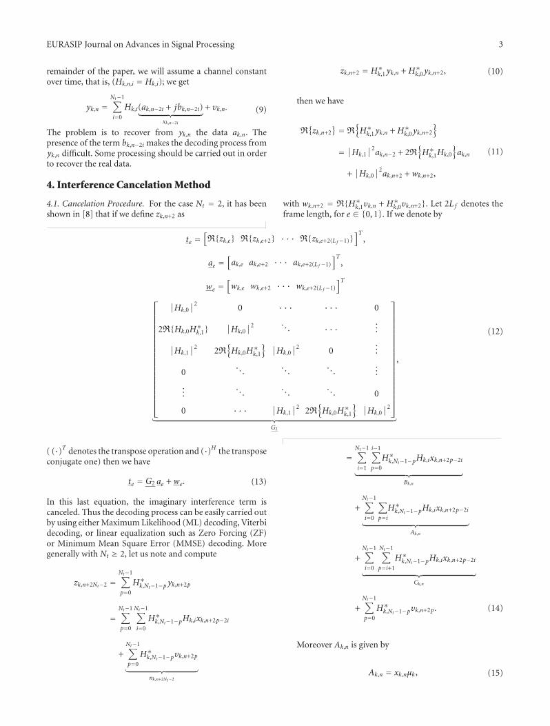
EURASIP Journal on Advances in Signal Processing 3
remainder of the paper, we will assume a channel constantover time, that is, (Hk,n,i = Hk,i); we get
yk,n =Nt−1∑
i=0
Hk,i(ak,n−2i + jbk,n−2i)︸ ︷︷ ︸xk,n−2i
+ υk,n. (9)
The problem is to recover from yk,n the data ak,n. Thepresence of the term bk,n−2i makes the decoding process fromyk,n difficult. Some processing should be carried out in orderto recover the real data.
4. Interference Cancelation Method
4.1. Cancelation Procedure. For the case Nt = 2, it has beenshown in [8] that if we define zk,n+2 as
zk,n+2 = H∗k,1yk,n +H∗
k,0yk,n+2, (10)
then we have
R{zk,n+2
} = R{H∗k,1yk,n +H∗
k,0yk,n+2
}
= ∣∣Hk,1∣∣2ak,n−2 + 2R
{H∗k,1Hk,0
}ak,n
+∣∣Hk,0
∣∣2ak,n+2 +wk,n+2,
(11)
with wk,n+2 = R{H∗k,1υk,n + H∗
k,0υk,n+2}. Let 2L f denotes theframe length, for e ∈ {0, 1}. If we denote by
te =[R{zk,e} R{zk,e+2} · · · R{zk,e+2(L f−1)}
]T,
ae =[ak,e ak,e+2 · · · ak,e+2(L f −1)
]T,
we =[wk,e wk,e+2 · · · wk,e+2(L f−1)
]T
⎡⎢⎢⎢⎢⎢⎢⎢⎢⎢⎢⎢⎢⎢⎢⎢⎢⎢⎢⎢⎣
∣∣Hk,0∣∣2 0 · · · · · · 0
2R{Hk,0H∗k,1}
∣∣Hk,0∣∣2 . . . · · ·
...
∣∣Hk,1∣∣2 2R
{Hk,0H
∗k,1
} ∣∣Hk,0∣∣2 0
...
0. . .
. . .. . .
...
.... . .
. . .. . . 0
0 · · · ∣∣Hk,1∣∣2 2R
{Hk,0H
∗k,1
} ∣∣Hk,0∣∣2
⎤⎥⎥⎥⎥⎥⎥⎥⎥⎥⎥⎥⎥⎥⎥⎥⎥⎥⎥⎥⎦
︸ ︷︷ ︸G2
,
(12)
( (·)T denotes the transpose operation and (·)H the transposeconjugate one) then we have
te = G2 ae +we. (13)
In this last equation, the imaginary interference term iscanceled. Thus the decoding process can be easily carried outby using either Maximum Likelihood (ML) decoding, Viterbidecoding, or linear equalization such as Zero Forcing (ZF)or Minimum Mean Square Error (MMSE) decoding. Moregenerally with Nt ≥ 2, let us note and compute
zk,n+2Nt−2 =Nt−1∑
p=0
H∗k,Nt−1−p yk,n+2p
=Nt−1∑
p=0
Nt−1∑
i=0
H∗k,Nt−1−pHk,ixk,n+2p−2i
+Nt−1∑
p=0
H∗k,Nt−1−pυk,n+2p
︸ ︷︷ ︸nk,n+2Nt−2
=Nt−1∑
i=1
i−1∑
p=0
H∗k,Nt−1−pHk,ixk,n+2p−2i
︸ ︷︷ ︸Bk,n
+Nt−1∑
i=0
∑
p=iH∗k,Nt−1−pHk,ixk,n+2p−2i
︸ ︷︷ ︸Ak,n
+Nt−1∑
i=0
Nt−1∑
p=i+1
H∗k,Nt−1−pHk,ixk,n+2p−2i
︸ ︷︷ ︸Ck,n
+Nt−1∑
p=0
H∗k,Nt−1−pυk,n+2p. (14)
Moreover Ak,n is given by
Ak,n = xk,nμk, (15)
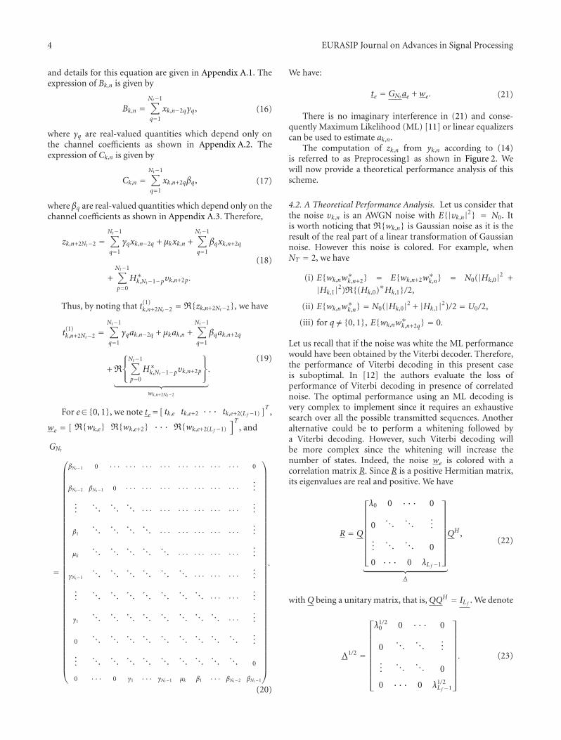
4 EURASIP Journal on Advances in Signal Processing
and details for this equation are given in Appendix A.1. Theexpression of Bk,n is given by
Bk,n =Nt−1∑
q=1
xk,n−2qγq, (16)
where γq are real-valued quantities which depend only onthe channel coefficients as shown in Appendix A.2. Theexpression of Ck,n is given by
Ck,n =Nt−1∑
q=1
xk,n+2qβq, (17)
where βq are real-valued quantities which depend only on thechannel coefficients as shown in Appendix A.3. Therefore,
zk,n+2Nt−2 =Nt−1∑
q=1
γqxk,n−2q + μkxk,n +Nt−1∑
q=1
βqxk,n+2q
+Nt−1∑
p=0
H∗k,Nt−1−pυk,n+2p.
(18)
Thus, by noting that t(1)k,n+2Nt−2 = R{zk,n+2Nt−2}, we have
t(1)k,n+2Nt−2 =
Nt−1∑
q=1
γqak,n−2q + μkak,n +Nt−1∑
q=1
βqak,n+2q
+ R
⎧⎨⎩
Nt−1∑
p=0
H∗k,Nt−1−pυk,n+2p
⎫⎬⎭
︸ ︷︷ ︸wk,n+2Nt−2
.(19)
For e∈{0, 1}, we note te=[ tk,e tk,e+2 · · · tk,e+2(L f −1) ]T
,
we = [ R{wk,e} R{wk,e+2} · · · R{wk,e+2(L f −1)
]T, and
GNt
=
⎛⎜⎜⎜⎜⎜⎜⎜⎜⎜⎜⎜⎜⎜⎜⎜⎜⎜⎜⎜⎜⎜⎜⎜⎜⎜⎜⎜⎜⎜⎜⎜⎜⎜⎜⎜⎜⎜⎜⎜⎜⎜⎝
βNt−1 0 · · · · · · · · · · · · · · · · · · · · · · · · 0
βNt−2 βNt−1 0 · · · · · · · · · · · · · · · · · · · · ·...
.... . .
. . .. . . · · · · · · · · · · · · · · · · · ·
...
β1
. . .. . .
. . .. . . · · · · · · · · · · · · · · ·
...
μk. . .
. . .. . .
. . .. . . · · · · · · · · · · · ·
...
γNt−1
. . .. . .
. . .. . .
. . .. . . · · · · · · · · ·
...
.... . .
. . .. . .
. . .. . .
. . .. . . · · · · · ·
...
γ1
. . .. . .
. . .. . .
. . .. . .
. . .. . . · · ·
...
0.. .
. . .. . .
. . .. . .
. . .. . .
. . .. . .
...
.... . .
. . .. . .
. . .. . .
. . .. . .
. . .. . . 0
0 · · · 0 γ1 · · · γNt−1 μk β1 · · · βNt−2 βNt−1
⎞⎟⎟⎟⎟⎟⎟⎟⎟⎟⎟⎟⎟⎟⎟⎟⎟⎟⎟⎟⎟⎟⎟⎟⎟⎟⎟⎟⎟⎟⎟⎟⎟⎟⎟⎟⎟⎟⎟⎟⎟⎟⎠
.
(20)
We have:
te = GNtae +we. (21)
There is no imaginary interference in (21) and conse-quently Maximum Likelihood (ML) [11] or linear equalizerscan be used to estimate ak,n.
The computation of zk,n from yk,n according to (14)is referred to as Preprocessing1 as shown in Figure 2. Wewill now provide a theoretical performance analysis of thisscheme.
4.2. A Theoretical Performance Analysis. Let us consider thatthe noise υk,n is an AWGN noise with E{|υk,n|2} = N0. Itis worth noticing that R{wk,n} is Gaussian noise as it is theresult of the real part of a linear transformation of Gaussiannoise. However this noise is colored. For example, whenNT = 2, we have
(i) E{wk,nw∗k,n+2} = E{wk,n+2w
∗k,n} = N0(|Hk,0|2 +
|Hk,1|2)R{(Hk,0)∗Hk,1}/2,
(ii) E{wk,nw∗k,n} = N0(|Hk,0|2 + |Hk,1|2)/2 = U0/2,
(iii) for q /={0, 1}, E{wk,nw∗k,n+2q} = 0.
Let us recall that if the noise was white the ML performancewould have been obtained by the Viterbi decoder. Therefore,the performance of Viterbi decoding in this present caseis suboptimal. In [12] the authors evaluate the loss ofperformance of Viterbi decoding in presence of correlatednoise. The optimal performance using an ML decoding isvery complex to implement since it requires an exhaustivesearch over all the possible transmitted sequences. Anotheralternative could be to perform a whitening followed bya Viterbi decoding. However, such Viterbi decoding willbe more complex since the whitening will increase thenumber of states. Indeed, the noise we is colored with acorrelation matrix R. Since R is a positive Hermitian matrix,its eigenvalues are real and positive. We have
R = Q
⎡⎢⎢⎢⎢⎢⎢⎢⎢⎣
λ0 0 · · · 0
0. . .
. . ....
.... . .
. . . 0
0 · · · 0 λLf −1
⎤⎥⎥⎥⎥⎥⎥⎥⎥⎦
︸ ︷︷ ︸Λ
QH ,(22)
withQ being a unitary matrix, that is,QQH = IL f . We denote
Λ1/2 =
⎡⎢⎢⎢⎢⎢⎢⎢⎢⎢⎣
λ1/20 0 · · · 0
0. . .
. . ....
.... . .
. . . 0
0 · · · 0 λ1/2L f −1
⎤⎥⎥⎥⎥⎥⎥⎥⎥⎥⎦
. (23)
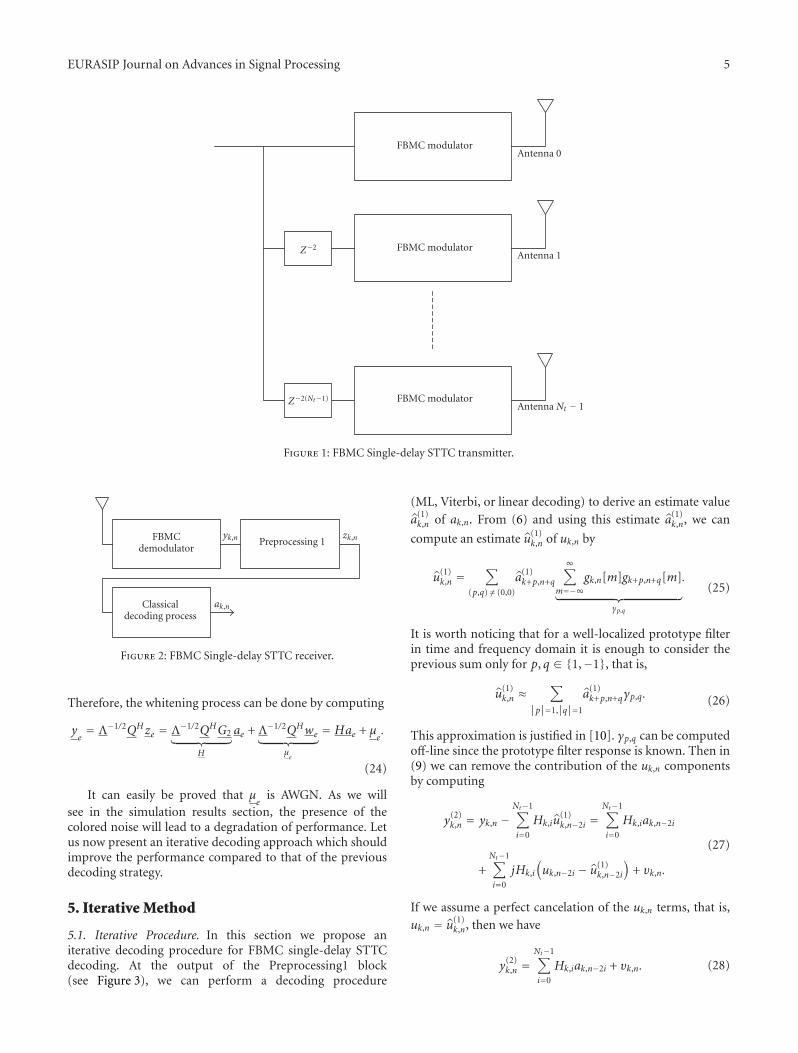
EURASIP Journal on Advances in Signal Processing 5
FBMC modulator
FBMC modulator
FBMC modulator
Z−2
Antenna 0
Antenna 1
Z−2(Nt−1)Antenna Nt − 1
Figure 1: FBMC Single-delay STTC transmitter.
FBMCdemodulator
Preprocessing 1yk,n zk,n
Classicaldecoding process
ak,n
Figure 2: FBMC Single-delay STTC receiver.
Therefore, the whitening process can be done by computing
ye= Λ−1/2QHze = Λ−1/2QHG2︸ ︷︷ ︸
H
ae +Λ−1/2QHwe︸ ︷︷ ︸μe
= Hae + μe.
(24)
It can easily be proved that μe
is AWGN. As we willsee in the simulation results section, the presence of thecolored noise will lead to a degradation of performance. Letus now present an iterative decoding approach which shouldimprove the performance compared to that of the previousdecoding strategy.
5. Iterative Method
5.1. Iterative Procedure. In this section we propose aniterative decoding procedure for FBMC single-delay STTCdecoding. At the output of the Preprocessing1 block(see Figure 3), we can perform a decoding procedure
(ML, Viterbi, or linear decoding) to derive an estimate value
a(1)k,n of ak,n. From (6) and using this estimate a(1)
k,n, we can
compute an estimate u(1)k,n of uk,n by
u(1)k,n =
∑
(p,q) /= (0,0)
a(1)k+p,n+q
∞∑
m=−∞gk,n[m]gk+p,n+q[m]
︸ ︷︷ ︸γp,q
.(25)
It is worth noticing that for a well-localized prototype filterin time and frequency domain it is enough to consider theprevious sum only for p, q ∈ {1,−1}, that is,
u(1)k,n ≈
∑
|p|=1,|q|=1
a(1)k+p,n+qγp,q. (26)
This approximation is justified in [10]. γp,q can be computedoff-line since the prototype filter response is known. Then in(9) we can remove the contribution of the uk,n componentsby computing
y(2)k,n = yk,n −
Nt−1∑
i=0
Hk,iu(1)k,n−2i =
Nt−1∑
i=0
Hk,iak,n−2i
+Nt−1∑
i=0
jHk,i
(uk,n−2i − u(1)
k,n−2i
)+ υk,n.
(27)
If we assume a perfect cancelation of the uk,n terms, that is,uk,n = u(1)
k,n, then we have
y(2)k,n =
Nt−1∑
i=0
Hk,iak,n−2i + υk,n. (28)
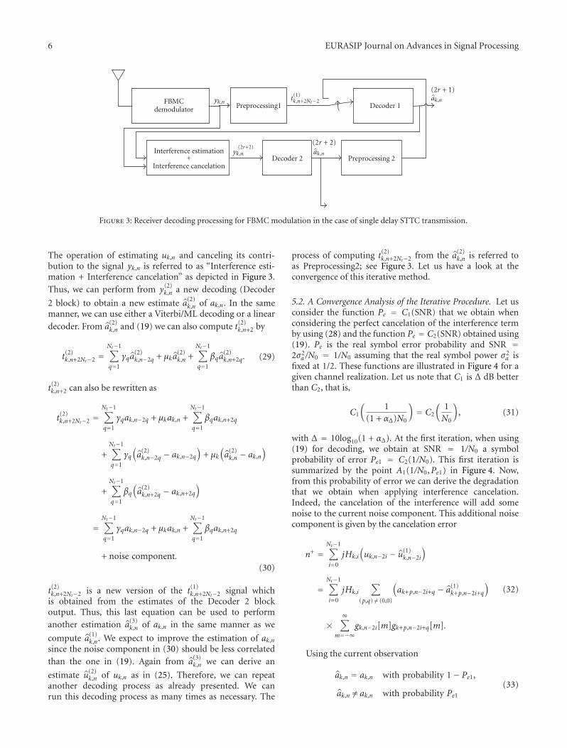
6 EURASIP Journal on Advances in Signal Processing
FBMCdemodulator Preprocessing1 Decoder 1
Decoder 2Interference estimation
+Interference cancelation
Preprocessing 2
yk,nt(1)k,n+2Nt−2
(2r + 1)ak,n
(2r+2)yk,n
(2r + 2)ak,n
Figure 3: Receiver decoding processing for FBMC modulation in the case of single delay STTC transmission.
The operation of estimating uk,n and canceling its contri-bution to the signal yk,n is referred to as “Interference esti-mation + Interference cancelation” as depicted in Figure 3.
Thus, we can perform from y(2)k,n a new decoding (Decoder
2 block) to obtain a new estimate a(2)k,n of ak,n. In the same
manner, we can use either a Viterbi/ML decoding or a linear
decoder. From a(2)k,n and (19) we can also compute t(2)
k,n+2 by
t(2)k,n+2Nt−2 =
Nt−1∑
q=1
γqa(2)k,n−2q + μka
(2)k,n +
Nt−1∑
q=1
βqa(2)k,n+2q. (29)
t(2)k,n+2 can also be rewritten as
t(2)k,n+2Nt−2 =
Nt−1∑
q=1
γqak,n−2q + μkak,n +Nt−1∑
q=1
βqak,n+2q
+Nt−1∑
q=1
γq(a(2)k,n−2q − ak,n−2q
)+ μk
(a(2)k,n − ak,n
)
+Nt−1∑
q=1
βq(a(2)k,n+2q − ak,n+2q
)
=Nt−1∑
q=1
γqak,n−2q + μkak,n +Nt−1∑
q=1
βqak,n+2q
+ noise component.(30)
t(2)k,n+2Nt−2 is a new version of the t(1)
k,n+2Nt−2 signal whichis obtained from the estimates of the Decoder 2 blockoutput. Thus, this last equation can be used to performanother estimation a(3)
k,n of ak,n in the same manner as we
compute a(1)k,n. We expect to improve the estimation of ak,n
since the noise component in (30) should be less correlatedthan the one in (19). Again from a(3)
k,n we can derive an
estimate u(2)k,n of uk,n as in (25). Therefore, we can repeat
another decoding process as already presented. We canrun this decoding process as many times as necessary. The
process of computing t(2)k,n+2Nt−2 from the a(2)
k,n is referred toas Preprocessing2; see Figure 3. Let us have a look at theconvergence of this iterative method.
5.2. A Convergence Analysis of the Iterative Procedure. Let usconsider the function Pe = C1(SNR) that we obtain whenconsidering the perfect cancelation of the interference termby using (28) and the function Pe = C2(SNR) obtained using(19). Pe is the real symbol error probability and SNR =2σ2
a /N0 = 1/N0 assuming that the real symbol power σ2a is
fixed at 1/2. These functions are illustrated in Figure 4 for agiven channel realization. Let us note that C1 is Δ dB betterthan C2, that is,
C1
(1
(1 + αΔ)N0
)= C2
(1N0
), (31)
with Δ = 10log10(1 + αΔ). At the first iteration, when using(19) for decoding, we obtain at SNR = 1/N0 a symbolprobability of error Pe1 = C2(1/N0). This first iteration issummarized by the point A1(1/N0,Pe1) in Figure 4. Now,from this probability of error we can derive the degradationthat we obtain when applying interference cancelation.Indeed, the cancelation of the interference will add somenoise to the current noise component. This additional noisecomponent is given by the cancelation error
n+ =Nt−1∑
i=0
jHk,i
(uk,n−2i − u(1)
k,n−2i
)
=Nt−1∑
i=0
jHk,i
∑
(p,q) /= (0,0)
(ak+p,n−2i+q − a(1)
k+p,n−2i+q
)
×∞∑
m=−∞gk,n−2i[m]gk+p,n−2i+q[m].
(32)
Using the current observation
ak,n = ak,n with probability 1− Pe1,
ak,n /= ak,n with probability Pe1(33)
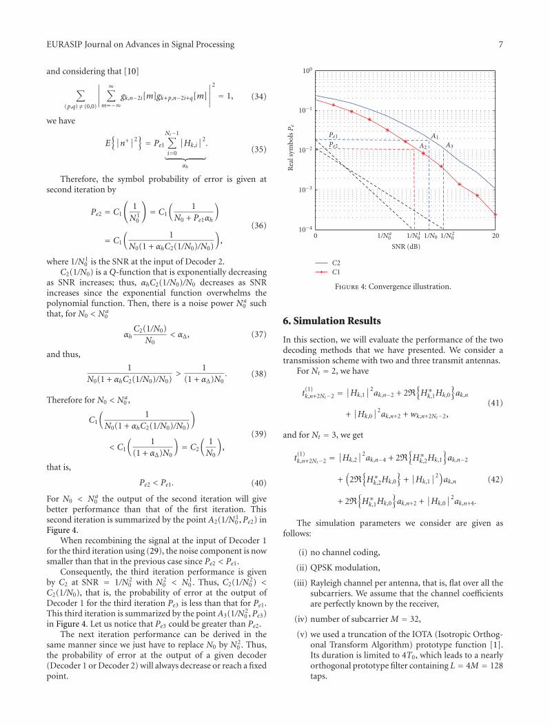
EURASIP Journal on Advances in Signal Processing 7
and considering that [10]
∑
(p,q) /= (0,0)
∣∣∣∣∣
∞∑
m=−∞gk,n−2i[m]gk+p,n−2i+q[m]
∣∣∣∣∣
2
= 1, (34)
we have
E{∣∣n+
∣∣2}= Pe1
Nt−1∑
i=0
∣∣Hk,i∣∣2
︸ ︷︷ ︸αh
.(35)
Therefore, the symbol probability of error is given atsecond iteration by
Pe2 = C1
(1N1
0
)= C1
(1
N0 + Pe1αh
)
= C1
(1
N0(1 + αhC2(1/N0)/N0)
),
(36)
where 1/N10 is the SNR at the input of Decoder 2.
C2(1/N0) is a Q-function that is exponentially decreasingas SNR increases; thus, αhC2(1/N0)/N0 decreases as SNRincreases since the exponential function overwhelms thepolynomial function. Then, there is a noise power Na
0 suchthat, for N0 < N
a0
αhC2(1/N0)
N0< αΔ, (37)
and thus,
1N0(1 + αhC2(1/N0)/N0)
>1
(1 + αΔ)N0. (38)
Therefore for N0 < Na0 ,
C1
(1
N0(1 + αhC2(1/N0)/N0)
)
< C1
(1
(1 + αΔ)N0
)= C2
(1N0
),
(39)
that is,
Pe2 < Pe1. (40)
For N0 < Na0 the output of the second iteration will give
better performance than that of the first iteration. Thissecond iteration is summarized by the point A2(1/N1
0 ,Pe2) inFigure 4.
When recombining the signal at the input of Decoder 1for the third iteration using (29), the noise component is nowsmaller than that in the previous case since Pe2 < Pe1.
Consequently, the third iteration performance is givenby C2 at SNR = 1/N2
0 with N20 < N1
0 . Thus, C2(1/N20 ) <
C2(1/N0), that is, the probability of error at the output ofDecoder 1 for the third iteration Pe3 is less than that for Pe1.This third iteration is summarized by the point A3(1/N2
0 ,Pe3)in Figure 4. Let us notice that Pe3 could be greater than Pe2.
The next iteration performance can be derived in thesame manner since we just have to replace N0 by N2
0 . Thus,the probability of error at the output of a given decoder(Decoder 1 or Decoder 2) will always decrease or reach a fixedpoint.
10−4
10−3
10−2
10−1
100
Pe1Pe2
Rea
lsym
bolsPe
0 1/Na0 1/N1
0 1/N0 1/N20 20
SNR (dB)
A1
A2 A3
C2C1
Figure 4: Convergence illustration.
6. Simulation Results
In this section, we will evaluate the performance of the twodecoding methods that we have presented. We consider atransmission scheme with two and three transmit antennas.
For Nt = 2, we have
t(1)k,n+2Nt−2 =
∣∣Hk,1∣∣2ak,n−2 + 2R
{H∗k,1Hk,0
}ak,n
+∣∣Hk,0
∣∣2ak,n+2 +wk,n+2Nt−2,
(41)
and for Nt = 3, we get
t(1)k,n+2Nt−2 =
∣∣Hk,2∣∣2ak,n−4 + 2R
{H∗k,2Hk,1
}ak,n−2
+(
2R{H∗k,2Hk,0
}+∣∣Hk,1
∣∣2)ak,n
+ 2R{H∗k,1Hk,0
}ak,n+2 +
∣∣Hk,0∣∣2ak,n+4.
(42)
The simulation parameters we consider are given asfollows:
(i) no channel coding,
(ii) QPSK modulation,
(iii) Rayleigh channel per antenna, that is, flat over all thesubcarriers. We assume that the channel coefficientsare perfectly known by the receiver,
(iv) number of subcarrier M = 32,
(v) we used a truncation of the IOTA (Isotropic Orthog-onal Transform Algorithm) prototype function [1].Its duration is limited to 4T0, which leads to a nearlyorthogonal prototype filter containing L = 4M = 128taps.
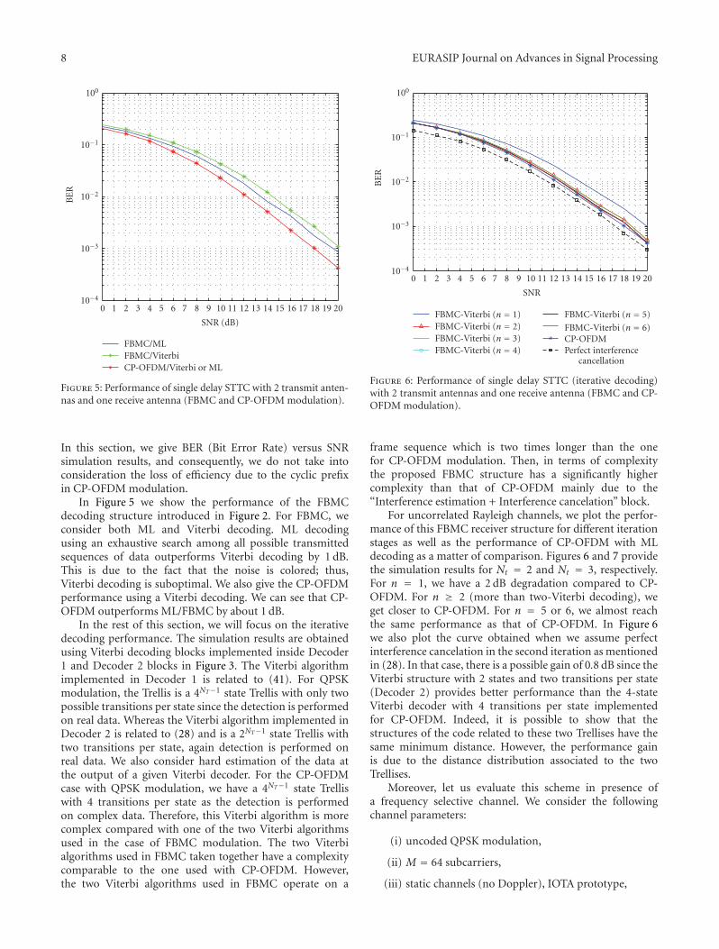
8 EURASIP Journal on Advances in Signal Processing
0 1 2 3 4 5 6 7 8 9 10 11 12 13 14 15 16 17 18 19 20
SNR (dB)
10−4
10−3
10−2
10−1
100
BE
R
FBMC/MLFBMC/ViterbiCP-OFDM/Viterbi or ML
Figure 5: Performance of single delay STTC with 2 transmit anten-nas and one receive antenna (FBMC and CP-OFDM modulation).
In this section, we give BER (Bit Error Rate) versus SNRsimulation results, and consequently, we do not take intoconsideration the loss of efficiency due to the cyclic prefixin CP-OFDM modulation.
In Figure 5 we show the performance of the FBMCdecoding structure introduced in Figure 2. For FBMC, weconsider both ML and Viterbi decoding. ML decodingusing an exhaustive search among all possible transmittedsequences of data outperforms Viterbi decoding by 1 dB.This is due to the fact that the noise is colored; thus,Viterbi decoding is suboptimal. We also give the CP-OFDMperformance using a Viterbi decoding. We can see that CP-OFDM outperforms ML/FBMC by about 1 dB.
In the rest of this section, we will focus on the iterativedecoding performance. The simulation results are obtainedusing Viterbi decoding blocks implemented inside Decoder1 and Decoder 2 blocks in Figure 3. The Viterbi algorithmimplemented in Decoder 1 is related to (41). For QPSKmodulation, the Trellis is a 4NT−1 state Trellis with only twopossible transitions per state since the detection is performedon real data. Whereas the Viterbi algorithm implemented inDecoder 2 is related to (28) and is a 2NT−1 state Trellis withtwo transitions per state, again detection is performed onreal data. We also consider hard estimation of the data atthe output of a given Viterbi decoder. For the CP-OFDMcase with QPSK modulation, we have a 4NT−1 state Trelliswith 4 transitions per state as the detection is performedon complex data. Therefore, this Viterbi algorithm is morecomplex compared with one of the two Viterbi algorithmsused in the case of FBMC modulation. The two Viterbialgorithms used in FBMC taken together have a complexitycomparable to the one used with CP-OFDM. However,the two Viterbi algorithms used in FBMC operate on a
0 1 2 3 4 5 6 7 8 9 10 11 12 13 14 15 16 17 18 19 20
SNR
10−4
10−3
10−2
10−1
100
BE
R
FBMC-Viterbi (n = 1)FBMC-Viterbi (n = 2)FBMC-Viterbi (n = 3)FBMC-Viterbi (n = 4)
FBMC-Viterbi (n = 5)
FBMC-Viterbi (n = 6)CP-OFDMPerfect interference
cancellation
Figure 6: Performance of single delay STTC (iterative decoding)with 2 transmit antennas and one receive antenna (FBMC and CP-OFDM modulation).
frame sequence which is two times longer than the onefor CP-OFDM modulation. Then, in terms of complexitythe proposed FBMC structure has a significantly highercomplexity than that of CP-OFDM mainly due to the“Interference estimation + Interference cancelation” block.
For uncorrelated Rayleigh channels, we plot the perfor-mance of this FBMC receiver structure for different iterationstages as well as the performance of CP-OFDM with MLdecoding as a matter of comparison. Figures 6 and 7 providethe simulation results for Nt = 2 and Nt = 3, respectively.For n = 1, we have a 2 dB degradation compared to CP-OFDM. For n ≥ 2 (more than two-Viterbi decoding), weget closer to CP-OFDM. For n = 5 or 6, we almost reachthe same performance as that of CP-OFDM. In Figure 6we also plot the curve obtained when we assume perfectinterference cancelation in the second iteration as mentionedin (28). In that case, there is a possible gain of 0.8 dB since theViterbi structure with 2 states and two transitions per state(Decoder 2) provides better performance than the 4-stateViterbi decoder with 4 transitions per state implementedfor CP-OFDM. Indeed, it is possible to show that thestructures of the code related to these two Trellises have thesame minimum distance. However, the performance gainis due to the distance distribution associated to the twoTrellises.
Moreover, let us evaluate this scheme in presence ofa frequency selective channel. We consider the followingchannel parameters:
(i) uncoded QPSK modulation,
(ii) M = 64 subcarriers,
(iii) static channels (no Doppler), IOTA prototype,
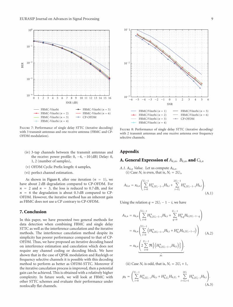
EURASIP Journal on Advances in Signal Processing 9
0 1 2 3 4 5 6 7 8 9 10 11 12 13 14 15 16
SNR (dB)
10−4
10−3
10−2
10−1
100
BE
R
FBMC-ViterbiFBMC-Viterbi (n = 2)FBMC-Viterbi (n = 3)FBMC-Viterbi (n = 4)
FBMC-Viterbi (n = 5)FBMC-Viterbi (n = 6)CP-OFDM
Figure 7: Performance of single delay STTC (iterative decoding)with 3 transmit antennas and one receive antenna (FBMC and CP-OFDM modulation).
(iv) 3-tap channels between the transmit antennas andthe receive: power profile: 0, −4, −10 (dB) Delay: 0,1, 2 (number of samples),
(v) OFDM Cyclic Prefix length: 4 samples,
(vi) perfect channel estimation.
As shown in Figure 8, after one iteration (n = 1), wehave about 2 dB degradation compared to CP-OFDM. Forn = 2 and n = 3, the loss is reduced to 0.7 dB, and forn = 6 the degradation is about 0.3 dB compared to CP-OFDM. However, the iterative method has an inherent gainas FBMC does not use a CP contrary to CP-OFDM.
7. Conclusion
In this paper, we have presented two general methods fordata detection when combining FBMC and single delaySTTC as well as the interference cancelation and the iterativemethods. The interference cancelation method despite itssimplicity has poorer performance compared to that of CP-OFDM. Thus, we have proposed an iterative decoding basedon interference estimation and cancelation which does notrequire any channel coding or decoding block. We haveshown that in the case of QPSK modulation and Rayleigh orfrequency selective channels it is possible with this decodingmethod to perform as better as OFDM-STTC. Moreover ifthe iterative cancelation process is improved, then a potentialgain can be achieved. This is obtained with a relatively highercomplexity. In future work, we will look at FBMC withother STTC schemes and evaluate their performance undernonlocally flat channels.
−6 −5 −4 −3 −2 −1 0 1 2 3 4 5 6
SNR
10−3
10−2
10−1
FBMC/Viterbi (n = 1)FBMC/Viterbi (n = 2)FBMC/Viterbi (n = 3)FBMC/Viterbi (n = 4)
FBMC/Viterbi (n = 5)FBMC/Viterbi (n = 6)CP-OFDM
Figure 8: Performance of single delay STTC (iterative decoding)with 2 transmit antennas and one receive antenna over frequencyselective channels.
Appendix
A. General Expression of Ak,n, Bk,n, and Ck,n
A.1. Ak,n Value. Let us compute Ak,n.(i) Case Nt is even, that is, Nt = 2Ut,
Ak,n = xk,n
⎛⎝Ut−1∑
i=0
H∗k,2Ut−1−iHk,i +
2Ut−1∑
i=Ut
H∗k,2Ut−1−iHk,i
⎞⎠.
(A.1)
Using the relation q = 2Ut − 1− i, we have
Ak,n = xk,n
⎛⎝Ut−1∑
i=0
H∗k,2Ut−1−iHk,i +
Ut−1∑
q=0
H∗k,qHk,2Ut−1−q
⎞⎠
= xk,n
⎛⎝Ut−1∑
i=0
(H∗k,2Ut−1−iHk,i +H∗
k,iHk,2Ut−1−i)⎞⎠
= xk,n
⎛⎝2
Ut−1∑
i=0
R{(H∗k,2Ut−1−iHk,i
)}⎞⎠
︸ ︷︷ ︸μk
.
(A.2)
(ii) Case Nt is odd, that is, Nt = 2Ut + 1,
μk =⎛⎝Ut−1∑
i=0
H∗k,2Ut−iHk,i +H∗
k,UtHk,Ut +
2Ut∑
i=Ut+1
H∗k,2Ut−iHk,i
⎞⎠.
(A.3)

10 EURASIP Journal on Advances in Signal Processing
Again using q = 2Ut − i, we have
μk =⎛⎝2
Ut−1∑
i=0
R{(H∗k,2Ut−iHk,i
)}+∣∣Hk,Ut
∣∣2
⎞⎠, (A.4)
and we get
Ak,n = xk,nμk. (A.5)
A.2. Bk,n Value. Let us now compute Bk,n; setting q = p − i,we get
Bk,n =Nt−1∑
i=1
i−1∑
p=0
H∗k,Nt−1−pHk,ixk,n+2p−2i
=Nt−1∑
i=1
i∑
q=1
xk,n−2qH∗k,Nt−1+q−iHk,i.
(A.6)
This last equation is the sum over a triangular set of index;therefore, the sum can be taken either from lines or fromcolumns where the total is the same. Therefore,
Bk,n =Nt−1∑
q=1
xk,n−2q
Nt−1∑
i=qH∗k,Nt−1+q−iHk,i. (A.7)
Taking m = i− q, we get
Bk,n =Nt−1∑
q=1
xk,n−2q
Nt−1−q∑
m=0
H∗k,Nt−1−mHk,m+q
︸ ︷︷ ︸γq
.(A.8)
(i) Case Nt − q is even, that is, Nt − q = 2Uq; then,
γq =Nt−1−q∑
m=0
H∗k,Nt−1−mHk,m+q
=Uq−1∑
m=0
H∗k,2Uq+q−1−mHk,m+q
+2Uq−1∑
m=Uq
H∗k,2Uq+q−1−mHk,m+q
= 2Uq−1∑
m=0
R{H∗k,2Uq+q−1−mHk,m+q
}.
(A.9)
(ii) Case Nt − q is odd, that is, Nt − q = 2Uq + 1; then,
γq =Nt−1−q∑
m=0
H∗k,Nt−1−mHk,m+q
=Uq−1∑
m=0
H∗k,2Uq+q−mHk,m+q +H∗
k,Uq+qHk,Uq+q
+2Uq∑
m=Uq+1
H∗k,2Uq+q−mHk,m+q
= 2Uq−1∑
m=0
R{H∗k,2Uq+q−mHk,m+q
}+∣∣∣H∗
k,Uq+q
∣∣∣2.
(A.10)
A.3. Ck,n Value. Let us now compute Ck,n; setting q = p − i,we get
Ck,n =Nt−2∑
i=1
Nt−1−i∑
q=1
H∗k,Nt−1−q−iHk,ixk,n+2q. (A.11)
This last equation is the sum over a triangular set of index;therefore, the sum can be taken either from lines or fromcolumns where the total is the same. Therefore,
Ck,n =Nt−1∑
q=1
xk,n+2q
Nt−1−q∑
i=0
H∗k,Nt−1−q−iHk,i
︸ ︷︷ ︸βq
.(A.12)
(i) Case Nt − q is even, that is, Nt − q = 2Uq; then,
βq =Nt−1−q∑
i=0
H∗k,Nt−1−q−iHk,i
=Uq−1∑
i=0
H∗k,2Uq−1−iHk,i +
2Uq−1∑
m=Uq
H∗k,2Uq−1−iHk,i
= 2Uq−1∑
i=0
R{H∗k,2Uq−1−iHk,i
}.
(A.13)
(ii) Case Nt − q is odd, that is, Nt − q = 2Uq + 1; then,
βq =Nt−1−q∑
i=0
H∗k,Nt−1−q−iHk,i =
Uq−1∑
i=0
H∗k,2Uq−iHk,i +H∗
k,UqHk,Uq
+2Uq∑
m=Uq+1
H∗k,2Uq−iHk,i
= 2Uq−1∑
m=0
R{H∗k,2Uq−iHk,i
}+∣∣∣H∗
k,Uq
∣∣∣2.
(A.14)
Acknowledgments
The authors would like to thank Pr. M. Bellanger forhelpful discussions. This work was supported in part by theEuropean Commission under Project PHYDYAS (FP7-ICT-2007-1-211887).
References
[1] B. Le Floch, M. Alard, and C. Berrou, “Coded orthogonalfrequency division multiplex,” Proceedings of the IEEE, vol. 83,pp. 982–996, 1995.
[2] H. Boelcskei, “Orthogonal frequency division multiplexingbased on offset QAM,” in Advances in Gabor Analysis,Birkhauser, Boston, Mass, USA, 2003.
[3] P. Siohan, C. Siclet, and N. Lacaille, “Analysis and designof OFDM/OQAM systems based on filterbank theory,” IEEETransactions on Signal Processing, vol. 50, no. 5, pp. 1170–1183,2002.
EURASIP Journal on Advances in Signal Processing 11
[4] R. W. Chang, “Synthesis of band-limited orthogonal signalsfor multi-channel data transmission,” Bell Labs TechnicalJournal, vol. 45, pp. 1775–1796, 1966.
[5] B. R. Saltzberg, “Performance of an efficient parallel datatransmission system,” IEEE Transactions on CommunicationTechnology, vol. 15, no. 6, pp. 805–811, 1967.
[6] V. Tarokh, N. Seshadri, and A. R. Calderbank, “Space-timecodes for high data rate wireless communication: performancecriterion and code construction,” IEEE Transactions on Infor-mation Theory, vol. 44, no. 2, pp. 744–765, 1998.
[7] V. Tarokh, H. Jafarkhani, and A. R. Calderbank, “Space-time block coding for wireless communications: performanceresults,” IEEE Journal on Selected Areas in Communications,vol. 17, no. 3, pp. 451–460, 1999.
[8] M. Bellanger, “Transmit diversity in multicarrier transmissionusing OQAM modulation,” in Proceedings of the 3rd Interna-tional Symposium on Wireless Pervasive Computing (ISWPC’08), pp. 727–730, Santorini, Greece, May 2008.
[9] B. Hirosaki, “Orthogonally multiplexed QAM system usingthe discrete Fourier transform,” IEEE Transactions on Commu-nications Systems, vol. 29, no. 7, pp. 982–989, 1981.
[10] C. Lele, P. Siohan, R. Legouable, and J.-P. Javaudin, “Preamble-based channel estimation techniques for OFDM/OQAM overthe powerline,” in Proceedings of IEEE International Sym-posium on Power Line Communications and Its Applications(ISPLC ’07), pp. 59–64, Pisa, Italy, March 2007.
[11] G. D. Forney Jr., “Maximum-likelihood sequence estimationof digital sequences in the presence of intersymbol interfer-ence,” IEEE Transactions on Information Theory, vol. 18, no. 3,pp. 363–378, 1972.
[12] J.-D. Wang and H. Y. Chung, “Trellis coded communicationsystems in the presence of colored noise: performance analysis,simulation, and the swapping technique,” in Proceeingds ofIEEE Conference Record on Global Telecommunications Con-ference, and Exhibition. ‘Communications for the InformationAge’ (GLOBECOM ’88), vol. 2, pp. 1160–1165, Hollywood, Fla,USA, November-December 1988.

Hindawi Publishing CorporationEURASIP Journal on Advances in Signal ProcessingVolume 2010, Article ID 703513, 13 pagesdoi:10.1155/2010/703513
Research Article
The Alamouti Scheme with CDMA-OFDM/OQAM
Chrislin Lele,1 Pierre Siohan,2 and Rodolphe Legouable2
1 CNAM, Laetitia group, 292, rue Saint Martin, 75141 Paris, France2 Orange Labs, 4, rue du Clos Courtel, BP 91226, 35512 Cesson Sevigne Cedex, France
Correspondence should be addressed to Pierre Siohan, [email protected]
Received 23 June 2009; Revised 4 October 2009; Accepted 29 December 2009
Academic Editor: Behrouz Farhang-Boroujeny
Copyright © 2010 Chrislin Lele et al. This is an open access article distributed under the Creative Commons Attribution License,which permits unrestricted use, distribution, and reproduction in any medium, provided the original work is properly cited.
This paper deals with the combination of OFDM/OQAM with the Alamouti scheme. After a brief presentation of theOFDM/OQAM modulation scheme, we introduce the fact that the well-known Alamouti decoding scheme cannot besimply applied to this modulation. Indeed, the Alamouti coding scheme requires a complex orthogonality property; whereasOFDM/OQAM only provides real orthogonality. However, as we have recently shown, under some conditions, a transmissionscheme combining CDMA and OFDM/OQAM can satisfy the complex orthogonality condition. Adding a CDMA component canthus be seen as a solution to apply the Alamouti scheme in combination with OFDM/OQAM. However, our analysis shows thatthe CDMA-OFDM/OQAM combination has to be built taking into account particular features of the transmission channel. Oursimulation results illustrate the 2× 1 Alamouti coding scheme for which CDMA-OFDM/OQAM and CP-OFDM are compared intwo different scenarios: (i) CDMA is performed in the frequency domain, (ii) CDMA is performed in time domain.
1. Introduction
Increasing the transmission rate and/or providing robustnessto channel conditions are nowadays two of the main researchtopics for wireless communications. Indeed, much effortis done in the area of multiantennas, where Space TimeCodes (STCs) enable to exploit the spatial diversity whenusing several antennas either at the transmitting side orat the receiving side. One of the most known and usedSTC technique is Alamouti code [1]. Alamouti code hasthe nice property to be simple to implement while provid-ing the maximum channel diversity. On the other hand,multicarrier modulation (MCM) is becoming, mainly withthe popular Orthogonal Frequency Division Multiplexing(OFDM) scheme, the appropriate modulation for transmis-sion over frequency selective channels. Furthermore, whenappending the OFDM symbols with a Cyclic Prefix (CP)longer than the maximum delay spread of the channel topreserve the orthogonality, CP-OFDM has the capacity totransform a frequency selective channel into a bunch of flatfading channels which naturally leads to various efficientcombinations of the STC and CP-OFDM schemes. However,the insertion of the CP yields spectral efficiency loss. Inaddition, the conventional OFDM modulation is based on
a rectangular windowing in the time domain which leads toa poor (sinc(x)) behavior in the frequency domain. Thus CP-OFDM gives rise to two drawbacks: loss of spectral efficiencyand sensitivity to frequency dispersion, for example, Dopplerspread.
These two strong limitations may be overcome by someother OFDM variants that also use the exponential baseof functions. But then, in any case, as it can be deducedfrom the Balian-Low theorem, see, for example, [2], it is notpossible to get at the same time (i) Complex orthogonality;(ii) Maximum spectral efficiency; (iii) A well-localized pulseshape in time and frequency. With CP-OFDM conditions(ii) and (iii) are not satisfied, while there are two mainalternatives that satisfy two of these three requirementsand can be implemented as filter bank-based multicarrier(FBMC) modulations. Relaxing condition (ii) we get amodulation scheme named Filtered MultiTone (FMT) [3],also named oversampled OFDM in [4], where the authorsshow that the baseband implementation scheme can be seenas the dual of an oversampled filter bank. But if one reallywants to avoid the two drawbacks of CP-OFDM the onlysolution is to relax the complex orthogonality constraint. Thetransmission system proposed in [5] is a pioneering workthat illustrates this possibility. Later on an efficient Discrete

2 EURASIP Journal on Advances in Signal Processing
Fourier Transform (DFT) implementation of the Saltzbergsystem [5], named Orthogonally Quadrature AmplitudeModulation (O-QAM), has been proposed by Hirosaki [6].To the best of our knowledge, the acronym OFDM/OQAM,where OQAM now corresponds to Offset QAM, appearedfor the first time in [7]. In [7] the authors also present aninvention of Alard, named Isotropic Orthogonal TransformAlgorithm (IOTA), and explicitly use a real inner productto prove the orthogonality of the OFDM/OQAM-IOTAmodem. A formal link between these continuous-time mod-ulation models and a precise filter bank implementation,the Modified Discrete Fourier Transform (MDFT) [8], isestablished in [9].
It is now recognized in a large number of applications,with cognitive radio being the most recent and importantone [10], that appropriate OFDM/OQAM pulse shapeswhich satisfy conditions (ii) and (iii) can be designed,and these can lead to some advantages over the CP-OFDM. However, most of these publications are related toa single user case and to Single-Input-Single-Output (SISO)systems. On the contrary, only a few results are availableconcerning more general requirements being related either tomultiaccess techniques or multiantenna, that is, of MultipleInput Multiple Output (MIMO) type. In a recent publication[11], we have shown that, under certain conditions, acombination of Coded Division Multiple Access (CDMA)with OFDM/OQAM could be used to provide the complexorthogonal property. On the other hand, it has also beenshown in [12] that spatial multiplexing MIMO could bedirectly applied to OFDM/OQAM. However, in the MIMOcase there is still a problem which has not yet found a fullyfavorable issue: It concerns the combined use of the popularSTBC Alamouti code together with OFDM/OQAM. Basicallythe problem is related to the fact that OFDM/OQAMby construction produces an imaginary interference term.Unfortunately, the processing that can be used in the SISOcase, for cancelling it at the transmitter side (TX) [13]or estimating it at the receiver side (RX) [14], cannotbe successfully extended to the Alamouti coding/decodingscheme. Indeed, the solutions proposed so far are not fullysatisfactory. The Alamouti-like scheme for OFDM/OQAMproposed in [15] complicates the RX and introduces aprocessing delay. The pseudo-Alamouti scheme recentlyintroduced in [16] is less complex but requires the appendingof a CP to the OFDM/OQAM signal which means thatcondition (ii) is no longer satisfied.
The aim of this paper is to take advantage of the orthog-onality property resulting from the CDMA-OFDM/OQAMcombination introduced in [11] to get a new MIMO Alam-outi scheme with OFDM/OQAM. The contents of our paperis as follows. In Section 2, after some general descriptionsof the OFDM/OQAM modulation in Section 2.1 and theMIMO Alamouti scheme in Section 2.2, we will combineboth techniques. However, as we will see in Section 2.3,the MIMO decoding process is very difficult becauseof the orthogonality mismatch between Alamouti andOFDM/OQAM. In Section 3, we propose to combine Alam-outi and CDMA-OFDM/OQAM in order to solve the prob-lem. Indeed, in [11], we have shown that the combination
of CDMA and OFDM/OQAM (CDMA-OFDM/OQAM) canprovide the complex orthogonality property; this interestingproperty is first recalled in Section 3.1. Then, two differentapproaches with Alamouti coding are proposed, by consid-ering either a spreading in the frequency (in Section 3.2)or in the time domain (in Section 4.2). When spreadingin time is considered, 2 strategies of implementing theAlamouti coding are proposed. Some simulation resultsfinally show that, using particular channel assumptions, theAlamouti CDMA-OFDM/OQAM technique achieves similarperformance to the Alamouti CP-OFDM system.
2. OFDM/OQAM and Alamouti
2.1. The OFDM/OQAM Transmultiplexer. The basebandequivalent of a continuous-time multicarrier OFDM/OQAMsignal can be expressed as follows [7]:
s(t) =M−1∑
m=0
∑
n∈Z
am,ng(t − nτ0)e j2πmF0tνm,n︸ ︷︷ ︸gm,n(t)
(1)
with Z the set of integers, M = 2N an even number ofsubcarriers, F0 = 1/T0 = 1/2τ0 the subcarrier spacing, gthe prototype function assumed here to be a real-valued andeven function of time, and νm,n an additional phase term suchthat νm,n = jm+ne jφ0 , where φ0 can be chosen arbitrarily.The transmitted data symbols am,n are real-valued. Theyare obtained from a 22K -QAM constellation, taking the realand imaginary parts of these complex-valued symbols ofduration T0 = 2τ0, where τ0 denotes the time offset betweenthe two parts [2, 6, 7, 9].
Assuming a distortion-free channel, the Perfect Recon-struction (PR) of the real data symbols is obtained owing tothe following real orthogonality condition:
R{⟨gm,n, gp,q
⟩}=R
{∫gm,n(t)g∗p,q(t)dt
}=δm,pδn,q, (2)
where ∗ denotes conjugation, 〈·, ·〉 denotes the innerproduct, and δm,p = 1 if m = p and δm,p = 0 ifm /= p. Otherwise said, for (m,n) /= (p, q), 〈gm,n, gp,q〉 is apure imaginary number. For the sake of brevity, we set〈g〉p,q
m,n = − j〈gm,n, gp,q〉. The orthogonality condition for theprototype filter can also be conveniently expressed using itsambiguity function
Ag(n,m) =∫∞
−∞g(u− nτ0)g(u)e2 jπmF0udu. (3)
It is well-known [7] that to satisfy the orthogonalitycondition (2), the prototype filter should be chosen such thatAg(2n, 2m) = 0 if (n,m) /= (0, 0) and Ag(0, 0) = 1.
In practical implementations, the baseband signal isdirectly generated in discrete time, using the continuous-time signal samples at the critical frequency, that is, withFe = MF0 = 2NF0. Then, based on [9], the discrete-time

EURASIP Journal on Advances in Signal Processing 3
a0,n
a1,n
aM−1,n
Pre
mod
ula
tion
IFFT
Poly
phas
e
P/S S/P
Poly
phas
e
FFT
Post
dem
odu
lati
on
...
...
Re{}Re{}
Re{}OQAM modulator OQAM demodulator
Figure 1: Transmultiplexer scheme for the OFDM/OQAM modulation.
OQAMmodulator
OQAMdemodulator
Channel Equalization
a0,n
aM−1,n
a0,n
aM−1,n
R
R
... ...
Figure 2: The transmission scheme based on OFDM/OQAM.
baseband signal taking the causality constraint into account,is expressed as
s[k] =M−1∑
m=0
∑
n∈Z
am,ng(k − nN)e j2πm(k−(Lg−1)/2)νm,n︸ ︷︷ ︸gm,n[k]
. (4)
The parallel between (1) and (4) shows that the overlap-ping of duration τ0 corresponds to N discrete-time samples.For the sake of simplicity, we will assume that the prototypefilter length, denoted Lg , is such that Lg = bM = 2bN , with bbeing a positive integer. With the discrete time formulation,the real orthogonality condition can also be expressed as:
R{⟨gm,n, gp,q
⟩}=R
⎧⎨⎩∑
k∈Z
gm,n[k]g∗p,q[k]
⎫⎬⎭=δm,pδn,q. (5)
As shown in [9], the OFDM/OQAM modem can berealized using the dual structure of the MDFT filter bank.A simplified description is provided in Figure 1, where it hasto be noted that the premodulation corresponds to a singlemultiplication by an exponential whose argument dependson the phase term νm,n and on the prototype length. Notealso that in this scheme, to transmit QAM symbols of a givenduration, denoted T0, the IFFT block has to be run twicefaster than for CP-OFDM. The polyphase block contains thepolyphase components of the prototype filter g. At the RXside, the dual operations are carried out.
The prototype filter has to be PR, or nearly PR. In thispaper, we use a nearly PR prototype filter, with length Lg =4M, resulting from the discretization of the continuous timefunction named Isotropic Orthogonal Transform Algorithm(IOTA) in [7].
Before being transmitted through a channel the basebandsignal is converted to continuous-time. Thus, in the rest ofthis paper, we present an OFDM/OQAM modulator that
delivers a signal denoted s(t), but keeping in mind that thismodulator corresponds to an FBMC modulator as shown inFigure 1.
The block diagram in Figure 2 illustrates our OFDM/OQAM transmission scheme. Note that compared toFigure 1, here a channel breaks the real orthogonalitycondition thus an equalization must be performed at thereceiver side to restore this orthogonality.
Let us consider a time-varying channel, with maximumdelay spread equal to Δ. We denote it by h(t, τ) in time,and it can also be represented by a complex-valued number
H(c)m,n for subcarrier m at symbol time n. At the receiver
side, the received signal is the summation of the s(t) signalconvolved with the channel impulse response and a noisecomponent η(t). For a locally invariant channel, we candefine a neighborhood, denoted ΩΔm,Δn, around the (m0,n0)position, with
ΩΔm,Δn
={(p, q
),∣∣p∣∣≤Δm,
∣∣q∣∣≤Δn | H(c)
m0+p,n0+q ≈ H(c)m0,n0
},
(6)
and we also define Ω∗Δm,Δn = ΩΔm,Δn − {(0, 0)}.Note also that Δn and Δm are chosen according to the
time and bandwidth coherence of the channel, respectively.Then, assuming g(t−τ−nτ0) ≈ g(t−nτ0), for all τ ∈ [0,Δ],the demodulated signal can be expressed as [13, 14, 17]
y(c)m0,n0
= H(c)m0,n0
(am0,n0 + ja(i)
m0,n0
)+ Jm0,n0 + ηm0,n0 (7)
with ηm0,n0 = 〈η, gm0,n0〉 the noise component, a(i)m0,n0 , the
interference created by the neighbor symbols, given by
a(i)m0,n0
=∑
(p,q)∈Ω∗Δm,Δn
am0+p,n0+q⟨g⟩m0,n0
m0+p,n0+q, (8)

4 EURASIP Journal on Advances in Signal Processing
and Jm0,n0 the interference created by the data symbolsoutside ΩΔm,Δn.
It can be shown that, even for small size neighborhoods,if the prototype function g is well localized in time andfrequency, Jm0,n0 becomes negligible when compared to thenoise term ηm0,n0 . Indeed a good time-frequency localization[7] means that the ambiguity function of g, which is directlyrelated to the 〈g〉m0,n0
m0+p,n0+q terms, is concentrated around itsorigin in the time-frequency plane, that is, only takes smallvalues outside the ΩΔm,Δn region. Thus, the received signalcan be approximated by
y(c)m0,n0
≈ H(c)m0,n0
(am0,n0 + ja(i)
m0,n0
)+ ηm0,n0 . (9)
For the rest of our study, we consider (9) as theexpression of the signal at the output of the OFDM/OQAMdemodulator.
2.2. Alamouti Scheme: General Case. In order to describe theAlamouti scheme [1], let us consider the one-tap channelmodel described as
yk = hk,usk,u + nk, (10)
where, at time instant k, hk,u is the channel gain betweenthe transmit antenna u and the receive antenna and nkis an additive noise. We assume that hk,u is a complex-valued Gaussian random process with unitary variance. Onetransmit antenna and one receive antenna are generallyreferred as SISO model. We consider coherent detection, thatis, we assume that the receiver has a perfect knowledge of hk,u.
The Alamouti scheme is implemented with 2 transmitand one receive antennas. Let us consider s2k and s2k+1 tobe the two symbols to transmit at time (time and frequencyaxis can be permuted in multicarrier modulation.) instants2k and 2k + 1, respectively. At time instant 2k, the antenna 0transmits s2k/
√2 whereas the antenna 1 transmits s2k+1/
√2.
At time instant 2k + 1, the antenna 0 transmits −(s2k+1)∗/√
2whereas the antenna 1 transmits s∗2k/
√2. The 1/
√2 factor is
added to normalize the total transmitted power. The receivedsignal samples at time instants 2k and 2k + 1 are given by
y2k = 1√2
(h2k,0s2k + h2k,1s2k+1
)+ n2k,
y2k+1 = 1√2
(−h2k+1,0(s2k+1)∗ + h2k+1,1(s2k)∗
)+ n2k+1.
(11)
Assuming the channel to be constant between the timeinstants 2k and 2k + 1, we get
⎡⎣y2k
y∗2k+1
⎤⎦ = 1√
2
⎡⎣
h2k,0 h2k,1(h2k,1
)∗ −(h2k,0)∗
⎤⎦
︸ ︷︷ ︸H2k
⎡⎣s2k
s2k+1
⎤⎦ +
⎡⎣n2k
n∗2k+1
⎤⎦.
(12)
Note that H2k is an orthogonal matrix with H2kHH2k =
(1/2)(|h2k,0|2 + |h2k,1|2)I2, where I2 is the identity matrixof size (2, 2) and H stands for the transpose conjugate
operation. Thus, using the Maximum Ratio Combining(MRC) equalization, the estimates s2k and s2k+1 are obtainedas⎡⎣s2k
s2k+1
⎤⎦ =
√2
∣∣h2k,0∣∣2 +
∣∣h2k,1∣∣2
⎡⎣
h∗2k,0 h2k,1(h2k,1
)∗ −(h2k,0)
⎤⎦⎡⎣y2k
y2k+1
⎤⎦
=⎡⎣s2k
s2k+1
⎤⎦ +
⎡⎣μ2k
μ2k+1
⎤⎦,
(13)
where,⎡⎣μ2k
μ2k+1
⎤⎦ =
√2
∣∣h2k,0∣∣2 +
∣∣h2k,1∣∣2
⎡⎣
h∗2k,0 h2k,1(h2k,1
)∗ −(h2k,0)
⎤⎦⎡⎣n2k
n∗2k+1
⎤⎦.
(14)
Since the noise components n2k and n2k+1 are uncorrelated,E(|μ2k|2) = E(|μ2k+1|2) = 2N0/(|h2k,0|2 + |h2k,1|2), whereN0 denotes the monolateral noise density. Thus, assuming aQPSK modulation, based on [18], the bit error probability,denoted pb, is given by
pb = Q
⎛⎜⎝
√√√√(∣∣h2k,0
∣∣2 +∣∣h2k,1
∣∣2
2
)SNRt
⎞⎟⎠, (15)
where SNRt denotes the Signal-to-Noise Ratio (SNR) atthe transmitter side. When the two channel coefficients areuncorrelated, we will have a diversity gain of two [18].
2.3. OFDM/OQAM with Alamouti Scheme. Equation(9) indicates that we can consider the transmissionof OFDM/OQAM on each subcarrier as a flat fadingtransmission. Moreover, recalling that in OFDM/OQAM
each complex data symbol, d(c)m,n, is divided into two real
symbols, R{d(c)m,n} and I{d(c)
m,n}, transmitted at successivetime instants, transmission of a pair of data symbols,according to Alamouti scheme, is organized as follows:
am,2n,0 = R{d(c)m,2n
},
am,2n,1 = R{d(c)m,2n+1
},
am,2n+1,0 = I{d(c)m,2n
},
am,2n+1,1 = I{d(c)m,2n+1
},
am,2n+2,0 = −R
{(d(c)m,2n+1
)∗} = −R{d(c)m,2n+1
}= −am,2n,1,
am,2n+2,1 = R
{(d(c)m,2n
)∗} = R{d(c)m,2n
}= am,2n,0,
am,2n+3,0 = −I
{(d(c)m,2n+1
)∗} = I{d(c)m,2n+1
}= am,2n+1,1,
am,2n+3,1 = I
{(d(c)m,2n
)∗} = −I{d(c)m,2n
}= −am,2n+1,0.
(16)

EURASIP Journal on Advances in Signal Processing 5
We also assume that in OFDM/OQAM the channel gainis a constant between the time instants 2n and 2n + 3. Letus denote the channel gain between the transmit antenna iand the receive antenna at subcarrier m and time instant nby hm,n,i. Therefore, at the single receive antenna we have
ym,2n = hm,2n,0
(am,2n,0 + ja(i)
m,2n,0
)
+ hm,2n,1
(am,2n,1 + ja(i)
m,2n,1
)+ nm,2n,0,
ym,2n+1 = hm,2n,0
(am,2n+1,0 + ja(i)
m,2n+1,0
)
+ hm,2n,1
(am,2n+1,1 + ja(i)
m,2n+1,1
)+ nm,2n+1,1,
ym,2n+2 = hm,2n,0
(am,2n+2,0 + ja(i)
m,2n+2,0
)
+ hm,2n,1
(am,2n+2,1 + ja(i)
m,2n+2,1
)+ nm,2n+2,0,
ym,2n+3 = hm,2n,0
(am,2n+3,0 + ja(i)
m,2n+3,0
)
+ hm,2n,1
(am,2n+3,1 + ja(i)
m,2n+3,1
)+ nm,2n+3,1.
(17)
Setting
zm,2n = ym,2n + j ym,2n+1,
zm,2n+1 = ym,2n+2 + j ym,2n+3,(18)
and using (16), we obtain
zm,2n = hm,2n,0d(c)m,2n + hm,2n,1d
(c)m,2n+1
+ hm,2n,0xm,2n,0 + hm,2n,1xm,2n,1 + κm,2n,0,
zm,2n+1 = −hm,2n,0
(d(c)m,2n+1
)∗+ hm,2n,1
(d(c)m,2n
)∗
−hm,2n,0(xm,2n+2,0
)∗+hm,2n,1(xm,2n+2,1
)∗+κm,2n+2,0,(19)
where,
xm,2n,0 = −a(i)m,2n+1,0 + ja(i)
m,2n,0,
xm,2n,1 = −a(i)m,2n+1,1 + ja(i)
m,2n,1,
κm,2n,0 = nm,2n,0 + jnm,2n+1,0,
κm,2n,0 = nm,2n+2,0 + jnm,2n+3,0,
xm,2n+2,0 = a(i)m,2n+3,0 + ja(i)
m,2n+2,0,
xm,2n+2,1 = −a(i)m,2n+3,1 − ja(i)
m,2n+2,1.
(20)
This results in⎡⎣
zm,2n(zm,2n+1
)∗
⎤⎦
︸ ︷︷ ︸z2n
=⎡⎣
hm,2n,0 hm,2n,1(hm,2n,1
)∗ −(hm,2n,0)∗
⎤⎦
︸ ︷︷ ︸Q2n
⎡⎣d(c)m,2n
d(c)m,2n+1
⎤⎦
︸ ︷︷ ︸d2n
+
⎡⎣hm,2n,0 hm,2n,1 0 0
0 0(hm,2n,1
)∗ −(hm,2n,0)∗
⎤⎦
︸ ︷︷ ︸K2n
×
⎡⎢⎢⎢⎢⎢⎢⎣
xm,2n,0
xm,2n,1
xm,2n+2,0
xm,2n+2,1
⎤⎥⎥⎥⎥⎥⎥⎦
︸ ︷︷ ︸x2n
+
⎡⎣
κm,2n(κm,2n+1
)∗
⎤⎦
︸ ︷︷ ︸κ2n
.
(21)
We note that Q2n is an orthogonal matrix which issimilar to the one found in (12) for the conventional 2 × 1Alamouti scheme. However, the K2nx2n term appears, whichis an interference term due to the fact that OFDM/OQAMhas only a real orthogonality. Therefore, even without noiseand assuming a distortion-free channel, we cannot achievea good error probability since K2nx2n is an inherent “noiseinterference” component that, differently from the oneexpressed in (9), cannot be easily removed. (in a particularcase, where hm,2n,0 = hm,2n,1, one can nevertheless get rid ofthe interference terms.)
To tackle this drawback some research studies are beingcarried out. However, as mentioned in the introduction,the first one [15] significantly increases the RX complexity,while the second one [16] fails to reach the objective oftheoretical maximum spectral efficiency, that is, does notsatisfy condition (ii). The one we propose hereafter is basedon a combination of CDMA with OFDM/OQAM and avoidsthese two shortcomings.
3. CDMA-OFDM/OQAM and Alamouti
3.1. CDMA-OFDM/OQAM. In this section we summarizethe results obtained, assuming a distortion-free channel, in[19] and [11] for CDMA-OFDM/OQAM schemes transmit-ting real and complex data symbols, respectively. Then, weshow how this latter scheme can be used for transmissionover a realistic channel model in conjunction with Alamouticoding.
3.1.1. Transmission of Real Data Symbols. We denote byNc the length of the CDMA code used and assume thatNS = M/Nc is an integer number. Let us denote by cu =[c0,u · · · cNc−1,u]T , where (·)T stands for the transposeoperation, the code used by the uth user. When applyingspreading in the frequency domain such as in pure MC-CDMA (Multi-Carrier-CDMA) [20], for a user u0 at agiven time n0, NS different data are transmitted denotedby: du0,n0,0,du0,n0,1, . . . ,du0,n0,NS−1. Then by spreading with

6 EURASIP Journal on Advances in Signal Processing
x0,n
xM−1,n
Real datadu,n
Spreadingin
frequency OQ
AM
mod
ula
tor
ChannelDespreading
infrequencyO
QA
Mde
mod
ula
tor
Equ
aliz
atio
n Re{}
Im{}
du,n
iu,n
Figure 3: Transmission scheme for the CDMA-OFDM/OQAM system with spreading in frequency of real data.
the cu codes, we get the real symbol am0,n0 transmitted atfrequency m0 and time n0 by
am0,n0 =U−1∑
u=0
cm0/Nc ,udu,n0,m0/Nc�, (22)
where U is the number of users, / the modulo operator,and � the floor operator. From the am0,n0 term, thereconstruction of du,n0,p (for p ∈ [0,NS − 1]) is insuredthanks to the orthogonality of the code, that is, cTu1cu2 =δu1,u2; see [21] for more details. Therefore, noise taken apart,the despreading operator leads to
du,n0,p =Nc−1∑
m=0
cm,uapNC+m,n0 . (23)
In [19], it is shown that, since no CP is inserted, thetransmission of these spread real data (du,n0,p) can be insuredat a symbol rate which is more than twice the one usedfor transmitting complex MC-CDMA data. Figure 3 depictsthe real CDMA-OFDM/OQAM transmission scheme forreal data and a maximum spreading length (limited bythe number of subcarriers), where after the despreadingoperation, only the real part of the symbol is kept whereasthe imaginary component iu,n is not detected. This schemesatisfies a real orthogonality condition and can work for anumber of users up to M.
3.1.2. Interference Cancellation. A closer examination of theinterference term is proposed in [11] assuming that theCDMA codes are Walsh-Hadamard (W-H) codes of lengthM = 2N = 2n, with n an integer. The prototype filterbeing of length Lg = bM, its duration is also given by theindicating function I|n−n0|<2b, equal to 1 if |n− n0| < 2b and0 elsewhere. Then, the scalar product of the base functionscan be expressed as
⟨gm,n, gp,n0
⟩= δm−p,n−n0 + jγ
(p,n0)m,n I|n−n0|<2b, (24)
where γ(p,n0)m,n is given by
γ(p,n0)m,n =I
{(−1)m(n+n0) jm+n−p−n0Ag
(n−n0,m−p)
}. (25)
For a maximum spreading length, that is, M = 2N =Nc, based on [11, Equation (18)], the interference term whentransmitting real data can be expressed as
iu,n =U−1∑
u=0
2b−1∑
n=−2b+1,n /= 0
dn+n0,u
⎛⎝
2N−1∑
p=0
2N−1∑
m=0
cp,u0cm,uγ(p,n0)m,n+n0
⎞⎠.
(26)
It is shown in [11] that if U ≤ M/2 spreading codes areproperly selected then the iu,n interference is cancelled. TheW-H matrix being of size M = 2N = 2n can be divided intotwo subsets of column indices, Sn1 and Sn2 , with cardinal equalto M/2 making a partition of all the index set. To guaranteethe absence of interference between users, the constructionrule for theses two subsets is as follows.
For n0 = 1, each subset is initialized by setting: S11 = {0}
and S12 = {1}.
Let us now assume that, for a given integer n = n0, thetwo subsets contain the following list of indices:
Sn01 = {i1,1, i1,2, i1,3, . . . , i1,2n0−1
},
Sn02 = {i2,1, i2,2, i2,3, . . . , i2,2n0−1
}.
(27)
These subsets are used to build two new subsets of identicalsize such that
Sn0
1 ={i2,1 + 2n0 , i2,2 + 2n0 , i2,3 + 2n0 , . . . , i2,2n0−1 + 2n0
},
Sn0
2 ={i1,1 + 2n0 , i1,2 + 2n0 , i1,3 + 2n0 , . . . , i1,2n0−1 + 2n0
}.
(28)
Then, we get the subsets of higher size, n = n0 + 1, asfollows:
Sn0+11 = Sn0
1 ∪ Sn0
1 , Sn0+12 = Sn0
2 ∪ Sn0
2 . (29)
Applying this rule one can check that for n = 5, as anexample, we get
S51 = {1, 4, 6, 7, 10, 11, 13, 16, 18, 19, 21, 24, 25, 28, 30, 31},
S52 = {2, 3, 5, 8, 9, 12, 14, 15, 17, 20, 22, 23, 26, 27, 29, 32}.
(30)
Hence, for a given user and at a given time, we get du,n =du,n and iu,n = 0 and these equalities hold for a number ofU users up to M/2. The complete proof given in [11] takesadvantage of three properties of W-H codes.

EURASIP Journal on Advances in Signal Processing 7
x0,n
xM−1,n
Complex data
d(c)u,n
Spreadingin
frequency OQ
AM
mod
ula
tor sF (t) y(t)
Channel
OQ
AM
dem
odu
lato
r
Equ
aliz
atio
n
Despreadingin
frequency
a0,n
aM−1,n
Z(c)u,n
Figure 4: Transmission scheme for the CDMA-OFDM/OQAM system with spreading in frequency of complex data.
3.1.3. Transmission of Complex Data Symbols. As the imag-inary component can be cancelled when transmitting realdata through a distortion-free channel when using CDMA-OFDM/OQAM, one can imagine to extend this scheme tothe transmission of complex data. Indeed, the transmissionsystem being linear, real and imaginary parts will notinterfere if the previous rule is satisfied.
Then, denoting by d(c)n,u the complex data to transmit,
the OFDM/OQAM symbols transmitted at time nτ0 over thecarrier m and for the code u are complex numbers, that is,a(c)m,n,u = cm,ud
(c)n,u are complex symbols. The corresponding
complex CDMA-OQAM transmission scheme is depicted inFigure 4. The baseband equivalent of the transmitted signal,with a spreading in frequency, can be written as
sF(t) =∑
n∈Z
2N−1∑
m=0
xm,ngm,n(t) with xm,n =U−1∑
u=0
a(c)m,n,u. (31)
In this expression, as in [11], we assume that the phase termis νn,m = jn+m(−1)nm, that is, φ0 = πnm. Then, if theU codesare all in Sn1 , or Sn2, the interference terms are cancelled and weget
∀n,u, z(c)n,u = d(c)
n,u. (32)
Otherwise said, this CDMA-OFDM/OQAM scheme satisfiesa complex orthogonality condition, that is, the back-to-back transmultiplexer is a PR system for the transmissionof complex data. Note also that, differently from what wesaw for the transmission of real data symbols, as explainedin Section 3.1.2, here the maximum number of users is M/2instead of M. In both cases the overall data rate is thereforethe same.
In the presence of a channel, an equalization must beperformed before the despreading since the signal at theoutput of the equalization block is supposed to be free fromany channel distortion or attenuation. Then, the signal at theequalizer output is somewhat equivalent to the one obtainedwith a distortion-free channel. Then, despreading operationwill recover the complex orthogonality.
Now, the question is: “Can we use this complex orthogo-nality for combining Alamouti coding scheme and CDMA-OFDM/OQAM?”. Let us analyze this problem assuming aone-tap equalization.
3.2. Alamouti with CDMA-OFDM/OQAM with Spreading inthe Frequency Domain. In a realistic transmission scheme the
channel is no longer distortion-free. So, we assume now thatwe are in the case of a wireless Down-Link (DL) transmissionand perfectly synchronized.
3.2.1. Problem Statement. Before trying to apply Alam-outi scheme to CDMA-OFDM/OQAM, one must noticethat the channel equalization process is replaced by theAlamouti decoding. When adapting Alamouti scheme toCDMA-OFDM/OQAM, the equalizer component, depictedin Figure 4, must be replaced by the Alamouti decodingprocess and the despreading operation must be carried outjust after the OFDM/OQAM modulator. Then, contraryto the DL conventional MC-CDMA case, the despreadingoperation must be performed before the Alamouti decoding.Indeed, with OFDM/OQAM, we can only recover a complexorthogonality property at the output of the despreadingblock. This point is critical since it rises the question: doescomplex orthogonality hold in CDMA-OFDM/OQAM if weperform despreading operation before equalization? and if yes,at which cost? The first point leads to the following problem:let us consider complex quantities ti, βi, λi. Does it soundpossible to obtain
∑M−1i=0 βi(ti/λi) (equalization + despread-
ing) from∑M−1
i=0 βiti (despreading)? Here, equalization ismaterialized by ei = ti/λi and the despreading operationby
∑M−1i=0 βiei. The answer is in general (obviously) NO,
except if all the λi are the same, that is, λi = λj = λ.That is the case if we are in the presence of a constantchannel over frequencies. Indeed, only in this case theorder of the equalization and despreading operations can beexchanged without impairing the transmission performance.Conversely, applying despreading before equalization shouldhave an impact in terms of performance for a channelbeing nonconstant in frequency. So, let us consider at firsta flat channel. Then the subset of subcarriers where a givenspreading code is applied will be affected by the same channelcoefficient.
3.2.2. Implementation Scheme. In a SISO configuration, ifwe denote by hn,i the single channel coefficient between thetransmit antenna i and the single receive antenna at timeinstant n, the despreaded signal is given by:
z(c)n0,u0
= hn0,id(c)n0,u0,i, (33)
where d(c)n0,u0,i is the complex data of user u0 being transmitted
at time instant n0 by antenna i. Now, if we consider a system

8 EURASIP Journal on Advances in Signal Processing
Alamoutiprocessing
peruserper
sub-carrieror time
Spreading
Spreading
OQAMmodulator
OQAMmodulator
sn,0
sn,M/2−1
...
...
...
Figure 5: An Alamouti CDMA-OFDM/OQAM transmitter.
AlamoutiCDMA-OQAM
decodingDespreadingOQAM
demodulator
sn,0
sn,M/2−1
......
...
Figure 6: An Alamouti CDMA-OFDM/OQAM receiver.
with 2 antennas with indexes 0 and 1, respectively, and if weapply Alamouti coding scheme to every user u data, denotingby sk,uthe main stream of complex data for user u, we have
at time 2k,
d(c)2k,u,0 =
s2k,u√2
d(c)2k,u,1 =
s2k+1,u√2
,
at time 2k + 1,
d(c)2k+1,u,0 =
−(s2k+1,u)∗
√2
d(c)2k+1,u,1 =
s∗2k√2.
(34)
For a flat fading channel, ignoring noise, the despreadedsignal for user u is given by
z(c)n,u = hn,0d
(c)n,u,0 + hn,1d
(c)n,u,1. (35)
Hence,⎡⎢⎣
z(c)2k,u
(z(c)
2k+1,u
)∗
⎤⎥⎦ = 1√
2
⎡⎣
h2k,0 h2k,1(h2k+1,1
)∗ −(h2k+1,0)∗
⎤⎦⎡⎣s2k,u
s2k+1,u
⎤⎦.
(36)
This is the same decoding equation as in the Alamoutischeme presented in Section 2.2. Hence, the decoding could
20151050
SNR
Alamouti with CDMA-OFDM/OQAMAlamouti with CP-OFDM
10−4
10−3
10−2
10−1
100
BE
R
Figure 7: BER for the complex version of the Alamouti CDMA-OFDM/OQAM with spreading in frequency domain, versus Alam-outi CP-OFDM for transmission over a flat fading channel.
be performed in the same way. Figures 5 and 6 present theAlamouti CDMA-OFDM/OQAM transmitter and receiver,respectively.
3.2.3. Performance Evaluation. We compare the proposedAlamouti CDMA-OFDM/OQAM scheme with the AlamoutiOFDM using the following parameters:
(i) QPSK modulation
(ii) M = 128 subcarriers
(iii) maximum spreading length, implying that the W-Hspreading codes are of length Nc = 128,
(iv) flat fading channel (one single Rayleigh coefficient forall 128 subcarriers);
(v) the IOTA prototype filter with length 512,
(vi) zero forcing one tap equalization for both transmis-sion schemes,
(vii) no channel coding.
Figure 7 gives the performance results. As expected, bothsystems perform the same.
4. Alamouti and CDMA-OFDM/OQAM withTime Domain Spreading
In this section, we keep the same assumptions as the onesused for the transmission of complex data with a spreadingin frequency. Firstly, we again suppose that the prototypefunction is a real-valued symmetric function and also thatthe W-H codes are selected using the procedure recalled inSection 3.1.2.

EURASIP Journal on Advances in Signal Processing 9
x0,n
xM−1,n
Complex data
d(c)u,n
Spreadingin
time OQ
AM
mod
ula
tor sT (t) y(t)
Channel
OQ
AM
dem
odu
lato
r
Equ
aliz
atio
n
Despreadingin
time
a0,n
aM−1,n
Z(c)u,n
Figure 8: Transmission scheme for the CDMA-OFDM/OQAM system with spreading in time of complex data.
4.1. CDMA-OFDM/OQAM with Spreading in the TimeDomain. Let us first consider a CDMA-OFDM/OQAMsystem carrying out a spreading in the time domain, thatis, on each subcarrier m the data are spread over the timeduration frame length. Let us consider L f the length of theframe, that is, the frame is made of M data in the frequencydomain and L f data in time domain. Nc is the length of thespreading code. We assume that NS = L f /Nc is an integer
number. Let us denote by: cu = [c0,u · · · cNc−1,u]T thecode used by the uth user. Then, for a user u0 at a givenfrequency m0, NS different data are transmitted denotedby: du0,m0,0,du0,m0,1, . . . ,du0,m0,NS−1. By spreading with the cucodes, we get the real symbol am0,n0 transmitted at frequencym0 and time n0 by
am0,n0 =U−1∑
u=0
cn0/Nc ,udu,m0,n0/Nc�, (37)
where U is the number of users. From the am0,n0 term, thereconstruction of du,m0,p (for p ∈ [0,NS − 1]) is insuredthanks to the orthogonality of the code, that is, cTu1cu2 =δu1,u2, see [21] for more details. Therefore, the despreadingoperator leads to
du,m0,p =Nc−1∑
n=0
cn,uam0,pNc+n. (38)
We now propose to consider the transmission of complexdata, denoted d(c)
m,u,p, using U well chosen W-H codes. Inorder to establish the theoretical features of this complexCDMA-OFDM/OQAM scheme, we suppose that the trans-mission channel is free of any type of distortion. Also, forthe sake of simplicity, we now assume a maximum spreading
length (in time domain, L f = Nc). We denote by d(c)m,u the
complex data and by a(c)m,n,u = cn,ud
(c)m,u the complex symbol
transmitted at time nτ0 over the carrier m and for the codeu. As usual, the length of the W-H codes are supposed to bea power of 2, that is, L f = 2L = 2q with q an integer.
The block diagram of the transmitter is depicted inFigure 8. For a frame containing 2L OFDM/OQAM datasymbols, the baseband signal spread in time, can be writtenas
sT(t) =2L−1∑
n=0
2N−1∑
m=0
xm,ngm,n(t)
with xm,n =U−1∑
u=0
a(c)m,n,u =
U−1∑
u=0
cn,ud(c)m,u.
(39)
In (39), we assume that the phase term is νm,n = jm+n as in[7]. Let us also recall that the prototype function g satisfiesthe real orthogonality condition (2) and is real-valued andsymmetric, that is, g(t) = g(−t). To express the complexinner product of the base functions gm,n, using a similarprocedure that led to (24), we get
⟨gm,n, gp,n0
⟩= δm−p,n−n0 + jλ
(p,n0)m,n I|n−n0|<2b, (40)
where λ(p,n0)m,n is given by
λ(p,n0)m,n = I
{(−1)n(p+m) jm+n−p−n0Ag
(n− n0,m− p
)}.
(41)
As the channel is distortion-free, the received signal is y(t) =s(t) and the demodulated symbols are obtained as follows:
y(c)m0,n0
= ⟨y, gm0,n0
⟩. (42)
In this configuration, the demodulation operation onlytakes place when the whole frame is received. Then, thedespreading operation gives us the despreaded data for thecode u0 as
z(c)m0,u0
=2L−1∑
q=0
cq,u0 y(c)m0,q =
2L−1∑
q=0
cq,u0
2L−1∑
n=0
2N−1∑
m=0
xm,n
⟨gm,n, gm0,q
⟩.
(43)
Replacing xm,n and 〈gm,n, gm0,q〉 by their expression given in(39) and (40), respectively, we get:
z(c)m0,u0
=2L−1∑
q=0
cq,u0
2L−1∑
n=0
2N−1∑
m=0
U−1∑
u=0
cn,ud(c)m,u
(δm−m0,n−q + jλ
(m0,q)m,n
).
(44)
Splitting the summation over m in two parts, with m equalto m0 or not to m0, (44) can be rewritten as:
z(c)m0,u0
=U−1∑
u=0
d(c)m0,u
2L−1∑
q=0
cp,u0cp,u
+ j
⎛⎝U−1∑
u=0
2N−1∑
m=0,m /=m0
d(c)m,u
⎛⎝
2L−1∑
q=0
2L−1∑
n=0
cq,u0cn,uλ(m0,q)m,n
⎞⎠⎞⎠.
(45)

10 EURASIP Journal on Advances in Signal Processing
Considering the W-H codes, we obtain
z(c)m0,u0
= d(c)m0,u0
+ j
⎛⎝U−1∑
u=0
2N−1∑
m=0,m /=m0
d(c)m,u
⎛⎝
2L−1∑
q=0
2L−1∑
n=0
cq,u0cn,uλ(m0,q)m,n
⎞⎠⎞⎠.
(46)
In [11], for W-H codes of length 2L, we have shown that forn /=n0,
2L−1∑
p=0
2L−1∑
m=0
cp,u0cm,uγ(p,n0)m,n+n0 = 0, (47)
where γ(p,n0)m,n is given by
γ(p,n0)m,n =I
{(−1)m(n+n0) jm+n−p−n0Ag
(n−n0,m−p)
}. (48)
To prove the result given in (47), we had the followingrequirements:
(i) W-H codes satisfy the set of mathematical propertiesthat are proved in [11].
(ii) Since g is a real-valued function, Ag(n, 0) is realvalued and the ambiguity function of the prototypefunction g also satisfies the identities Ag(−n,m) =(−1)nmAg(n,m) and Ag(n,m) = A∗g (n,−m).
Using these results, (47) can be proved straighforwardly.It is worth mentioning that the above requirements are
independent of the phase term and thus are satisfied in thecase of the CDMA-OFDM/OQAM system with spreading intime. It can also be shown that the modification of the phaseterm νm,n leads to the substitutions n → m and p + m →n + n0, in obtaining (48) from (41). Accordingly the secondterm on the right hand side of (46) vanishes and we obtain
∀m0,u0, z(c)m0,u0
= d(c)m0,u0
. (49)
4.2. Alamouti with CDMA-OFDM/OQAM with Spreading inTime. Now, if we consider the CDMA-OFDM/OQAM withspreading in time, contrary to the case of a spreading infrequency domain, as long as the channel is constant duringthe spreading time duration, we can perform despreadingbefore equalization. At the equalizer output we will have acomplex orthogonality. Indeed, considering at first a SISOcase, if we denote by hm,i the channel coefficient betweena single transmit antenna i and the receive antenna atsubcarrier m, the despreaded signal is given by
z(c)m,u = hm,id
(c)m,u,i, (50)
where d(c)m,u,i is the complex data of user u being transmitted
at subcarrier m by antenna i. Thus, we can easily apply theAlamouti decoding scheme knowing the channel is constantfor each antenna at each frequency. Otherwise said, themethod becomes applicable for a frequency selective channel.Actually two strategies can be envisioned.
(1) Strategy 1. Alamouti performed over pairs of frequencies. Ifwe consider a system with 2 transmit antennas, 0 and 1, andif we apply the Alamouti coding scheme to every user u data,that is, if we denote by sm,u the main stream of complex datafor user u, then we have the following at subcarrier 2m:
d(c)2m,u,0 =
s2m,u√2
d(c)2m,u,1 =
s2m+1,u√2
(51)
and at subcarrier 2m + 1,
d(c)2m+1,u,0 =
−(s2m+1,u)∗
√2
d(c)2m+1,u,1 =
s∗2m√2.
(52)
Then, considering a flat fading channel, the despreadedsignal for user u is given by
z(c)m,u = hm,0d
(c)m,u,0 + hm,1d
(c)m,u,1. (53)
Therefore, we get⎡⎢⎣
z(c)2m,u
(z(c)
2m+1,u
)∗
⎤⎥⎦ = 1√
2
⎡⎣
h2m,0 h2m,1(h2m+1,1
)∗ −(h2m+1,0)∗
⎤⎦⎡⎣s2m,u
s2m+1,u
⎤⎦.
(54)
That means, when assuming the channel to be flat over twoconsecutive subcarriers, that is, h2m,i = h2m+1,i for all i, wehave exactly the same decoding equation as the Alamoutischeme presented in Section 3.2, by permuting the frequencyand time axis. Then, the decoding is performed in the sameway.
(2) Strategy 2. Alamouti performed over pairs of spreadingcodes. In this second strategy, we apply the Alamouti schemeon pairs of codes, that is, we divide theU codes in two groups(assumingU to be even). That is, we process the codes by pair(u0,u1). We denote by sm,u0,u1 the main stream of complexdata for user pair (u0,u1). At subcarrier m, antennas 0 and 1transmit
d(c)m,u0,0 =
sm,u0,u1√2
,
d(c)m,u0,1 =
sm+1,u0,u1√2
,
d(c)m,u1,0 =
−(sm+1,u0,u1
)∗√
2,
d(c)m,u1,1 =
s∗m,u0,u1√2
.
(55)
At the receiver side we get,⎡⎢⎣
z(c)m,u0
(z(c)m,u1
)∗
⎤⎥⎦= 1√
2
⎡⎣
hm,0 hm,1(hm,1
)∗ −(hm,0)∗
⎤⎦⎡⎣sm,u0,u1
sm+1,u0,u1
⎤⎦. (56)

EURASIP Journal on Advances in Signal Processing 11
2520151050
SNR
Alamouti-CDMA-OFDM/OQAM (strategy2)Alamouti-CDMA-OFDM/OQAM (strategy1)Alamouti CP-OFDM
10−5
10−4
10−3
10−2
10−1
100
BE
R
Figure 9: BER for two complex versions of the Alamouti CDMA-OFDM/OQAM with spreading in time domain, versus AlamoutiCP-OFDM for transmission over the 4-path frequency selectivechannel.
18161412108642
SNR
Alamouti-CDMA-OFDM/OQAM (strategy1)Alamouti-CDMA-OFDM/OQAM (strategy2)Alamouti CP-OFDM
10−4
10−3
10−2
10−1
100
BE
R
Figure 10: BER for two complex versions of the Alamouti CDMA-OFDM/OQAM with spreading in time domain, versus AlamoutiCP-OFDM for transmission over the 7-path frequency selectivechannel.
Then, we do not need to consider the channel constantover two consecutive subcarriers. We have exactly the samedecoding equation as the Alamouti scheme presented inSection 3.2. Hence, the decoding is performed in the sameway.
We have tested two different channels considering eachtime the same channel profile, but with different realizations,between the 2 transmit antennas and one receive antenna.The Guard Interval (GI) is adjusted to take into account thedelay spread profiles corresponding to a 4-path and to a 7-path channel. The 4-path channel is characterized by thefollowing parameters:
(i) power profile (in dB): 0, −6, −9, −12,
(ii) delay profile (in samples): 0, 1, 2, 3,
(iii) GI for CP-OFDM: 5 samples,
and the 7-path by
(i) power profile (in dB): 0,−6,−9,−12,−16,−20,−22,
(ii) delay profile (in samples): 0, 1, 2, 3, 5, 7, 8,
(iii) GI for CP-OFDM: 9 samples;
We also consider the following system parameters:
(i) QPSK modulation,
(ii) M = 128 subcarriers,
(iii) time invariant channel (no Doppler),
(iv) the IOTA prototype filter of length 512,
(v) spreading codes of length 32, corresponding to theframe duration (32 complex OQAM symbols),
(vi) number of CDMA W-H codes equals to 16 incomplex OFDM/OQAM, with symbol duration τ0
and this corresponds to 32 codes in OFDM, withsymbol duration 2τ0, leading to the same spectralefficiency
(vii) zero forcing, one tap equalization,
(viii) no channel coding.
In Figures 9 and 10, the BER results of the AlamoutiCDMA-OFDM/OQAM technique for the two proposedstrategies are presented.
The two strategies perform the same until a BER of10−3 or 10−2 for the 4 and 7-path channel, respectively.For lower BER the strategy 2 performs better than thestrategy 1. This could be explained by the fact that strategy1 makes the approximation that the channel is constantover two consecutive subcarriers. This approximation leadsto a degradation of the performance whereas the strategy2 does not consider this approximation. If we compare theperformance of Alamouti CDMA-OFDM/OQAM strategy2 with the Alamouti CP-OFDM, we see that both systemperform approximately the same. It is worth mentioningthat however the corresponding throughput is higher for theOFDM/OQAM solutions (no CP). Indeed, it is increasedby approximately 4 and 7% for the 4 and 7-path channels,respectively.

12 EURASIP Journal on Advances in Signal Processing
5. Conclusion
In this paper, we showed that the well-known Alam-outi decoding scheme cannot be directly applied to theOFDM/OQAM modulation. To tackle this problem, weproposed to combine the MIMO Alamouti coding schemewith CDMA-OFDM/OQAM. If the CDMA spreading iscarried out in the frequency domain, the Alamouti decodingscheme can only be applied if the channel is assumedto be flat. On the other hand, for a frequency selec-tive channel, the CDMA spreading component has to beapplied in the time domain. For the Alamouti scheme withtime spreading CDMA-OFDM/OQAM, we elaborate twostrategies for implementing the MIMO space-time codingscheme. Strategy 1 implements the Alamouti over pairs ofadjacent frequency domain samples whereas the strategy2 processes the Alamouti coding scheme over pairs ofspreading codes from two successive time instants. Strategy2 appears to be more appropriate since it requires lessrestrictive assumptions on the channel variations acrossthe frequencies. We also made some performance compar-isons with Alamouti CP-OFDM. It was found that, undersome channel hypothesis, the combination of Alamoutiwith complex CDMA-OFDM/OQAM is possible withoutincreasing the complexity of the Alamouti decoding process.Furthermore, in the case of a frequency selective channel,OFDM/OQAM keeps its intrinsic advantage with a SNRgain in direct relation with the CP length. To find asimpler Alamouti scheme, that is, without adding a CDMAcomponent, remains an open problem. Naturally, some otheralternative transmit diversity schemes for OFDM/OQAM, asfor instance cyclic delay diversity, could also deserve furtherinvestigations.
Acknowledgments
The authors would like to thank the reviewers and Pro-fessor Farhang-Boroujeny for their careful reading of ourmanuscript and for their helpful suggestions. This workwas partially supported by the European ICT-2008-211887project PHYDYAS.
References
[1] S. M. Alamouti, “A simple transmit diversity technique forwireless communications,” IEEE Journal on Selected Areas inCommunications, vol. 16, no. 8, pp. 1451–1458, 1998.
[2] H. Bolcskei, “Orthogonal frequency division multiplexingbased on offset QAM,” in Advances in Gabor Analysis,Birkhauser, Boston, Mass, USA, 2003.
[3] G. Cherubini, E. Eleftheriou, and S. Olcer, “Filtered multitonemodulation for very high-speed digital subscriber lines,” IEEEJournal on Selected Areas in Communications, vol. 20, no. 5, pp.1016–1028, 2002.
[4] R. Hleiss, P. Duhamel, and M. Charbit, “Oversampled OFDMsystems,” in Proceedings of the International Conference onDigital Signal Processing (DSP ’97), vol. 1, pp. 329–331,Santorini, Greece, July 1997.
[5] B. R. Saltzberg, “Performance of an efficient parallel datatransmission system,” IEEE Transactions on CommunicationTechnology, vol. 15, no. 6, pp. 805–811, 1967.
[6] B. Hirosaki, “An orthogonally multiplexed QAM systemusing the discrete Fourier transform,” IEEE Transactions onCommunications Systems, vol. 29, no. 7, pp. 982–989, 1981.
[7] B. Le Floch, M. Alard, and C. Berrou, “Coded orthogonalfrequency division multiplex,” Proceedings of the IEEE, vol. 83,pp. 982–996, 1995.
[8] T. Karp and N. J. Fliege, “MDFT filter banks with perfectreconstruction,” in Proceedings of IEEE International Sympo-sium on Circuits and Systems (ISCAS ’95), vol. 1, pp. 744–747,Seattle, Wash, USA, May 1995.
[9] P. Siohan, C. Siclet, and N. Lacaille, “Analysis and designof OFDM/OQAM systems based on filterbank theory,” IEEETransactions on Signal Processing, vol. 50, no. 5, pp. 1170–1183,2002.
[10] B. Farhang-Boroujeny and R. Kempter, “Multicarrier commu-nication techniques for spectrum sensing and communicationin cognitive radios,” IEEE Communications Magazine, vol. 46,no. 4, pp. 80–85, 2008.
[11] C. Lele, P. Siohan, R. Legouable, and M. Bellanger, “CDMAtransmission with complex OFDM/OQAM,” EURASIP Jour-nal on Wireless Communications and Networking, vol. 2008,Article ID 748063, 12 pages, 2008.
[12] M. El Tabach, J.-P. Javaudin, and M. Helard, “Spatial datamultiplexing over OFDM/OQAM modulations,” in Proceed-ings of the IEEE International Conference on Communications(ICC ’07), pp. 4201–4206, Glasgow, Scotland, June 2007.
[13] J.-P. Javaudin, D. Lacroix, and A. Rouxel, “Pilot-aided channelestimation for OFDM/OQAM,” in Proceedings of the IEEEVehicular Technology Conference (VTC ’03), vol. 3, pp. 1581–1585, Jeju, South Korea, April 2003.
[14] C. Lele, J.-P. Javaudin, R. Legouable, A. Skrzypczak, and P.Siohan, “Channel estimation methods for preamble-basedOFDM/OQAM modulations,” in Proceedings of the 13thEuropean Wireless Conference (EW ’07), Paris, France, April2007.
[15] M. Bellanger, “Transmit diversity in multicarrier transmissionusing OQAM modulation,” in Proceedings of the 3rd Interna-tional Symposium on Wireless Pervasive Computing (ISWPC’08), pp. 727–730, Santorini, Greece, May 2008.
[16] H. Lin, C. Lele, and P. Siohan, “A pseudo alamouti transceiverdesign for OFDM/OQAM modulation with cyclic prefix,”in Proceedings of the IEEE Workshop on Signal ProcessingAdvances in Wireless Communications (SPAWC ’09), pp. 300–304, Perugia, Italy, June 2009.
[17] D. Lacroix-Penther and J.-P. Javaudin, “A new channel esti-mation method for OFDM/OQAM,” in Proceedings of the7th International OFDM Workshop (InOWo ’02), Hamburg,Germany, September 2002.
[18] D. Tse and P. Viswanath, Fundamentals of Wireless Communi-cation, Cambridge University Press, Cambridge, Mass, USA,2004.
[19] C. Lele, P. Siohan, R. Legouable, and M. Bellanger,“OFDM/OQAM for spread spectrum transmission,” in Pro-ceedings of the International Workshop on Multi-CarrierSpread-Spectrum (MCSS ’07), Herrsching, Germany, May2007.
[20] K. Fazel and L. Papke, “On the performance of convolu-tionnally-coded CDMA/OFDM for mobile communication

EURASIP Journal on Advances in Signal Processing 13
system,” in Proceedings of the Symposium on Personnal, Indoorand Mobile Radio Communications (PIMRC ’93), pp. 468–472,Yokohama, Japan, September 1993.
[21] E. H. Dinan and B. Jabbari, “Spreading codes for directsequence CDMA and wideband CDMA cellular networks,”IEEE Communications Magazine, vol. 36, no. 9, pp. 48–54,1998.