13

In terms of constituents, air pollution has very wide geographical variation and represents many different entities. The proportion of the pollution mix, as well as the levels (concentrations) of the various pollutants, also may vary. However, the information that is available to characterize the air pollution mix is quite limited. Some pollut-ants or mixtures (e.g. particulate matter [PM]) are measured routinely in many parts of the world, while others are not, although some indi-cation of their levels is available. In addition, air pollution may contain harmful substances of which nothing is known.

Recent scientific evidence, derived mainly from studies in Europe and North America, consistently suggests that urban air pollution causes adverse health effects (WHO, 2003). In the World Health Organization (WHO) Global Burden of Disease project, it has been estimated that urban air pollution worldwide, as measured by concentrations of PM, causes about 5% of all mortality attributable to cancers of the trachea, bronchus, and lung (Cohen et al., 2004). The burden in terms of absolute numbers occurs predominantly in developing countries, but in proportional terms, some of the most affected regions include parts of Europe.

To justify the evaluation of the effects of any environmental exposure within the framework

of WHO, it is useful to demonstrate the extent of the exposure and, consequently, of the global public health problem. In addition, a satisfactory characterization of the air pollution mix linked with estimated health effects gives valuable information on the importance of such effects in relation to the various constituents.

Information from different projects that demonstrate the geographical distribution and variability of air pollutants worldwide, in Europe, and in the USA is compiled below.

Which pollutants?

In many parts of the world, monitoring systems for air pollutants have been installed, usually within the framework of governmental regulatory programmes. The older and most extensive of these are in North America and the European Union. The pollutants most frequently monitored are: (i) the gases: sulfur dioxide (SO2), nitrogen dioxide (NO2), ozone, and carbon monoxide; and (ii) the PM indicators: total suspended particles, black smoke, PM < 10 μm (PM10), and PM < 2.5 μm (PM2.5). Data from other parts of the world are available, but access to these and standardization of the monitoring methods are limited (Cohen et al., 2004). Measurements for other pollutants, most frequently constituents

CHAPTER 2 . GEOGRAPHICAL DISTRIBUTION OF AIR POLLUTANTS

Klea Katsouyanni

IARC SCIENTIFIC PUBLICATION – 161

14

of PM, have been undertaken within the frame-work of specific studies and often provide valuable information on their geographical distribution. However, studies including the investigation of effects of PM constituents tend to be limited in time and seasonal coverage and often concern few areas and few points (often one point) within the areas studied. Generally, they are designed and performed to meet the needs of research projects and not to regularly monitor concentra-tions of pollutants. Examples of such projects in Europe are the Air Pollution Exposure of Adult Urban Populations in Europe Study (EXPOLIS), the Exposure and Risk Assessment for Fine and Ultrafine Particles in Ambient Air Study (ULTRA), the Relationship between Ultrafine and Fine Particulate Matter in Indoor and Outdoor Air Project (RUPIOH), the Chemical and Biological Characterization of Ambient Air Coarse, Fine and Ultrafine Particles for Human Health Risk Assessment Project (PAMCHAR), and the Air Pollution and Inflammatory Response in Myocardial Infarction Survivors Gene–Environment Interactions in a High-Risk Group Project (AIRGENE).

More information is available on the pollut-ants that are measured routinely. Since much of the evidence on the harmful health effects of air pollution is focused on the concentrations of PM, attention is being diverted there. Consequently, little information is available on the geographical distribution of specific carcinogens that are more interesting in the present context.

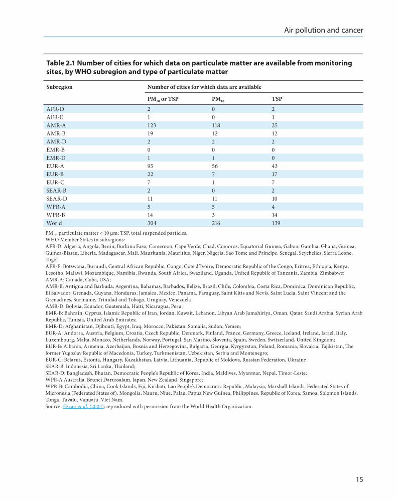
Table 2.1 shows the number of cities for which data on PM (measured as either total suspended particles or PM10) are available, by region of the world. It can be seen that the monitoring systems are much more widespread in North America and Europe.

Worldwide distribution of air pollutants

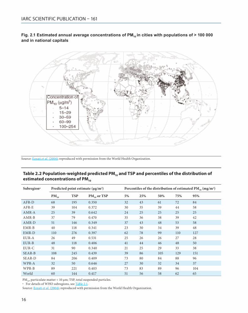
Fig. 2.1 shows the estimated annual average concentrations of PM10 in cities with populations > 100 000 and in national capitals. Table 2.2 gives the numbers represented in Fig. 2.1, which were estimated using the Global Model of Ambient Particulates (GMAPS) model developed by the World Bank (Cohen et al., 2004).

High concentrations of PM are observed in many parts of the world, with distinct clusters in South-East Asia, South America, and Africa. There is also wide variability in the estimated PM levels by WHO region. WHO Member States are grouped into six geographical regions: AFRO (Africa), AMRO (Americas), EMRO (Eastern Mediterranean), WHO Regional Office for Europe (Europe), SEARO (South-East Asia), and WPRO (Western Pacific). The highest concen-trations of PM (population-weighted) occur in parts of the WHO regions of AFRO (Algeria, Angola, Benin, Burkina Faso, Cameroon, Cape Verde, Chad, Comoros, Equatorial Guinea, Gabon, Gambia, Ghana, Guinea, Guinea-Bissau, Liberia, Madagascar, Mali, Mauritania, Mauritius, Niger, Nigeria, Sao Tome and Principe, Senegal, Seychelles, Sierra Leone, Togo), AMRO (Bolivia, Ecuador, Guatemala, Haiti, Nicaragua, Peru), SEARO (Bangladesh, Bhutan, Democratic People’s Republic of Korea, India, Indonesia, Maldives, Myanmar, Nepal, Sri Lanka, Thailand, Timor-Leste), and WPRO (Cambodia, China, Cook Islands, Fiji, Kiribati, Lao People’s Democratic Republic, Malaysia, Marshall Islands, Federated States of Micronesia, Mongolia, Nauru, Palau, Papua New Guinea, Philippines, Republic of Korea, Samoa, Solomon Islands, Tonga, Tuvalu, Vanuatu, Viet Nam). The six WHO regions are further divided, based on patterns of child and adult mortality, into subre-gions ranging from A (lowest) to E (highest).

Air pollution and cancer

15

Table 2 .1 Number of cities for which data on particulate matter are available from monitoring sites, by WHO subregion and type of particulate matter

Subregion Number of cities for which data are available

PM10 or TSP PM10 TSP

AFR-D 2 0 2AFR-E 1 0 1AMR-A 123 118 25AMR-B 19 12 12AMR-D 2 2 2EMR-B 0 0 0EMR-D 1 1 0EUR-A 95 56 43EUR-B 22 7 17EUR-C 7 1 7SEAR-B 2 0 2SEAR-D 11 11 10WPR-A 5 5 4WPR-B 14 3 14World 304 216 139PM10, particulate matter < 10 μm; TSP, total suspended particles.WHO Member States in subregions:AFR-D: Algeria, Angola, Benin, Burkina Faso, Cameroon, Cape Verde, Chad, Comoros, Equatorial Guinea, Gabon, Gambia, Ghana, Guinea, Guinea-Bissau, Liberia, Madagascar, Mali, Mauritania, Mauritius, Niger, Nigeria, Sao Tome and Principe, Senegal, Seychelles, Sierra Leone, Togo;AFR-E: Botswana, Burundi, Central African Republic, Congo, Côte d’Ivoire, Democratic Republic of the Congo, Eritrea, Ethiopia, Kenya, Lesotho, Malawi, Mozambique, Namibia, Rwanda, South Africa, Swaziland, Uganda, United Republic of Tanzania, Zambia, Zimbabwe;AMR-A: Canada, Cuba, USA;AMR-B: Antigua and Barbuda, Argentina, Bahamas, Barbados, Belize, Brazil, Chile, Colombia, Costa Rica, Dominica, Dominican Republic, El Salvador, Grenada, Guyana, Honduras, Jamaica, Mexico, Panama, Paraguay, Saint Kitts and Nevis, Saint Lucia, Saint Vincent and the Grenadines, Suriname, Trinidad and Tobago, Uruguay, VenezuelaAMR-D: Bolivia, Ecuador, Guatemala, Haiti, Nicaragua, Peru;EMR-B: Bahrain, Cyprus, Islamic Republic of Iran, Jordan, Kuwait, Lebanon, Libyan Arab Jamahiriya, Oman, Qatar, Saudi Arabia, Syrian Arab Republic, Tunisia, United Arab Emirates;EMR-D: Afghanistan, Djibouti, Egypt, Iraq, Morocco, Pakistan, Somalia, Sudan, Yemen;EUR-A: Andorra, Austria, Belgium, Croatia, Czech Republic, Denmark, Finland, France, Germany, Greece, Iceland, Ireland, Israel, Italy, Luxembourg, Malta, Monaco, Netherlands, Norway, Portugal, San Marino, Slovenia, Spain, Sweden, Switzerland, United Kingdom;EUR-B: Albania, Armenia, Azerbaijan, Bosnia and Herzegovina, Bulgaria, Georgia, Kyrgyzstan, Poland, Romania, Slovakia, Tajikistan, The former Yugoslav Republic of Macedonia, Turkey, Turkmenistan, Uzbekistan, Serbia and Montenegro;EUR-C: Belarus, Estonia, Hungary, Kazakhstan, Latvia, Lithuania, Republic of Moldova, Russian Federation, UkraineSEAR-B: Indonesia, Sri Lanka, Thailand;SEAR-D: Bangladesh, Bhutan, Democratic People’s Republic of Korea, India, Maldives, Myanmar, Nepal, Timor-Leste;WPR-A Australia, Brunei Darussalam, Japan, New Zealand, Singapore;WPR-B: Cambodia, China, Cook Islands, Fiji, Kiribati, Lao People’s Democratic Republic, Malaysia, Marshall Islands, Federated States of Micronesia (Federated States of), Mongolia, Nauru, Niue, Palau, Papua New Guinea, Philippines, Republic of Korea, Samoa, Solomon Islands, Tonga, Tuvalu, Vanuatu, Viet Nam.Source: Ezzati et al. (2004); reproduced with permission from the World Health Organization.

IARC SCIENTIFIC PUBLICATION – 161

16

Fig. 2.1 Estimated annual average concentrations of PM10 in cities with populations of > 100 000 and in national capitals

Source: Ezzati et al. (2004); reproduced with permission from the World Health Organization.

Table 2 .2 Population-weighted predicted PM10 and TSP and percentiles of the distribution of estimated concentrations of PM10

Subregiona Predicted point estimate (μg/m3) Percentiles of the distribution of estimated PM10 (mg/m3)

PM10 TSP PM10 or TSP 5% 25% 50% 75% 95%

AFR-D 68 195 0.350 32 43 61 72 84AFR-E 39 104 0.372 30 35 39 44 58AMR-A 25 39 0.642 24 25 25 25 25AMR-B 37 79 0.470 35 36 38 39 42AMR-D 51 146 0.349 37 43 48 53 58EMR-B 40 118 0.341 23 30 34 39 48EMR-D 110 276 0.397 62 78 99 110 127EUR-A 26 49 0.531 25 26 26 27 28EUR-B 48 118 0.406 41 44 46 48 50EUR-C 31 90 0.340 21 25 29 33 38SEAR-B 108 245 0.439 39 86 105 129 151SEAR-D 84 206 0.409 73 80 84 88 96WPR-A 32 50 0.646 27 30 32 34 37WPR-B 89 221 0.403 73 83 89 96 104World 60 144 0.417 51 56 58 62 65PM10, particulate matter < 10 μm; TSP, total suspended particles.a For details of WHO subregions, see Table 2.1.Source: Ezzati et al. (2004); reproduced with permission from the World Health Organization.

Air pollution and cancer

17

Distribution of pollutants in Europe

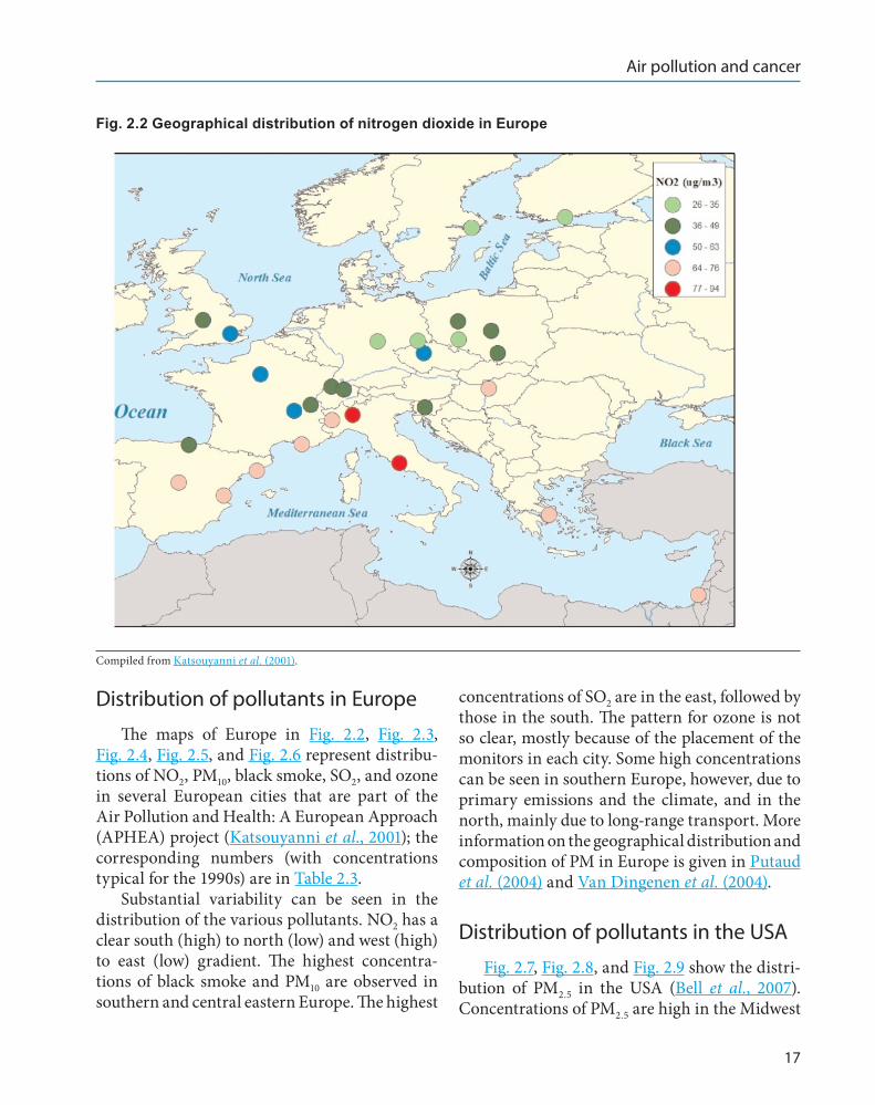
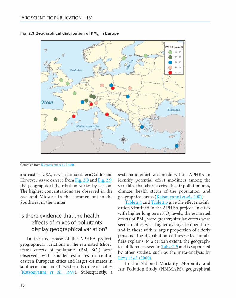
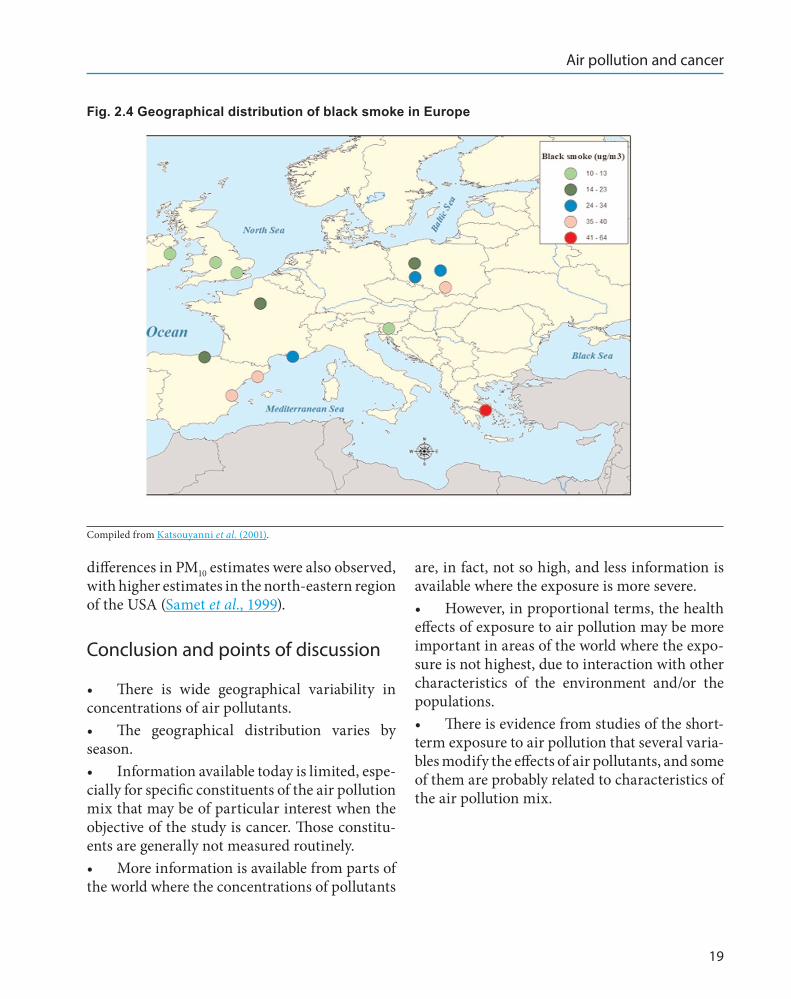
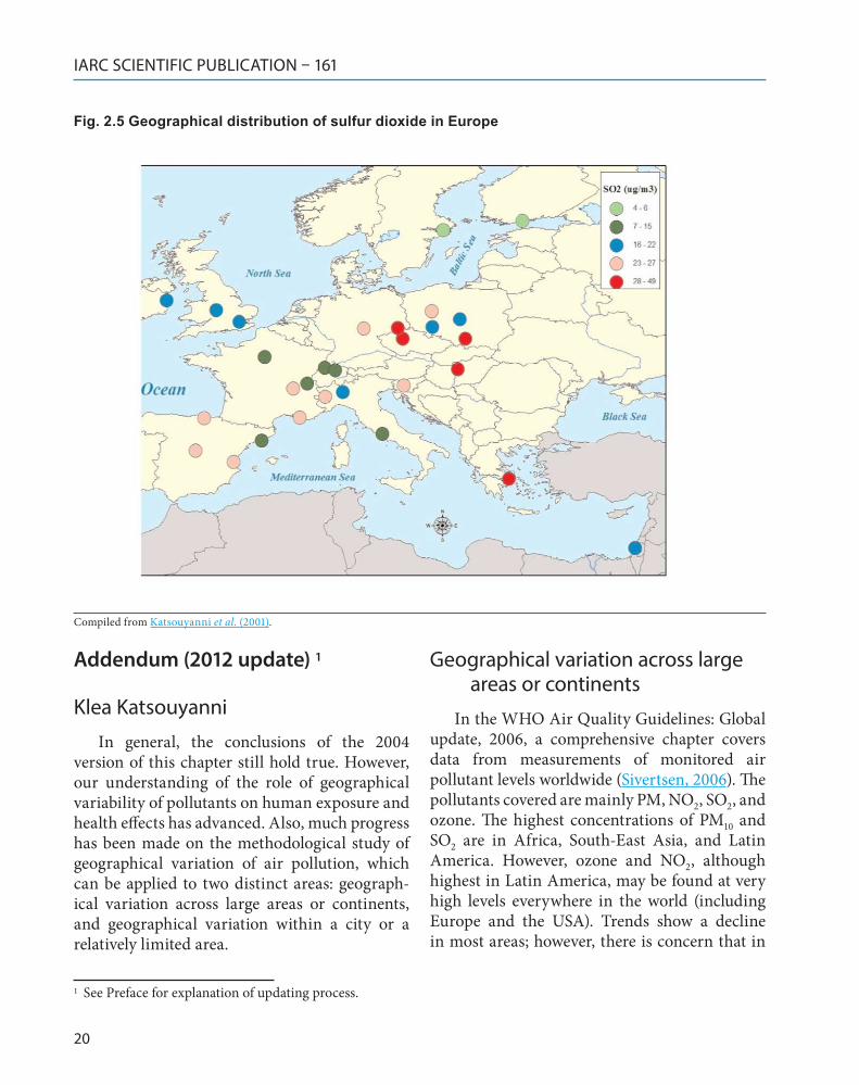
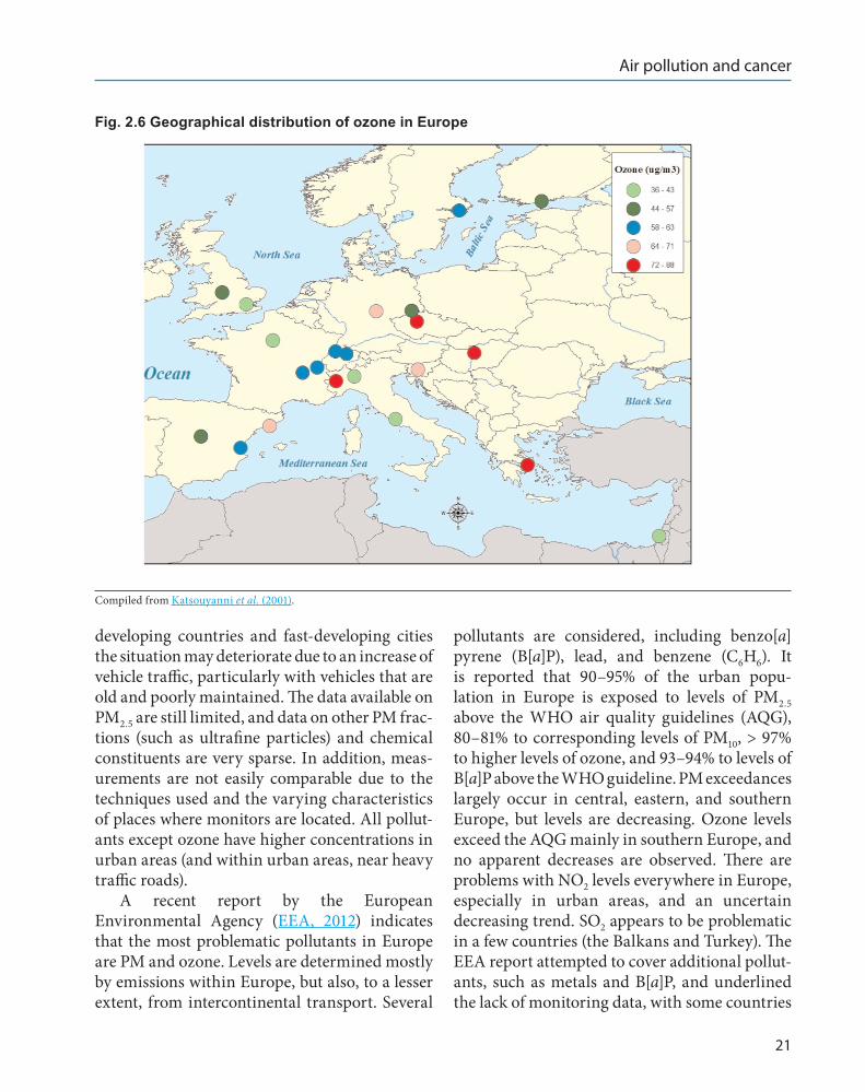
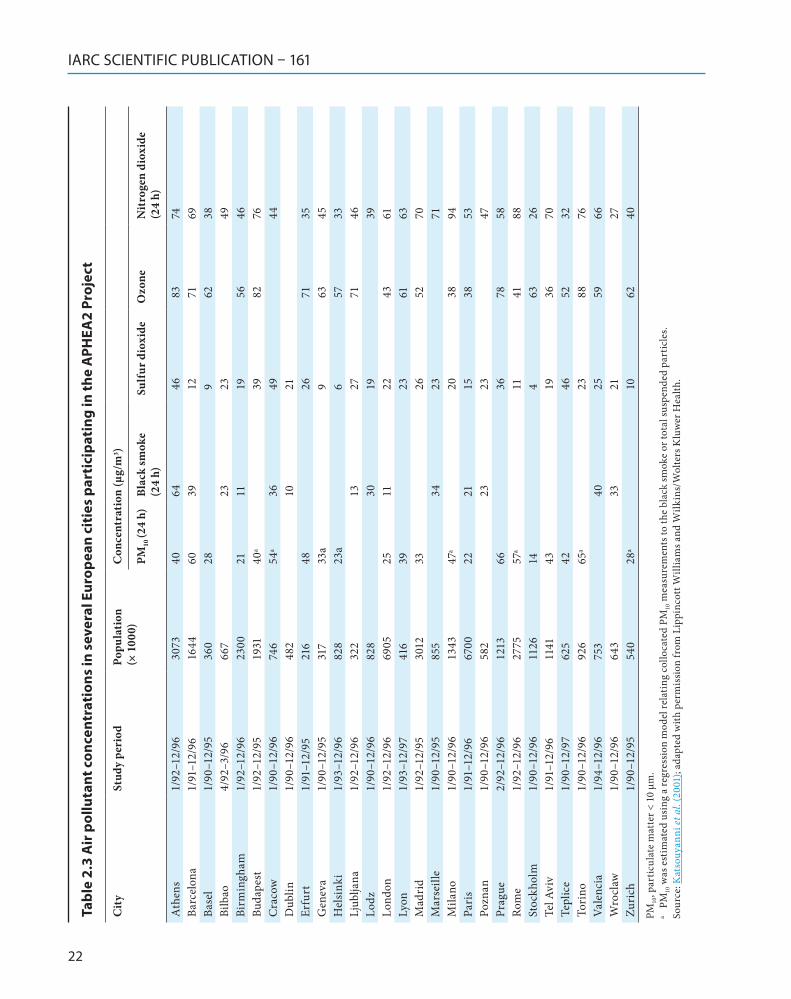
The maps of Europe in Fig.  2.2, Fig.  2.3, Fig. 2.4, Fig. 2.5, and Fig. 2.6 represent distribu-tions of NO2, PM10, black smoke, SO2, and ozone in several European cities that are part of the Air Pollution and Health: A European Approach (APHEA) project (Katsouyanni et al., 2001); the corresponding numbers (with concentrations typical for the 1990s) are in Table 2.3.

Substantial variability can be seen in the distribution of the various pollutants. NO2 has a clear south (high) to north (low) and west (high) to east (low) gradient. The highest concentra-tions of black smoke and PM10 are observed in southern and central eastern Europe. The highest

concentrations of SO2 are in the east, followed by those in the south. The pattern for ozone is not so clear, mostly because of the placement of the monitors in each city. Some high concentrations can be seen in southern Europe, however, due to primary emissions and the climate, and in the north, mainly due to long-range transport. More information on the geographical distribution and composition of PM in Europe is given in Putaud et al. (2004) and Van Dingenen et al. (2004).

Distribution of pollutants in the USA

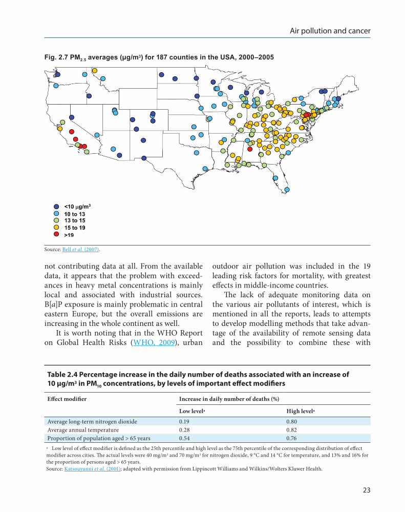
Fig. 2.7, Fig. 2.8, and Fig. 2.9 show the distri-bution of PM2.5 in the USA (Bell et al., 2007). Concentrations of PM2.5 are high in the Midwest

Fig. 2.2 Geographical distribution of nitrogen dioxide in Europe

 Compiled from Katsouyanni et al. (2001).

IARC SCIENTIFIC PUBLICATION – 161

18

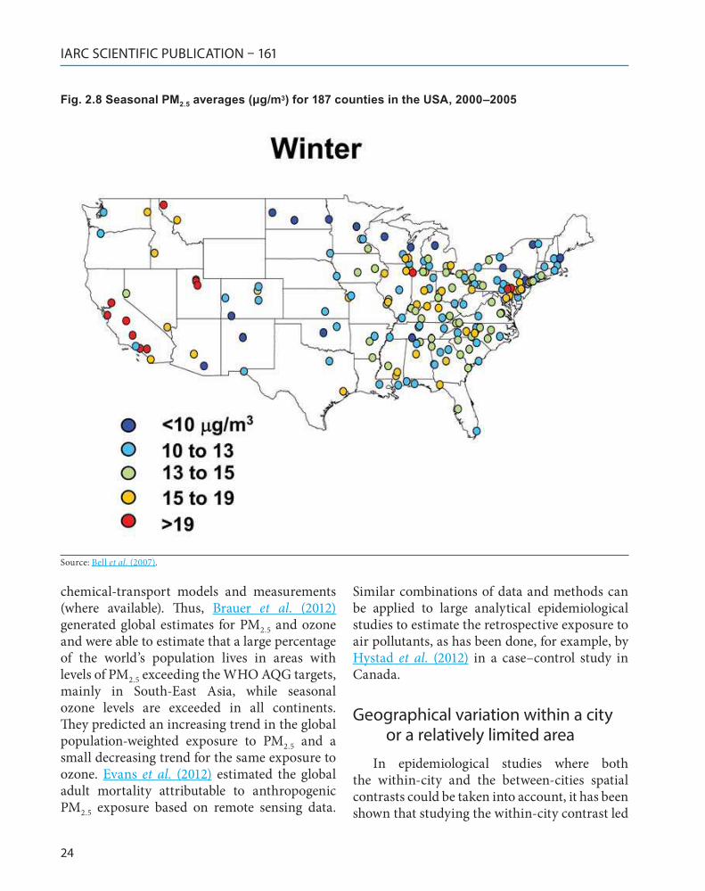
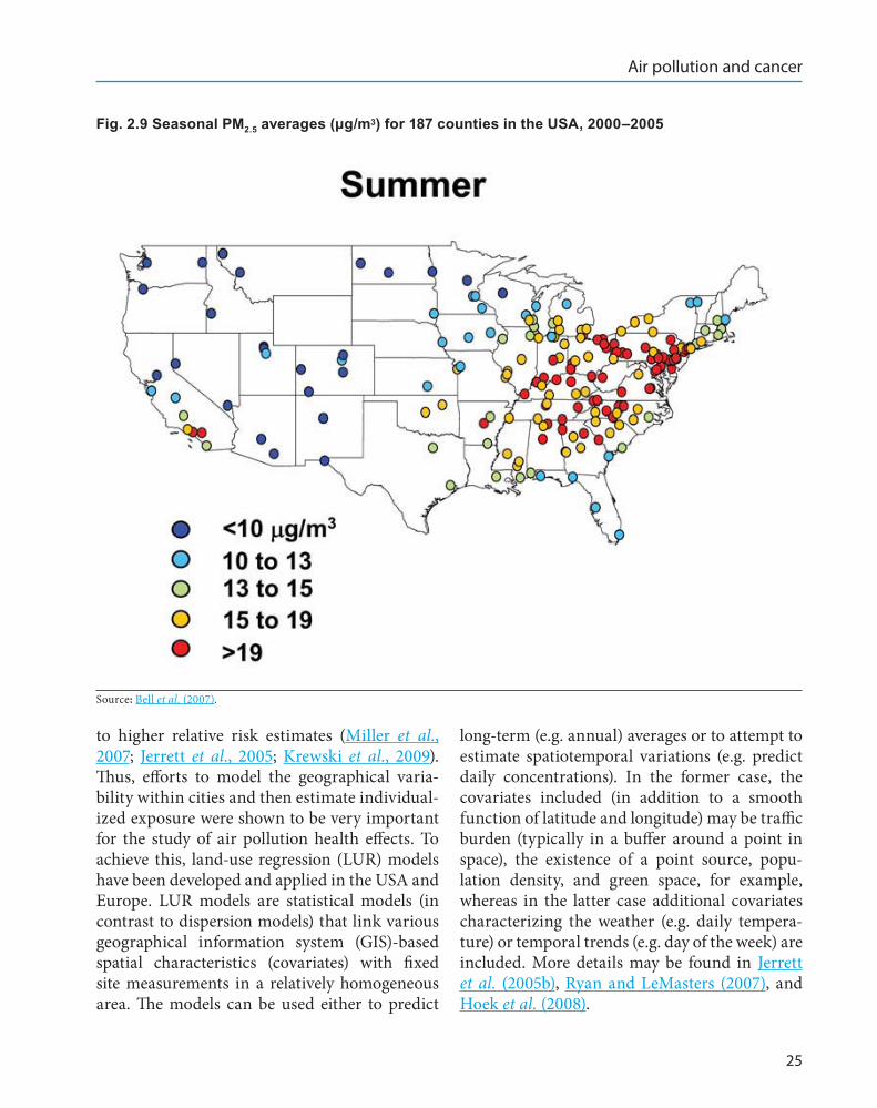
and eastern USA, as well as in southern California. However, as we can see from Fig. 2.8 and Fig. 2.9, the geographical distribution varies by season. The highest concentrations are observed in the east and Midwest in the summer, but in the Southwest in the winter.

Is there evidence that the health effects of mixes of pollutants display geographical variation?

In the first phase of the APHEA project, geographical variations in the estimated (short-term) effects of pollutants (PM, SO2) were observed, with smaller estimates in central eastern European cities and larger estimates in southern and north-western European cities (Katsouyanni et al., 1997). Subsequently, a

systematic effort was made within APHEA to identify potential effect modifiers among the variables that characterize the air pollution mix, climate, health status of the population, and geographical areas (Katsouyanni et al., 2001).

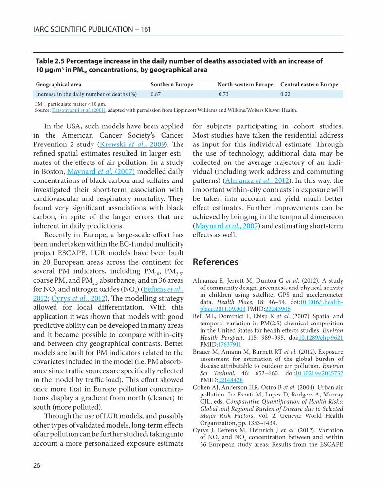
Table 2.4 and Table 2.5 give the effect modifi-cation identified in the APHEA project. In cities with higher long-term NO2 levels, the estimated effects of PM10 were greater; similar effects were seen in cities with higher average temperatures and in those with a larger proportion of elderly persons. The distribution of these effect modi-fiers explains, to a certain extent, the geograph-ical differences seen in Table 2.5 and is supported by other studies, such as the meta-analysis by Levy et al. (2000).

In the National Mortality, Morbidity and Air Pollution Study (NMMAPS), geographical

Fig. 2.3 Geographical distribution of PM10 in Europe

 

Compiled from Katsouyanni et al. (2001).

Air pollution and cancer

19

differences in PM10 estimates were also observed, with higher estimates in the north-eastern region of the USA (Samet et al., 1999).

Conclusion and points of discussion

• There is wide geographical variability in concentrations of air pollutants.• The geographical distribution varies by season.• Information available today is limited, espe-cially for specific constituents of the air pollution mix that may be of particular interest when the objective of the study is cancer. Those constitu-ents are generally not measured routinely.• More information is available from parts of the world where the concentrations of pollutants

are, in fact, not so high, and less information is available where the exposure is more severe.• However, in proportional terms, the health effects of exposure to air pollution may be more important in areas of the world where the expo-sure is not highest, due to interaction with other characteristics of the environment and/or the populations.• There is evidence from studies of the short-term exposure to air pollution that several varia-bles modify the effects of air pollutants, and some of them are probably related to characteristics of the air pollution mix.

Fig. 2.4 Geographical distribution of black smoke in Europe

 

Compiled from Katsouyanni et al. (2001).

IARC SCIENTIFIC PUBLICATION – 161

20

Addendum (2012 update) 1

Klea Katsouyanni

In general, the conclusions of the 2004 version of this chapter still hold true. However, our understanding of the role of geographical variability of pollutants on human exposure and health effects has advanced. Also, much progress has been made on the methodological study of geographical variation of air pollution, which can be applied to two distinct areas: geograph-ical variation across large areas or continents, and geographical variation within a city or a relatively limited area.

Geographical variation across large areas or continents

In the WHO Air Quality Guidelines: Global update, 2006, a comprehensive chapter covers data from measurements of monitored air pollutant levels worldwide (Sivertsen, 2006). The pollutants covered are mainly PM, NO2, SO2, and ozone. The highest concentrations of PM10 and SO2 are in Africa, South-East Asia, and Latin America. However, ozone and NO2, although highest in Latin America, may be found at very high levels everywhere in the world (including Europe and the USA). Trends show a decline in most areas; however, there is concern that in

1 See Preface for explanation of updating process.

Fig. 2.5 Geographical distribution of sulfur dioxide in Europe

Compiled from Katsouyanni et al. (2001).

Air pollution and cancer

21

developing countries and fast-developing cities the situation may deteriorate due to an increase of vehicle traffic, particularly with vehicles that are old and poorly maintained. The data available on PM2.5 are still limited, and data on other PM frac-tions (such as ultrafine particles) and chemical constituents are very sparse. In addition, meas-urements are not easily comparable due to the techniques used and the varying characteristics of places where monitors are located. All pollut-ants except ozone have higher concentrations in urban areas (and within urban areas, near heavy traffic roads).

A recent report by the European Environmental Agency (EEA, 2012) indicates that the most problematic pollutants in Europe are PM and ozone. Levels are determined mostly by emissions within Europe, but also, to a lesser extent, from intercontinental transport. Several

pollutants are considered, including benzo[a]pyrene (B[a]P), lead, and benzene (C6H6). It is reported that 90–95% of the urban popu-lation in Europe is exposed to levels of PM2.5 above the WHO air quality guidelines (AQG), 80–81% to corresponding levels of PM10, > 97% to higher levels of ozone, and 93–94% to levels of B[a]P above the WHO guideline. PM exceedances largely occur in central, eastern, and southern Europe, but levels are decreasing. Ozone levels exceed the AQG mainly in southern Europe, and no apparent decreases are observed. There are problems with NO2 levels everywhere in Europe, especially in urban areas, and an uncertain decreasing trend. SO2 appears to be problematic in a few countries (the Balkans and Turkey). The EEA report attempted to cover additional pollut-ants, such as metals and B[a]P, and underlined the lack of monitoring data, with some countries

Fig. 2.6 Geographical distribution of ozone in Europe

 

Compiled from Katsouyanni et al. (2001).

IARC SCIENTIFIC PUBLICATION – 161

22

Tabl

e 2 .

3 A

ir p

ollu

tant

con

cent

rati

ons

in s

ever

al E

urop

ean

citi

es p

arti

cipa

ting

in th

e A

PHEA

2 Pr

ojec

t

Cit

ySt

udy

peri

odPo

pula

tion

(×

 100

0)C

once

ntra

tion

(μg/

m3 )

PM10

(24 

h)Bl

ack

smok

e (2

4 h)

Sulf

ur d

ioxi

deO

zone

Nit

roge

n di

oxid

e (2

4 h)

Ath

ens

1/92

–12/

96  3

073

4064

  46

  83

74Ba

rcel

ona

1/91

–12/

96  1

644

6039

  12

  71

69Ba

sel

1/90

–12/

95  3

6028

  9  6

238

Bilb

ao4/

92–3

/96

  667

23  2

349

Birm

ingh

am1/

92–1

2/96

  230

021

11  1

9  5

646

Buda

pest

1/92

–12/

95  1

931

40a

  39

  82

76C

raco

w1/

90–1

2/96

  746

54a

36  4

944

Dub

lin1/

90–1

2/96

  482

10  2

1Er

furt

1/91

–12/

95  2

1648

  26

  71

35G

enev

a1/

90–1

2/95

  317

33a

  9  6

345

Hel

sink

i1/

93–1

2/96

  828

23a

  6  5

733

Ljub

ljana

1/92

–12/

96  3

2213

  27

  71

46Lo

dz1/

90–1

2/96

  828

30  1

939

Lond

on1/

92–1

2/96

  690

525

11  2

2  4

361

Lyon

1/93

–12/

97  4

1639

  23

  61

63M

adri

d1/

92–1

2/95

  301

233

  26

  52

70M

arse

ille

1/90

–12/

95  8

5534

  23

71M

ilano

1/90

–12/

96  1

343

47a

  20

  38

94Pa

ris

1/91

–12/

96  6

700

2221

  15

  38

53Po

znan

1/90

–12/

96  5

8223

  23

47Pr

ague

2/92

–12/

96  1

213

66  3

6  7

858

Rom

e1/

92–1

2/96

  277

557

a  1

1  4

188

Stoc

khol

m1/

90–1

2/96

  112

614

  4  6

326

Tel A

viv

1/91

–12/

96  1

141

43  1

9  3

670

Tepl

ice

1/90

–12/

97  6

2542

  46

  52

32To

rino

1/90

–12/

96  9

2665

a  2

3  8

876

Vale

ncia

1/94

–12/

96  7

5340

  25

  59

66W

rocl

aw1/

90–1

2/96

  643

33  2

127

Zuri

ch1/

90–1

2/95

  540

28a

  10

  62

40PM

10, p

artic

ulat

e m

atte

r < 1

0 μm

.a

PM

10 w

as e

stim

ated

usi

ng a

regr

essio

n m

odel

rela

ting

collo

cate

d PM

10 m

easu

rem

ents

to th

e bl

ack

smok

e or

tota

l sus

pend

ed p

artic

les.

Sour

ce: K

atso

uyan

ni et

al.

(200

1); a

dapt

ed w

ith p

erm

issio

n fr

om L

ippi

ncot

t Will

iam

s and

Wilk

ins/

Wol

ters

Klu

wer

Hea

lth.

Air pollution and cancer

23

not contributing data at all. From the available data, it appears that the problem with exceed-ances in heavy metal concentrations is mainly local and associated with industrial sources. B[a]P exposure is mainly problematic in central eastern Europe, but the overall emissions are increasing in the whole continent as well.

It is worth noting that in the WHO Report on Global Health Risks (WHO, 2009), urban

outdoor air pollution was included in the 19 leading risk factors for mortality, with greatest effects in middle-income countries.

The lack of adequate monitoring data on the various air pollutants of interest, which is mentioned in all the reports, leads to attempts to develop modelling methods that take advan-tage of the availability of remote sensing data and the possibility to combine these with

Fig. 2.7 PM2.5 averages (μg/m3) for 187 counties in the USA, 2000–2005

 

Source: Bell et al. (2007).

Table 2 .4 Percentage increase in the daily number of deaths associated with an increase of 10 µg/m3 in PM10 concentrations, by levels of important effect modifiers

Effect modifier Increase in daily number of deaths (%)

Low levela High levela

Average long-term nitrogen dioxide 0.19 0.80Average annual temperature 0.28 0.82Proportion of population aged > 65 years 0.54 0.76

a Low level of effect modifier is defined as the 25th percentile and high level as the 75th percentile of the corresponding distribution of effect modifier across cities. The actual levels were 40 mg/m3 and 70 mg/m3 for nitrogen dioxide, 9 °C and 14 °C for temperature, and 13% and 16% for the proportion of persons aged > 65 years.Source: Katsouyanni et al. (2001); adapted with permission from Lippincott Williams and Wilkins/Wolters Kluwer Health.

IARC SCIENTIFIC PUBLICATION – 161

24

chemical-transport models and measurements (where available). Thus, Brauer et al. (2012) generated global estimates for PM2.5 and ozone and were able to estimate that a large percentage of the world’s population lives in areas with levels of PM2.5 exceeding the WHO AQG targets, mainly in South-East Asia, while seasonal ozone levels are exceeded in all continents. They predicted an increasing trend in the global population-weighted exposure to PM2.5 and a small decreasing trend for the same exposure to ozone. Evans et al. (2012) estimated the global adult mortality attributable to anthropogenic PM2.5 exposure based on remote sensing data.

Similar combinations of data and methods can be applied to large analytical epidemiological studies to estimate the retrospective exposure to air pollutants, as has been done, for example, by Hystad et al. (2012) in a case–control study in Canada.

Geographical variation within a city or a relatively limited area

In epidemiological studies where both the within-city and the between-cities spatial contrasts could be taken into account, it has been shown that studying the within-city contrast led

Fig. 2.8 Seasonal PM2.5 averages (μg/m3) for 187 counties in the USA, 2000–2005

Source: Bell et al. (2007).

Air pollution and cancer

25

to higher relative risk estimates (Miller et al., 2007; Jerrett et al., 2005; Krewski et al., 2009). Thus, efforts to model the geographical varia-bility within cities and then estimate individual-ized exposure were shown to be very important for the study of air pollution health effects. To achieve this, land-use regression (LUR) models have been developed and applied in the USA and Europe. LUR models are statistical models (in contrast to dispersion models) that link various geographical information system (GIS)-based spatial characteristics (covariates) with fixed site measurements in a relatively homogeneous area. The models can be used either to predict

long-term (e.g. annual) averages or to attempt to estimate spatiotemporal variations (e.g. predict daily concentrations). In the former case, the covariates included (in addition to a smooth function of latitude and longitude) may be traffic burden (typically in a buffer around a point in space), the existence of a point source, popu-lation density, and green space, for example, whereas in the latter case additional covariates characterizing the weather (e.g. daily tempera-ture) or temporal trends (e.g. day of the week) are included. More details may be found in Jerrett et al. (2005b), Ryan and LeMasters (2007), and Hoek et al. (2008).

Fig. 2.9 Seasonal PM2.5 averages (μg/m3) for 187 counties in the USA, 2000–2005

 

Source: Bell et al. (2007).

IARC SCIENTIFIC PUBLICATION – 161

26

In the USA, such models have been applied in the American Cancer Society’s Cancer Prevention 2 study (Krewski et al., 2009). The refined spatial estimates resulted in larger esti-mates of the effects of air pollution. In a study in Boston, Maynard et al. (2007) modelled daily concentrations of black carbon and sulfates and investigated their short-term association with cardiovascular and respiratory mortality. They found very significant associations with black carbon, in spite of the larger errors that are inherent in daily predictions.

Recently in Europe, a large-scale effort has been undertaken within the EC-funded multicity project ESCAPE. LUR models have been built in 20 European areas across the continent for several PM indicators, including PM10, PM2.5, coarse PM, and PM2.5 absorbance, and in 36 areas for NO2 and nitrogen oxides (NOx) (Eeftens et al., 2012; Cyrys et al., 2012). The modelling strategy allowed for local differentiation. With this application it was shown that models with good predictive ability can be developed in many areas and it became possible to compare within-city and between-city geographical contrasts. Better models are built for PM indicators related to the covariates included in the model (i.e. PM absorb-ance since traffic sources are specifically reflected in the model by traffic load). This effort showed once more that in Europe pollution concentra-tions display a gradient from north (cleaner) to south (more polluted).

Through the use of LUR models, and possibly other types of validated models, long-term effects of air pollution can be further studied, taking into account a more personalized exposure estimate

for subjects participating in cohort studies. Most studies have taken the residential address as input for this individual estimate. Through the use of technology, additional data may be collected on the average trajectory of an indi-vidual (including work address and commuting patterns) (Almanza et al., 2012). In this way, the important within-city contrasts in exposure will be taken into account and yield much better effect estimates. Further improvements can be achieved by bringing in the temporal dimension (Maynard et al., 2007) and estimating short-term effects as well.

References

Almanza E, Jerrett M, Dunton G et  al. (2012). A study of community design, greenness, and physical activity in children using satellite, GPS and accelerometer data. Health Place, 18: 46–54. doi:10.1016/j.health-place.2011.09.003 PMID:22243906

Bell ML, Dominici F, Ebisu K et  al. (2007). Spatial and temporal variation in PM(2.5) chemical composition in the United States for health effects studies. Environ Health Perspect, 115: 989–995. doi:10.1289/ehp.9621 PMID:17637911

Brauer M, Amann M, Burnett RT et al. (2012). Exposure assessment for estimation of the global burden of disease attributable to outdoor air pollution. Environ Sci Technol, 46: 652–660. doi:10.1021/es2025752 PMID:22148428

Cohen AJ, Anderson HR, Ostro B et al. (2004). Urban air pollution. In: Ezzati M, Lopez D, Rodgers A, Murray CJL, eds. Comparative Quantification of Health Risks: Global and Regional Burden of Disease due to Selected Major Risk Factors, Vol. 2. Geneva: World Health Organization, pp. 1353–1434.

Cyrys J, Eeftens M, Heinrich J et  al. (2012). Variation of NO2 and NOx concentration between and within 36 European study areas: Results from the ESCAPE

Table 2 .5 Percentage increase in the daily number of deaths associated with an increase of 10 μg/m3 in PM10 concentrations, by geographical area

Geographical area Southern Europe North-western Europe Central eastern Europe

Increase in the daily number of deaths (%) 0.87 0.73 0.22PM10, particulate matter < 10 μm.Source: Katsouyanni et al. (2001); adapted with permission from Lippincott Williams and Wilkins/Wolters Kluwer Health.

Air pollution and cancer

27

study. Atmos Environ, 62: 374–390. doi:10.1016/j.atmosenv.2012.07.080

EEA (2012). Air Quality in Europe - 2012 Report, Copenhagen: European Environmental Agency.

Eeftens M, Beelen R, de Hoogh K et al. (2012). Development of Land Use Regression models for PM(2.5), PM(2.5) absorbance, PM(10) and PM(coarse) in 20 European study areas; results of the ESCAPE project. Environ Sci Technol, 46: 11195–11205. doi:10.1021/es301948k PMID:22963366

Evans J, van Donkelaar A, Martin RV et  al. (2012). Estimates of global mortality attributable to partic-ulate air pollution using satellite imagery. Environ Res, 120: 33–42. doi:10.1016/j.envres.2012.08.005 PMID:22959329

Ezzati M, Lopez AD, Rodgers A, Murray CJL (2004). Comparative Quantification of Health Risks: Global and Regional Burden of Disease due to Selected Major Risk Factors, Vol. 2. Geneva: World Health Organization. Available at http://whqlibdoc.who.int/publications/ 2004/9241580348_eng_Volume2.pdf

Hoek G, Beelen R, de Hoogh K et al. (2008). A review of land –use regression models to assess spatial variation of outdoor air pollution. Atmos Environ, 42: 7561–7578. doi:10.1016/j.atmosenv.2008.05.057

Hystad P, Demers PA, Johnson KC et  al. (2012). Spatiotemporal air pollution exposure assessment for a Canadian population-based lung cancer case-con-trol study. Environ Health, 11: 22 doi:10.1186/1476-069X-11-22 PMID:22475580

Jerrett M, Arain A, Kanaroglou P et al. (2005b). A review and evaluation of intraurban air pollution exposure models. J Expo Anal Environ Epidemiol, 15: 185–204. doi:10.1038/sj.jea.7500388 PMID:15292906

Jerrett M, Burnett RT, Ma R et al. (2005). Spatial analysis of air pollution and mortality in Los Angeles. Epidemiology, 16: 727–736. doi:10.1097/01.ede.0000181630.15826.7d PMID:16222161

Katsouyanni K, Touloumi G, Samoli E et  al. (2001). Confounding and effect modification in the short-term effects of ambient particles on total mortality: results from 29 European cities within the APHEA2 project. Epidemiology, 12: 521–531. doi:10.1097/00001648-200109000-00011 PMID:11505171

Katsouyanni K, Touloumi G, Spix C et al. (1997). Short-term effects of ambient sulphur dioxide and particulate matter on mortality in 12 European cities: results from time series data from the APHEA project. Air Pollution and Health: a European Approach. BMJ, 314: 1658–1663. doi:10.1136/bmj.314.7095.1658 PMID:9180068

Krewski D, Jerrett M, Burnett RT et al. (2009). Extended follow-up and spatial analysis of the American Cancer Society study linking particulate air pollution and mortality. Res Rep Health Eff Inst, 140: 5–114, discus-sion 115–136. PMID:19627030

Levy JI, Hammitt JK, Spengler JD (2000). Estimating the mortality impacts of particulate matter: what can be learned from between-study variability? Environ Health Perspect, 108: 109–117. doi:10.1289/ehp.00108109 PMID:10656850

Maynard D, Coull BA, Gryparis A, Schwartz J (2007). Mortality risk associated with short-term exposure to traffic particles and sulfates. Environ Health Perspect, 115: 751–755. doi:10.1289/ehp.9537 PMID:17520063

Miller KA, Siscovick DS, Sheppard L et al. (2007). Long-term exposure to air pollution and incidence of cardio-vascular events in women. N Engl J Med, 356: 447–458. doi:10.1056/NEJMoa054409 PMID:17267905

Putaud J, Raes FP, Van Dingenen RM et  al. (2004). A European aerosol phenomenology. Part 2: Chemical characteristics of particulate matter at kerbside, urban, rural and background sites in Europe. Atmos Environ, 38: 2579–2595. doi:10.1016/j.atmosenv.2004.01.041

Ryan PH & LeMasters GK (2007). A review of land-use regression models for characterizing intraurban air pollution exposure. Inhal Toxicol, 19: Suppl 1: 127–133. doi:10.1080/08958370701495998 PMID:17886060

Samet J, Zeger S, Dominici F et al. (1999). The National Mortality, Morbidity and Air Pollution Study (NMMAPS). Final Report. Boston, MA: Health Effects Institute (www.healtheffects.org)

Sivertsen B (2006). Global ambient air pollution concen-trations, trends. In: Air Quality Guidelines, Global Update 2005. Copenhagen: WHO Regional Office for Europe, pp. 31–59.

Van Dingenen RM, Raes FPE, Putaud J et  al. (2004). A European aerosol phenomenology. Part 1: Physical characteristics of particulate matter at kerbside, urban, rural and background sites in Europe. Atmos Environ, 38: 2561–2577. doi:10.1016/j.atmosenv.2004.01.040

WHO (2003). Health Aspects of Air Pollution with Particulate Matter, Ozone and Nitrogen Dioxide. Report on a WHO Working Group. EUR/03/5042688. Copenhagen: WHO Regional Office for Europe. Available at www.euro.who.int/document/e79097.pdf

WHO (2009). Global Health Risks: Mortality and Burden of Disease Attributable to Selected Major Risk Factors. Geneva: World Health Organization.