Chapter 21 Open Economy Macroeconomic Policy and Adjustment

Chapter 21

Open Economy Macroeconomic Policy and Adjustment

Copyright © 2007 Pearson Addison-Wesley. All rights reserved. 21-2

Topics to be Covered

• Internal Balance vs. External Balance

• Macroeconomic Equilibrium

• The IS Curve

• The LM Curve

• The BP Curve

• Monetary Policy and Fiscal Policy under Fixed Exchange Rates

• Monetary Policy and Fiscal Policy under Floating Exchange Rates


Topics to be Covered (cont.)

• The New Open Economy Macroeconomics

• International Policy Coordination

• The Open Economy Multiplier


Open Economy Goals: Internal and External Balance

• Internal Balance—a steady growth of the domestic economy consistent with a low unemployment rate.

• External Balance—the achievement of a desired trade balance or desired international capital flows.


Tools of Macroeconomic Policy

• Fiscal Policy—government spending and taxation.

• Monetary Policy—central bank control of the money supply and credit.


Macroeconomic Equilibrium

• Macroeconomic Equilibrium requires equilibrium in three major markets: Goods Market Equilibrium: the quantity of

goods and services supplied is equal to the quantity demanded.

Money Market Equilibrium: the quantity of money supplied is equal to the quantity demanded.

Balance of Payments Equilibrium: the current account deficit (surplus) is equal to the capital account surplus (deficit), so that the official settlements balance equals zero.


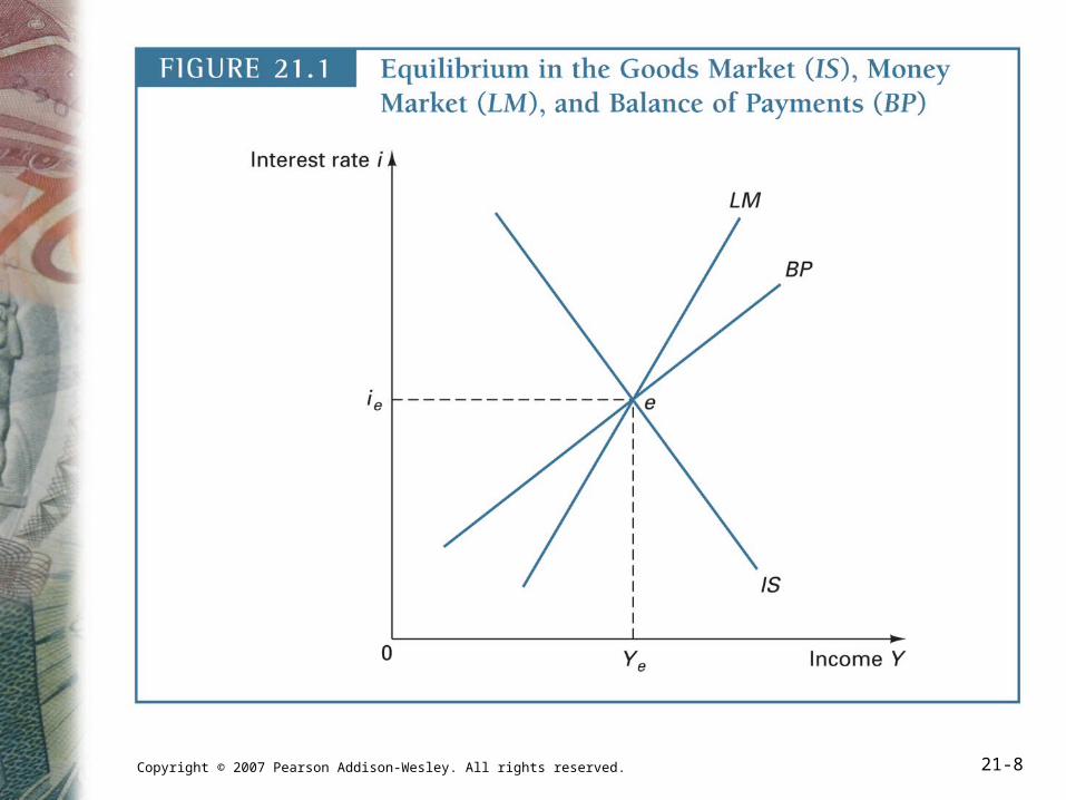
IS–LM–BP Model

• The IS curve represents the goods market equilibrium.

• The LM curve represents the money market equilibrium.

• The BP curve represents the balance of payments equilibrium.

• Macroeconomic equilibrium is achieved at the point where all the curves intersect.



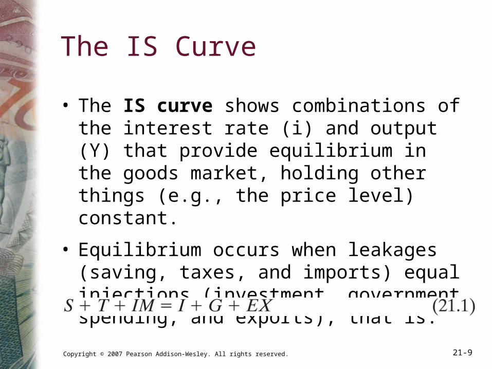
The IS Curve

• The IS curve shows combinations of the interest rate (i) and output (Y) that provide equilibrium in the goods market, holding other things (e.g., the price level) constant.

• Equilibrium occurs when leakages (saving, taxes, and imports) equal injections (investment, government spending, and exports), that is:


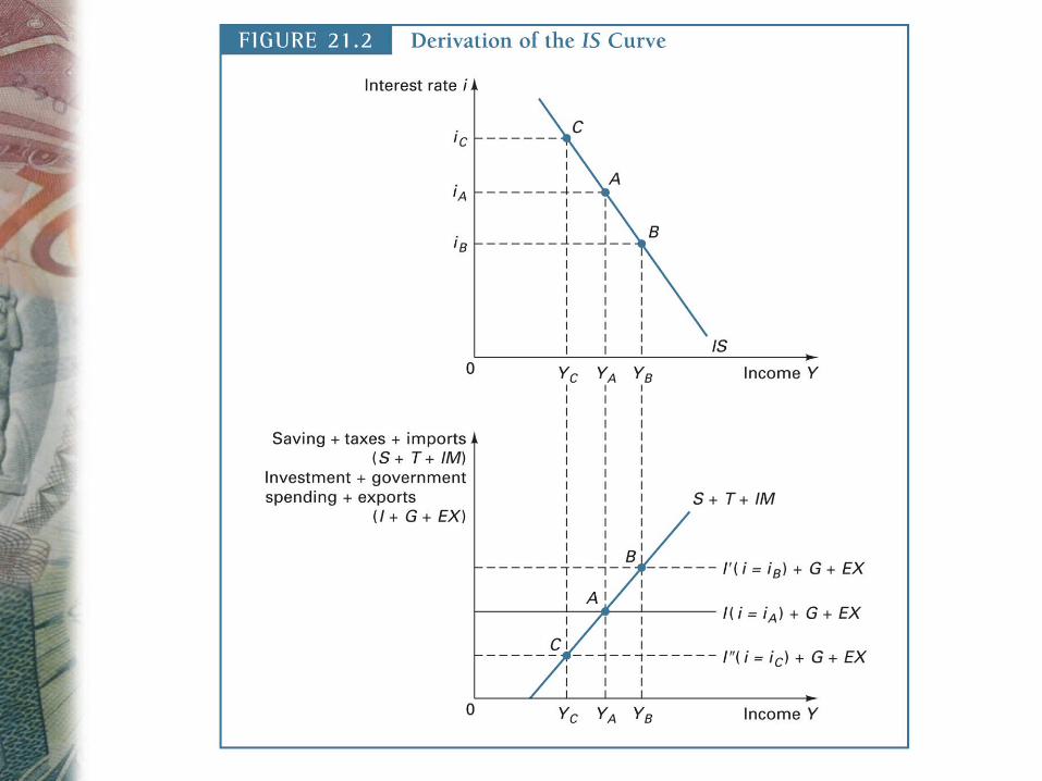
Deriving the IS Curve

• Refer to Figure 21.2 IS curve derivation

• Assumptions: S and IM depend positively on income T, I, G, and EX are independent of income I depends negatively on interest rate

• S + T + IM line is upward-sloping because as domestic income rises, S and IM increase.

• I + G + EX line is horizontal since I, G, and EX are independent of income.


Why is the IS Curve Downward-sloping?

• When the interest rate falls, more potential investment projects become profitable, and thus investment increases (I + G + EX line shifts upwards). As investment rises, equilibrium income also rises.


The LM Curve

• The LM curve shows combinations of i and Y that provide equilibrium in the money market.

• Graphically, money market equilibrium occurs at the intersection of the money supply curve and the money demand curve (refer to Figure 21.3).



Deriving the LM Curve

• Refer to Figure 21.3

• Assumptions: Money supply is determined by the central

bank and thus exogenous. Money demand is negatively related to i.

• Money supply curve is vertical.

• Money demand curve is downward-sloping.


Why is the LM Curve Upward-sloping?

• As income increases, demand for money would increase (money demand curve shifts upward). Given a fixed money supply, there will be an excess demand for money at the original interest rate. The desire to hold more money than is available will cause the interest rate to rise to a new equilibrium level.


The BP Curve

• The BP Curve shows combinations of i and Y that provide equilibrium in the balance of payments, holding the price level, exchange rate, and foreign debt constant.

• Graphically, equilibrium occurs at the intersection of the current account surplus line and the capital account deficit line (refer to Figure 21.4).


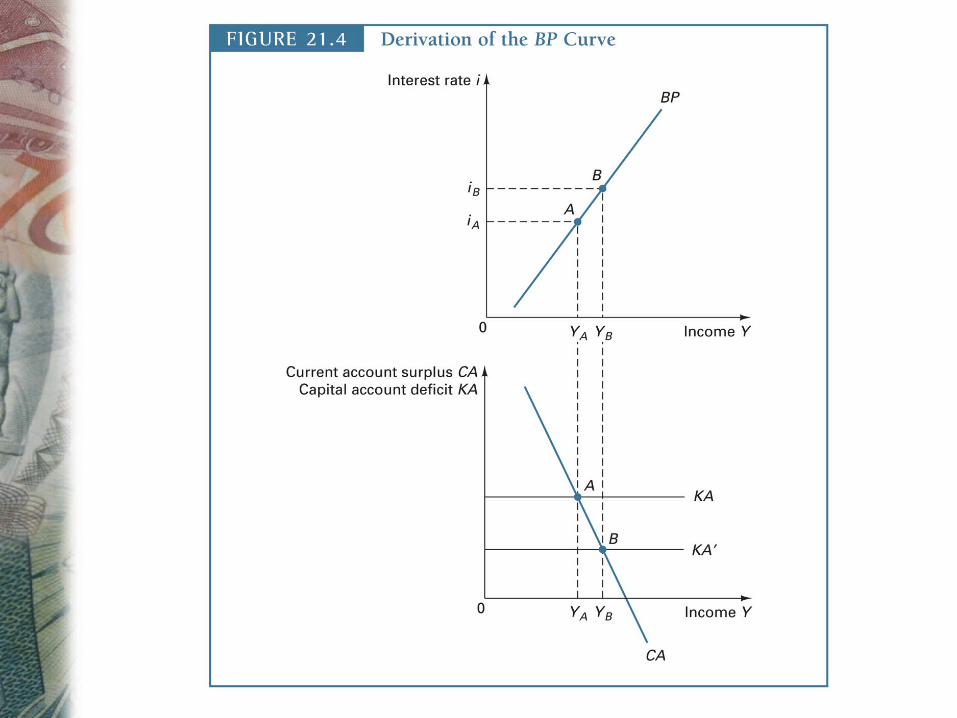
Deriving the BP Curve

• Refer to Figure 21.4

• The current account line is downward-sloping because as income increases, imports rise and the current account surplus falls.

• The capital account line is horizontal since the capital account is determined by i, not Y.


Why is the BP Curve Upward-sloping?

• If the interest rate increases, domestic financial assets become more attractive to foreign buyers, and the capital account deficit falls. At the old income level, the current account surplus will exceed the capital account deficit, so income must rise to a new equilibrium level.


Macroeconomic Equilibrium

• Equilibrium for the economy requires that all three markets (goods, money, and balance of payments) be in equilibrium.

• This occurs at the intersection point of the IS, LM, and BP curves.


IS–LM–BP Model with Fixed Exchange Rates

• Effects of Expansionary Monetary Policy

• Effects of Expansionary Fiscal Policy


Monetary Policy Under Fixed Exchange Rates

• With fixed exchange rates, the central bank is not free to conduct monetary policy independent of the rest of the world.

• Given perfect asset substitutability and perfect capital mobility, the domestic interest rate and foreign interest rate are equal, and the BP line is horizontal at i = iF. (refer to Figure 21.5)


Monetary Policy under Fixed XR (cont.)

• If the central bank increases the money supply, then the LM curves shifts to the right, resulting in a higher Y and lower i.

• The lower i causes a capital outflow and pressure on the domestic currency to depreciate.

• To maintain the fixed exchange rate, the central bank sells foreign exchange to buy domestic currency, thus reducing money supply and shifting the LM curve back to restore the initial equilibrium.

• Summary: Monetary policy is ineffective in changing Y under fixed exchange rates and perfect capital mobility.



Fiscal Policy Under Fixed Exchange Rates

• BP curve is horizontal at initial equilibrium interest rate (refer to Figure 21.6).

• An increase in government spending shifts the IS curve to the right, resulting in both higher i and Y.

• Higher i causes a capital inflow and pressure on the domestic currency to appreciate. The central bank must buy foreign exchange with domestic currency, thus increasing the money supply and shifting LM curve to the right. The new equilibrium is at the original interest rate but at a higher income level.

• Summary: Under fixed exchange rates, fiscal policy can increase income.



IS–LM–BP Model With Floating Exchange Rates

• The IS–LM–BP model with flexible exchange rates and perfect capital mobility is also called the Mundell-Fleming model.

• Effects of Expansionary Monetary Policy

• Effects of Expansionary Fiscal Policy


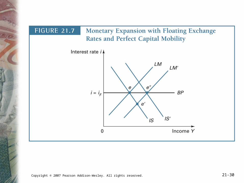
Monetary Policy Under Floating Exchange Rates

• With floating exchange rates, the domestic monetary policy is independent.

• Refer to Figure 21.7 An increase in money supply shifts LM to the right, resulting in a lower i and higher Y.

• The lower i causes a capital outflow and a depreciation of the domestic currency. The depreciation makes domestic goods relatively cheaper and stimulates net exports, thus shifting the IS curve to the right. The new equilibrium settles at the original i but at a higher income.

• Summary: Monetary policy can change income under floating exchange rates.



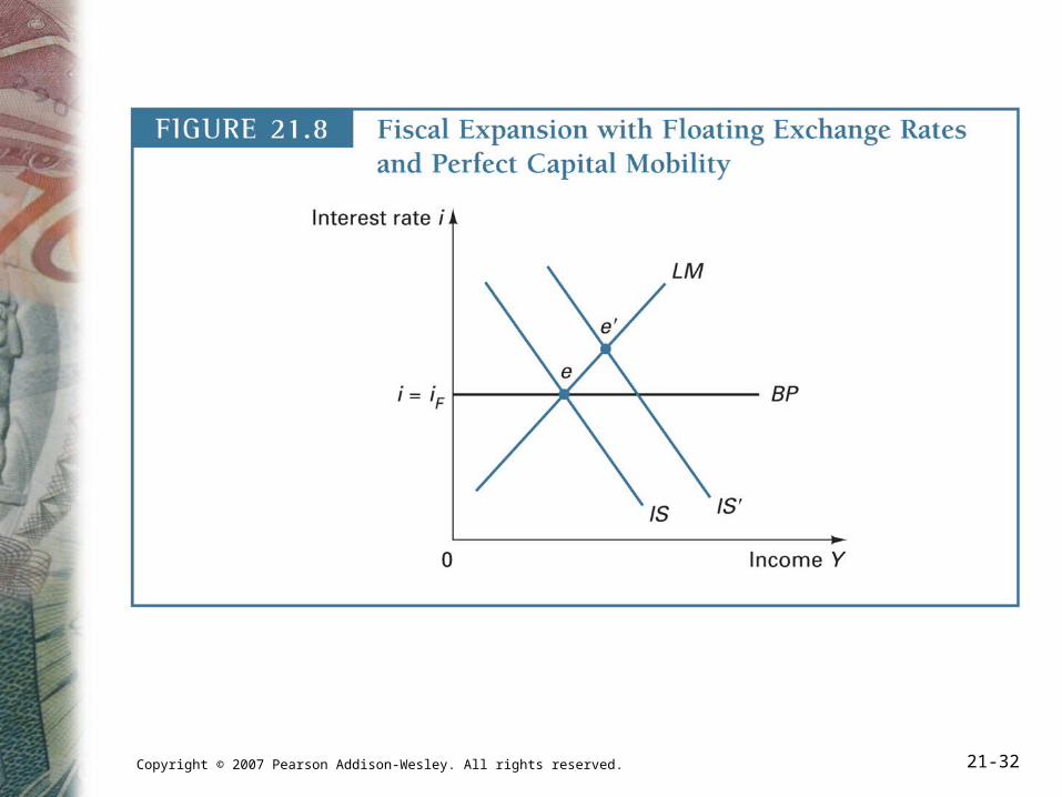
Fiscal Policy Under Floating Exchange Rates

• Refer to Figure 21.8• Expansionary fiscal policy shifts the IS curve

to the right resulting in both higher income and interest rate.

• The higher i attracts capital inflow, and the domestic currency appreciates. The appreciation shifts IS back to the original equilibrium i and Y.

• Summary: Fiscal policy is ineffective and there is complete crowding out, that is, the increase in government spending is offset by a decline in private spending.



The New Open Economy Macroeconomics

• The new macroeconomic models of open economies: Looks at households and firms and how their

actions aggregate to macroeconomic phenomena Examines two countries (or, one country and the

rest of the world) and the determination of macro variables such as income, prices, and the exchange rate

Assumes price level is fixed in short run but flexible in the long run

Allows for pricing to market behavior in which firms practice price discrimination across countries


International Policy Coordination

• If all countries coordinated their domestic policies: Crowding out could be minimized Exchange rates would be stabilized (although others

argue that exchange rates are determined by real economic shocks)

Beggar-thy-neighbor policies such as competitive devaluations could be avoided

A locomotive effect whereby a large country pulls other countries behind it may be produced

• The practical problem of policy coordination is the fact that different governments have different objectives.


The Open Economy Multiplier

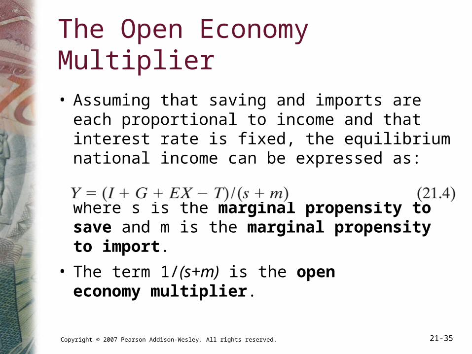
• Assuming that saving and imports are each proportional to income and that interest rate is fixed, the equilibrium national income can be expressed as:

where s is the marginal propensity to save and m is the marginal propensity to import.

• The term 1/(s+m) is the open economy multiplier.


Open Economy Multiplier (cont.)

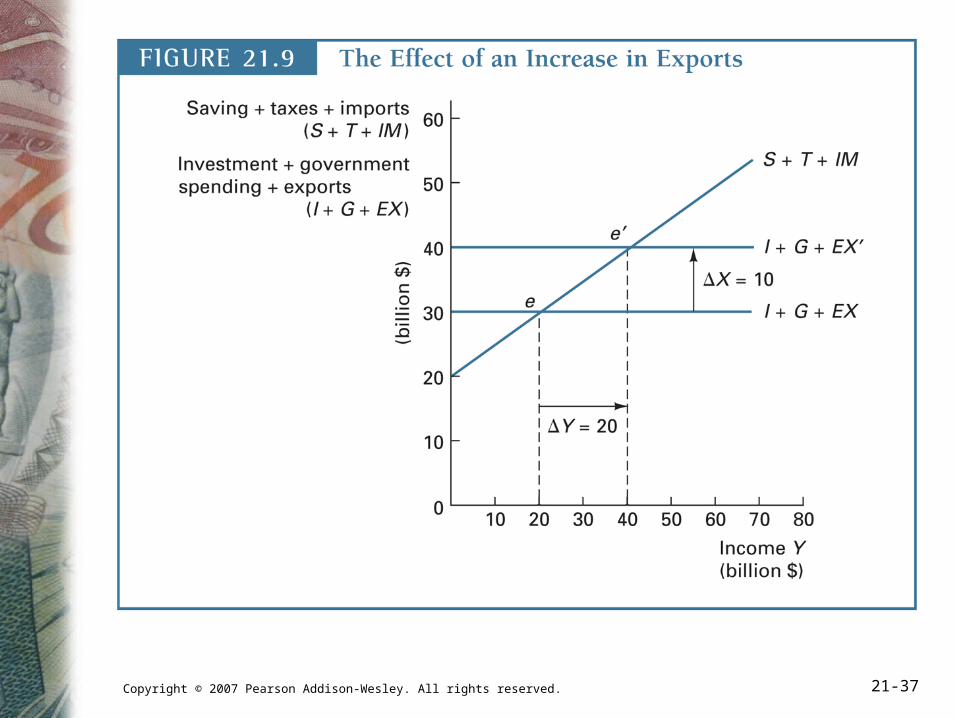
• Since s and m are fractions less than 1, then the multiplier is expected to be greater than 1. Thus, an increase in I, G, or EX would cause the equilibrium income level to rise by more than the change in spending.

• Refer to Figure 21.9 for example

• If exports increase, then the incomes of factors employed in the export industry will rise. These resource-owners (e.g., workers) will increase their spending on goods and services, thereby stimulating production, and further increases in income and spending (the multiplier effect).


Documents

Chapter 21 Open Economy Macroeconomic Policy and Adjustment