Chapter 3. Classical Demand Theory

(Part 1)Xiaoxiao Hu

October 18, 2021

3.A. Introduction: Take ! as the primitive

(1) Assumption(s) on ! so that ! can be represented with a

utility function

(2) Utility maximization and demand function

(3) Utility as a function of prices and wealth (indirect utility)

(4) Expenditure minimization and expenditure function

(5) Relationship among demand function, indirect utility func-

tion, and expenditure function2

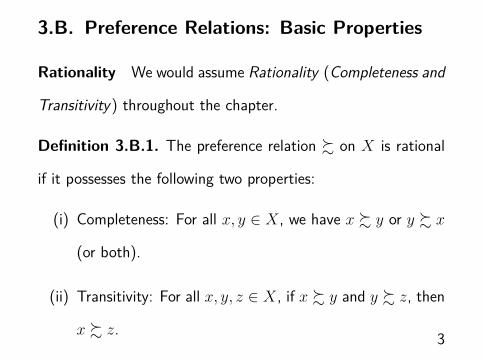
3.B. Preference Relations: Basic Properties

Rationality We would assume Rationality (Completeness and

Transitivity) throughout the chapter.

Definition 3.B.1. The preference relation ! on X is rational

if it possesses the following two properties:

(i) Completeness: For all x, y ∈ X, we have x ! y or y ! x

(or both).

(ii) Transitivity: For all x, y, z ∈ X, if x ! y and y ! z, then

x ! z. 3

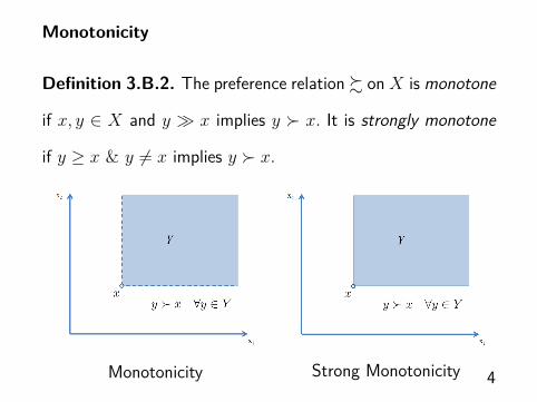
Monotonicity

Definition 3.B.2. The preference relation ! on X is monotone

if x, y ∈ X and y ≫ x implies y ≻ x. It is strongly monotone

if y ≥ x & y ∕= x implies y ≻ x.

Monotonicity Strong Monotonicity 4

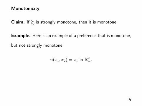
Monotonicity

Claim. If ! is strongly monotone, then it is monotone.

Example. Here is an example of a preference that is monotone,

but not strongly monotone:

u(x1, x2) = x1 in R2+.

5

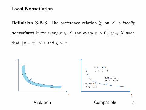
Local Nonsatiation

Definition 3.B.3. The preference relation ! on X is locally

nonsatiated if for every x ∈ X and every ε > 0, ∃y ∈ X such

that ‖y − x‖ ≤ ε and y ≻ x.

Violation Compatible 6

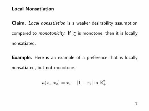
Local Nonsatiation

Claim. Local nonsatiation is a weaker desirability assumption

compared to monotonicity. If ! is monotone, then it is locally

nonsatiated.

Example. Here is an example of a preference that is locally

nonsatiated, but not monotone:

u(x1, x2) = x1 − |1 − x2| in R2+.

7

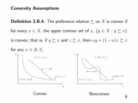
Convexity Assumptions

Definition 3.B.4. The preference relation ! on X is convex if

for every x ∈ X, the upper contour set of x, {y ∈ X : y ! x}

is convex; that is, if y ! x and z ! x, then αy + (1 − α)z ! x

for any α ∈ [0, 1].

Convex Nonconvex 8

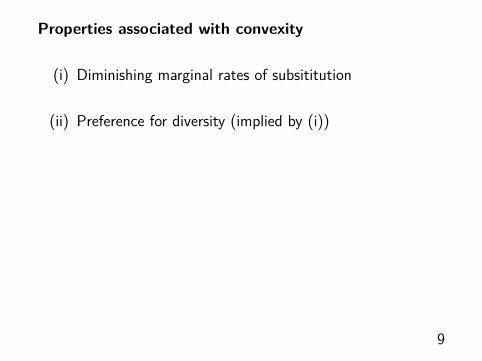
Properties associated with convexity

(i) Diminishing marginal rates of subsititution

(ii) Preference for diversity (implied by (i))

9

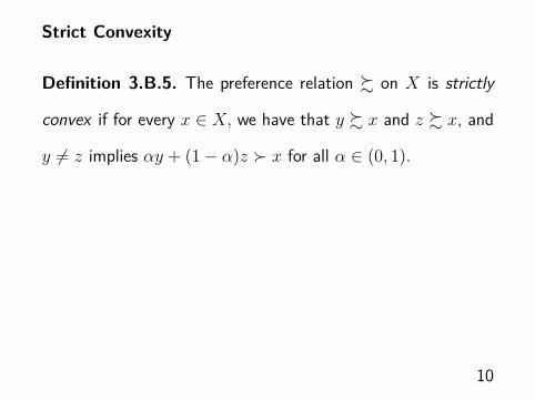
Strict Convexity

Definition 3.B.5. The preference relation ! on X is strictly

convex if for every x ∈ X, we have that y ! x and z ! x, and

y ∕= z implies αy + (1 − α)z ≻ x for all α ∈ (0, 1).

10

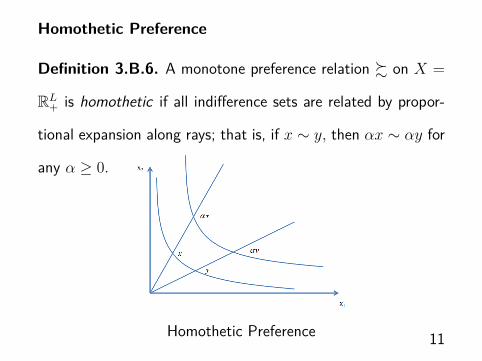
Homothetic Preference

Definition 3.B.6. A monotone preference relation ! on X =

RL+ is homothetic if all indifference sets are related by propor-

tional expansion along rays; that is, if x ∼ y, then αx ∼ αy for

any α ≥ 0.

Homothetic Preference 11

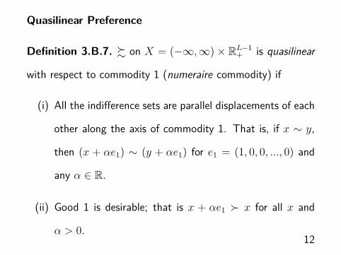
Quasilinear Preference

Definition 3.B.7. ! on X = (−∞, ∞) × RL−1+ is quasilinear

with respect to commodity 1 (numeraire commodity) if

(i) All the indifference sets are parallel displacements of each

other along the axis of commodity 1. That is, if x ∼ y,

then (x + αe1) ∼ (y + αe1) for e1 = (1, 0, 0, ..., 0) and

any α ∈ R.

(ii) Good 1 is desirable; that is x + αe1 ≻ x for all x and

α > 0.12

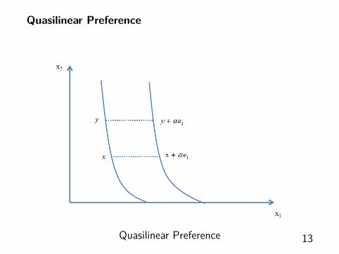
Quasilinear Preference

Quasilinear Preference 13

3.C. Preference and Utility

Key Question. When can a rational preference relation be

represented by a utility function?

Answer: If the preference relation is continuous.

14

Continuous Preference

Definition 3.C.1. The preference relation ! on X is contin-

uous if it is preserved in the limits. That is, for any sequence

of pairs {(xn, yn)}∞n=1 with xn ! yn for all n, x = lim

n→∞xn,

y = limn→∞

yn, we have x ! y.

15

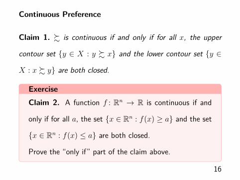
Continuous Preference

Claim 1. ! is continuous if and only if for all x, the upper

contour set {y ∈ X : y ! x} and the lower contour set {y ∈

X : x ! y} are both closed.

ExerciseClaim 2. A function f : Rn → R is continuous if and

only if for all a, the set {x ∈ Rn : f(x) ≥ a} and the set

{x ∈ Rn : f(x) ≤ a} are both closed.

Prove the “only if” part of the claim above.

16

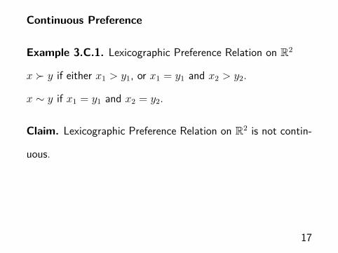
Continuous Preference

Example 3.C.1. Lexicographic Preference Relation on R2

x ≻ y if either x1 > y1, or x1 = y1 and x2 > y2.

x ∼ y if x1 = y1 and x2 = y2.

Claim. Lexicographic Preference Relation on R2 is not contin-

uous.

17

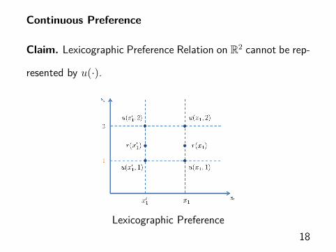
Continuous Preference

Claim. Lexicographic Preference Relation on R2 cannot be rep-

resented by u(·).

Lexicographic Preference18

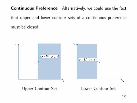
Continuous Preference Alternatively, we could use the fact

that upper and lower contour sets of a continuous preference

must be closed.

Upper Contour Set Lower Contour Set

19

Continuous Preference

Proposition 3.C.1 (Debreu’s theorem). Suppose that the pref-

erence relation! on X is continuous and monotone. Then there

exists continuous utility function u(x) that represents !, i.e.,

u(x) ≥ u(y) if and only if x ! y.

20

Continuous Preference

Remark. u(x) is not unique, any increasing transformation v(x) =

f(u(x)) will represent !. We can also introduce countably

many jumps in f(·).

21

Assumptions of differentiability of u(x)

The assumption of differentiability is commonly adopted for

technical convenience, but is not applicable to all useful models.

22

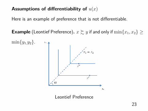
Assumptions of differentiability of u(x)

Here is an example of preference that is not differentiable.

Example (Leontief Preference). x ! y if and only if min{x1, x2} ≥

min{y1,y2}.

Leontief Preference23

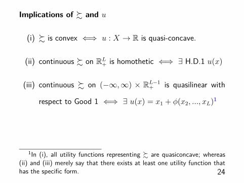
Implications of ! and u

(i) ! is convex ⇐⇒ u : X → R is quasi-concave.

(ii) continuous ! on RL+ is homothetic ⇐⇒ ∃ H.D.1 u(x)

(iii) continuous ! on (−∞, ∞) × RL−1+ is quasilinear with

respect to Good 1 ⇐⇒ ∃ u(x) = x1 + φ(x2, ..., xL)1

1In (i), all utility functions representing ! are quasiconcave; whereas(ii) and (iii) merely say that there exists at least one utility function thathas the specific form. 24

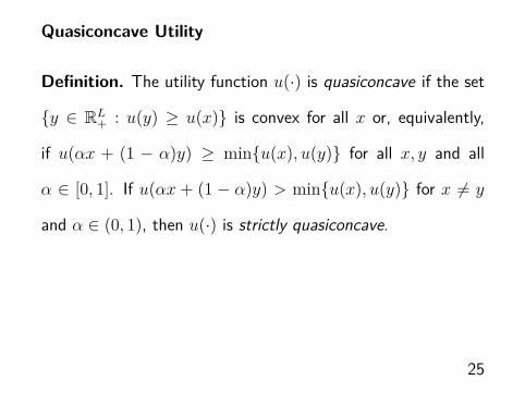
Quasiconcave Utility

Definition. The utility function u(·) is quasiconcave if the set

{y ∈ RL+ : u(y) ≥ u(x)} is convex for all x or, equivalently,

if u(αx + (1 − α)y) ≥ min{u(x), u(y)} for all x, y and all

α ∈ [0, 1]. If u(αx + (1 − α)y) > min{u(x), u(y)} for x ∕= y

and α ∈ (0, 1), then u(·) is strictly quasiconcave.

25

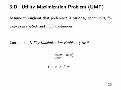
3.D. Utility Maximization Problem (UMP)

Assume throughout that preference is rational, continuous, lo-

cally nonsatiated, and u(x) continuous.

Consumer’s Utility Maximization Problem (UMP):

maxx∈RL

+

u(x)

s.t. p · x ≤ w

26

Existence of Solution

Proposition 3.D.1. If p ≫ 0 and u(·) is continuous, then the

utility maximization problem has a solution.

27

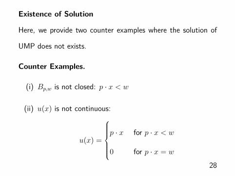
Existence of Solution

Here, we provide two counter examples where the solution of

UMP does not exists.

Counter Examples.

(i) Bp,w is not closed: p · x < w

(ii) u(x) is not continuous:

u(x) =

!""""#

""""$

p · x for p · x < w

0 for p · x = w

28

Walrasian demand correspondence/functions

The solution of UMP, denoted by x(p, w), is called Walrasian

(or ordinary or market) demand correspondence.

When x(p, w) is single valued for all (p, w), we refer to it as

Walrasian (or ordinary or market) demand function.

29

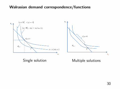
Walrasian demand correspondence/functions

Single solution Multiple solutions

30

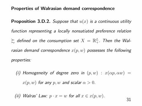
Properties of Walrasian demand correspondence

Proposition 3.D.2. Suppose that u(x) is a continuous utility

function representing a locally nonsatiated preference relation

! defined on the consumption set X = RL+. Then the Wal-

rasian demand correspondence x(p, w) possesses the following

properties:

(i) Homogeneity of degree zero in (p, w) : x(αp, αw) =

x(p, w) for any p, w and scalar α > 0.

(ii) Walras’ Law: p · x = w for all x ∈ x(p, w).31

Properties of Walrasian demand correspondence

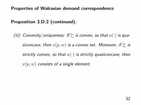
Proposition 3.D.2 (continued).

(iii) Convexity/uniqueness: If ! is convex, so that u(·) is qua-

siconcave, then x(p, w) is a convex set. Moreover, if ! is

strictly convex, so that u(·) is strictly quasiconcave, then

x(p, w) consists of a single element.

32

We will take a break to review some mathematical results before

proceeding with this Chapter.

33