40

CHAPTER 3

GENETIC ALGORITHM BASED PI

CONTROLLER TUNING

3.1 INTRODUCTION

Over the years, control of process system plants in the industry is

customarily carried out by experts through the conventional PID control

techniques. This is due to its simplicity, low cost design and robust

performance in a wide range of operating conditions. According to an

estimate, nearly 90% of the controllers used in industries are PID controllers.

The family of PID controllers is rigidly known as the building blocks of

control systems owing to their simplicity and ease of implementation.

Although the PID controllers have gained widespread usage across

technological industries, it must also be pointed out that the unnecessary

mathematical rigor, preciseness and accuracy involved with the design of the

controllers have been a major drawback. Designing and tuning a PID

controller appears to be conceptually intuitive, but can be hard in practice, if

multiple objectives are to be achieved (Huailin Shu and Youguo Pi 2005).

However various techniques and modifications to the conventional PID

controllers have been employed in order to overcome these difficulties. This

includes the use of auto tuning PID controllers, adaptive PID controllers and

also the implementation of compensation schemes to the PID controllers.

41

But as a whole the PID controllers are with some drawbacks of

design of the controllers for electric drives. In simple PID controllers it is

difficult to generate a derivative term in the output that has any significant

effect on motor speed. It can be deployed to reduce the rapid speed oscillation

caused by high proportional gain. However in many controllers, it is not used.

The derivative action causes the noise (random error) in the main signal to be

amplified and reflected in the controller output. Hence the most suitable

controller for speed control is PI type controller. Here, a PI type controller is

used to correct the motor speed. The proportional term does the job of fast

acting correction which will produce a change in the output as quickly as the

error arises. The integral action takes a finite time to act but has the capability

to make the steady state speed error zero.

Genetic Algorithm which is adopted from the biological evaluation,

is an efficient search technique that manipulates the coding representing a

parameter set to search a near optimal solution through cooperation and

competition among the potential solutions (Ravi and Balakrishnan 2011).

This algorithm is highly relevant for industrial applications, because it is

capable of handling problems with nonlinear constraints, multiple objectives

and dynamic components. Genetic Algorithm is composed of two main

elements which are strongly related to the problems being solved by the

encoding scheme and the evaluation function. The encoding scheme is used to

represent the possible solutions to the problem. Individual parameters can be

encoded in some alphabets like binary strings, real numbers and vectors.

While applying Genetic Algorithm practically, a population pool of

chromosomes is installed and it is set to a random value. In each cycle of

genetic evaluation, a subsequent generation is created from the chromosomes

in the current population. The cycle of evaluation is repeated until a

termination criterion is reached. Fitness value can be set as the termination

criterion.

42

3.2 PI CONTROL ALGORITHM

A proportional-Integral (PI) controller is a generic control loop

feedback mechanism (controller) widely used in industrial control systems . A

PI is the most commonly used controller and it calculates an "error" value as

the difference between a measured process variable and a desired set point.

The controller attempts to minimize the error by adjusting the process control

inputs. The Proportional and Integral values are denoted as P and I.

Heuristically, these values can be interpreted in terms of time such as

P depends on the present error and I depends on the accumulation of past

errors. The weighted sum of these two actions is used to adjust the process via

a control element such as the position of a control valve, or the power

supplied to a heating element.

By tuning the two parameters in the PI controller algorithm, the

controller can provide control action designed for specific process

requirements. The response of the controller can be described in terms of the

responsiveness of the controller to an error, the degree to which the

controller overshoots the set point and the degree of system oscillation. Some

applications may require using only one or two actions to provide the

appropriate system control. This is achieved by setting the other parameters to

zero. A PI controller will be called a P or I controller in the absence of the

other parameter.

According to the system requirements, the PI controller is designed.

PI controller consists of two types of controls namely Proportional and

Integral control and is shown in Figure 3.1. The transfer function of the PI

controller for continuous system is defined as follows.

sKKsG i

pc )( (3.1)

43

The transfer function of the PI controller for discrete system is

defined as follows.

)

1()(

zzTKKzG ipc (3.2)

where,

Kp = the proportional gain constant

Ki = the integral gain constant

Figure 3.1 Block diagram of system with PI Controller

First, let's take a look at the effect of a PI controller on the closed

loop system using the schematic above. To begin with, variable ‘e’ is the

tracking error or the difference between the desired reference value and the

actual output. The controller takes this error signal and computes both its

proportional and its integral values. The signal which is sent to the actuator is

now equal to the proportional gain (Kp) times the magnitude of the error plus

the integral gain (Ki) times the integral of the error . As the name suggests,

the PI algorithm consists of two basic modes namely the Proportional mode

and the Integral mode. When utilizing this algorithm it is necessary to decide

the modes that are to be used and then specify the parameters for each mode

44

used. Two basic algorithms used are P or PI. Tuning a system means

adjusting two parameters Kp and Ki adding various amounts of these

parameters to get the system to behave in the desired manner. Although it is

found many methods and theories on tuning a PI, there is a straight forward

approach to get you up and solving quickly.

1. SET Kp. Starting with Kp=0 and Ki=0, increase Kp until the

output starts overshooting and reducing the settling time

significantly.

2. SET Ki. Increase Ki until the final error is equal to zero.

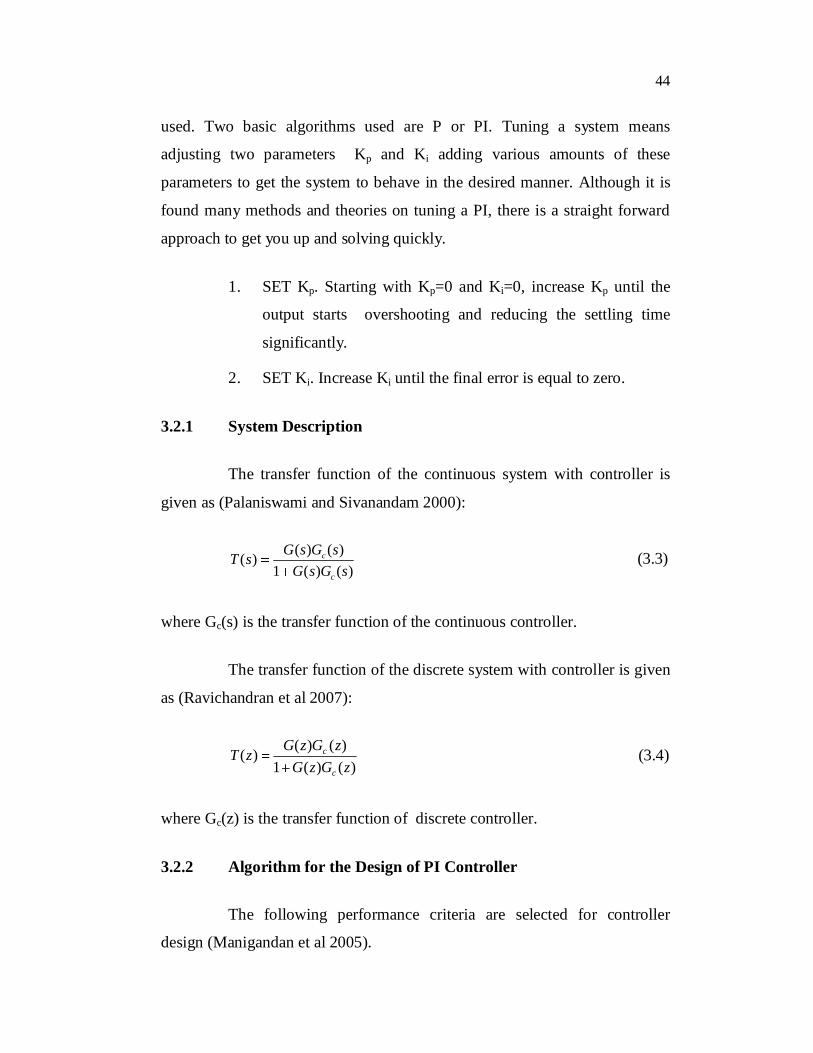
3.2.1 System Description

The transfer function of the continuous system with controller is

given as (Palaniswami and Sivanandam 2000):

)()(1

)()()(sGsG

sGsGsTc

c (3.3)

where Gc(s) is the transfer function of the continuous controller.

The transfer function of the discrete system with controller is given

as (Ravichandran et al 2007):

)()(1)()()(zGzG

zGzGzTc

c (3.4)

where Gc(z) is the transfer function of discrete controller.

3.2.2 Algorithm for the Design of PI Controller

The following performance criteria are selected for controller

design (Manigandan et al 2005).

45

Settling time 3 seconds

Peak overshoot 2%

Steady state error 1%

The following steps are considered for the design of PI controller.

Read the open loop transfer function of the given higher order

system.

Form the closed loop transfer function.

Obtain the step response of closed loop system.

Check the response for the required specifications.

If the specifications are not met, get a reduced order

model and design a controller for the reduced order model.

Obtain the initial values of the parameter Kp and Ki by pole

zero Cancellation method.

Cascade the controller with reduced order model and get the

closed loop response with the initial values of the controller

parameters.

Find the optimum values for the controller parameters which

satisfy the required specifications.

By applying the optimum values, cascade this controller with

the original system.

Obtain the closed loop step response of the system with the

controller.

46

If the specifications are met give exit command else tune the

parameters of the controller till they meet the required

specifications.

For designing the PI controller, the values of controller parameters

Kp and Ki are obtained through existing tuning method. The GA is

employed to obtain the optimized values of Kp and Ki to meet out the

designs specifications.

3.3 EXISTING TUNING METHODS

The existing tuning methods that are mainly used to control motor

drives include,

Ziegler-Nichols (Z-N) method

Magnitude Optimum (MO) method

Symmetric Optimum (SO) tuning method

3.3.1 Ziegler–Nichols Tuning Method

A very useful empirical formula was proposed by Ziegler and

Nichols in early 1942 (Ziegler and Nichols 1942). The tuning formula is

obtained when the plant model is given by a first order plus dead time

(FOPDT) which can be expressed by

sLe

sTksG

1)( (3.5)

In real time process control systems, a large variety of plants can be

approximately modeled according to Equation (3.5). If the system model

cannot be physically derived, experiments can be performed to extract the

parameters for the approximate model (3.5). For instance, if the step response

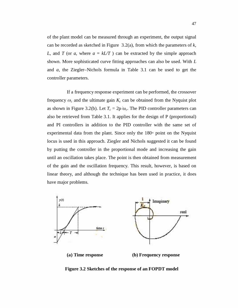
47

of the plant model can be measured through an experiment, the output signal

can be recorded as sketched in Figure 3.2(a), from which the parameters of k,

L, and T (or a, where a = kL/T ) can be extracted by the simple approach

shown. More sophisticated curve fitting approaches can also be used. With L

and a, the Ziegler–Nichols formula in Table 3.1 can be used to get the

controller parameters.

If a frequency response experiment can be performed, the crossover

frequency c and the ultimate gain Kc can be obtained from the Nyquist plot

as shown in Figure 3.2(b). Let Tc = 2p c. The PID controller parameters can

also be retrieved from Table 3.1. It applies for the design of P (proportional)

and PI controllers in addition to the PID controller with the same set of

experimental data from the plant. Since only the 180 point on the Nyquist

locus is used in this approach. Ziegler and Nichols suggested it can be found

by putting the controller in the proportional mode and increasing the gain

until an oscillation takes place. The point is then obtained from measurement

of the gain and the oscillation frequency. This result, however, is based on

linear theory, and although the technique has been used in practice, it does

have major problems.

(a) Time response (b) Frequency response

Figure 3.2 Sketches of the response of an FOPDT model

48

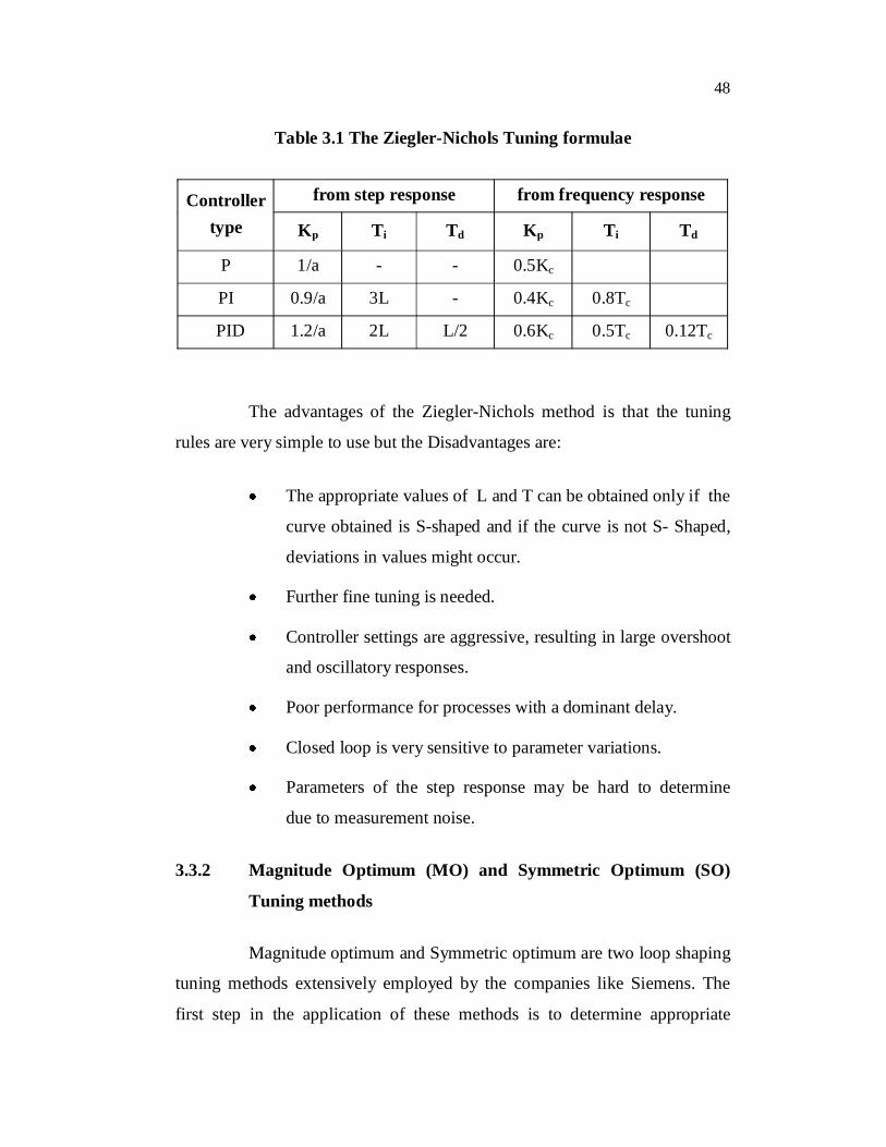
Table 3.1 The Ziegler-Nichols Tuning formulae

Controller type

from step response from frequency response

Kp Ti Td Kp Ti Td

P 1/a - - 0.5Kc

PI 0.9/a 3L - 0.4Kc 0.8Tc

PID 1.2/a 2L L/2 0.6Kc 0.5Tc 0.12Tc

The advantages of the Ziegler-Nichols method is that the tuning

rules are very simple to use but the Disadvantages are:

The appropriate values of L and T can be obtained only if the

curve obtained is S-shaped and if the curve is not S- Shaped,

deviations in values might occur.

Further fine tuning is needed.

Controller settings are aggressive, resulting in large overshoot

and oscillatory responses.

Poor performance for processes with a dominant delay.

Closed loop is very sensitive to parameter variations.

Parameters of the step response may be hard to determine

due to measurement noise.

3.3.2 Magnitude Optimum (MO) and Symmetric Optimum (SO)

Tuning methods

Magnitude optimum and Symmetric optimum are two loop shaping

tuning methods extensively employed by the companies like Siemens. The

first step in the application of these methods is to determine appropriate

49

transfer function which models the process. Once the transfer function is

determined, the controller is able to shape the open loop transfer function in a

desired manner. MO tuning method was devised with the objective to obtain a

control system with a frequency output characteristic as close to unity and as

flat as possible for the maximum bandwidth. Its mathematical expression

states the requirements posed on the closed loop transfer function Gc(s):

0)(sGc (3.6)

0))((

lim0 n

cn

djGd (3.7)

for as many n as possible.

Let the desired open loop transfer function is:

)2()(

2

1n

no ss

sG (3.8)

closed loop system and n determines the

closed loop dynamics, that is, the speed of response. For example, the PI

controller is employed when it is possible to approximate the model of the

process with the transfer function:

)1)(1()(

21 sTsTKsG p (3.9)

with T2<T1. By analyzing Equations (3.6) to (3.9) and by setting

Åstrom and

Hägglund, 1995).

22KTTK I

p (3.10)

TI = T1 n = 0.707/T2 (3.11)

50

The dominant pole is cancelled by the PI controller zero, and the

closed loop dynamics are determined with the smaller time constant T2 of the

process. MO design method optimizes the closed loop transfer function GC(s)

between the reference and the output signal. It often cancels the process poles

by the controller zeros, which can lead to poor performance of the control

system in response to load disturbance. The objective of the SO method,

which was originally proposed by Kessler (1958), is to obtain an open loop

transfer function.

)(

)()( 2

2

02c

cc

assa

sasG

(3.12)

where c is the gain crossover frequency and a is related to the phase margin

of the control system through:

11tan2

aaa (3.13)

or conversely through:

cossin1a

(3.14)

The method maximizes the phase margin of the control system and

leads to symmetrical phase and amplitude characteristics, as can be observed

in Figure 3.3.

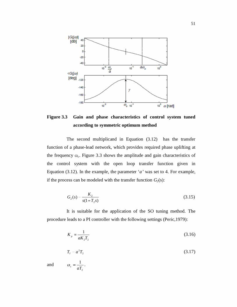
51

Figure 3.3 Gain and phase characteristics of control system tuned

according to symmetric optimum method

The second multiplicand in Equation (3.12) has the transfer

function of a phase-lead network, which provides required phase uplifting at

the frequency c. Figure 3.3 shows the amplitude and gain characteristics of

the control system with the open loop transfer function given in

Equation (3.12). In the example, the parameter ‘a’ was set to 4. For example,

if the process can be modeled with the transfer function G2(s):

)1()(

2

22 sTs

KsG (3.15)

It is suitable for the application of the SO tuning method. The

procedure leads to a PI controller with the following settings (Peric,1979):

22

1TaK

K p (3.16)

22TaTI (3.17)

and 2

1aTc .

52

The common choice for the parameter a is 2 which gives the phase

margin of the control system 37°.The SO method is designed to give a

good response to load disturbance, but the response of the control system to

set-point change has large overshoot. The overshoot is commonly reduced

through the usage of a two-degree-of-freedom controller or with a prefilter.

The MO and SO tuning methods are widely used in the cascade control

systems, especially to control motor drives (Peric 1979,1989) and

(Deur 1999).

As the controller tuning methods are available for second order

system hence model order reduction is preferred. The main objective of

model order reduction is to design a controller of lower order which can

effectively control the original higher order system. In the proposed scenario,

there are two common approaches for controller design. First approach is to

obtain the controller on the basis of reduced order model called process

reduction. In the second approach, the controller is designed for the original

higher order system and then the closed loop response of higher order

controller with original system is reduced pertaining to unity feedback.

Proportional Integral (PI) controller is designed for lower order model with

the help of proposed cross multiplication of polynomials model order

reduction method. This method is based on the minimization of the error

index criterion between the desired response and actual response pertaining to

a unit step input. The controller parameters Kp and Ki are obtained from the

reduced order model with the help of pole zero cancellation technique. Finally

this designed PI controller is connected to the original higher order system to

get the desired specification.

Genetic Algorithm was inspired by the mechanism of natural

selection called controller reduction. Both the approaches have their own

advantages and disadvantages. The process reduction approach is

53

computationally simpler as it deals with lower order model and controller but

at the same time errors are introduced in the design process as the reduction is

carried out at the early stages of design. In the controller reduction approach

error propagation is minimized as the design process is carried out at the final

stages of reduction but the approaches deal with higher order models and thus

introduce computational complexity. The Genetic Algorithm (GA) is

employed to reduce the mismatch between the given higher order and the

resulting reduced order models.

3.4 GENETIC ALGORITHM (GA)

The basic principles of Genetic Algorithm were first proposed by

Holland as a biological process in which stronger individual is likely to be the

winner in a competing environment. Genetic Algorithm uses a direct analogy

of such natural evolution to do global optimization in order to solve highly

complex problems. It presumes that the potential solution of a problem is an

individual and can be represented by a set of parameters (Sheroz Khan and

Salami Femi Abdulazeez 2008). These parameters are regarded as the genes

of a chromosome and can be structured by a string of concatenated values. This

form of variables representation is defined by the encoding scheme. The

variables can be represented by binary, real numbers, or other forms depending

on the application data. Its range ie., the search space is usually defined by the

problem. Genetic Algorithm has been successfully applied to many different

problems. It has also been applied to machine learning, dynamic control system

using learning rules and adaptive control (Pivonka 2002).

3.4.1 Genetic Algorithm Based Tuning of the PI Controller

In this thesis, Genetic Algorithm approach is used for the following

two purposes:

54

To reduce the error value between given higher order and

obtained reduced order models.

To determine the optimized value of PI controller parameters

namely Kp and Ki.

Genetic Algorithm is a stochastic global search method that mimics

the process of natural evolution. The genetic algorithm starts with no

knowledge of the correct solution and depends entirely on responses from its

environment and evolution operators (i.e. reproduction, crossover and

mutation) to arrive at the best solution. By starting at several independent

points and searching in parallel, the algorithm avoids local minima and

converging to sub optimal solutions. In this way, GA has been shown to be

capable of locating high performance areas in complex domains without

experiencing the difficulties associated with high dimensionality, as may

occur with gradient descend techniques or methods that rely on derivative

information (O’Mahony et al 2000). A genetic algorithm is typically

initialized with a random population consisting of between 20-100

individuals. This population (mating pool) is usually represented by a real-

valued number or a binary string called a chromosome. For illustrative

purposes, the rest of this section represents each chromosome as a binary

string. How well an individual performs a task is measured is assessed by the

objective function. The objective function assigns each individual a

corresponding number called its fitness. The fitness of each chromosome is

assessed and a survival of the fittest strategy is applied. In this thesis, the

magnitude of the error will be used to assess the fitness of each chromosome.

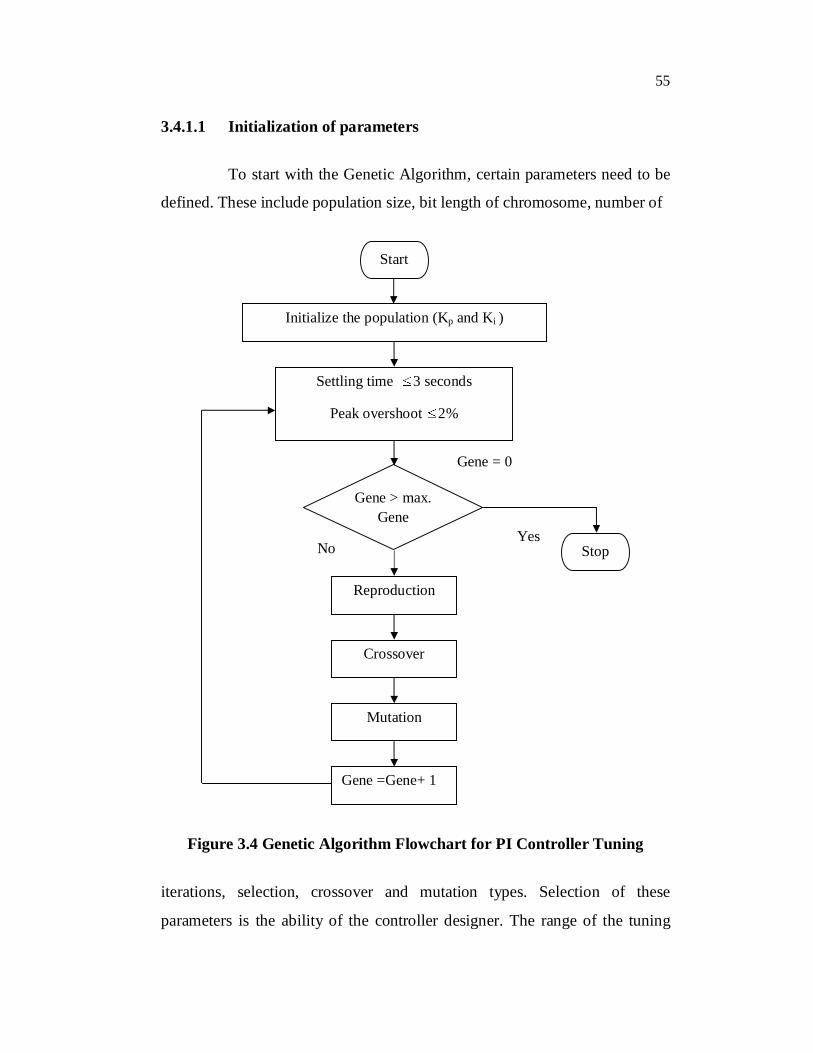
The flowchart for PID Controller tuning using GA is shown in Figure 3.4.

There are three main stages of a genetic algorithm, these are known as

reproduction, crossover and mutation.

55

3.4.1.1 Initialization of parameters

To start with the Genetic Algorithm, certain parameters need to be

defined. These include population size, bit length of chromosome, number of

Figure 3.4 Genetic Algorithm Flowchart for PI Controller Tuning

iterations, selection, crossover and mutation types. Selection of these

parameters is the ability of the controller designer. The range of the tuning

Start

Initialize the population (Kp and Ki )

Settling time 3 seconds

Peak overshoot 2%

StopYes

No

Reproduction

Crossover

Mutation

Gene =Gene+ 1

Gene > max. Gene

Gene = 0

56

parameters is considered between 0 and 10 (Mudi and Pal 1997). Initializing

values are detailed as follows:

Population type : Double vector

Population size : 100

Bit length of the

considered chromosome : 6

Number of generations : 100

Selection function : Tournament selection

Crossover type : Single point crossover

Crossover function : Intermediate

Crossover probability : 1.0

Mutation type : Uniform mutation

In each generation, the genetic operators are applied to selected

individuals (Kp and Ki ) from the current population in order to create a new

population (Mohammed Hassan and Waleed Sharif 2000). Generally, the

three main genetic operators of reproduction, crossover and mutation are

employed. By using different probabilities for applying these operators, the

speed of convergence can be controlled. Crossover and mutation operators

must be carefully designed, since their choice highly contributes to the

performance of the whole Genetic Algorithm (Ching-Chih Tsai and Chi-

Huang Lu 1998).

57

3.4.1.2 Reproduction

A part of the new population can be created by simply copying

without change, selected individuals from the present population. Also new

population has the possibility of selection by already developed solutions.

There are a number of other selection methods available and it is up to the

user to select the appropriate one for each process. Reproduction crossover

fraction is taken as 0.8

3.4.1.3 Crossover

New individuals are generally created as offspring of two parents

(i.e., crossover being a binary operator). One or more so called crossover

points are selected (usually at random) within the chromosome of each parent,

at the same place in each (Ismail Yusuf et al 2010). The parts delimited by

the crossover points are then interchanged between the parents. The

individuals resulting in this way are the offspring. Beyond one point and

multiple point crossover, there exist some crossover types. The so called

arithmetic crossover generates an offspring as a component wise linear

combination of the parents in latter phases of evolution. It is more desirable to

keep individuals intact and so it is a good idea to use an adaptively changing

crossover rate: higher rates in early phases and a lower rate at the end of the

Genetic Algorithm (Saravanakumar and Wahidha Banu 2006).

3.4.1.4 Mutation

A new individual is created by making modifications to one

selected individual. The modifications can consist of changing one or more

values in the representation or adding/deleting parts of the representation. In

Genetic Algorithm, mutation is a source of variability and too great a

mutation rate results in less efficient evolution, except in the case of

58

particularly simple problems (Mohammed Obaid Ali et al 2009). Hence,

mutation should be used sparingly because it is a random search operator;

otherwise, with high mutation rates, the algorithm will become little more

than a random search. Moreover, at different stages one may use different

mutation operators. At the beginning, mutation operators resulting in bigger

jumps in the search space might be preferred (Ali Reza Mehrabian and

Morteza Mohammad Zaheri 2003). Later on, when the solution is close by a

mutation operator leading to slighter shifts, the search space could be

favoured.

3.4.2 Summary of Genetic Algorithm Process

In this section, the process of Genetic Algorithm will be

summarized as a flowchart and is shown in Figure 3.5. The summary of the

process will be described below.

The steps involved in creating and implementing a genetic

algorithm:

Generate an initial, random population of individuals for a

fixed size.

Evaluate their fitness.

Select the fittest members of the population.

Reproduce using a probabilistic method.

Implement crossover operation on the reproduced

chromosomes.

Execute mutation operation with low probability.

Repeat step 2 until a predefined convergence criterion is met.

59

The convergence criterion of a genetic algorithm is a user specified

condition. For example, for the maximum number of generations or when the

string fitness value exceeds a certain threshold, they are considered as

terminating conditions.

Figure 3.5 General Flowchart for GA

3.4.3 Genetic Algorithm versus Traditional Methods

Genetic algorithm is substantially different to the more traditional

search and optimization techniques. The five main differences are:

Genetic algorithm search a population of points in parallel, not

from a single point.

Create/ Initialize Population

Measure/Evaluate Fitness

Select Fittest

Mutation

Crossover/Production

Optimum Solution Non Optimum

Solution

60

Genetic algorithm do not require derivative information or

other auxiliary knowledge; only the objective function and

corresponding fitness levels influence the direction of the

search.

Genetic algorithm use probabilistic transition rules and not

deterministic rules.

Genetic algorithm work on an encoding of a parameter set and

not the parameter set itself (except where real-valued

individuals are used).

Genetic algorithm may provide a number of potential

solutions to a given problem and the choice of the final is left

up to the user.

3.5 NUMERICAL ILLUSTRATION

Consider a fourth order system described by its transfer function

(Shamash 1975):

12018010218120090024814)( 234

23

ssssssssG

The corresponding reduced (2nd order) model obtained from the

preferred cross multiplication of polynomials method (as detailed in chapter

2) is obtained as,

253.1138.253.1298.11)( 2 ss

ssGr

Figure 3.6 shows the step response of the given higher order

system without controller. The controller parameters Kp, Ki and Kd are

determined from this step response by using the conventional Ziegler-Nichols

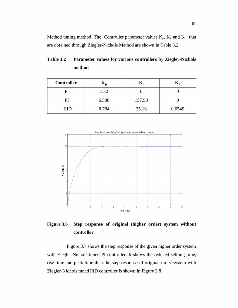
61

Method tuning method. The Controller parameter values Kp, Ki and Kd that

are obtained through Ziegler-Nichols Method are shown in Table 3.2.

Table 3.2 Parameter values for various controllers by Ziegler-Nichols

method

Controller Kp Ki Kd

P 7.32 0 0

PI 6.588 157.98 0

PID 8.784 35.16 0.0549

0 1 2 3 4 5 6 7 8 9 100

2

4

6

8

10

12Step Response of Original higher order system without controller

Time (sec)

Figure 3.6 Step response of original (higher order) system without

controller

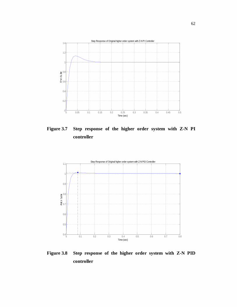
Figure 3.7 shows the step response of the given higher order system

with Ziegler-Nichols tuned PI controller. It shows the reduced settling time,

rise time and peak time than the step response of original order system with

Ziegler-Nichols tuned PID controller is shown in Figure 3.8.

62

0 0.05 0.1 0.15 0.2 0.25 0.3 0.35 0.4 0.45 0.50

0.2

0.4

0.6

0.8

1

1.2

1.4Step Response of Original higher order system with Z-N PI Controller

Time (sec)

Figure 3.7 Step response of the higher order system with Z-N PI

controller

Step Response of Original higher order system with Z-N PID Controller

Time (sec)0 0.1 0.2 0.3 0.4 0.5 0.6 0.7 0.8

0.4

0.5

0.6

0.7

0.8

0.9

1

1.1

Figure 3.8 Step response of the higher order system with Z-N PID

controller

63

The best population may be plotted to give an insight into how the

genetic Algorithm converged to its final values as illustrated in Figure 3.9.

The step response of the original higher order system with PID controller is

shown in Figure 3.10.The GA tuning of the reduced order transfer function

results in the following Controller parameter values: Kd = 1.00404,

Kp = 22.84908 and Ki = 25.6977. Using these controller parameters, the

higher order system is tuned and the step response of the higher order system

with GA based PI controller is shown in Figure 3.11. The step response of

the reduced order system with GA PI controller is shown in Figure 3.12.The

Step response of the reduced order system with GA PID controller is shown

in Figure 3.13. The Step response of the reduced order system with Z-N PID

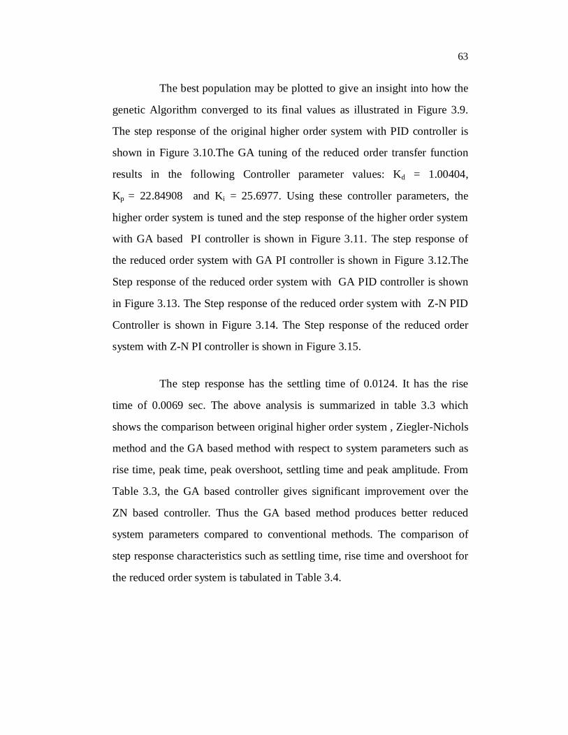
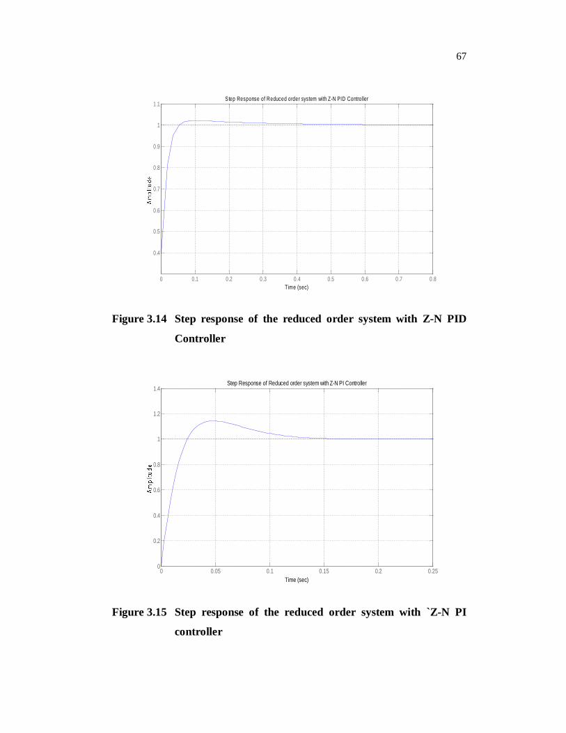
Controller is shown in Figure 3.14. The Step response of the reduced order

system with Z-N PI controller is shown in Figure 3.15.

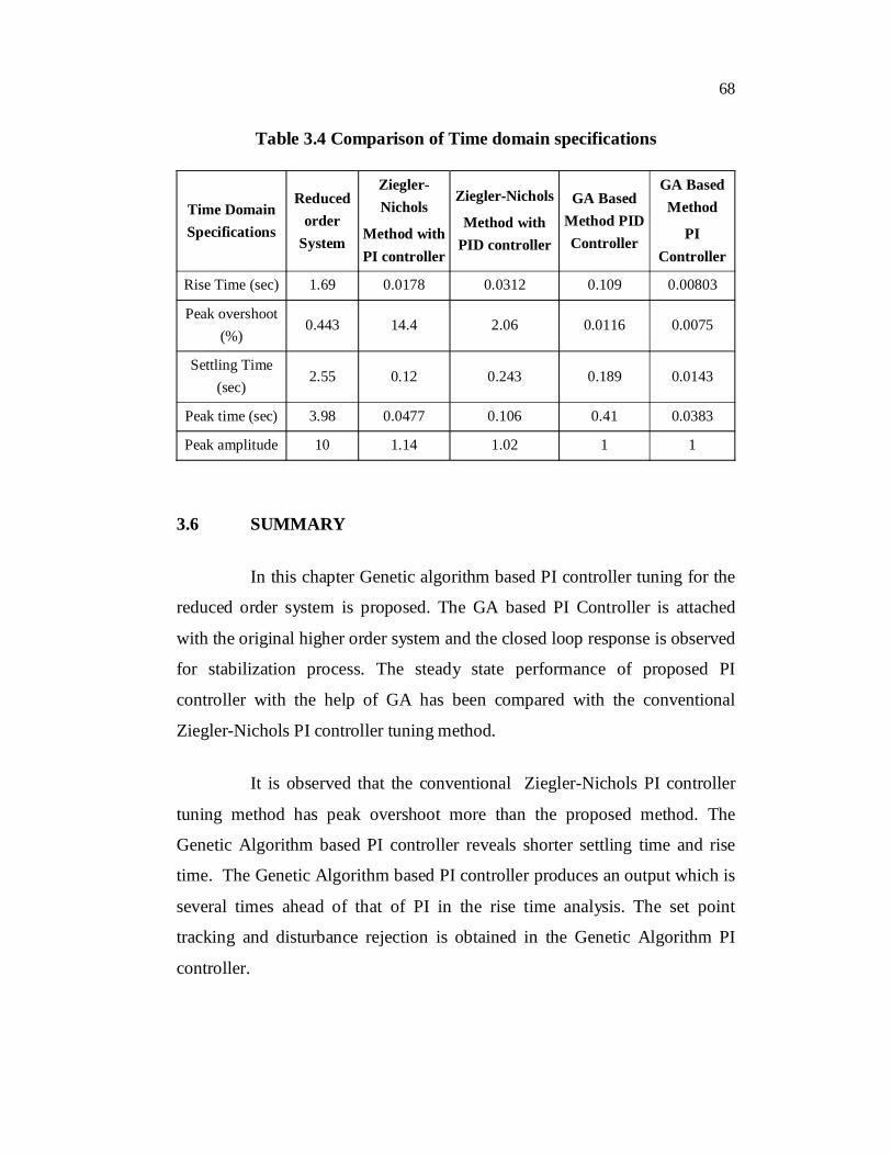
The step response has the settling time of 0.0124. It has the rise

time of 0.0069 sec. The above analysis is summarized in table 3.3 which

shows the comparison between original higher order system , Ziegler-Nichols

method and the GA based method with respect to system parameters such as

rise time, peak time, peak overshoot, settling time and peak amplitude. From

Table 3.3, the GA based controller gives significant improvement over the

ZN based controller. Thus the GA based method produces better reduced

system parameters compared to conventional methods. The comparison of

step response characteristics such as settling time, rise time and overshoot for

the reduced order system is tabulated in Table 3.4.

64

0 50 100 150 200 25015

20

25Kp Value

0 50 100 150 200 25025

30

35Ki Value

0 50 100 150 200 2500

2

4Kd Value

Generations

Figure 3.9 PID controller parameters tuning process using GA

0 5 10 15 20 25 300.93

0.94

0.95

0.96

0.97

0.98

0.99

1

1.01Step Response of Original higher order system with GA PID Controller

Time (sec)

Figure 3.10 Step response of the original higher order system with GA

PID controller

65

Step Response of Original Higher order system with GA PI Controller

Time (sec)0 0.01 0.02 0.03 0.04 0.05 0.06 0.07

0

0.2

0.4

0.6

0.8

1

Figure 3.11 Step response of the original higher order system with GA

PI controller

Table 3.3 Comparison of Time domain specifications

Time Domain Specifications

Higher Order System

Ziegler-Nichols

Method with PI

controller

Ziegler-Nichols

Method with PID

controller

GA Based Method

PID Controller

GA Based

Method

PI

Rise Time (sec) 1.69 0.0157 0.0285 0.122 0.0069

Peak overshoot (%)

0.443 13 1.4 0.0405 0.061

Settling Time (sec)

2.55 0.107 0.12 0.398 0.0124

Peak time (sec) 3.98 0.0409 0.0815 0.97 0.0266

Peak amplitude 10 1.13 1.01 1 1

66

Step Response of reduced order system with GA based PI Controller

Time (sec)0 0.01 0.02 0.03 0.04 0.05 0.06 0.07 0.08 0.09 0.1

0

0.2

0.4

0.6

0.8

1

Figure 3.12 Step response of the reduced order system with GA PI

controller

0 0.05 0.1 0.15 0.2 0.25 0.3 0.35 0.4 0.45 0.50.92

0.93

0.94

0.95

0.96

0.97

0.98

0.99

1

1.01Step Response of Reduced order system with GA based PID controller

Time (sec)

Figure 3.13 Step response of the reduced order system with GA PID

controller

67

0 0.1 0.2 0.3 0.4 0.5 0.6 0.7 0.8

0.4

0.5

0.6

0.7

0.8

0.9

1

1.1Step Response of Reduced order system with Z-N PID Controller

Time (sec)

Figure 3.14 Step response of the reduced order system with Z-N PID

Controller

0 0.05 0.1 0.15 0.2 0.250

0.2

0.4

0.6

0.8

1

1.2

1.4Step Response of Reduced order system with Z-N PI Controller

Time (sec)

Figure 3.15 Step response of the reduced order system with `Z-N PI

controller

68

Table 3.4 Comparison of Time domain specifications

Time Domain Specifications

Reduced order

System

Ziegler-Nichols

Method with PI controller

Ziegler-Nichols

Method with PID controller

GA Based Method PID Controller

GA Based Method

PI Controller

Rise Time (sec) 1.69 0.0178 0.0312 0.109 0.00803

Peak overshoot (%)

0.443 14.4 2.06 0.0116 0.0075

Settling Time (sec)

2.55 0.12 0.243 0.189 0.0143

Peak time (sec) 3.98 0.0477 0.106 0.41 0.0383

Peak amplitude 10 1.14 1.02 1 1

3.6 SUMMARY

In this chapter Genetic algorithm based PI controller tuning for the

reduced order system is proposed. The GA based PI Controller is attached

with the original higher order system and the closed loop response is observed

for stabilization process. The steady state performance of proposed PI

controller with the help of GA has been compared with the conventional

Ziegler-Nichols PI controller tuning method.

It is observed that the conventional Ziegler-Nichols PI controller

tuning method has peak overshoot more than the proposed method. The

Genetic Algorithm based PI controller reveals shorter settling time and rise

time. The Genetic Algorithm based PI controller produces an output which is

several times ahead of that of PI in the rise time analysis. The set point

tracking and disturbance rejection is obtained in the Genetic Algorithm PI

controller.