Embed Size (px)
Citation preview

CHAPTER 3
Optimizatior~ of Process Parameters
3.1 Introduction
The liberalization of ninrket economics and suhscquent global competition has
made tlie entsepreneiirs to realize tlie impel-tancc of cjuality goods at affordable price.
One of the kcy areas iticntifird to rcaiize this objecti\.e is parameter optimization.
In\estigatio~is indicate that in the grii~ciing process dcptli o f cut, numhcr ofpnsses, \vheel
spccd and \ ~ o r l i speed ni-e the iiiqjor influential pal.al11ett.r~ \ihich affect the clualiry o f
the part grounded. In this cliaptzl thc studies contiuctcil to e\ aluate tlie effect of various
process parametci-s on tlie attainable surt'ace rougiint.:;~ an t i surt'zice hard~lcss are
presented. Tlie primary ol?iecri\,c of this study is to implement Taguchi 's Quality
engineering concept for the process variables optilnizatioli of grinding process.
Experiments are coiiducted according to Taguchi's LC) orthogonal array. Optirnum
grinding co~lditioils are a l ~ i v e d by einploying lower surface rouglzness c u ~ u higher
surface hardness are better as the strategy. The Secondary objective is to develop an
ANN systen: to integrate the ATN model with Taguchi 's model.
3.2 Selection of grinding wheel
Two problems, ~ilheel glazing and wheel loading occur in grinding process due to
wrorig selectio~i of grinding ~&i l~ee l or improper cutting conditions. Wheel glazing refers
to the co1:ditiol:s when the grains are worn dowil to the level of bond and held for too
long for grinding the matel-ial. The problem can be remedied either by changing the
wheel or by c l ~ a n g i ~ l g the cutting conditions. Wheel loading occurs urhen uol-l< piece
chips are embedded in the cutting Face of t l ~ e wheel, wl?icli reduces the effective depth of
penetration of the wheel abrasive into the work surface and thereby reducing the rate o f
cutting. Wheel loading is aggravated b y the presence of small voids o n the face of the
g~iniiing \i.lic.cl .-l'ki> < > i i 'ilc ciircil i>> :!>ci.c;ising the \\~hceI speeti or usiiig different wheel
e \ 211.
T i~us , the seiection of' grinding \i.ileei f :. correct, cor~tinuous efficient cutting
dcii~ands the correct se1cc:ioi: 01' tlic ty?e of abrasi\.e. the size 01' grains. and the type o f
boniiing agents and its s~rt.ngth nilti the size of \.(>ids. FLII-tiler, the behaviors of the
grinding v:liczls are ai'fcctccl by tilo work piece materials, cutting speed, depth o f cut and
the feed rate.
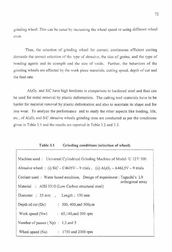
A1203 and SIC have high hardness in comparison to ha]-dcned steel and thus can
be ilsed for metal remoi a1 by plastic defoimatioii. The cutting tool Inaterials have to b e
harder for material removal by plastic deformation and also to maintain its shape and for
less wear. To analyze the per fo~mancr and to study the othzl- aspects like loading, life.
rtc.. o f 4 1 2 0 ; and SIC abrasive \vheels grinding tests are conducted as per the conditions
given in Table 3 . I and the results arc reportcd in Table 3.2 and 3.3.
Table 3.1 Grinding conditions (selection of wheel) --
Ivlacliine used : Uiliversal Cylindrical Grinding Machille of .Model U 127' 500
Abrasive wheel : (i) S i c - C3615V - 9 trials , (ii) A1203 - .r\46L5V - 9 trials
Coolant used : Water based emulsion. Design of experiment : Taguchi's L9 01-thogonal array
Material : AISI 33 10 (Low Carbon structural steel)
Diameter ; 35 inn1 , Length ; 150 111nl
Depth of cut (Dc) : 300.400,and 500pm
Work speed (Nw) : 65,140,and 300 i -p~~l
Number of passes ( Xp) : 1.3,and 5
Wheel speed (Ks) : 1750 and 2000 iyrn

Table 3.2 Orthogonal at-ray of grinding parameters and test results
--- (.AIISI 3310 \\ith SiC \ ~ h e e l ) I Ra in p111 1 Average
I DCII: Nn ~ i i hs 111 1 Ra I S NO. 1 Np -- 1 1 kin1 ~ I I I I 1;)m , 1 T---, I 11 1 I I I I value I
I I I I trial tnnl ~, trial 111 pn1
I 1750 I 0 10 0 18 0 17 0 17 - - - _ _ _ --
07 , 3 00 1 40 3 7000 0 15 0 14 -------
03 i 300 300 5 7000 O i l 000 01-3 0 1 1
Table 3.3 Orthogonal array of grinding parameters and test results (AISI 3310 \tit11 A1203 wheel)
I
Rn in pln Average

Ti12 a\cl.:igt ei'fci-!s ~ i ' ~ i l ; \ i i : !'i!ctors oil ~ L I ~ I ~ I C C ~.oiiglilicss are gi\-eil in Table 3.4
snc! 3.5 ii)r the c o ~ l ~ h i ~ i a t i i ~ ~ ; 0 1 ' . i lSl 7.2iO \ii!Il SIC an(! .%IS1 3310 wit11 A1203
respecti\ el!.
ANOVA ana!ysis is carried oLii i~ driznnii~t ' the influrncc of 111ain factors and to
dctcrmine the percentage contribution of each t'actol.. Tabie 3.6 sho\i~s the results of
percentage contributiixl ofeacll factor.
The clerails of caiculation to find tile aicrttge cffect of main factors on surface
~.oughnt.ss at three difii.1-cnt Ic\,cls. percentage contriburiou of' tach facial- on surface
1.oughness. and optimum surface roug1111ess estiliiation tbr the ~vliezl \vol.l< combination of
AISI 3310 with AI2o3 wheel a r c given beion'.
Average surface roughness value f o r the parameter dep th of cu t a t each level
Low level (300 pm) Ra =(0.14+ 0.12+ 0.09)i 3 = 0.1 167
Medium level (400 pm) Ra = (0. !2+ 0. I5+ 0.1 X).' 3 = 0.1467
High level (500pm) R a = (0.12+ 0.15+ 0.18)i 3 = 0.15
Similarly, for Number of passes, Wliesl speed, and work speed the average effect
on surface roughness is calculated.
ANOVA analysis to find the percentage contr ibut ion of each fac tor
Correctioll Factor,
CF=(0.14+0.12-0.09-0.12+0.15+ 0.18 +0.12+ 0.15+ 0.18) ' i 9
= 0.1708
Sum of squares,
S T = (0.14'+ 0.12'+ 0.09' -0.12~+ 0.15'+ 0.18 '+0 .12~+ 0.1j2+ 0.18') - CF

ST = ~),00005~>
SLII :~ O ~ ' S L ~ U ~ I I . C S liw tii'j>til ~ ~ ' C L I I .
SDc = -?((I. 1 1672-*- 0 . 1 - 0. ! 5 ' ) 0. 170s
SDc = 0.002022
Similarly for i7tht.1- pai.amctcrs [hi. suiil of sclu:jl-e ia ~aiculnted.
S N w = 0.001)8272, S N 17 = ij.002132, S N s = 0.OCI I089
En-or sun? ofsquai-es is :ilso c:ilculated.
Error sum of scjuarcs SE ST- ( S DciS N\\.- S K p- S N S ) = 0.0006
Percentage error = SE .' ST' = S.626?6
Percentage influence of ciepth of cut = SDc, ST * I00 = 29.07U/b
Similarly for other parameters thc percentage conti.ibution is calculated.
Work speed - 11.82%. Numl~ei- of passes - 34.82"/0. Whcel speed - 15.651/0
Optimum condition for surface I-ough~less
Lotver surface ro~~gliness is better as the strategy is ibllowed. 111 table 3.5 and 3.6
the lo~vtfs values of surface roughiicts!: are liigliligl~ted ancl thc co~.rcsponding Levels of the
parameiers constitute the Optin~uni treatment cornhination.
Optimr~m surface I-oughness
Ra mean = (0.14+ 0.12- 0.09 -0.12+ 0.15+ 0.18 +0.12+ 0.15+ 0.18) / 9
= 0.1378
Optimum conlbination - Average surface roughness values
Depth of cut (Low level) - 0.1 167
Workspeed (Low level) - 0.1267
Number of passes (High level) - 0.11 67
Wheel speed (High level) - 0.17 17
Ra optimum = Ra mean + i(0.1167-0.1378) - (0.1267-0.1378) t (0.1 167- 0.1378)
- (0.17 17-0.1378)) = 0.07667

T:~blc 3.4 .\\ el-age effcct of main factors on surface I-oughness (.%IS1 3310 nit11 Sic n heel) ---
.A\ c ~ , ~ g i . Ra \ a lu r for maln factors at ,
Table 3.5 Average effect of main factors on surface roughness (AISI 3310 with AlzOz wheel)
Xael-age Ra value for maiil factors at
I 1 Lr\.el 2 I Level 3
1 - Number of Passes 1
I 0.1567 ~ 4 v l
Work speed
Table 3.6 Percentage contl.ibution of each factor on surface roughness (AISI 3310 with A1203 1 S i c wheel)
Parameters AISI 33 10 1 AISI 33 10
with SIC with A1203
I I
Number of Passes
Wheel speed
En-or
44.34% , 34.82%
14.48% 15.65%
06.1 00/0 08.63% I I I

Optii11un-i conciition si~l.fjcc ~-c~ugIrness for boih tile \vIleel anti work
combination is foiind b adopting thc lo\i.er ss!ri.ice roughness is better as the sti.atcgy
nnci results are gi\en i!nde~..
( i ) Depth of' cut at Lel.el 1 (3OOum)
(ii) Work speed at Level I (65 ipm)
(iii) Nunibcr of passes at Level 3 ( 5 passes)
t i \ : ) Wheel s p e d ai Le~.el 2 (2i)OO I-pm)
Opt~mum \usi'Llce rougJi~i~ss nluc is
( i j For AISI 33 10 \\.it11 S iC - 0.098~m
( i i ) For AiSI 33 10 with .4i2@ - 0.077~irn
This study shows that the SIC gives a pool- susfiice kinis11 on steel work
materials like the ones used in this woi-k because of its high hardness( Table 3.2 and 3.3).
Further, it is observed that, with SIC wheel there is a loss of cutting efticieilcy
accompanied by the appearance of chatter marks on the work surface after grinding a few
pieces. And also, the work ~uaterials used in this research \vosk are of high tensile in
nature. These materials offer inore resistance to machining preceded by plastic
deforillation with SiC wheel. More over. SIC abrasi1.e~ being more brittle in nature. they
fall of rapidly due to quick fi-actures resulting in frequent wileel dl-essing. Because of the
above mentioned reasons, A120; grinding wheel oi'specificntio~l A46L5V is selected and
used for all rile expesimeilts in tiis study.
3.3 Comparison of design of experiments
Changing denlands of dynamic inarket place ha1.e improved and increased the
commitment to quality consciousness. All over the world, companies are developing
quality management systeills like IS0 9001-2000 and investing in total qualit>. One of
. ,
ijie ;!-iti~ai rCi!~ii:~c!i;c~;r.; lo? ? I I C IS0 Ol!Ol-2!jOO is ntlcc~ilnrr control ot.c.1' process
I L ' ~ I L C t i i i i ! I i s .-in auditing l.el)ort of
ijie [SO indicates tilax :he ~:~;ijol.it~ O I ' I ~ ~ L ' i ~ l a ~ ~ ~ i f . i ~ ~ t i i r i ~ ~ g ili(iusti->. pl-esents the improper
c~ppiication of proccss 1-ai.inb!cs an<! inadzcjuate control o\.er t i i t : process parametel-s.
Co:i!sc>i of process paralnete~. is possibIc ti~l.ough <,ptimization 01' process vat-iables.
Dctzrn?ination of' opt imum p:il-;i~i:t.tcrs lies in tile proper selection and intsociuction of
suitable design ni'cspcriment at tile cai.licst strife ot'the process aild product developlnent
c\.,cies so as to restilt in the quality and p~.oducti\,ity impro\.eineni.
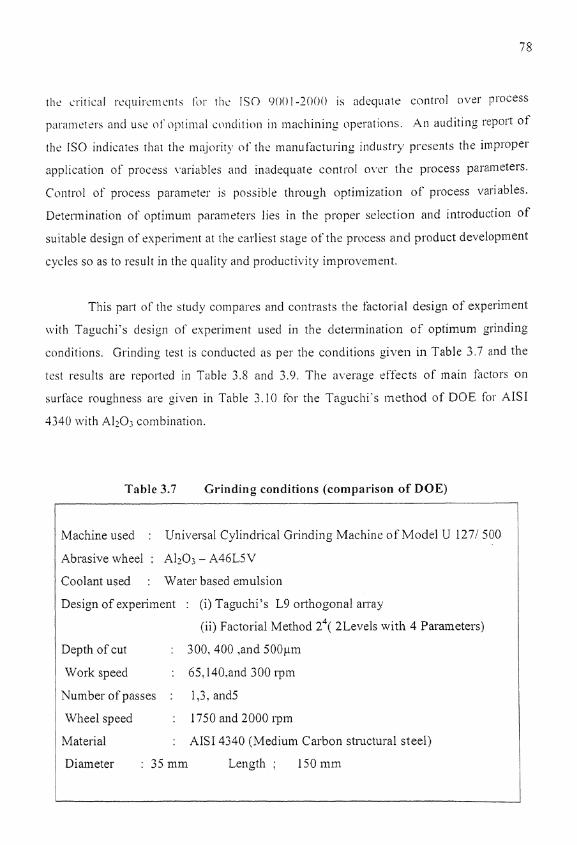
This part of the study cornpal-es and contrasts the factorial design of experiment
\vith Taguchi's design 01' experiment ~ised in the detei-mination of optimum grinding
conditions. GI-inding test is conducted as per the conciitioils gi\,en in Table -3.7 and the
tcst res~111s are rcported in Table -3.8 and 3.9. Tile avzragc cffects of main factors on
surface rouglincss are gi\.en in Table 3.10 for the Taguclli's method of DOE Ibr AISI
4340 with Ai20; coml?i~iation.
Table 3.7 Grinding conditions (cornpal-ison of DOE)
Machine used : Universal Cylindrical Grinding Macl~i r~c of Model U 127.' 500
Abrasive wheel : Al7Oj - A46L5V
Coolant used : Water based elnulsion
Design of experiment : (i) Taguchi's L9 orthogonal al-1-ay
(ii) Factorial Method 2'( 2Levels with 4 Parameters)
Depth of cut : 300.400 ,and 50011111
Work speed : 65.140,and 300 l-pm
Nuniber of passes : 1,3. a11d.5
Wheel speed : 1750 and 2000 1l3m
Material : AISI 4340 (Medium Carbon structural steel)
Dialneter : 35 111m Length ; 150 mm

Tallle 3.8 Classical design arm! of grinding paranleters arid test results
(&IS1 1310 \\it11 .4120; - Z~ Factorial n3ethod)
I Ra in kin1 1 .A\.e~.;~gt. : SDS APD DL i XI\, Ss
I . , Ra i~~c t i iod method S N O i i \ p i i l -___- 7---
I I I l l i l l i a i u e R a i n I R a i n hiin 1 rpm ~ p m ,
I I I , trial trial trial i i pm 1 urn

AKOVA ailalysis is carried out to detellniile the influence of main factors and to
detelnline the percentage contribution of each factol-. Table 3.1 1 sho~bs the results of
percentage contributioll of each factor.
Table 3.9 0rthogom:~l arm! of grinding parameters and test results
I Average I
8 Dcin hiiirl S No
, j i l l l Ipnl I !
-+
Table 3.10 Average effect of main factors on surface roughness
01 1 300 65 I 7 0 , 0 i 5 ' 0 13 0 14
(AISI 4340 with ,4I2o3 - L9 Tsguchi's method) Average Ra value for iliaill i'acrors at three
0 14 ~
Parameters I ie\/els i
00 140 3 0 I . 0 2 0 1 0 0 1 2 1
I ____I
Depth of cut / 0.1 167 0.1367 1 0.1533
Work speed
Number of Passes
Wheel speed
0.1267
0.16
0.1533
0.14 0.15
0.14 0.1 167
!
0.1317 1 I

Tahle 3.1 1 Pcrceritagc cont r i l~~r t ion of each factor on surf'ace roughness (-IISI 4310 v i t i l 111:03 - Factorial !'s Tagucl~i 's n~ethod) ---
I I Par3meti.l.s Taguchi's metiloci Factorial method I
i
Work speed 11.28O0 ~ 1 1.82% 1
I Errol- 0572 ' !h 08.63% I ,
Optilnurn condition for surface roughr~ess obtained il l the Taguchi's method
adopting the lo& er is better strategy and thc results arc gi\.en ul~tier.
( i j Depth oi'cut at Lc\.rl i j3OOpm)
(ii) Work specti at i-c\,el I (65 i p ~ n )
( i i i j S~111117er OS~I:ISS~S at Le\.el 3 ( 5 passcs)
( i ) Wheei speed at Lew! 2 (1000 11-1rn)
Optimu~ll surface roughness ~ a l u e for AISI 4340 is 0.075pm 111 Taguchi's
i ~ ~ e t h o d .
In factorial method, regression analysis IS done uslng EES software by applying
Sum of Deviation Square inethod (SDS) and Average Percentage Deviation method
(APD). The regression model (equation) so obtained to predict surface roughness is
A = 0.000021871, B = -- 0.002753973, C = -- 0.000078756, D = 0.000074365 (SDS)
A = 0.000028024, B = -- 0.003117953, C = -- 0.000089156, D = 0.000071569 (APD)
In the above equation the values of input parameters call directly be substituted
and the surface roughness can be deteinlined.

Both of t!le desip:) nf espc.riinc~~t stuciics re\-eal that thc depth of cut and number
01 ' passus are ha! ing more ii:t!ucncc i r i l tl1.t. surihce t inis l~. Tnguclii's ~net l iod g k e s the
op:irnum gl-inciing contiitiol~s tiircc!l~- r~nci inturli the optimum grinding conditions can be
utilized t i7 ca1c~:latc the gi.intiing q .c le t in~e . Tliis iiifcrence is not possible lvith Factorial
~:~i.tliotl and i t is lilso to he r:oti.d ti lnt t ! ~ c i'rictorial nit.tIioi1 titkcs 11i0i.e trials to give the
r.'sulrs. Fu~.tlirr. F2ictorial 11ic.tllcttl lint! Taguciii's nietlioti gi\-c the saliie results on the
pcrcenragc int!uen.cs ol'e;1c11 paramcirr oil surf~icc roug!~i:css. Hence. Taguchi's method
i>i ' design of ctxperimciit can bc applieci to optimize tile process par~umeters \\.it11 added
ad\,nntnge of sa\,iilg t!~c tiine.
3.4 Grinding performance
Grinding performance differ from machine to macl~ine even when same
~i;oricmateriai and saine v,.heel ~naterial are uscd. In order to fix the type of 111achine best
suited for this complete research war!<. a perfolmance comparison is made between
universal cylindrical grinding n~achine and high precision plunge type cylindrical
grinding macliine. The grinding conditions and the lzst results a]-e given in Table 3.12.
3.13 and 3.14 respecti\rely. The n\.erage effects of main factors on surface ~ O U ~ I I I I C S S are
gi\,en in Table 3.15 and 3.16 for rhe blacl~ine ( i ) and Machine ( i i ) for the combination of
AISI 1040 ~vorkmaterial lvith A1:0: !vl~eel abrasivct material.
Tahle 3.12 Grinding conditions (Selection of machine)
Machine used : ( i ) Universal Cylindrical Grinding Machine 01' Model U 127: 500
(ii) High precision plunge type cylindrical Grinding Machine of
Model UCG 2601350 unit 500
Abrasive wheel : AlzOj - A46L5V ,Coolant used: Water based ernulsion
Material : AISI 1040 , Dia meter ; 35mm , Length ; 150 1i1m
Design of experilllent : Taguchi's L9 01-thogonal array
Depth of cut : 200, 400 and 600yin, Number of passes: 2,4,and 6
Machine (i) Machine (ii)
Work speed : 65,140,and 300 ipm Worli speed : 56,225,and 450 i-pm
Wheel speed : 1750 and 2000 rpln Wheel speed : 1550 and 1740 l-pm

'Table 3.13 Orthogonal :lt-ra? of grillding pal-anieters and test results (.%IS1 1040 -- nith -\IZ03 - llacktir~e ( i ) / Uni\ cl-sal)
I I ICa in ,ULII I Aberagz I
I Dciii S i i . i i 3 i Ns ill : value 1 S.No. 1 -
p In q,rn
I 1 I I
I Dcin Nw in i N s i n 1 value S.No. 1 I
11p1n I 11 I11 Ra in
I trial trial trial p111 ----
2 1550 0.15 0.16 0.14 0.15
Table 3.14 Orthogonal array of grinding parameters and test results (AISI 1040 with Ai2Q3 - Machine (ii) / Plunge)
1 I
I I
Ra in urn 1 Avciage

Tahlc 3.15 ;i\cl-agc cfl'cct of taaai11 factors on surface roughness (,-lISl 1040 ~ j i t h ..i1203 - J l ; ~ c I ~ i r ~ c ( i ) i L-rii\.crsal)
-- -- - -. - i ic ragi ' Ra i niilc k)l- lnain factors a1 i
- -- .- ---- Lei ti I ~ c . l e l 2 T T e T
\\heel speed 0 190 0 1717
Table 3.16 A ~ e r a g e effect of main factors on surface roughness (AISI 1010 nit11 A1201 - RIachine (ii) I Plunge) --
I : . \si.rageRa la luc ji71 llialli ractot~ at
I Parameters I i ! tl~ree Ie\,els I 1
I I Lcscl 1 ~ c ~ c l 2 ~ e v e l 3
-- . - -?-
~ o r ~ < speed 0. 1367 0.15 0 16 ,
XNOVA analysis is carried out to determine the influence of main factors and to
dete~mine the percentage contribution of each factor. Table 3.17 shows the results of
percentage contribution of each fact01
I Work speed ' 09.49% 09.92" 1
Table 3.17Percentage contribution of each factor on surface roughness (AISI 1040 with A1203 - Universal 1 Plunge)
Para~neters I Machine(1) I
I
Machine(il)
Number of Passes 43.05% 1 39.68% I
Depth of cut I
30 85% , 37.27%
Wheel speed 10.25% 11.33% ,

Optimum conilition fbr juriiici. rougi~ness for both tiic muchines ( i and i i ) is found
bx atiapting tile loncr is lxtter straicgL. and given under the Tabit. 3.18.
Table 3.18 O p t i n ~ u n l conditions f o r sur face roughness
(:\ISI 104O \\ it11 .4lzO3 - Ul~ir,crsal / Plunge)
I Pal ameten hlachine(i) Mncli~ne(ii) I - I Depth of cut 100pm 100pn1
1 humber of. Passcs 6 pa\ws 6 passes I
1 Wheel speed 2000 ~ p m 1 1740 i-pm
Optimum surface roughness value for AISI 1010 with h1203 in
Machine (i) universal - 0.1 183um and
Machine (ii) plunge -- 0.08 17pm.
'4 propel- selection of grinding machine could result in tlie in~provement of surface
quality. retained strength. tolerances /finish. production rate. cost per part, and product
performance of grounded components. Tilest results arc nlostly affected by the macl~ine
tool factors such as rigidity. precision, dynamic stability, controls, powerlspeed, slide
moven~ents/axles, truing and dressing equipment, coolant type. pressure, flow ztc.
Table 3.13 and 3.14 coinpare the surface finish results obtained fiom universal
and plunge type cylindrical grinding machine. They show that machine (ii) performs
better. Further, the optiinum surface roughness value is lesser in the case of Machine (ii)
and also the optimu~n condition obtained for machine (ii) indicates that the grinding cycle
time is lesser. Hence, considering the facility of Multi diameter grinding and other
advantages of Plunge type Cylindrical Grinding n~achine over the Universal Cylindrical
grinding machine. Pluilge type is prefened and selected to conduct experiments in this
study.
3.5 Opt imi~at ion using l'nguchi's Slethotl
The idea oi'statisticaliy ilesigneti ~xpcri inents to investigate pi-ocess variables and
their effects 011 p1.oduct q u a l i r characteristics has been around since the 1920's.
promoted largely by the great Sir Ronalti A. Fisher. who \<,as knighted for his creative
accomplishments in rhis iield. Taguchi's method emphasizes the use o f statistically
designed zxperim~'nts as a n~cans of tnhilncing tile quality of design o f products a i d the
pt.rii,~.mailce of procluc~ioii PI-occsses. >lost process control techniques lxeasure one or
inore output qua!ity cl~asactcristics. and if'these quality zhnl.ncteristics arc satisfactory. no
modification of the process is matic. I-io\vc\.er. in soi-i~i. situations \\rhei-c there is a strong
reln~ionship betn,ccli one 01. more controllable intiepcndcnt \.arinbles, other process
contsoi methods can so~notimes be employeci.
In this study Taguchi's 01-thogonal array of design of experiment is introduced in
a cylindrical grinding process for the optimization of process variables to improve the
quality of a ground surface. The experiments are conducted to study the influence of'
process parameters on surface roughness anci surface hardness as per Taguchi 's DOE.
Three different optimization analyses are done for different matel-ials. The detailed
procedures are given under.
Three different carbon percentage AISI steel materials are taken for this analysis
namely AISI 8620, .&IS1 H 1 1 . and AISI T I . AISI 8620 (low carbon) is subjected to fine
grinding with depths of cut 100,200 and 300 pi11 following the LO experimentation.
Optimizatioil is done using the Response graph method. The optirliizatioll results
obtained are coinpared and verified with Six ratio analysis and grey relational analysis.
AISI H I I (medium carbon) is subjected for nlediuin fine griilding test with depths of cut
200,300, and 400 urn. A detailed signal to noise ratio analysis is carried out to predict the
best treatment coillbination out of the nine trials conducted. Similarly, for AISI T 1
material with higher depth of cut (300,400 and 500pm) the grinding results are analyzed
using grey relational technique.

3.5.1 Optimization using Taguchi's Method b~ith Response Graph analysis
Tapch i essentially utilizes the conventional statistical tools, but he simplifies
them by identifying a set of stringent guide!ines for experiment layout and analysis of
results. Response graph analysis gives the output of interest to be optimized i.e.
minimized, maximized, targeted, etc.The output can be more than one and also it can be
quantitative or qualitative. The grinding conditions adopted in the experimentation are
given in Table 3.19, and the test results are reported in Table 3.20
Table 3.19 Grinding conditions for AISI 8620 (Response graph analysis)
/ Machine used : High precision plunge type cylindrical Grinding Machine of I 1 Model UCG 2601350 unit500 I Abrasive wheel : A1203 - A46L5V, Coolant used : Water based emulsion
Design of experiment : Taguchi's L9 orthogonal array with Response Graph method
analysis, Material : AISI 8620 (Low Carbon case carburising steel)
Depth of cut : 100, 200,and 300 pm , Number of passes : 1,2,and 3 , Length : l5Omrn
I Work speed : 56,225,and 450 rpm , Wheel speed : 1550and1740 rpm ,Dia : 35 mm I
Table 3.20 Orthogonal array of grinding parameters and test results (AISI 8620 with A12O3 - Response graph analysis)
S.No.
01
Dc
in
Pm
100
Nw
in
rPm
56
Np
1
Ns in
Surface roughness Ra in prn
Surface hardness in
HRA iI
trial
0.14
rpm I I
Average
Ra
I
trial
32 1550
Average
HRA
11
trial
3 3
value 1 trial
0.13
in pm
0.14 32

The a\.eragc c i t c t s of'~l:;iiii !'nctol.s 1711 susi'ai'e I - O U ~ I ~ I ~ ~ J S S a i d surface liarciness are
gi\.en in Table 3.?! and Table 3.12 Ibi- the combination of .4ISI 8610 \i>ith AI20:,
Table 3.21 Average effect of main factors 011 surface roughness
(AISII 8620 \ \ i rh A I Z 0 3 - Respor~sc graph analysis)
: Parameters ; .A\ erngi. Ra \ nlue Ibr ~na in fBctors at
1 Wheel speed 0.1167 1 0.1281 1 - 1
Table 3.22 .Average effect of main factors on surface hardness
(.4ISI 8620 with A1203- Respor~sc graph analysis)
Parameters Av?rage H RA \,slue Sor main factors I
at thl-ee le\ els I
Lc! el I Level 2 1 Level 3
I I I
Work speed 1 30.67 1 31.33 1 32.00 1 I I I
Wheel speed 32.33 30.83 I
1 Number of Passes I 1 I 1
Response graphs are drawn using the Table 3.21 and 3.22. Response graphs are
used to find out the optimum treatment coillbination (Ramamoorthy et al., 2000) .Figures
3.1 and 3.2 (Response Graph) show the influence of main parameters on the surface
3 1.67 34.33
roughness and surface hardness.
30.00

Depth of cut in prn
100 3.00 300 400 500
Work speed in rpm
Number of Passes

Wheel speed in rpm
Figure 3.1 Influence of main parameters on surface roughness
Depth of cut in pm
Work speed in rpm

Number of Passes
Wheel speed in rpm
Figure 3.2 Influence of main parameters on surface hardness
ANOVA analysis is carried out to determine the influence of main factors on
surface roughness and surface hardness and also to determine the percentage contribution
of each factor. Table 3.23 shows the results of percentage contribution of each factor.
Optimum condition for surface roughness and surface hardness are found
adopting the lower is better strategy and higher is better strategy respectively. The results
are given in Table 3.24.

Table 3.23 Percentage contribution of each factor on surface r o u g l l ~ ~ e s s and surface hardtless
(AISI 8620 ~ i t h A1203 - Resporlse graph analysis) I I 1 P i i ~ a ~ i ~ e t e ~ ~ Surface ~oughness Surface Hardness I
1 Depth of cut 27.117% I 40.43% 1 I
Work speed 10.59S6 I 02.83%
10.7 I?;I 04.78% 1 _* ..-___- _ -__ -11 Error 03 . ? j0 ;~ OS . 6 r I
Table 3.24 Optimum conditions for surface roughness and surface hardness
(AISI 8620 with A1203 - Response gl-aph analysis) I I I
I
Parameters i Surface roughness Surface hardness : I I
Depth of cut 1 0Opm
1 h'umber of Passes 3 passes I 1 passes I
3OOum I
1 Wheel speed 1 1710 lpm I 1550 ipm 1
Work speed 56 1p1n I
Optimum surface I-oughness and surface hardness value,
For AISI 8620 with A1203- O.OS8~tm and 38.33HRA.
450 ~ p m ,
To verify and compare the results obtained in the above analysis. SAT analysis and
grey relational analysis are made for surface roughness alone with the same test results of
table 3.20 (with an additional trial) and the inferences are given in table 3.25J.26, 3.27,
3.28:3.29,3.30; and 3.31. However, the detailed procedures are presented in the
succeeding chapters.

l'atsle 3.15 Orthogonal array of grinding parameters and test results ~ v i t h SIN ratio
(AISI 8620 v i t h .A12Q3- S/N ratio analysis)
07 3 0 0 ( 5 6 3 1 7 1 0 0.12 0.1 I O i l 0.11 1 8 . 9 0 5 3 1
Table 3.26 Average effect of main factors on SIN ratio of surface roughness
(AISI 8620 with 41203 - SIN ratio analysis) 1 Average S,N value for main factors at
1 Parameters I three levels ~ I I
Depth of cut 1 18.46 16.70 17.28 I 1
I
LVork speed 1 17.89 17.50 17.05 1
Level 1 Level 2 Level 3 1
I L\'heel speed 1 16.66 17.89 1 I
I I -1 h'umber of Passes 1 6.49 17.32 18.62 I

Table 3.27 Optimum condition for surface roughness
(.4ISI 8620 with .A1203 - S/?i ratio analysis) I
I
I Parameter:, Surface snugl~ness
Wol-k speed
I Number of Passes I 3 passes
I I Wlicsl speed I
I 1740 1pi1-i
Even though thc third set of operating condition is the best combination out o f t h e
nine trials, the optimum condition result obtained in S i r j method il-iatches n(it11 the
optilnum result obtained fiorn the response graph analysis.
Table 3.28 Orthogonal array of grinding parameters and test results j Xii balues)
(AISI 8620 with A1203- Grey relational analysis)

Table 3.29 Gre! relational anal) \is for wrface roughness ( x," -Xii values) (.4ISI 8620 nit11 -\ilO;- Grey relational anaks is )
I 7
Table 3.30 Grey relational analysis for surface roughness -Grey relational coefficient < Values (AISI 8620 u i t h A1203- Grey relational analysis)
Nw
in
113 Ill
5 Values
Average 1 I I
Raiik ~ I I
Values I I
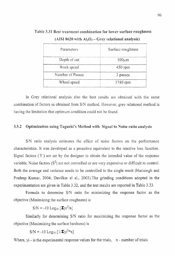
Table 3.31 Best trc;iitment com!,in:~tion for l o n e r surface roughness
(.I\ISI 8020 \\it11 A1203- G r e y retational analysis)
I
- -- -- - - - - - - -- - - - -- -- Depth O I ' C L I I I 0 0 1.i 111
t
I \+ ol h speed 150 1p1n I
Niunber 01' Passe& 3 passes I I
~ h e e E ~ e e d 1710 I-pm , .--
In Grey relational analysis also the best results are obtained with the same
combination offactors as obtained Srom SiN method. Ho\i,e~zer. grey relational method is
lia\.ing the limitation that optilnum condition coulti not b? Sound.
3.5.2 Optimization using Taguchi's S l c t l ~ o d nit11 Signal to 'Voisc rat io analysis
SIN ratio analysis estilnates the c i l c r of iioise facrol-s on the perfonnance
characteristics. It was developed as a proactive equivalent to the reactive loss function.
Signal factors (Y) are set by the designer to obtaiil tlie intended value of the response
variable. Noise factors (s') are not controlled or are very expensive or difficult to control.
Both the average and variance needs to be controlled to the single merit (Harisingh and
Pradeep Kurnar, 2004; Davillzar el al., 2003).The grinding conditions adopted in the
experimentation are given in Table 3.32, and tile test results are repolTed in Table 3.33.
Fomn~ula to determine SIN ratio for minimizing the response factor as the
oljective (Minimizing the surface roughness) is
Six = -1 0 Loglo [ ~ ~ i ' i n ]
Similarly for detenllini~lg S / N ratio for inaxirnizillg the response factor as the
objective (Maximizing the surface hardness) is
SM = -10 Loglo [ l i ~ ~ i ' * n ]
Where, yi - is the cxperime~ltal response values for tlie trials, 11 - lumber o f trials

The n\.i.i-ngc rlt;.cts oi'1naii1 I;iitor~ o n S,Y ratio oi'suri'ace I-oughness and surface
linrc!ness are g i w n in Tabii. 3.34 anti Table 3.35 fix the combination of AISI H 11 with
.l.I:0; respecti\ cl!..
Table 3.32 Grinding conditions for AISI H I I(SW ratio analysis) - - -- -- - - - - - -- - -
I
Llac!?ine used : High psecisiol: plu~lgc t1 .p~ c);iindric:tl Ciri!itiiiig bliichine of I
Model UCG 260'350 unit 500 i I
1 .-\brasi\.e wheel : AlQ; - A4hL5V . Coolant ~iscd : L\;att.r based emulsion. I I Design of expel-i~nent : Taguchi's LO ortl~ogonal array \\it11 SIN ratio analysis
Materials : AISI H 11 (Mcdium Carbon liot-ivoi.1.: stecl)
Diameter : 35 inm Lzngtli : 150 111ni
Depth of cut : 200, 300, and 400 pm. h'umbes of passes : 2,3,and4
Work speed : 56.225,and 450 ipm . Wheel speed : 1550 and 1740 lpnl
Table 3.33 Orthogonal arra? of griildii~g parameters and test results with SIN ratio (AIS1 H I 1 wi th AlzO, - SIN ratio analysis)
i- I S ho
- - 7 r - -
Dc 1 Nix
111 in N p I I
p111 ipin , I
1 - 0 1
-r--- - - - ---- -7
I sm 1 St\ Na Ra ~n urn
02 I
1 03
04
01;
06
07
08 - 09
111
9 200
300
300
300
400
400
' 4 0 0 4 5 0
I f01- fol 1
1 ip 1-11
tilal
225
56
221;
450
56
225 --
11 111 I I1 I11
tiial trial t1ia1 t~ l a l tiial j I
3 1740 0 14 0.13 0 1.5 29 30 31 1 17.1 I 39 I
x?&T-%-n%%- 0 15
0 1 8 ' 0 1 6 j
0 2 1
2
31 30
33 34 I
38 3 9
32 17 1
32 1 5 8 I
40 1 3 9 I
0 14
0 2 0
1740 0.17 0.18 0.19 39 41 40 14 9 41.6 1
3
4
2
35
3 9 4 1
3 9 9
4 1 4 )
3 v 0 2 0 0 2 0 37 7 39 38 1 4 4 4 1 2 ' 1 I I I
1740 0 13
1 5 5 0 0 . 1 4
1 7 4 0 ' 0 1 9 I
34 33 17 1 4 0 2 01.5 0 1 5 / 1
4 1740 0 I2

Table 3.34 Average effect of main factors on SIN ratio of surface roughness (AISI H I 1 with A1.03- SIN ratio analysis)
/ Average SO! value for main factors at ; I / Parameters 1 !
three levels I I I I 1 Depth of cut 1 17.37 1 15.64 15.44
1
/ Work speed 1 16.67 1 15.94 1 15.84
Level 1 I ~ e v e l 2 1 Level 3 1
I I 1
Number of Passes 14.92 16.18 17.35 1
Table 3.35 Average effect of main factors on SIN ratio of surface hardness (AISI B11 with A1203 - S/N ratio analysis)
Wheel speed
Average S I N value for main factors at
Parameters
15.39
1 three levels I
16.53
Depth of cut
Work speed
Optimum condition for surface roughness and surface hardness were found
adopting the higher the S I N ratio is better as the strategy and results are given in Table
3.36. However, the best treatment combinations out of the nine trials are third and eighth
for the low surface roughness and high surface hardness respectively.
Number of Passes
Wheel speed
Model calculation
(i) S/N ratio for minimizing the surface roughness (1 st Experimental run)
S/N = - 10 loglo {(0.16~+ 0.15~+0.17*)/3)
= 15.9063
39.38
39.93
41.07
40.52
40.22
40.2
41.04
40.5 1
39.94
40.06
39.63

( i i ) SIN ratio for maximizing the surface hardness (1st Experimental run)
Table 3.36 Optimum conditions for surface roughness and surface hardness (AISI H l l with AlzQ3- SIN ratio analysis)
Parameters / Surface roughness Surface hardness
Depth of cut 200pm 400pm
I Work speed / 56 rpm / 450 Ipm / 1 I Number of Passes / 4 passes 1 2 passes i
3.53 Optimization using Taguchi's Method with Grey relational analysis
I
Grey relational analysis combines all the responses into a single number. For this,
experimental data are first nornialized in the range between zero and one, which is also
called the grey relational generation. Grey relational coefficient is calculated from the
normalized experimental data and then g e y relational grade is computed (Lin, J.L. and
Lin, C.L., 2002). Grinding conditions adopted in the experimentation are given in Table
3.37, and the test results are reported in Table 3.38.
Wheel speed
Table 3.37 Grinding conditions for AISI T1 (Grey relational analysis)
1740 rpm
Machine used : High precision plunge type cylindrical Grinding Machine of
Model UCG 260/350 unit 500
Abrasive wheel : Alz03 - A46L5V, Coolant used : Water based emulsion
Design of experiment: Taguchi's L9 orthogonal array with Grey relational analysis
Materials : AISI T1 (High Carbon high speed steel)
Diameter : 35 mm Length : 150 mm
Depth of cut : 300,400 and 500 pm, Number of passes : 3,4 ,and 5
Work speed : 56,225, and 450 rpm, Wheel speed : 1550 and 1740 rpm

Table 3.38 Orthogonal array of grinding paranletel-s and test results
(.AlSI T1 \ \ i th .1i203 - Grey relational anal! sis) I / DC / '\J\v ' IS I R 3 in 111
I H R A I
I
1 pll, , l , ~ l l l I , 1-1x11 1 I ~ trial lriiii ~ s i s l a 1 trial 1 ~ I I 1
In the grey relational arlalysis, no]-malizing is tione and the grey I-elational
coefficient is derern~ined as per tlie follo~ving PI-ocetiuses.
Model cslculation
(i) Sn~aller the better
Smaller surface roughness is better (calculation for 1" set of data)
Nornialized value, Xii = (maxiYii - Yi,)/ (111ax,~Y~.~ -mii~,~Y ii)
X I 1=(0.24-0.17)i(0.24-0.13) = 0.63636
Grey relational coefficient <;(I<) = ( h min + 5 A ~nax)/(A ,i(k) + 5 h max)
0 (1 A min =mini 1 Xi - X i , = 0 , A max = maxi maxi Xi - Xi,/ = 1
A = 1 Xi (I -
X, " = Reference value = 1
j = Distinguishing coefficient = 0.25 (0< < c: 1 )
i(k) = (0+0.2 5" 1)/(0.36364+0.25) = 0.4074

( i i ) Largcl- the better
Lai-ger SUI-facc hardness is better (calettlation for 1"set of data)
Nai-maiizecI mluc. S, , = O',, - ~ l i i n ~ \ r ' , ~ ) , (max,Y, , -~nin,Y, , )
S ! (39-29) , (45-29) = 0.625
Cr1.t.y i-elational coef ic ient < , ( I < ) = ( A mi11 - < S max)/( A , , ,(k) + A max)
1 lnin = min, m i i ~ . I S, ' ' - - X,, = 0 . 1 m;lu = :n:ls, maxi , X, " - S,, = 1
A < , , ( I < ) = 1 Xi " - Xlil
S , " - Ret'erzi~ce \.niue = I
< = Distinguisliii~g cocfliciei~t = 0 . 2 5 (0.c < I )
< i ( l<) = (OLO.75* I ) : (0 .375~0 .25) = 0.40
Table 3.39 Grey relational analysis for surface roughness ( Xii Values)
(AISI TI with A1203 - Grey relational analysis)

Tal~ l e 3.110 Gre!. I-el;~tional an:11>-sis for surface rorigl~ncss (Xi " - Xil )Values
-- 1 I (.&IS1 TI \\.it11 .&1203 - Crcy relational analysis) 1
Table 3.41 Grey relational analysis for surface roughness - Grey relational coefficient < Values - (AISI T1 with A1203 - Gre? relational analysis)
S No 111
pm
1 1 01 j 300
02 300
Average ~ 5 Rank ,
I I Values I I
~n 3 ~n (X, " - X,, ) Values I
Iplll 1 11111 I 11 / 111
I I I t11a1 t~ la1 tl-ial I I
S No.
56 1 3 I 5 5 0 0 1 7 018 0 1 9 0.3636 I I
225 1 4 1 7 4 0 0 1 4 0.16 0 1 5 00909
1ym
Dc 1 Nw
ill 1 111 Np
0.6666
04444
Ns 111 i; Values
071421
014281

SC
m < - E
e S P 0 V)
ffi N (/I ffi -4 a

Table 3.44 Grey relational analysis fo r surface hardness -Grey relational
coefficient < \'slues - (AISI T1 \\-it11 A12Q3 - G r e y relational analysis)
i Average I
I ,i Values I 5 Rank /
Values 1 1 - -,
0 1 0 3672 ; 4 1
From the table 3 41 and 3.44. the best treatment comb~natlnl~ is found according
to the Rank for the Response factors sui-face roughness (lolver 1s better) and surface
hardness (higher 1s better) and the ~esults arz tabulated In the table -3.45.
Table 3.45 Best t rea tment combitlation for l o l ~ e r surface roughness a n d higher surface l l a r d ~ ~ e s s
(AISI T l with A1203- Grey relational analysis)
I parameters
I I
Depth of cut 1 300pm
Surface
roughness
5OOprn
Number of Passes
Wheel speed
Surface I
haidi~ess 1
Work speed 450 ipm
5 passes
1740 ipm
450 l-p~n I
3 passes
1740 ipm 1

Unlike tllc coil~~enrional surfiicu grin~liiip n.liicii ~-eiluil.es inore nuinber o f passes
to ren1oi.e the desired amount oi' t11c n.orkmaterial. the plunge cut cylindrical grinding
process can be completed in o i i l~ . a t'en,ei- passes. Because of large ciepth o f cut, specific
energy in pluilge cylindrical grinding is higher than nol.~nal grinding process. This
necessitates a special care to avoid thei-mnl darnage to the ivork piece. The production
rate achievable by grinding is often liinited by grinding temperatures and rhe resultant
hai-iniul effects on worl; piece quality. In-process energy generated being used for
strcngtllening the \i~orlz piece is considel-ed to he beneficial effect on the mechanical
properties whereas more amount of heat generation has adverse effect. So it can be
expected that by having proper control on tile grinding process. thc wear resistance o f the
\\,orl< surface can be cilhi~nced. For il~aiiy practical designs. ~vhich impose a limit on
n?asimum allowable surface roilghness. a proper operation o f many devices also,
necessities sn~ooth surfaces. The reliability of mechanical components. especially for
high strength application. often critically depends upon the sui-face and sub-sui-face
quality produced by grinding.
Analytical lllodels that explain the highly non-linear relationship with interactions
among grinding variables such as hardness value, carbon percentage, work speed, wheel
speed, depth o f cut, temperature, and surface roughness are difficult to obtain. Moreover,
at present no analytical inodels that capture the dynamics of entire grinding process
exists. Statistical models such as ~nul t i response graph/ S-N ratio model i Liner regression
iGray relational requires assumptioils about the parametric and functional nature of the
factors, which inay or nlay not be true. Also, this reduced linear o r lower power inodel is
not enough to describe the coinplicated input / o~ltput relations i11 the grinding process.
-4rtificial intelligent Techniques such as neural network and expert systenls have
been increasingly used to successfully inodel complex process behaviour in areas where
analytical inodels are unavailable or difficult to implement. The use of neural network is
motivated because of their accon~modation of non-linearities, interactions and nlultiple

1,ariabIes. Neural networks are also tolerant of noise data anci respond to the operating
cilndition fairly quiclily so that the hardi\.are part of i t can be integrated with the
system/machine for real rinis control. Neural net\vorks do not ~-equire such assumptions,
\\-Iiich are esseiitial for tlie analysis using other con~.entional models or tools. Neural
nt.tn.o~.k models are data driven nloclels. The neural nt.ti\.oi.ks have strong abilities to
learn and self organizc infol-mation ant! need only a specific requireme~lt and prior
different set of assunlptions for modeling (\Jijayaraha\.an er al.. 2003). These advantages
hate attracted much interest in combini~-ig ANN lvith Taguchi's Design of Experiments.
The objecti1;e of this study is to model and forecast the grinding process by
applying Back Propagation Algorithnl (BPA). Tlie experimental data using Taguchi's
design of experiment technique is used in the training of the BP network. The .ANN
results are compared n.ith the experimental results.
3.6.1 Neural Ketwork used
In the present ivol-k, a multilayer perceptrons with each layer consisting of
number of computing neurons l i a t t been used. The algorithm used in this \vori< is BPA.
The BPA uses the steepest descenl method lo reach a global minimurn. The number of
layers and number of nodes in the hidden layers are decided. Tlie connections between
nodes are initialized n;ith ral~dolil weights. A pattern from tlie training set is presented in
the input layer of the network and the error at the output layer is calculated. The ei-ror is
propagated backwards towards the input layer and the weights are updated. This
procedure is repeated for all the training patterns. At the end o f each iteration. test
pattei-ns are presented to ANN and the classification performance o f ANN is evaluated.
Further training of AKN is continued till the desired classification p e r f o ~ l l ~ a ~ ~ c e is
reached. The weights "MT" and the threshold values "0" are adjusted until the e n o r
comes within the limit (Fengguo Cao and Qinjian Zang, 2004).The steps involved in
training ANN by using BPA are.

Step I The \\,eights ancl tl?resiioltis arc ra~~dorn ly initializeti bctureen layers by impoiTing
the Esperimzniai input arlti output to the k1.ATLhB.
Step 2 The inpui oi'a piirtcrli is pl.csctltcd to tlie input Inyzi- :untl the outputs o f t h e
neuron a!-r computcd as l i j i l ~ \ \ ' ~ :
The ac~i\.ation ti~nction ';I' ~isccl 1ie1.z is the PURELIN i i~~?ct ioi l and is given by:
a = w " p - i b
between the iiipuis. iiitliirn and o ~ ~ t p ~ i t l a y r s .
Where. \v is tile \vcigi~t. p is thc input neuron anti b is tile bias values.
Step 3
The training of ANN is done \vitli number of itesatiolis.
Step 4
The ell-or pattern is calculated.
Step 5
The en-or is minimized by ~.aryiiig tile ANN configuration.
Step 6
For each training pattern. steps 3 and 4 are repeated tiil the goal is reaci2ed.
Step 7
The itera~ion process contii~ues until the desired goal is rcached.
When the .4KN training is over, the network can predict tlie surface roughness!
surface hardness using the feed forward mechanism. Tbe ,ANN model of configuration
4-9-9-2 used in this study for training and testing the data is sllown in figure 3.3. The NN
architecture is of Back Propagation Algorith~n with Feed F o ~ w a r d type composed of four
layers .There are four neurons in the input layer for the four input variables naintly depth
of cut, number of passes, work speed and wheel speed. I11 tlie output layer, one neuron is
used for surface roughness (R,) and the other one for surface hardness (HRA). T w o
hidden layers with nine (9) nodes each are selected.
At the main paif of the network architecture, the number of hidden layers ,nodes
is the key problem to be solved. More hidden layers and nodes will lead to long training
time, whereas less hidden layers and nodes may deteriorate the training effect. I n many

cases. the detei?~~inatioi; oS the !:urnbi.~ of hidden layers anti 11odes depends heavily on the
r s p a i e n c e or expesims~:ts. Tilo Rcnson lhs selecting TWO hidden layers in th is
co~itiguration is to reclucr ossos ant! time factor also. The .4KN is trained wit11 different
number of nodes in the llidden i~iyer. Tile val.>,ing plot o f the training time and t ra in ing
ssroi. \.cssus the number of hiddtr: 1;odcs is si:o\\.ii in figure 3.4. I t is seen t h a t if the
rruiniiig time a~ltI 11,aining errol- art. co!~sitic:-i.ti simuirant.ousiy the optimal nu l l lbz r of
hidtien nodes shoult! b s nine (0).
Figure 3.3 A Typical \lultilayered Feed forward back Propaga t ion 1 N Model of co~ifiguration 4-9-9-2
0 3 6 9 1 2 \ o . o f V o d e s i n H ~ d e e n l a y e r s
Figure 3.4 Relationship between Training time a n d Training e r r o r and the Number of hidden nodes in the hidden layers

3.7 Results and discussion
The productivity. accuracy. and cost of grinding process depend to a considerable
extent on the correct choice of'gi-inding wheel, as the ad\.nntages of a good machine and
optirnunl-grinding conditions can be lost by operating then1 under unsuitable/
unfa\,ourable grinding wheel.
A variety of Iiigh precision machinvs ha\^ been in use and new surface generation
n ~ ~ ~ c h i n e s are constantly being de\,eIoprd to achii.\,c estl-emely close geometric tolerances
or to improve surface tinish. The objccti\.e of all high preoisii~n grinding machines is to
acliieve geometrically precise co~npo~icn ts or surlkce of' conirolled texture or surface
finish.
Rased 011 the results o f tlie pi-eliminary eupesiments conducted, plunge type
cylindrical grinding machine \v~tll Al? 0; is selected and used for all the grinding tests
involved in this work.
Not only the machine and cutting tool, but the operational factors are also having
a greater influence on the quality and productivity impro\!ernent. Quality and productivity
iinprovement is most effective when it is an integral part of the product and process
developmellt cycle. The introduction of proper design of experiment at the earliest stage
of development cycle where new products are designed , existing products design
iniproved, and nianufacturiii process optinlized is often key to overall product success.
In order to coilduct study on this. a comparative study between Taguchi's DOE and
Factorial DOE is made. The test results obtained from both of these methods are listed in
table 3.8 and 3.9.
Both the case studies show that depth of cut and number of passes are having
more influence i.e.: 31.40% and 38.72% respectively under Taguchi's method and
29.07% and 35.83% respectively under Factorial method on surface roughness of the
workpiece. Optimal conditions are directly obtained from Taguchl's method. whereas.
Factorial method gives a regression model to predict the surface roughness for ally input

\aiue. Factorial l l ~ t . t h ~ d is not a simple analysis. But Taguchi's inethod is a si~iil?le
method of DOE. efficient. systematic. small number of tests and large number o f
info]-mation. Hence. Taguchi's n:ctliod of DOE is followed for all the grinding tl-ials
involved in this work.
The traditional factorial espe~~itnenral tiesign pl.oct'du~.c ti)ci~ses on the average
product or process pel-hi-manct. cllat-acreristics. But the Tagucl~i 's metl~od concentrates
on the efl'ect of variation on tllc prociucl or process quality chor;lcttrristics rather than on
its averages (Phadkc. M. S.. 1989; Rosb ..[01in. P, 1980). T11;1[ is. tlie Taguchi's approach
makes the product or proccss perfhrmance inseiisiti\,e (robust) to variations in
uncontrolled (or) noise 1.actors. To achieve the required cluality in a specific situation.
operating parameters are ofien detel-mined with the aid of grintiing tests. I f nlorc nui~iber
of parameters are there, the conventional testing methods are time consu~ning and
expensive. Here lies the importance of the Taguchi's method for the design o f
experiment.
AISI 8620, H l I , and T 1 carbon steels are subjected for grinding test. The surface
roughness of the ground pieces which is one of the n u i n quality requirements and the
surface hardness which is the secondary response variable are selected as quality
characteristics for the study and their results are presented in tables 3.20, 3.33 and 3.38.
The operating conditions such a s Depth of cut. Nulnber of passes. Wheel speed and
Workspeed which are generally controllable in any grinding situation are selected as
factors for study. Three levels having equal spacing within the operating range of the
iilachine are selected for each of the factors. By selecting three levels, the nonlinearity
effects could be studied. The data obtained are analyzed by three different optimization
methods for different nlaterials and details are given below.
(i) AISI 8620 -- Response graph method and vei-lfication with SIX ratio
method and Grey relational method.
(ii) AISI Hl 1 -- Signal to Noise ratio method.
(iii) AISI T1 -- Grey relational method.

Analysis oi ' \ariance ( .INO\''-\) is tione for XIS1 33 10. 1330. 1040, and 8620. The
.4kOVA results (Tables 3.6. 3.1 i . 3.17 and 3.23) indicate that depth o f cut is having
more influence on the surface roughness, surface hartlness. If the depth o f cut is low the
surface finish is good. Howe\,er. if the depth of cut is r;loi-e the hardness improve (Table
3.21).
Figure 3 . I and 3.2 s h o ~ i . the response graph obtained for the material AISI 8620.
They show that a nlodernte feed spceti is reci~~il-cd to attain n good si~rface finish grounded
components with liigii su1.111ce 1;al.dncss. For the material AISI 8670 .Response graph
inethod. Signal to Noise ratio metl~od and Grey relational a11pl.oacii have given the same
optimal i best treatment combination results (Tables 3.21, 3.27. and 3.3 1 j.
Similarly. Signal to Noise ratio method and Grey relational approach h a w given
the same optinla1 parameters level I best treatment conlbination results for the materials
AIS1 H 11 and T I(Tab1es 3.36, and 3.45).
For all the optiillu~n results obtained. the confirmation trials are carried out in
grinding machine. The confimlation of experiment sho\\ls that tlie experimental
observations (surface roughness and surface hardness) and estimated results are very
close and the percentage deviation is in tlie accepted level of 2-3 percentages.
The optinlization studies on different nlaterials at different conditions by different
techniques reveal that the depth of cut and nulnber of passes are having greater effect on
surface integrity of the workpiece. In industries mostly. in order to remove the blackened
surfaces of surface hardened components, finish grinding is done. During this material
removal, the hardness of the hardened components decreases. In order to avoid this
reduction in hardness level and to have less grinding cycle time, t l ~ e maximum nletal
removal depth to be kept, as far as possible, as the minimal one.
Nowadays, for high volume o f metal removal also grinding process is used. In
such a case, the intense heat generated in grinding due to relatively high fi-ictional effect

impairs xvorl;piecc ciuality 1,. incii~ciiig tliermnl damage. Therefore, cooiirig and
lubrication play n tlecisi\.e role i l l grinding. E1,i.n thougii. many limitations 11ax.e been
observed in the usage of coolnnrs, liquid coolants in flood form have been the
choice to deal wit11 the thermal damages.
Simple. quick and economic parameters selection methods are very much needed
by the industry. In the present \yolk. it is accomplished through integrating Taguchi's
DOE with ANN.
With nine (9) data sets for AISI 8620 ~iiaterial (Table 3.20) thz YN is instructed to
SUII for 5000 iterations with tile prograni developed in MATLAB. The average percentage
training error is 8.22 ?/o and 3.87% i'or Ra and HR.4 I-espectiveiy (Table 3.46, figure
3.jand figure 3.6). As can be see11 from the figures 3.5 and 3.6 the training of the model
is successfully accomplished. The nlodel is x'ery closc to the actual data and is able to
follotv the trend. The value of the ANN trials and experimental trials correspond closely.
Table 3.46 Esperimental results Vs ANN predicted results with training error at 5000 iterations ai
Experilllent al -
I 1
9
Expt. ANN / Expt. AKIi
0.16
order values
I % elms , I, % ell-or values i i values values !
i
0.1534
Average error
4 125 34 35.3393 3 9391 18 I
8.223354 Average error 3.876667

Concluding remarks
, Figure 3.5 Experimental Surface Roughness Figure 3.6 Elperimental Surface Hardness 1 1
O Depth of cut is having inore influence on the surface integrity of the grounded
parts.
~ a l u e s Vs ANS predicted Surface Roughness L alues
I
Q A1203 is better suiled for grinding carbon steels than SIC since S i c gives a pool
surface finish.
~ a l u c s Vs ANN predicted Surface Hardness Yalues
*:* Optimization of the process parameters in cylindrical grinding process was done
by integrating Taguchi's parameter design and AUK\'. This approach has been
found to be very effecrive in optimization.