Chapter 3

The autocovariance function of a

linear time series

Objectives

• Be able to determine the rate of decay of an ARMA time series.

• Be able ‘solve’ the autocovariance structure of an AR process.

• Understand what partial correlation is and how this may be useful in determining the order

of an AR model.

• Understand why autocovariance is ‘blind’ to processes which are non-causal. But the higher

order cumulants are not ‘blind’ to causality.

3.1 The autocovariance function

The autocovariance function (ACF) is defined as the sequence of covariances of a stationary process.

That is suppose that {Xt} is a stationary process with mean zero, then {c(k) : k 2 Z} is the ACF

of {Xt} where c(k) = E(X0

Xk). Clearly di↵erent time series give rise to di↵erent features in the

ACF. We will explore some of these features below.

Before investigating the structure of ARMA processes we state a general result connecting linear

time series and the summability of the autocovariance function.

83

Lemma 3.1.1 Suppose the stationary time series Xt satisfies the linear representationP1

j=�1 j"t�j.

The covariance is c(r) =P1

j=�1 j j+r.

(i) IfP1

j=1 | j | < 1, thenP

k |c(k)| < 1.

(ii) IfP1

j=1 |j j | < 1, thenP

k |k · c(k)| < 1.

(iii) IfP1

j=1 | j |2 < 1, then we cannot say anything about summability of the covariance.

PROOF. It is straightforward to show that

c(k) = var["t]X

j

j j�k.

Using this result, it is easy to see thatP

k |c(k)| P

k

P

j | j | · | j�k|, thusP

k |c(k)| < 1, which

proves (i).

The proof of (ii) is similar. To prove (iii), we observe thatP

j | j |2 < 1 is a weaker condition

thenP

j | j | < 1 (for example the sequence j = |j|�1 satisfies the former condition but not the

latter). Thus based on the condition we cannot say anything about summability of the covariances.

⇤

First we consider a general result on the covariance of a causal ARMA process (always to obtain

the covariance we use the MA(1) expansion - you will see why below).

3.1.1 The rate of decay of the autocovariance of an ARMA process

We evaluate the covariance of an ARMA process using its MA(1) representation. Let us suppose

that {Xt} is a causal ARMA process, then it has the representation in (2.21) (where the roots of

�(z) have absolute value greater than 1 + �). Using (2.21) and the independence of {"t} we have

cov(Xt, X⌧ ) = cov(1X

j1

=0

aj1

"t�j1

,1X

j2

=0

aj2

"⌧�j2

)

=1X

j=0

aj1

aj2

cov("t�j , "⌧�j) =1X

j=0

ajaj+|t�⌧ |var("t) (3.1)

(here we see the beauty of the MA(1) expansion). Using (2.22) we have

|cov(Xt, X⌧ )| var("t)C2

⇢

1X

j=0

⇢j⇢j+|t�⌧ | C2

⇢⇢|t�⌧ |

1X

j=0

⇢2j =⇢|t�⌧ |

1� ⇢2, (3.2)

84

for any 1/(1 + �) < ⇢ < 1.

The above bound is useful, it tells us that the ACF of an ARMA process decays exponentially

fast. In other words, there is very little memory in an ARMA process. However, it is not very

enlightening about features within the process. In the following we obtain an explicit expression for

the ACF of an autoregressive process. So far we have used the characteristic polynomial associated

with an AR process to determine whether it was causal. Now we show that the roots of the

characteristic polynomial also give information about the ACF and what a ‘typical’ realisation of

a autoregressive process could look like.

3.1.2 The autocovariance of an autoregressive process

Let us consider the zero mean AR(p) process {Xt} where

Xt =p

X

j=1

�jXt�j + "t. (3.3)

From now onwards we will assume that {Xt} is causal (the roots of �(z) lie outside the unit circle).

Given that {Xt} is causal we can derive a recursion for the covariances. It can be shown that

multipying both sides of the above equation by Xt�k (k 0) and taking expectations, gives the

equation

E(XtXt�k) =p

X

j=1

�jE(Xt�jXt�k) + E("tXt�k)| {z }

=0

=p

X

j=1

�jE(Xt�jXt�k). (3.4)

It is worth mentioning that if the process were not causal this equation would not hold, since "t

and Xt�k are not necessarily independent. These are the Yule-Walker equations, we will discuss

them in detail when we consider estimation. For now letting c(k) = E(X0

Xk) and using the above

we see that the autocovariance satisfies the homogenuous di↵erence equation

c(k)�p

X

j=1

�jc(k � j) = 0, (3.5)

for k � 0. In other words, the autocovariance function of {Xt} is the solution of this di↵erence

equation. The study of di↵erence equations is a entire field of research, however we will now scratch

the surface to obtain a solution for (3.5). Solving (3.5) is very similar to solving homogenuous

di↵erential equations, which some of you may be familar with (do not worry if you are not).

85

Recall the characteristic polynomial of the AR process �(z) = 1 � Ppj=1

�jzj = 0, which has

the roots �1

, . . . ,�p. In Section 2.3.4 we used the roots of the characteristic equation to find the

stationary solution of the AR process. In this section we use the roots characteristic to obtain the

solution (3.5). It can be shown if the roots are distinct (the roots are all di↵erent) the solution of

(3.5) is

c(k) =p

X

j=1

Cj��kj , (3.6)

where the constants {Cj} are chosen depending on the initial values {c(k) : 1 k p} and are

such that they ensure that c(k) is real (recalling that �j) can be complex.

The simplest way to prove (3.6) is to use a plugin method. Plugging c(k) =Pp

j=1

Cj��kj into

(3.5) gives

c(k)�p

X

j=1

�jc(k � j) =p

X

j=1

Cj

✓

��kj �

pX

i=1

�i��(k�i)j

◆

=p

X

j=1

Cj��kj

✓

1�p

X

i=1

�i�ij

◆

| {z }

�(�i

)

= 0.

In the case that the roots of �(z) are not distinct, let the roots be �1

, . . . ,�s with multiplicity

m1

, . . . ,ms (Ps

k=1

mk = p). In this case the solution is

c(k) =s

X

j=1

��kj Pm

j

(k), (3.7)

where Pmj

(k) is mjth order polynomial and the coe�cients {Cj} are now ‘hidden’ in Pmj

(k). We

now study the covariance in greater details and see what it tells us about a realisation. As a

motivation consider the following example.

Example 3.1.1 Consider the AR(2) process

Xt = 1.5Xt�1

� 0.75Xt�2

+ "t, (3.8)

where {"t} are iid random variables with mean zero and variance one. The corresponding charac-

teristic polynomial is 1 � 1.5z + 0, 75z2, which has roots 1 ± i3�1/2 =p

4/3 exp(i⇡/6). Using the

86

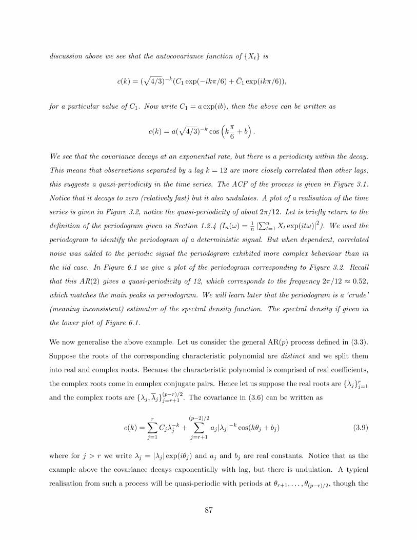
discussion above we see that the autocovariance function of {Xt} is

c(k) = (p

4/3)�k(C1

exp(�ik⇡/6) + C1

exp(ik⇡/6)),

for a particular value of C1

. Now write C1

= a exp(ib), then the above can be written as

c(k) = a(p

4/3)�k cos⇣

k⇡

6+ b

⌘

.

We see that the covariance decays at an exponential rate, but there is a periodicity within the decay.

This means that observations separated by a lag k = 12 are more closely correlated than other lags,

this suggests a quasi-periodicity in the time series. The ACF of the process is given in Figure 3.1.

Notice that it decays to zero (relatively fast) but it also undulates. A plot of a realisation of the time

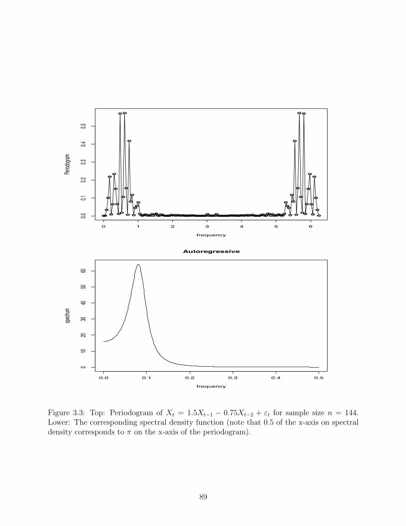
series is given in Figure 3.2, notice the quasi-periodicity of about 2⇡/12. Let is briefly return to the

definition of the periodogram given in Section 1.2.4 (In(!) =1

n |Pnt=1

Xt exp(it!)|2). We used the

periodogram to identify the periodogram of a deterministic signal. But when dependent, correlated

noise was added to the periodic signal the periodogram exhibited more complex behaviour than in

the iid case. In Figure 6.1 we give a plot of the periodogram corresponding to Figure 3.2. Recall

that this AR(2) gives a quasi-periodicity of 12, which corresponds to the frequency 2⇡/12 ⇡ 0.52,

which matches the main peaks in periodogram. We will learn later that the periodogram is a ‘crude’

(meaning inconsistent) estimator of the spectral density function. The spectral density if given in

the lower plot of Figure 6.1.

We now generalise the above example. Let us consider the general AR(p) process defined in (3.3).

Suppose the roots of the corresponding characteristic polynomial are distinct and we split them

into real and complex roots. Because the characteristic polynomial is comprised of real coe�cients,

the complex roots come in complex conjugate pairs. Hence let us suppose the real roots are {�j}rj=1

and the complex roots are {�j ,�j}(p�r)/2j=r+1

. The covariance in (3.6) can be written as

c(k) =r

X

j=1

Cj��kj +

(p�2)/2X

j=r+1

aj |�j |�k cos(k✓j + bj) (3.9)

where for j > r we write �j = |�j | exp(i✓j) and aj and bj are real constants. Notice that as the

example above the covariance decays exponentially with lag, but there is undulation. A typical

realisation from such a process will be quasi-periodic with periods at ✓r+1

, . . . , ✓(p�r)/2, though the

87

0 10 20 30 40 50

−0.4

−0.2

0.00.2

0.40.6

0.81.0

lag

acf

Figure 3.1: The ACF of the time series Xt = 1.5Xt�1

� 0.75Xt�2

+ "t

Time

ar2

−4−2

02

46

0 24 48 72 96 120 144

Figure 3.2: The a simulation of the time series Xt = 1.5Xt�1

� 0.75Xt�2

+ "t

88

●●

●

●

●

●

●

●

●

●

●

●

●

●

●

●

●

●

●

●

●

●●

●

●●●●

●●●●

●●●●●●●●●●●●●●●●●●●●●●●●●●●●●●●●●●●●●

●●●●●●

●●●●●●●●●●●●●●●●●●●●●●●●●●●●●●●

●●●●●●●●●●

●●●●●

●

●●

●

●

●

●

●

●

●

●

●

●

●

●

●

●

●

●

●

●

●

●

0 1 2 3 4 5 6

0.00.1

0.20.3

0.40.5

frequency

Periodo

gram

0.0 0.1 0.2 0.3 0.4 0.5

010

2030

4050

60

frequency

spectru

m

Autoregressive

Figure 3.3: Top: Periodogram of Xt = 1.5Xt�1

� 0.75Xt�2

+ "t for sample size n = 144.Lower: The corresponding spectral density function (note that 0.5 of the x-axis on spectraldensity corresponds to ⇡ on the x-axis of the periodogram).

89

magnitude of each period will vary.

An interesting discussion on covariances of an AR process and realisation of an AR process is

given in Shumway and Sto↵er (2006), Chapter 3.3 (it uses the example above). A discussion of

di↵erence equations is also given in Brockwell and Davis (1998), Sections 3.3 and 3.6 and Fuller

(1995), Section 2.4.

Example 3.1.2 (Autocovariance of an AR(2)) Let us suppose that Xt satisfies the model Xt =

(a+ b)Xt�1

� abXt�2

+ "t. We have shown that if |a| < 1 and |b| < 1, then it has the solution

Xt =1

b� a

�

1X

j=0

�

bj+1 � aj+1)"t�j

�

.

By writing a ‘timeline’ it is straightfoward to show that for r > 1

cov(Xt, Xt�r) =1X

j=0

(bj+1 � aj+1)(bj+1+r � aj+1+r).

Example 3.1.3 The autocorrelation of a causal and noncausal time series Let us consider the two

AR(1) processes considered in Section 2.3.2. We recall that the model

Xt = 0.5Xt�1

+ "t

has the stationary causal solution

Xt =1X

j=0

0.5j"t�j .

Assuming the innovations has variance one, the ACF of Xt is

cX(0) =1

1� 0.52cX(k) =

0.5|k|

1� 0.52

On the other hand the model

Yt = 2Yt�1

+ "t

90

has the noncausal stationary solution

Yt = �1X

j=0

(0.5)j+1"t+j+1

.

Thus process has the ACF

cY (0) =0.52

1� 0.52cX(k) =

0.52+|k|

1� 0.52.

Thus we observe that except for a factor (0.5)2 both models has an identical autocovariance function.

Indeed their autocorrelation function would be same. Furthermore, by letting the innovation of Xt

have standard deviation 0.5, both time series would have the same autocovariance function.

Therefore, we observe an interesting feature, that the non-causal time series has the same

correlation structure of a causal time series. In Section 3.3 that for every non-causal time series

there exists a causal time series with the same autocovariance function. Therefore autocorrelation

is ‘blind’ to non-causality.

Exercise 3.1 Recall the AR(2) models considered in Exercise 2.4. Now we want to derive their

ACF functions.

(i) (a) Obtain the ACF corresponding to

Xt =7

3Xt�1

� 2

3Xt�2

+ "t,

where {"t} are iid random variables with mean zero and variance �2.

(b) Obtain the ACF corresponding to

Xt =4⇥p

3

5Xt�1

� 42

52Xt�2

+ "t,

where {"t} are iid random variables with mean zero and variance �2.

(c) Obtain the ACF corresponding to

Xt = Xt�1

� 4Xt�2

+ "t,

where {"t} are iid random variables with mean zero and variance �2.

91

(ii) For all these models plot the true ACF in R. You will need to use the function ARMAacf.

BEWARE of the ACF it gives for non-causal solutions. Find a method of plotting a causal

solution in the non-causal case.

Exercise 3.2 In Exercise 2.5 you constructed a causal AR(2) process with period 17.

Load Shumway and Sto↵er’s package astsa into R (use the command install.packages("astsa")

and then library("astsa").

Use the command arma.spec to make a plot of the corresponding spectral density function. How

does your periodogram compare with the ‘true’ spectral density function?

R code

We use the code given in Shumway and Sto↵er (2006), page 101 to make Figures 3.1 and 3.2.

To make Figure 3.1:

acf = ARMAacf(ar=c(1.5,-0.75),ma=0,50)

plot(acf,type="h",xlab="lag")

abline(h=0)

To make Figures 3.2 and 6.1:

set.seed(5)

ar2 <- arima.sim(list(order=c(2,0,0), ar = c(1.5, -0.75)), n=144)

plot.ts(ar2, axes=F); box(); axis(2)

axis(1,seq(0,144,24))

abline(v=seq(0,144,12),lty="dotted")

Periodogram <- abs(fft(ar2)/144)**2

frequency = 2*pi*c(0:143)/144

plot(frequency, Periodogram,type="o")

library("astsa")

arma.spec( ar = c(1.5, -0.75), log = "no", main = "Autoregressive")

92

3.1.3 The autocovariance of a moving average process

Suppose that {Xt} satisfies

Xt = "t +q

X

j=1

✓j"t�j .

The covariance is

cov(Xt, Xt�k) =

8

<

:

Ppi=0

✓i✓i�k k = �q, . . . , q

0 otherwise

where ✓0

= 1 and ✓i = 0 for i < 0 and i � q. Therefore we see that there is no correlation when

the lag between Xt and Xt�k is greater than q.

3.1.4 The autocovariance of an autoregressive moving average pro-

cess

We see from the above that an MA(q) model is only really suitable when we believe that there

is no correlaton between two random variables separated by more than a certain distance. Often

autoregressive models are fitted. However in several applications we find that autoregressive models

of a very high order are needed to fit the data. If a very ‘long’ autoregressive model is required

a more suitable model may be the autoregressive moving average process. It has several of the

properties of an autoregressive process, but can be more parsimonuous than a ‘long’ autoregressive

process. In this section we consider the ACF of an ARMA process.

Let us suppose that the causal time series {Xt} satisfies the equations

Xt �p

X

i=1

�iXt�i = "t +q

X

j=1

✓j"t�j .

We now define a recursion for ACF, which is similar to the ACF recursion for AR processes. Let

us suppose that the lag k is such that k > q, then it can be shown that the autocovariance function

of the ARMA process satisfies

E(XtXt�k)�p

X

i=1

�iE(Xt�iXt�k) = 0

93

On the other hand, if k q, then we have

E(XtXt�k)�p

X

i=1

�iE(Xt�iXt�k) =q

X

j=1

✓jE("t�jXt�k) =q

X

j=k

✓jE("t�jXt�k).

We recall that Xt has the MA(1) representation Xt =P1

j=0

aj"t�j (see (2.21)), therefore for

k j q we have E("t�jXt�k) = aj�kvar("t) (where a(z) = ✓(z)�(z)�1). Altogether the above

gives the di↵erence equations

c(k)�p

X

i=1

�ic(k � i) = var("t)q

X

j=k

✓jaj�k for 1 k q (3.10)

c(k)�p

X

i=1

�ic(k � i) = 0, for k > q,

where c(k) = E(X0

Xk). (3.10) is homogenuous di↵erence equation, then it can be shown that the

solution is

c(k) =s

X

j=1

��kj Pm

j

(k),

where �1

, . . . ,�s with multiplicity m1

, . . . ,ms (P

k ms = p) are the roots of the characteristic

polynomial 1�Ppj=1

�jzj . Observe the similarity to the autocovariance function of the AR process

(see (3.7)). The coe�cients in the polynomials Pmj

are determined by the initial condition given

in (3.10).

You can also look at Brockwell and Davis (1998), Chapter 3.3 and Shumway and Sto↵er (2006),

Chapter 3.4.

3.2 The partial covariance and correlation of a time

series

We see that by using the autocovariance function we are able to identify the order of an MA(q)

process: when the covariance lag is greater than q the covariance is zero. However the same is

not true for AR(p) processes. The autocovariances do not enlighten us on the order p. However

a variant of the autocovariance, called the partial autocovariance is quite informative about order

of AR(p). We start by reviewing the partial autocovariance, and it’s relationship to the inverse

94

variance/covariance matrix (often called the precision matrix).

3.2.1 A review of multivariate analysis

A cute little expression for the prediction error

In the following section we define the notion of partial correlation. However, we start with a nice

(well known) expression from linear regression which expresses the prediction errors in terms of

determinants matrices.

Suppose (Y,X), where X = (X1

, . . . , Xp) is a random vector. The best linear predictor of Y

given X is given by

bY =p

X

j=1

�jXj

where � = ⌃�1

XX⌃XY , with � = (�1

, . . . ,�p) and ⌃XX = var(X), ⌃XY = cov[X, Y ]. It is well know

that the prediction error is

E[Y � bY ]2 = �Y � ⌃Y X⌃�1

XX⌃XY . (3.11)

with �Y = var[Y ]. Let

⌃ =

0

@

var[Y ] ⌃Y X

⌃XY ⌃XX

1

A . (3.12)

We show below that that prediction error can be rewritten as

E[Y � bY ]2 = �Y � ⌃Y X⌃�1

XX⌃XY =det(⌃)

det(⌃XX). (3.13)

To prove this result we use (thank you for correcting this!)

det

0

@

A B

C D

1

A = det(D) det�

A�BD�1C�

. (3.14)

95

Applying this to (3.14) gives

det(⌃) = det(⌃XX)�

�Y � ⌃Y X⌃�1

XX⌃XY

�

) det(⌃) = det(⌃XX)E[Y � bY ]2, (3.15)

thus giving (3.13).

The above result leads to two more useful relations, which we now summarize. The first uses

the following result on inverse of block matrices

0

@

A B

C D

1

A

�1

(3.16)

=

0

@

A�1 +A�1BP�1CA�1 �A�1BP�1

�P�1CA�1 P�1

1

A =

0

@

P�1

1

�P�1

1

BD�1

�D�1CP�1

1

D�1 +D�1CP�1

1

BD�1

1

A ,

where P = (D � CA�1B) and P1

= (A � BD�1C). Now comparing the above with (3.12) and

(3.11) we see that

�

⌃�1

�

11

=1

�Y � ⌃Y X⌃�1

XX⌃XY

=1

E[Y � bY ]2.

In other words, the inverse of the top left hand side of the matrix ⌃ gives the inverse mean squared

error of Y given X. Furthermore, by using (3.13) this implies that

�

⌃�1

�

11

=1

E[Y � bY ]2=

det(⌃XX)

det(⌃). (3.17)

Partial correlation

Suppose X = (X1

, . . . , Xd) is a zero mean random vector (we impose the zero mean condition to

simplify notation and it’s not necessary). The partial correlation is the covariance between Xi and

Xj , conditioned on the other elements in the vector. In other words, the covariance between the

residuals of Xi conditioned on X�(ij) (the vector not containing Xi and Xj) and the residual of Xj

conditioned on X�(ij). That is the partial covariance between Xi and Xj given X�(ij) is defined

96

as

cov�

Xi � var[X�(ij)]�1E[X�(ij)Xi]X�(ij), Xj � var[X�(ij)]

�1E[X�(ij)Xj ]X�(ij)

�

= cov[XiXj ]� E[X�(ij)Xi]0var[X�(ij)]

�1E[X�(ij)Xj ].

Taking the above argument further, the variance/covariance matrix of the residual of Xij =

(Xi, Xj)0 given X�(ij) is defined as

var�

Xij � E[Xij ⌦X�(ij)]0var[X�(ij)]

�1X�(ij)

�

= ⌃ij � c0ij⌃�1

�(ij)cij (3.18)

where ⌃ij = var(Xij), cij = E(Xij ⌦ X�(ij)) (=cov(Xij ,X�(ij))) and ⌃�(ij) = var(X�(ij))

(⌦ denotes the tensor product). Let sij denote the (i, j)th element of the (2 ⇥ 2) matrix ⌃ij �c0ij⌃

�1

�(ij)cij . The partial correlation between Xi and Xj given X�(ij) is

⇢ij =s12p

s11

s22

,

observing that

(i) s12

is the partial covariance between Xi and Xj .

(ii) s11

= E(Xi �P

k 6=i,j �i,kXk)2 (where �i,k are the coe�cients of the best linear predictor of

Xi given {Xk; k 6= i, j}).

(ii) s22

= E(Xj �P

k 6=i,j �j,kXk)2 (where �j,k are the coe�cients of the best linear predictor of

Xj given {Xk; k 6= i, j}).

In the following section we relate partial correlation to the inverse of the variance/covariance

matrix (often called the precision matrix).

The precision matrix and its properties

Let us suppose that X = (X1

, . . . , Xd) is a zero mean random vector with variance ⌃. The (i, j)th

element of ⌃ the covariance cov(Xi, Xj) = ⌃ij . Here we consider the inverse of ⌃, and what

information the (i, j)th of the inverse tells us about the correlation between Xi and Xj . Let ⌃ij

denote the (i, j)th element of ⌃�1. We will show that with appropriate standardisation, ⌃ij is the

97

negative partial correlation between Xi and Xj . More precisely,

⌃ij

p⌃ii⌃jj

= �⇢ij . (3.19)

The proof uses the inverse of block matrices. To simplify the notation, we will focus on the (1, 2)th

element of ⌃ and ⌃�1 (which concerns the correlation between X1

and X2

).

Remark 3.2.1 Remember the reason we can always focus on the top two elements of X is because

we can always use a permutation matrix to permute the Xi and Xj such that they become the top

two elements. Since the inverse of the permutation matrix is simply its transpose everything still

holds.

LetX1,2 = (X

1

, X2

)0,X�(1,2) = (X3

, . . . , Xd)0, ⌃�(1,2) = var(X�(1,2)), c1,2 = cov(X

(1,2),X�(1,2))

and ⌃1,2 = var(X

1,2). Using this notation it is clear that

var(X) = ⌃ =

0

@

⌃1,2 c

1,2

c01,2 ⌃�(1,2)

1

A . (3.20)

By using (3.16) we have

⌃�1 =

0

@

P�1 �P�1c01,2⌃

�1

�(1,2)

�⌃�1

�(1,2)c1,2P�1 P�1 + ⌃�1

�(1,2)c1,2P�1c0

1,2⌃�1

�(1,2)

1

A , (3.21)

where P = (⌃1,2 � c0

1,2⌃�1

�(1,2)c1,2). Comparing P with (3.18), we see that P is the 2⇥ 2 variance/-

covariance matrix of the residuals of X(1,2) conditioned on X�(1,2). Thus the partial correlation

between X1

and X2

is

⇢1,2 =

P1,2

p

P1,1P2,2

(3.22)

where Pij denotes the elements of the matrix P . Inverting P (since it is a two by two matrix), we

see that

P�1 =1

P1,1P2,2 � P 2

1,2

0

@

P2,2 �P

1,2

�P1,2 P

11

1

A . (3.23)

98

Thus, by comparing (3.21) and (3.23) and by the definition of partial correlation given in (3.22) we

have

P�1

1,2 = �⇢1,2.

Let ⌃ij denote the (i, j)th element of ⌃�1. Thus we have shown (3.19):

⇢ij = � ⌃ij

p⌃ii⌃jj

.

In other words, the (i, j)th element of ⌃�1 divided by the square root of it’s diagonal gives negative

partial correlation. Therefore, if the partial correlation between Xi and Xj given Xij is zero, then

⌃i,j = 0.

The precision matrix, ⌃�1, contains many other hidden treasures. For example, the coe�cients

of ⌃�1 convey information about the best linear predictorXi givenX�i = (X1

, . . . , Xi�1

, Xi+1

, . . . , Xd)

(all elements of X except Xi). Let

Xi =X

j 6=i

�i,jXj + "i,

where {�i,j} are the coe�cients of the best linear predictor. Then it can be shown that

�i,j = �⌃ij

⌃iiand ⌃ii =

1

E[Xi �P

j 6=i �i,jXj ]2. (3.24)

The proof uses the same arguments as those in (3.20).

Therefore, we see that

�ij = ⇢ij

r

⌃jj

⌃ii. (3.25)

Exercise 3.3 By using the decomposition

var(X) = ⌃ =

0

@

⌃1

c1

c01

⌃�(1)

1

A (3.26)

where ⌃1

= var(X1

), c1

= E[X1

X 0�1

] and ⌃�(1)

= var[X�1

] prove (3.24).

99

The Cholesky decomposition and the precision matrix

We now represent the precision matrix through its Cholesky decomposition. It should be mentioned

that Mohsen Pourahmadi has done a lot of interesting research in this area and he recently wrote

a review paper, which can be found here.

We define the sequence of linear equations

Xt =t�1

X

j=1

�t,jXj + "t, t = 2, . . . , k, (3.27)

where {�t,j ; 1 j t� 1} are the coe�ceints of the best linear predictor of Xt given X1

, . . . , Xt�1

.

Let �2t = var["t] = E[Xt �Pt�1

j=1

�t,jXj ]2 and �21

= var[X1

]. We standardize (3.27) and define

tX

j=1

�t,jXj =1

�t

0

@Xt �t�1X

j=1

�t,jXj

1

A , (3.28)

where we set �t,t = 1/�t and for 1 j < t � 1, �t,j = ��t,j/�i. By construction it is clear that

var(LX) = Ik, where

L =

0

B

B

B

B

B

B

B

B

B

@

�1,1 0 0 . . . 0 0

�2,1 �

2,2 0 . . . 0 0

�3,1 �

3,2 �3,3 . . . 0 0

......

......

......

�k,1 �k,2 �k,3 . . . �k,k�1

�k,k

1

C

C

C

C

C

C

C

C

C

A

(3.29)

and LL = ⌃�1 (see Pourahmadi, equation (18)), where ⌃ = var(Xk). Let ⌃ = var[Xk], then

⌃ij =k

X

s=1

�is�js (note many of the elements will be zero).

We use apply these results to the analysis of the partial correlations of autoregressive processes

and the inverse of its variance/covariance matrix.

3.2.2 Partial correlation in time series

The partial covariance/correlation of a time series is defined in a similar way.

100

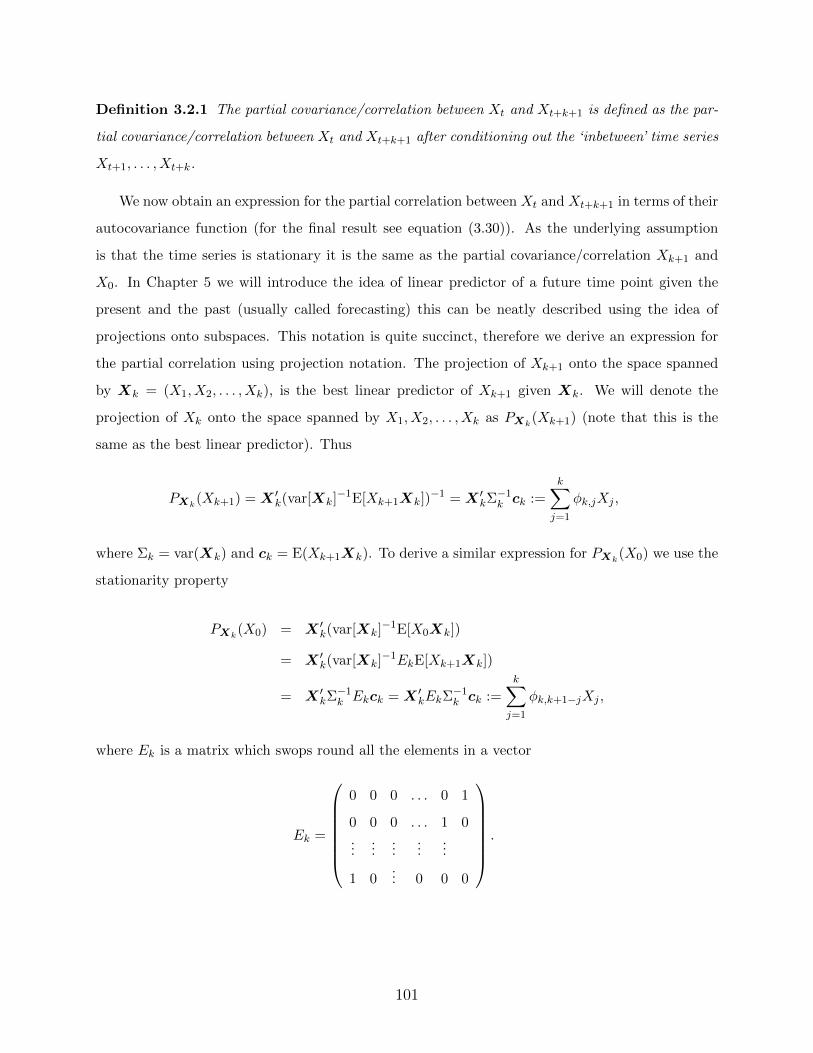
Definition 3.2.1 The partial covariance/correlation between Xt and Xt+k+1

is defined as the par-

tial covariance/correlation between Xt and Xt+k+1

after conditioning out the ‘inbetween’ time series

Xt+1

, . . . , Xt+k.

We now obtain an expression for the partial correlation between Xt and Xt+k+1

in terms of their

autocovariance function (for the final result see equation (3.30)). As the underlying assumption

is that the time series is stationary it is the same as the partial covariance/correlation Xk+1

and

X0

. In Chapter 5 we will introduce the idea of linear predictor of a future time point given the

present and the past (usually called forecasting) this can be neatly described using the idea of

projections onto subspaces. This notation is quite succinct, therefore we derive an expression for

the partial correlation using projection notation. The projection of Xk+1

onto the space spanned

by Xk = (X1

, X2

, . . . , Xk), is the best linear predictor of Xk+1

given Xk. We will denote the

projection of Xk onto the space spanned by X1

, X2

, . . . , Xk as PXk

(Xk+1

) (note that this is the

same as the best linear predictor). Thus

PXk

(Xk+1

) = X 0k(var[Xk]

�1E[Xk+1

Xk])�1 = X 0

k⌃�1

k ck :=k

X

j=1

�k,jXj ,

where ⌃k = var(Xk) and ck = E(Xk+1

Xk). To derive a similar expression for PXk

(X0

) we use the

stationarity property

PXk

(X0

) = X 0k(var[Xk]

�1E[X0

Xk])

= X 0k(var[Xk]

�1EkE[Xk+1

Xk])

= X 0k⌃

�1

k Ekck = X 0kEk⌃

�1

k ck :=k

X

j=1

�k,k+1�jXj ,

where Ek is a matrix which swops round all the elements in a vector

Ek =

0

B

B

B

B

B

B

@

0 0 0 . . . 0 1

0 0 0 . . . 1 0...

......

......

1 0... 0 0 0

1

C

C

C

C

C

C

A

.

101

Thus the partial correlation between Xt and Xt+k (where k > 0) is the correlation X0

� PXk

(X0

)

and Xk+1

� PXk

(Xk+1

), some algebra gives

cov(Xk+1

� PXk

(Xk+1

), X0

� PXk

(X0

)) = cov(Xk+1

X0

)� c0k⌃�1

k Ekck (3.30)

) cor(Xk+1

� PXk

(Xk+1

), X0

� PXk

(X0

)) =cov(Xk+1

X0

)� c0k⌃�1

k Ekckvar[Xk � PX

k

(X0

)].

We use this expression later to show that the partial correlations is also the last coe�cient for the

best linear predictor of Xk+1

given Xk. Note this can almost be seen from equation (3.25) i.e.

�t+1,1 = ⇢t+1,1

q

⌃

t+1,t+1

⌃

1,1

, however the next step is to show that ⌃t+1,t+1 = ⌃1,1 (however this can

be reasoned by using (3.17)).

We consider an example.

Example 3.2.1 (The PACF of an AR(1) process) Consider the causal AR(1) process Xt =

0.5Xt�1

+ "t where E("t) = 0 and var("t) = 1. Using (3.1) it can be shown that cov(Xt, Xt�2

) =

2⇥0.52 (compare with the MA(1) process Xt = "t+0.5"t�1

, where the covariance cov(Xt, Xt�2

) = 0).

We evaluate the partial covariance between Xt and Xt�2

. Remember we have to ‘condition out’ the

random variables inbetween, which in this case is Xt�1

. It is clear that the projection of Xt onto

Xt�1

is 0.5Xt�1

(since Xt = 0.5Xt�1

+ "t). Therefore Xt � Psp(Xt�1

)

Xt = Xt � 0.5Xt�1

= "t. The

projection of Xt�2

onto Xt�1

is a little more complicated, it is Psp(Xt�1

)

Xt�2

= E(Xt�1

Xt�2

)

E(X2

t�1

)

Xt�1

.

Therefore the partial correlation between Xt and Xt�2

cov�

Xt � PXt�1

Xt, Xt�2

� PXt�1

)

Xt�2

�

= cov

✓

"t, Xt�2

� E(Xt�1

Xt�2

)

E(X2

t�1

)Xt�1

◆

= 0.

In fact the above is true for the partial covariance between Xt and Xt�k, for all k � 2. Hence we

see that despite the covariance not being zero for the autocovariance of an AR process greater than

order two, the partial covariance is zero for all lags greater than or equal to two.

Using the same argument as above, it is easy to show that partial covariance of an AR(p) for

lags greater than p is zero. Hence in may respects the partial covariance can be considered as an

analogue of the autocovariance. It should be noted that though the covariance of MA(q) is zero

for lag greater than q, the same is not true for the parial covariance. Whereas partial covariances

removes correlation for autoregressive processes it seems to ‘add’ correlation for moving average

processes!

Model identification:

102

• If the autocovariances after a certain lag are zero q, it may be appropriate to fit an MA(q)

model to the time series.

On the other hand, the autocovariances of any AR(p) process will only decay to zero as the

lag increases.

• If the partial autocovariances after a certain lag are zero p, it may be appropriate to fit an

AR(p) model to the time series.

On the other hand, the partial covariances of any MA(p) process will only decay to zero as

the lag increases.

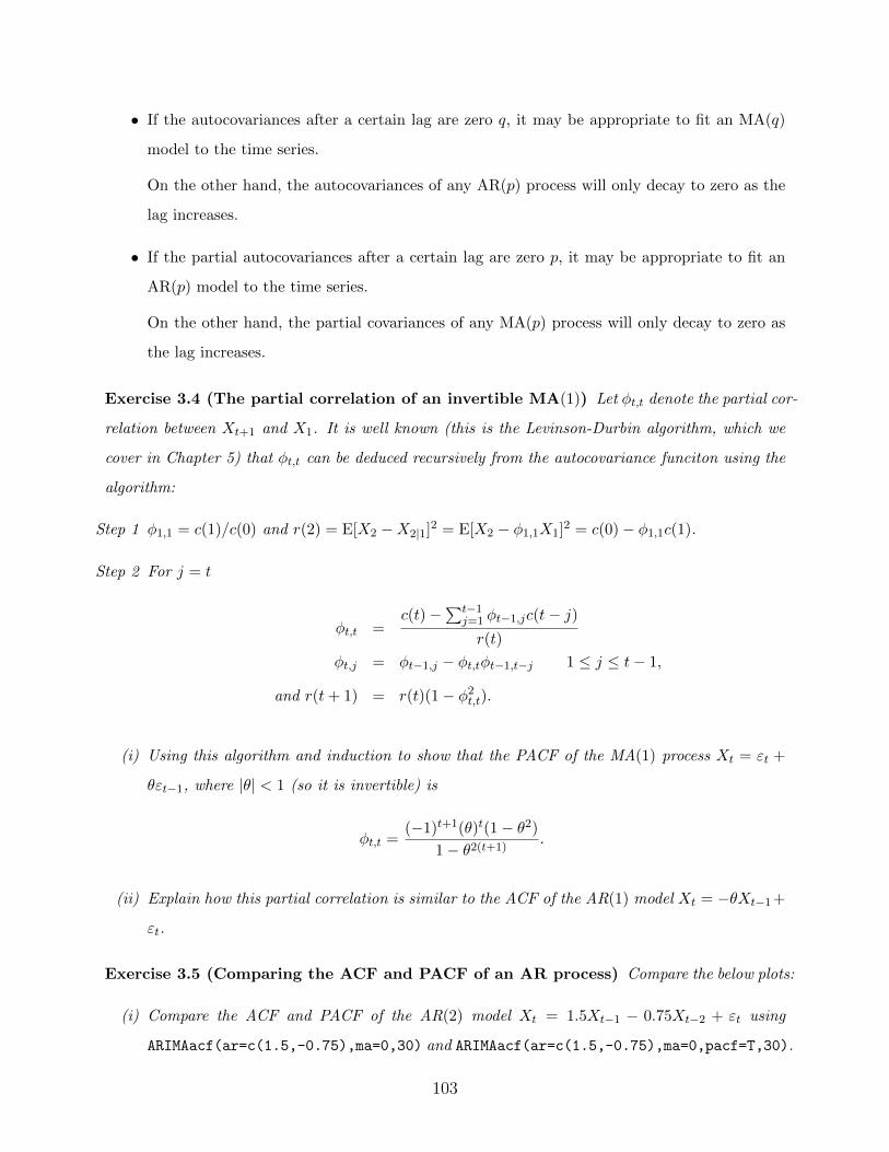
Exercise 3.4 (The partial correlation of an invertible MA(1)) Let �t,t denote the partial cor-

relation between Xt+1

and X1

. It is well known (this is the Levinson-Durbin algorithm, which we

cover in Chapter 5) that �t,t can be deduced recursively from the autocovariance funciton using the

algorithm:

Step 1 �1,1 = c(1)/c(0) and r(2) = E[X

2

�X2|1]

2 = E[X2

� �1,1X1

]2 = c(0)� �1,1c(1).

Step 2 For j = t

�t,t =c(t)�Pt�1

j=1

�t�1,jc(t� j)

r(t)

�t,j = �t�1,j � �t,t�t�1,t�j 1 j t� 1,

and r(t+ 1) = r(t)(1� �2t,t).

(i) Using this algorithm and induction to show that the PACF of the MA(1) process Xt = "t +

✓"t�1

, where |✓| < 1 (so it is invertible) is

�t,t =(�1)t+1(✓)t(1� ✓2)

1� ✓2(t+1)

.

(ii) Explain how this partial correlation is similar to the ACF of the AR(1) model Xt = �✓Xt�1

+

"t.

Exercise 3.5 (Comparing the ACF and PACF of an AR process) Compare the below plots:

(i) Compare the ACF and PACF of the AR(2) model Xt = 1.5Xt�1

� 0.75Xt�2

+ "t using

ARIMAacf(ar=c(1.5,-0.75),ma=0,30) and ARIMAacf(ar=c(1.5,-0.75),ma=0,pacf=T,30).

103

(ii) Compare the ACF and PACF of the MA(1) model Xt = "t�0.5"t using ARIMAacf(ar=0,ma=c(-1.5),30)

and ARIMAacf(ar=0,ma=c(-1.5),pacf=T,30).

(ii) Compare the ACF and PACF of the ARMA(2, 1) model Xt�1.5Xt�1

+0.75Xt�2

= "t�0.5"t

using ARIMAacf(ar=c(1.5,-0.75),ma=c(-1.5),30) and

ARIMAacf(ar=c(1.5,0.75),ma=c(-1.5),pacf=T,30).

Exercise 3.6 Compare the ACF and PACF plots of the monthly temperature data from 1996-2014.

Would you fit an AR, MA or ARMA model to this data?

Rcode

The sample partial autocorrelation of a time series can be obtained using the command pacf.

However, remember just because the sample PACF is not zero, does not mean the true PACF is

non-zero. This is why we require the error bars. In Section 6.3.1 we show how these error bars are

derived. The surprisingly result is that the error bars of a PACF can be used “quite” reliably to

determine the order of an AR(p) process. We will use Remark 3.2.2 to show that if the order of the

autoregressive process is p the for lag r > p, the partial correlation is such that b�rr = N(0, n�1/2)

(thus giving rise to the [�1.96n�1/2, 1.96n�1/2] error bars). However, it should be noted that there

will still be correlation between the sample partial correlations. The surprising result, is that the

error bars for an ACF plot cannot be reliably used to determine the order of an MA(q) model.

3.2.3 The variance/covariance matrix and precision matrix of an

autoregressive and moving average process

Let us suppose that {Xt} is a stationary time series. In this section we consider the variance/co-

variance matrix var(Xk) = ⌃k, where Xk = (X1

, . . . , Xk)0. We will consider two cases (i) when

Xt follows an MA(p) models and (ii) when Xt follows an AR(p) model. The variance and inverse

of the variance matrices for both cases yield quite interesting results. We will use classical results

from multivariate analysis, stated in Section 3.2.1.

We recall that the variance/covariance matrix of a stationary time series has a (symmetric)

104

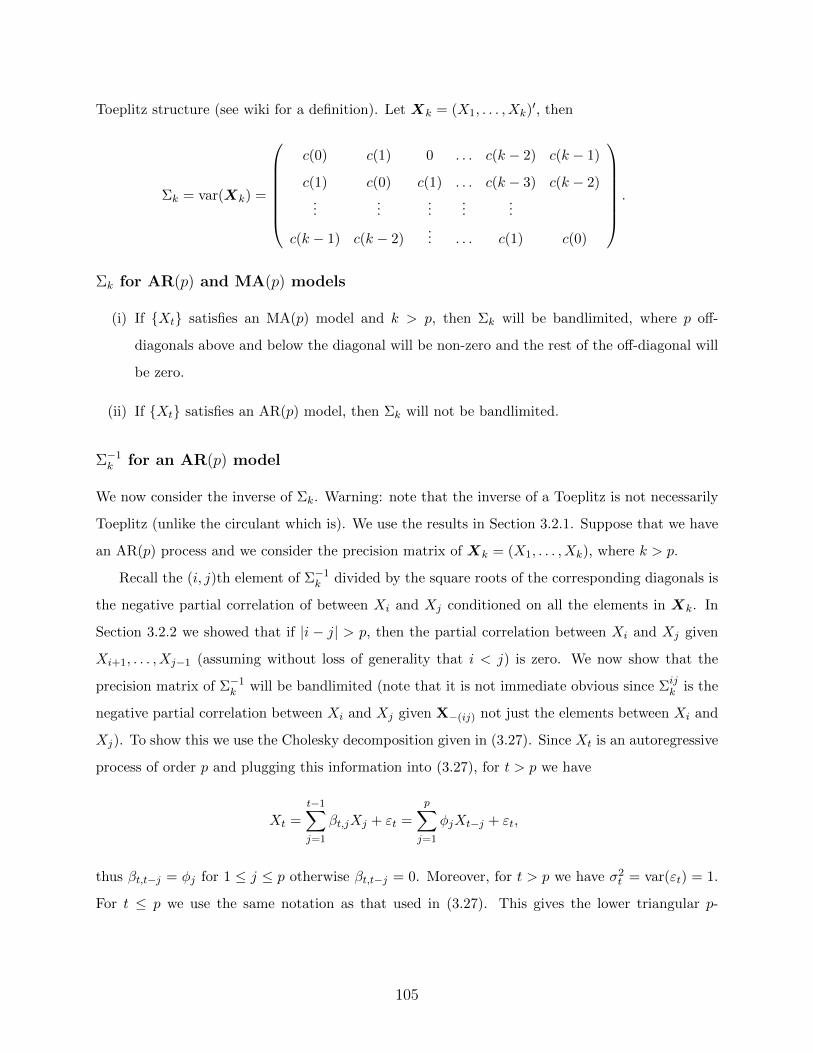
Toeplitz structure (see wiki for a definition). Let Xk = (X1

, . . . , Xk)0, then

⌃k = var(Xk) =

0

B

B

B

B

B

B

@

c(0) c(1) 0 . . . c(k � 2) c(k � 1)

c(1) c(0) c(1) . . . c(k � 3) c(k � 2)...

......

......

c(k � 1) c(k � 2)... . . . c(1) c(0)

1

C

C

C

C

C

C

A

.

⌃k for AR(p) and MA(p) models

(i) If {Xt} satisfies an MA(p) model and k > p, then ⌃k will be bandlimited, where p o↵-

diagonals above and below the diagonal will be non-zero and the rest of the o↵-diagonal will

be zero.

(ii) If {Xt} satisfies an AR(p) model, then ⌃k will not be bandlimited.

⌃�1

k for an AR(p) model

We now consider the inverse of ⌃k. Warning: note that the inverse of a Toeplitz is not necessarily

Toeplitz (unlike the circulant which is). We use the results in Section 3.2.1. Suppose that we have

an AR(p) process and we consider the precision matrix of Xk = (X1

, . . . , Xk), where k > p.

Recall the (i, j)th element of ⌃�1

k divided by the square roots of the corresponding diagonals is

the negative partial correlation of between Xi and Xj conditioned on all the elements in Xk. In

Section 3.2.2 we showed that if |i � j| > p, then the partial correlation between Xi and Xj given

Xi+1

, . . . , Xj�1

(assuming without loss of generality that i < j) is zero. We now show that the

precision matrix of ⌃�1

k will be bandlimited (note that it is not immediate obvious since ⌃ijk is the

negative partial correlation between Xi and Xj given X�(ij) not just the elements between Xi and

Xj). To show this we use the Cholesky decomposition given in (3.27). Since Xt is an autoregressive

process of order p and plugging this information into (3.27), for t > p we have

Xt =t�1

X

j=1

�t,jXj + "t =p

X

j=1

�jXt�j + "t,

thus �t,t�j = �j for 1 j p otherwise �t,t�j = 0. Moreover, for t > p we have �2t = var("t) = 1.

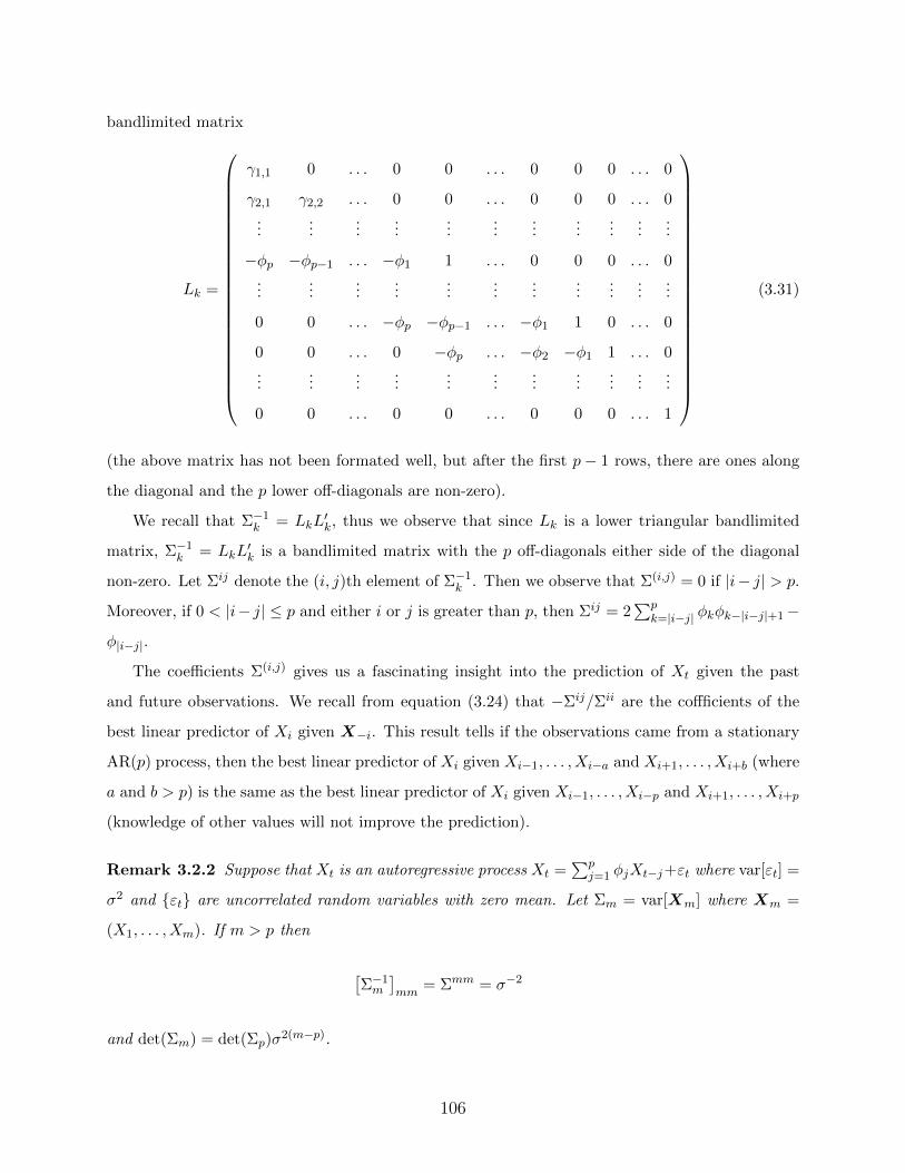
For t p we use the same notation as that used in (3.27). This gives the lower triangular p-

105

bandlimited matrix

Lk =

0

B

B

B

B

B

B

B

B

B

B

B

B

B

B

B

B

B

B

B

B

B

B

@

�1,1 0 . . . 0 0 . . . 0 0 0 . . . 0

�2,1 �

2,2 . . . 0 0 . . . 0 0 0 . . . 0...

......

......

......

......

......

��p ��p�1

. . . ��1

1 . . . 0 0 0 . . . 0...

......

......

......

......

......

0 0 . . . ��p ��p�1

. . . ��1

1 0 . . . 0

0 0 . . . 0 ��p . . . ��2

��1

1 . . . 0...

......

......

......

......

......

0 0 . . . 0 0 . . . 0 0 0 . . . 1

1

C

C

C

C

C

C

C

C

C

C

C

C

C

C

C

C

C

C

C

C

C

C

A

(3.31)

(the above matrix has not been formated well, but after the first p� 1 rows, there are ones along

the diagonal and the p lower o↵-diagonals are non-zero).

We recall that ⌃�1

k = LkL0k, thus we observe that since Lk is a lower triangular bandlimited

matrix, ⌃�1

k = LkL0k is a bandlimited matrix with the p o↵-diagonals either side of the diagonal

non-zero. Let ⌃ij denote the (i, j)th element of ⌃�1

k . Then we observe that ⌃(i,j) = 0 if |i� j| > p.

Moreover, if 0 < |i� j| p and either i or j is greater than p, then ⌃ij = 2Pp

k=|i�j| �k�k�|i�j|+1

��|i�j|.

The coe�cients ⌃(i,j) gives us a fascinating insight into the prediction of Xt given the past

and future observations. We recall from equation (3.24) that �⌃ij/⌃ii are the co↵ficients of the

best linear predictor of Xi given X�i. This result tells if the observations came from a stationary

AR(p) process, then the best linear predictor of Xi given Xi�1

, . . . , Xi�a and Xi+1

, . . . , Xi+b (where

a and b > p) is the same as the best linear predictor of Xi given Xi�1

, . . . , Xi�p and Xi+1

, . . . , Xi+p

(knowledge of other values will not improve the prediction).

Remark 3.2.2 Suppose that Xt is an autoregressive process Xt =Pp

j=1

�jXt�j+"t where var["t] =

�2 and {"t} are uncorrelated random variables with zero mean. Let ⌃m = var[Xm] where Xm =

(X1

, . . . , Xm). If m > p then

⇥

⌃�1

m

⇤

mm= ⌃mm = ��2

and det(⌃m) = det(⌃p)�2(m�p).

106

Exercise 3.7 Prove Remark 3.2.2.

3.3 Correlation and non-causal time series

Here we demonstrate that it is not possible to identify whether a process is noninvertible/noncausal

from its covariance structure. The simplest way to show result this uses the spectral density

function, which will now define and then return to and study in depth in Chapter 8.

Definition 3.3.1 (The spectral density) Given the covariances c(k) (withP

k |c(k)|2 < 1) the

spectral density function is defined as

f(!) =X

k

c(k) exp(ik!).

The covariances can be obtained from the spectral density by using the inverse fourier transform

c(k) =1

2⇡

Z

2⇡

0

f(!) exp(�ik!).

Hence the covariance yields the spectral density and visa-versa.

For reference below, we point out that the spectral density function uniquely identifies the autoco-

variance function.

Let us suppose that {Xt} satisfies the AR(p) representation

Xt =p

X

i=1

�iXt�i + "t

where var("t) = 1 and the roots of �(z) = 1�Ppj=1

�jzj can lie inside and outside the unit circle,

but not on the unit circle (thus it has a stationary solution). We will show in Chapter 8 that the

spectral density of this AR process is

f(!) =1

|1�Ppj=1

�j exp(ij!)|2 . (3.32)

• Factorizing f(!).

Let us supose the roots of the characteristic polynomial �(z) = 1 +Pq

j=1

�jzj are {�j}pj=1

,

thus we can factorize �(x) 1 +Pp

j=1

�jzj =Qp

j=1

(1� �jz). Using this factorization we have

107

(3.32) can be written as

f(!) =1

Qpj=1

|1� �j exp(i!)|2. (3.33)

As we have not assumed {Xt} is causal, the roots of �(z) can lie both inside and outside the

unit circle. We separate the roots, into those outside the unit circle {�O,j1

; j1

= 1, . . . , p1

}and inside the unit circle {�I,j

2

; j2

= 1, . . . , p2

} (p1

+ p2

= p). Thus

�(z) = [p1

Y

j1

=1

(1� �O,j1

z)][p2

Y

j2

=1

(1� �I,j2

z)]

= (�1)p2�I,j2

z�p2 [

p1

Y

j1

=1

(1� �O,j1

z)][p2

Y

j2

=1

(1� ��1

I,j2

z)]. (3.34)

Thus we can rewrite the spectral density in (3.35)

f(!) =1

Qp2

j2

=1

|�I,j2

|21

Qp1

j1

=1

|1� �O,j exp(i!)|2Qp

2

j2

=1

|1� ��1

I,j2

exp(i!)|2 . (3.35)

Let

fO(!) =1

Qp1

j1

=1

|1� �O,j exp(i!)|2Qp

2

j2

=1

|1� ��1

I,j2

exp(i!)|2 .

Then f(!) =Qp

2

j2

=1

|�I,j2

|�2fO(!).

• A parallel causal AR(p) process with the same covariance structure always exists.

We now define a process which has the same autocovariance function as {Xt} but is causal.

Using (3.34) we define the polynomial

e�(z) = [p1

Y

j1

=1

(1� �O,j1

z)][p2

Y

j2

=1

(1� ��1

I,j2

z)]. (3.36)

By construction, the roots of this polynomial lie outside the unit circle. We then define the

AR(p) process

e�(B) eXt = "t, (3.37)

from Lemma 2.3.1 we know that { eXt} has a stationary, almost sure unique solution. More-

108

over, because the roots lie outside the unit circle the solution is causal.

By using (3.32) the spectral density of { eXt} is ef(!). We know that the spectral density

function uniquely gives the autocovariance function. Comparing the spectral density of { eXt}with the spectral density of {Xt} we see that they both are the same up to a multiplicative

constant. Thus they both have the same autocovariance structure up to a multiplicative

constant (which can be made the same, if in the definition (3.37) the innovation process has

varianceQp

2

j2

=1

|�I,j2

|�2).

Therefore, for every non-causal process, there exists a causal process with the same autoco-

variance function.

By using the same arguments above, we can generalize to result to ARMA processes.

Definition 3.3.2 An ARMA process is said to have minimum phase when the roots of �(z) and

✓(z) both lie outside of the unit circle.

Remark 3.3.1 For Gaussian random processes it is impossible to discriminate between a causal

and non-causal time series, this is because the mean and autocovariance function uniquely identify

the process.

However, if the innovations are non-Gaussian, even though the autocovariance function is ‘blind’

to non-causal processes, by looking for other features in the time series we are able to discriminate

between a causal and non-causal process.

3.3.1 The Yule-Walker equations of a non-causal process

Once again let us consider the zero mean AR(p) model

Xt =p

X

j=1

�jXt�j + "t,

and var("t) < 1. Suppose the roots of the corresponding characteristic polynomial lie outside the

unit circle, then {Xt} is strictly stationary where the solution of Xt is only in terms of past and

present values of {"t}. Moreover, it is second order stationary with covariance {c(k)}. We recall

from Section 3.1.2, equation (3.4) that we derived the Yule-Walker equations for causal AR(p)

109

processes, where

E(XtXt�k) =p

X

j=1

�jE(Xt�jXt�k) ) c(k)�p

X

j=1

�jc(k � j) = 0. (3.38)

Let us now consider the case that the roots of the characteristic polynomial lie both outside

and inside the unit circle, thus Xt does not have a causal solution but it is still strictly and second

order stationary (with autocovariance, say {c(k)}). In the previous section we showed that there

exists a causal AR(p) e�(B) eXt = "t (where �(B) and e�(B) = 1 �Ppj=1

�jzj are the characteristic

polynomials defined in (3.34) and (3.36)). We showed that both have the same autocovariance

structure. Therefore,

c(k)�p

X

j=1

�jc(k � j) = 0

This means the Yule-Walker equations for {Xt} would actually give the AR(p) coe�cients of {Xt}.Thus if the Yule-Walker equations were used to estimate the AR coe�cients of {Xt}, in reality we

would be estimating the AR coe�cients of the corresponding causal {Xt}.

3.3.2 Filtering non-causal AR models

Here we discuss the surprising result that filtering a non-causal time series with the corresponding

causal AR parameters leaves a sequence which is uncorrelated but not independent. Let us suppose

that

Xt =p

X

j=1

�jXt�j + "t,

where "t are iid, E("t) = 0 and var("t) < 1. It is clear that given the input Xt, if we apply the

filter Xt �Pp

j=1

�jXt�j we obtain an iid sequence (which is {"t}).Suppose that we filter {Xt} with the causal coe�cients {e�j}, the output e"t = Xt�

Ppj=1

e�jXt�j

is not an independent sequence. However, it is an uncorrelated sequence. We illustrate this with an

example.

Example 3.3.1 Let us return to the AR(1) example, where Xt = �Xt�1

+ "t. Let us suppose that

110

� > 1, which corresponds to a non-causal time series, then Xt has the solution

Xt = �1X

j=1

1

�j"t+j+1

.

The causal time series with the same covariance structure as Xt is eXt = 1

�eXt�1

+ " (which has

backshift representation (1� 1/(�B))Xt = "t). Suppose we pass Xt through the causal filter

e"t = (1� 1

�B)Xt = Xt � 1

�Xt�1

= �(1� 1

�B)

B(1� 1

�B )"t

= � 1

�"t + (1� 1

�2)

1X

j=1

1

�j�1

"t+j .

Evaluating the covariance of the above (assuming wlog that var(") = 1) is

cov(e"t, e"t+r) = � 1

�(1� 1

�2)1

�r+ (1� 1

�2)2

1X

j=0

1

�2j= 0.

Thus we see that {e"t} is an uncorrelated sequence, but unless it is Gaussian it is clearly not inde-

pendent. One method to study the higher order dependence of {e"t}, by considering it’s higher order

cumulant structure etc.

The above above result can be generalised to general AR models, and it is relatively straightforward

to prove using the Cramer representation of a stationary process (see Section 8.4, Theorem ??).

Exercise 3.8 (i) Consider the causal AR(p) process

Xt = 1.5Xt�1

� 0.75Xt�2

+ "t.

Derive a parallel process with the same autocovariance structure but that is non-causal (it

should be real).

(ii) Simulate both from the causal process above and the corresponding non-causal process with

non-Gaussian innovations (see Section 2.6). Show that they have the same ACF function.

(iii) Find features which allow you to discriminate between the causal and non-causal process.

111