STAT 497

LECTURE NOTES 2

1

THE AUTOCOVARIANCE AND THE AUTOCORRELATION FUNCTIONS

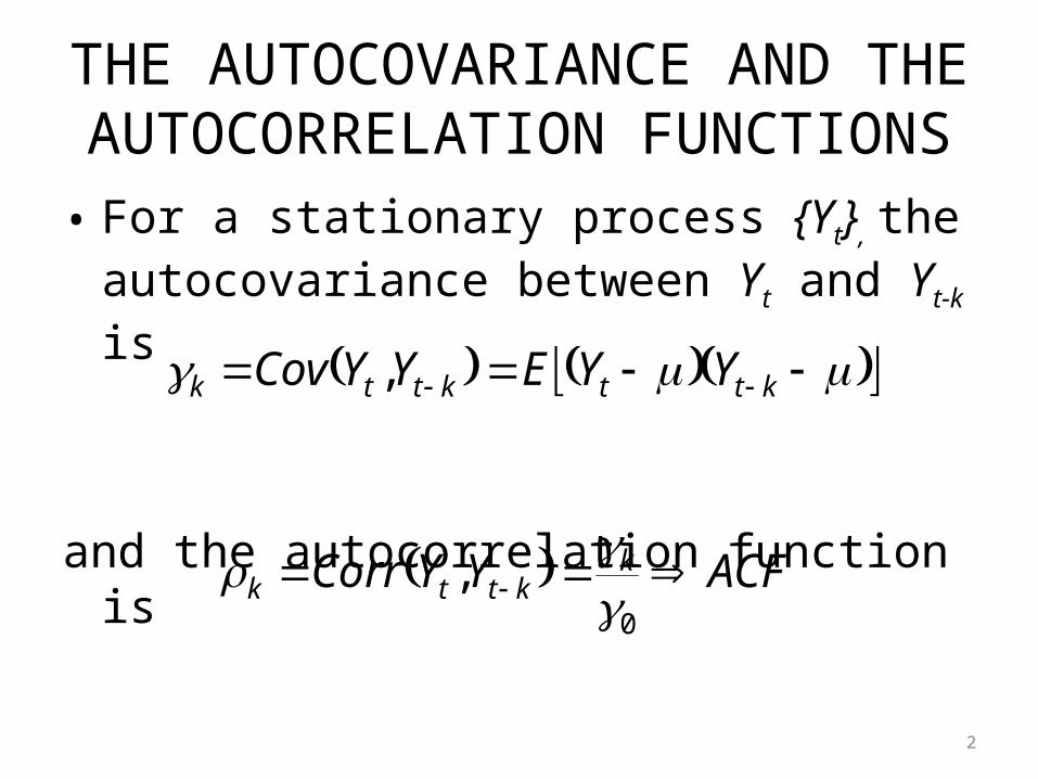
• For a stationary process {Yt}, the autocovariance between Yt and Yt-k is

and the autocorrelation function is

kttkttk YYEYYCov ,

ACFYYCorr kkttk

0

,

2

THE AUTOCOVARIANCE AND THE AUTOCORRELATION FUNCTIONS

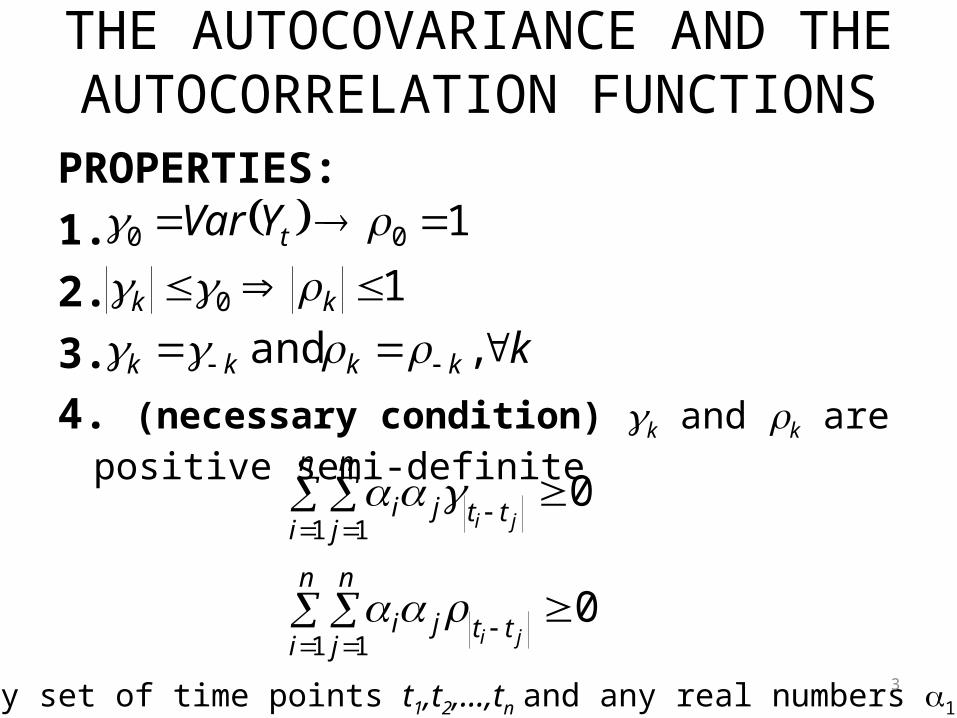
PROPERTIES:1. 2.3.4. (necessary condition) k and k are positive semi-

definite

.100 tYVar

.10 kk ., and kkkkk

0

0

1 1

1 1

n

i

n

jttji

n

i

n

jttji

ji

ji

for any set of time points t1,t2,…,tn and any real numbers 1,2,…,n.3

THE PARTIAL AUTOCORRELATION FUNCTION (PACF)

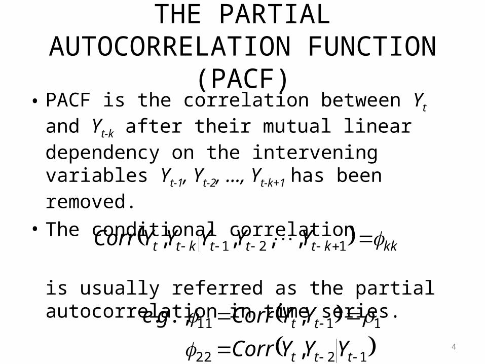
• PACF is the correlation between Yt and Yt-k after their mutual linear dependency on the intervening variables Yt-1, Yt-2, …, Yt-k+1 has been removed.

• The conditional correlation

is usually referred as the partial autocorrelation in time series.

kkktttktt YYYYYCorr 121 ,,,,

1222

1111

,

, .,.

ttt

tt

YYYCorr

YYCorrge

4

CALCULATION OF PACF

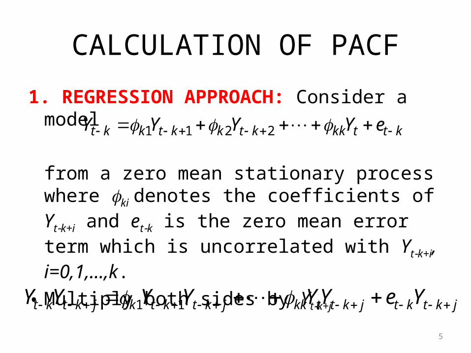
1. REGRESSION APPROACH: Consider a model

from a zero mean stationary process where ki denotes the coefficients of Ytk+i and etk is the zero mean error term which is uncorrelated with Ytk+i, i=0,1,…,k.

• Multiply both sides by Ytk+j

kttkkktkktkkt eYYYY 2211

jktktjkttkkjktktkjktkt YeYYYYYY 11

5

CALCULATION OF PACF

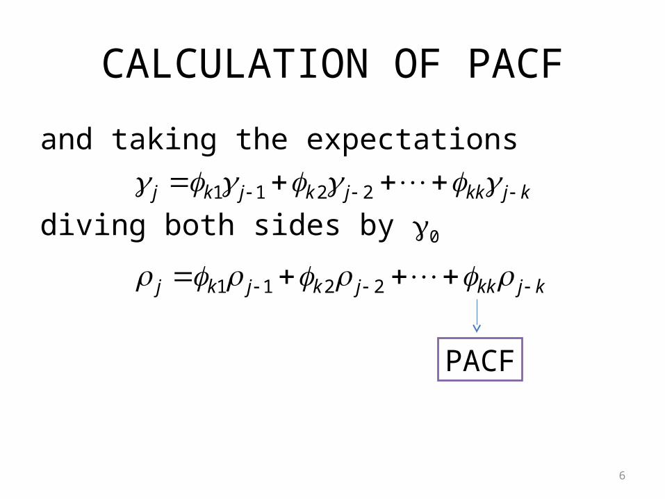
and taking the expectations

diving both sides by 0

kjkkjkjkj 2211

kjkkjkjkj 2211

PACF

6

CALCULATION OF PACF

• For j=1,2,…,k, we have the following system of equations

kkkkkkk

kkkkk

kkkkk

2211

22112

11211

7

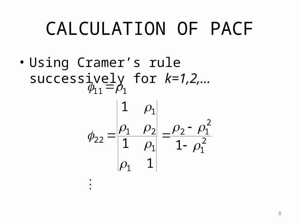
CALCULATION OF PACF

• Using Cramer’s rule successively for k=1,2,…

21

212

1

1

21

1

22

111

11

1

1

8

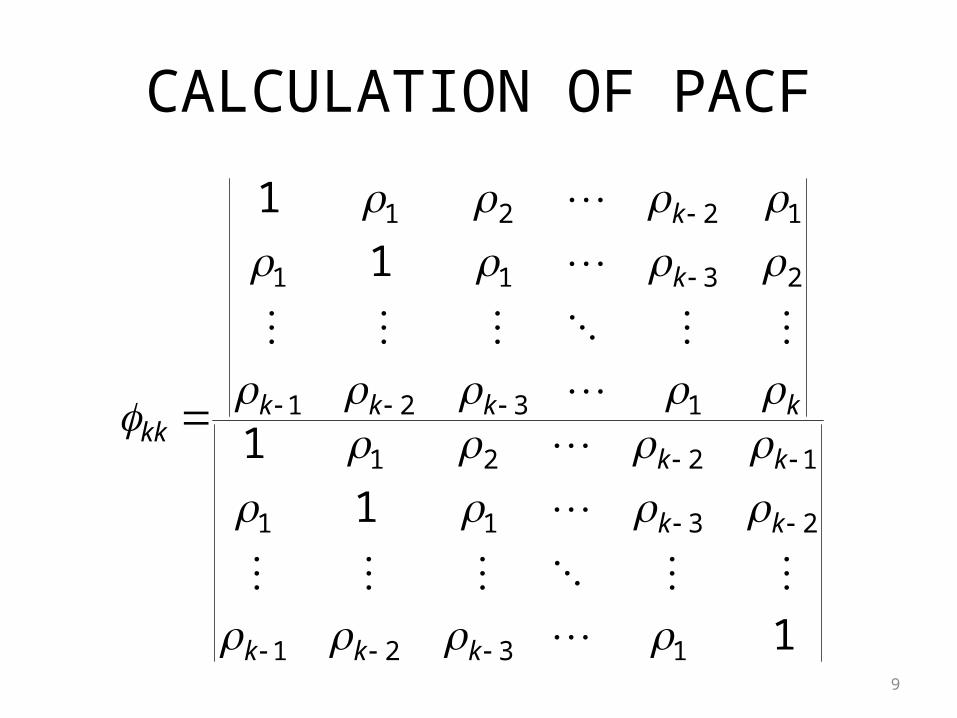
CALCULATION OF PACF

1

1

1

1

1

1321

2311

1221

1321

2311

1221

kkk

kk

kk

kkkk

k

k

kk

9

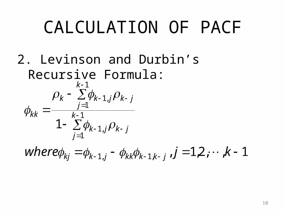
CALCULATION OF PACF

2. Levinson and Durbin’s Recursive Formula:

.1,,2,1,

1

,1,1

1

1,1

1

1,1

kjwhere jkkkkjkkj

k

jjkjk

k

jjkjkk

kk

10

WHITE NOISE (WN) PROCESS

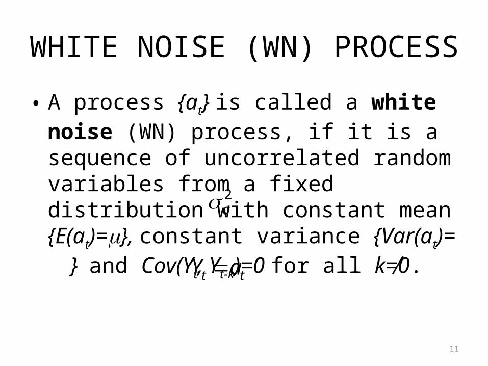
• A process {at} is called a white noise (WN) process, if it is a sequence of uncorrelated random variables from a fixed distribution with constant mean {E(at)=}, constant variance {Var(at)= } and Cov(Yt, Yt-k)=0 for all k≠0.

2a

tt aY

11

WHITE NOISE (WN) PROCESS

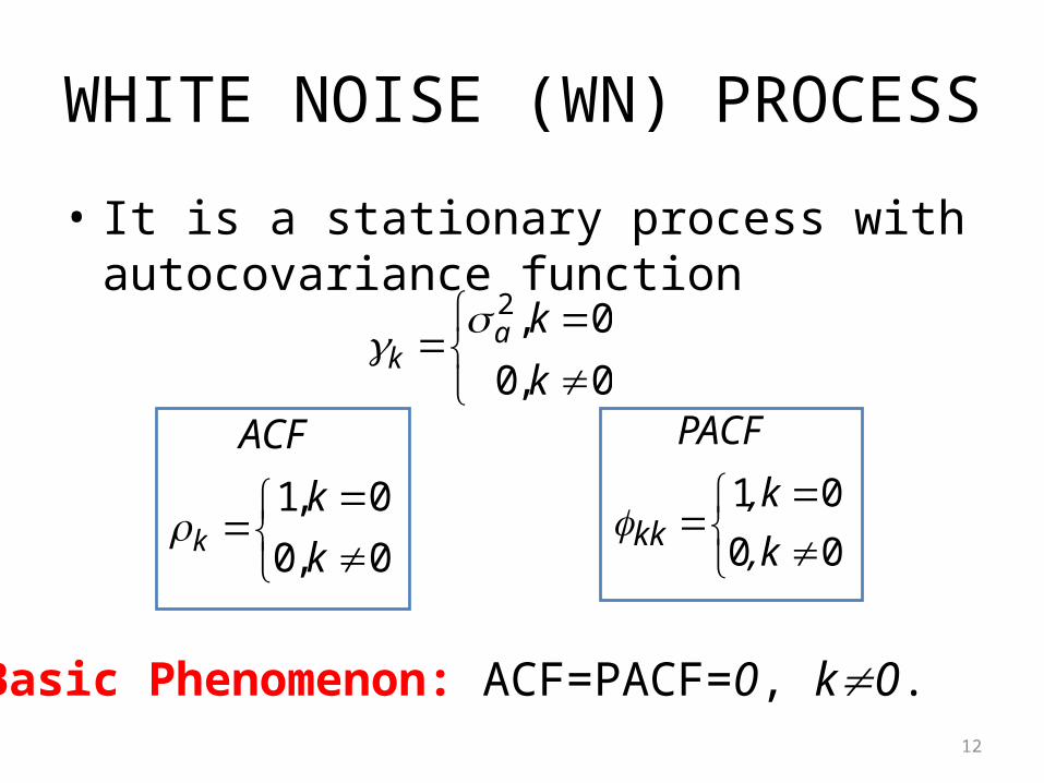
• It is a stationary process with autocovariance function

12

0,0

0,2

k

kak

0,0

0,1

k

k

ACF

k

00

01

k,

k,

PACF

kk

Basic Phenomenon: ACF=PACF=0, k0.

WHITE NOISE (WN) PROCESS

• White noise (in spectral analysis): white light is produced in which all frequencies (i.e., colors) are present in equal amount.

• Memoryless process• Building block from which we can construct

more complicated models• It plays the role of an orthogonal basis in the

general vector and function analysis.

13

ESTIMATION OF THE MEAN, AUTOCOVARIANCE AND AUTOCORRELATION

14

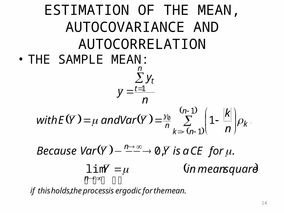
• THE SAMPLE MEAN:

n

yy

n

tt

1

.1

1

1

0k

n

nkn n

kYVar and YE with

. for CE a is YYVar Because n ,0

squaremean inY

mean. the for ergodic is process the holds, this if

n

lim

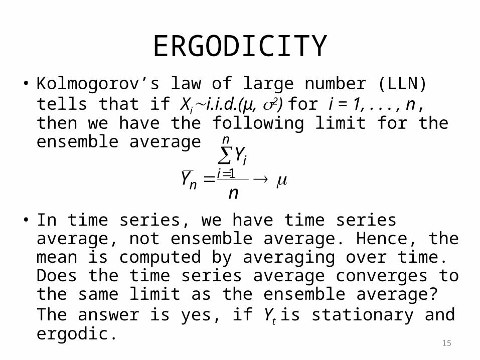
ERGODICITY• Kolmogorov’s law of large number (LLN) tells that if

Xii.i.d.(μ, 2) for i = 1, . . . , n, then we have the following limit for the ensemble average

• In time series, we have time series average, not ensemble average. Hence, the mean is computed by averaging over time. Does the time series average converges to the same limit as the ensemble average? The answer is yes, if Yt is stationary and ergodic.

15

.1

n

YY

n

ii

n

ERGODICITY• A covariance stationary process is said to

ergodic for the mean, if the time series average converges to the population mean.

• Similarly, if the sample average provides an consistent estimate for the second moment, then the process is said to be ergodic for the second moment.

16

ERGODICITY

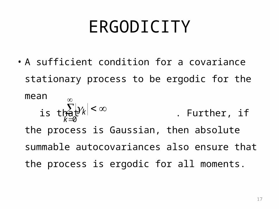
• A sufficient condition for a covariance

stationary process to be ergodic for the mean

is that . Further, if the process is

Gaussian, then absolute summable

autocovariances also ensure that the process

is ergodic for all moments.

17

0kk

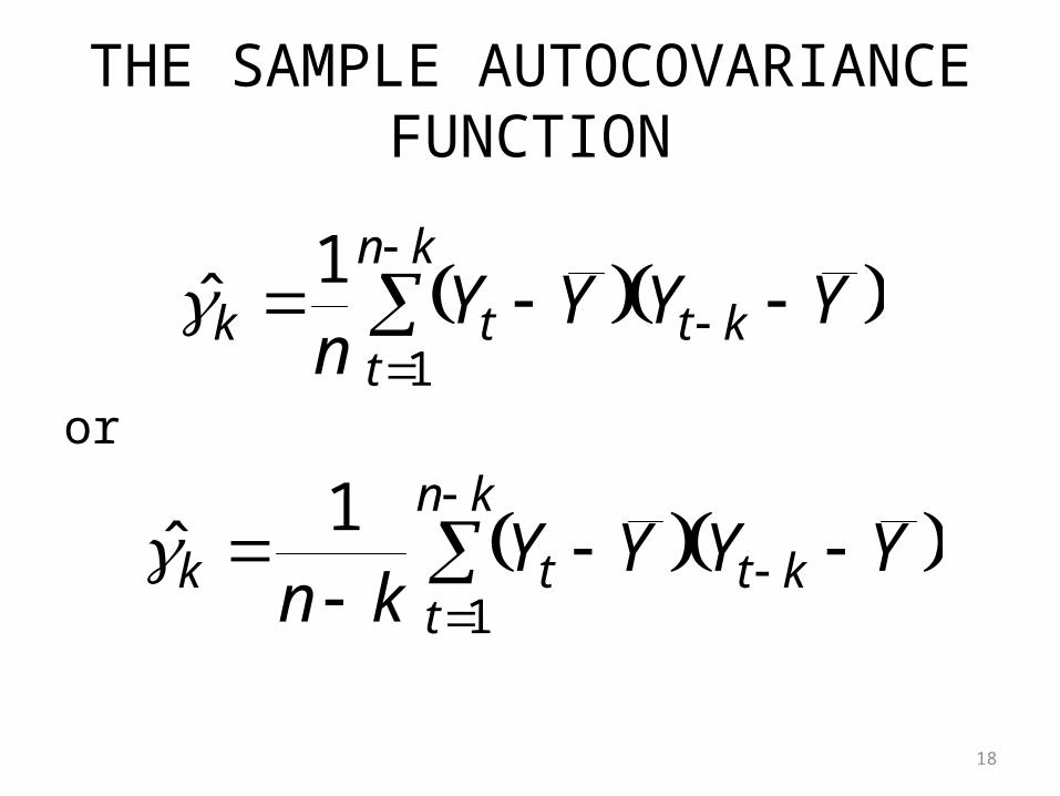
THE SAMPLE AUTOCOVARIANCE FUNCTION

or

18

YYYYn kt

kn

ttk

1

1

YYYYkn kt

kn

ttk

1

1

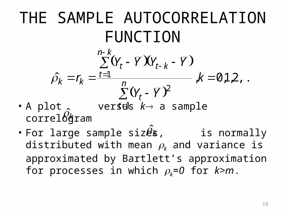
THE SAMPLE AUTOCORRELATION FUNCTION

• A plot versus k a sample correlogram• For large sample sizes, is normally

distributed with mean k and variance is approximated by Bartlett’s approximation for processes in which k=0 for k>m.

19

,...2,1,0,ˆ

1

2

1

kYY

YYYYr n

tt

kt

kn

tt

kk

k

k

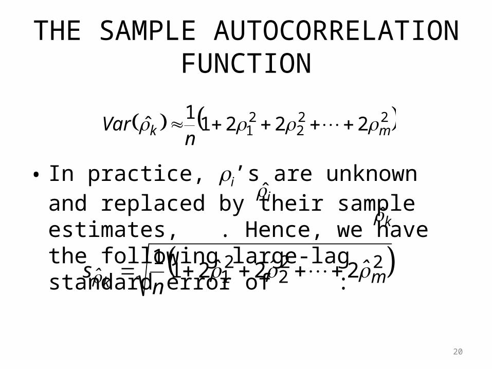
THE SAMPLE AUTOCORRELATION FUNCTION

• In practice, i’s are unknown and replaced by their sample estimates, . Hence, we have the following large-lag standard error of :

20

i

222

21 2221

1ˆ mk n

Var

k

222

21 2221

1mˆ ˆˆˆ

ns

k

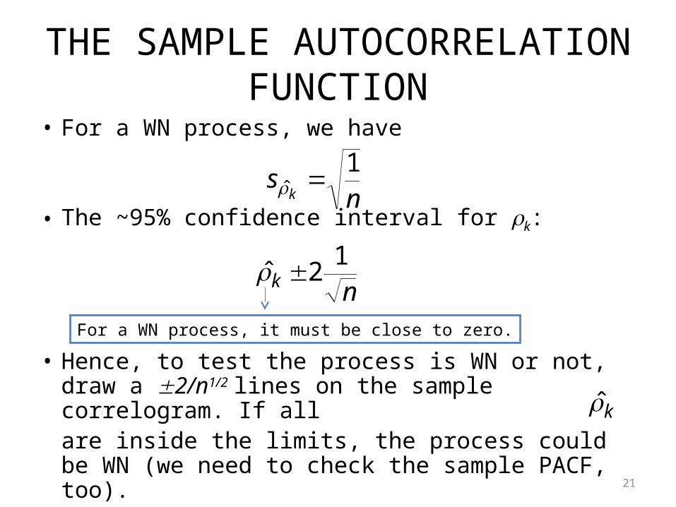
THE SAMPLE AUTOCORRELATION FUNCTION

• For a WN process, we have

• The ~95% confidence interval for k:

• Hence, to test the process is WN or not, draw a 2/n1/2 lines on the sample correlogram. If all

are inside the limits, the process could be WN (we need to check the sample PACF, too). 21

ns

k

1ˆ

nk1

2ˆ

For a WN process, it must be close to zero.

k

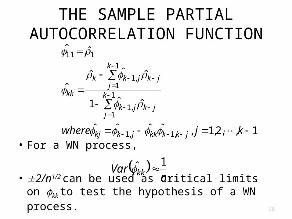
THE SAMPLE PARTIAL AUTOCORRELATION FUNCTION

• For a WN process,

• 2/n1/2 can be used as critical limits on kk to test the hypothesis of a WN process. 22

.1,,2,1,ˆˆˆˆ

ˆˆ1

ˆˆˆˆ

ˆˆ

,1,1

1

1,1

1

1,1

111

kj where jkkkkjkkj

k

jjkjk

k

jjkjkk

kk

n

Var kk1ˆ

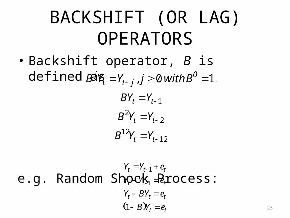
BACKSHIFT (OR LAG) OPERATORS

• Backshift operator, B is defined as

e.g. Random Shock Process:

23

.10, 0

jttj B withjYYB

1212

22

1

tt

tt

tt

YYB

YYB

YBY

tt

ttt

ttt

ttt

eYB

eBYY

eYY

eYY

1

1

1

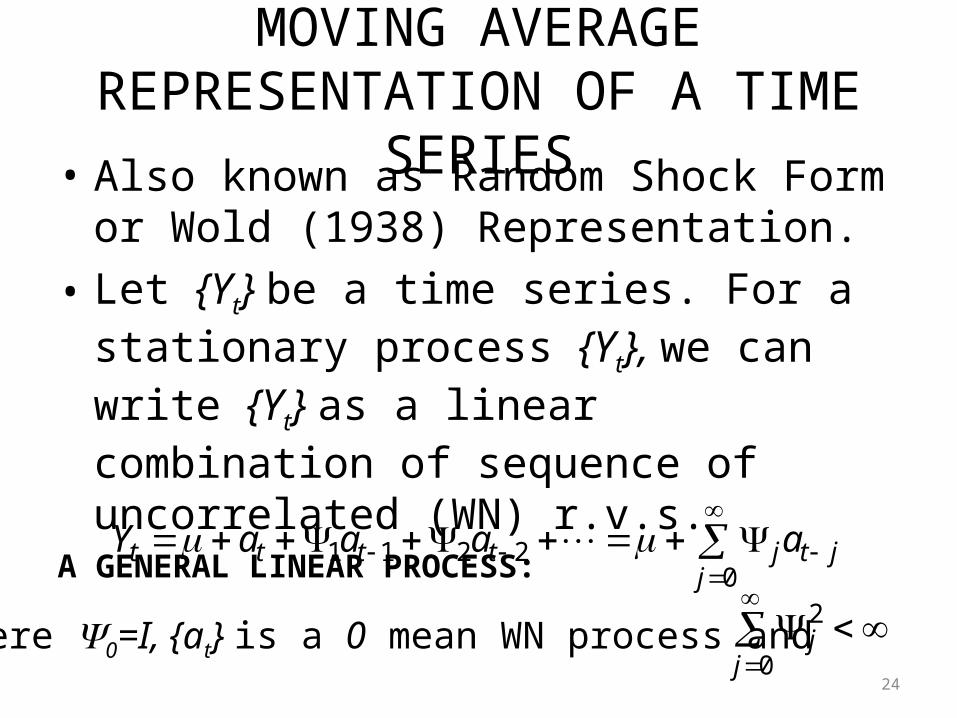
MOVING AVERAGE REPRESENTATION OF A TIME SERIES

• Also known as Random Shock Form or Wold (1938) Representation.

• Let {Yt} be a time series. For a stationary process {Yt}, we can write {Yt} as a linear combination of sequence of uncorrelated (WN) r.v.s.

A GENERAL LINEAR PROCESS:

24

02211

jjtjtttt aaaaY

where 0=I, {at} is a 0 mean WN process and .0

2

jj

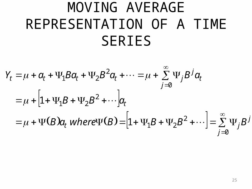
MOVING AVERAGE REPRESENTATION OF A TIME SERIES

25

0

221

221

0

221

1

1

j

jjt

t

jt

jjtttt

BBBB whereaB

aBB

aBaBBaaY

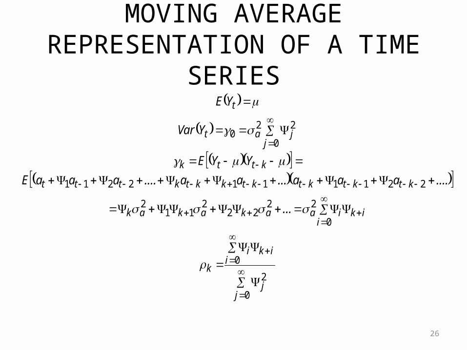
MOVING AVERAGE REPRESENTATION OF A TIME SERIES

26

0

2

0

0

2222

211

2

2211112211

0

220

jj

iiki

k

iikiaakakak

ktktktktkktkttt

kttk

jjat

t

...

....aaa...aa....aaaE

YYE

YVar

YE

MOVING AVERAGE REPRESENTATION OF A TIME SERIES

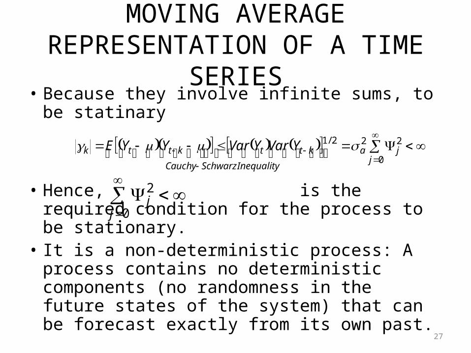
• Because they involve infinite sums, to be statinary

• Hence, is the required condition for the process to be stationary.

• It is a non-deterministic process: A process contains no deterministic components (no randomness in the future states of the system) that can be forecast exactly from its own past.

27

0

222/1

jja

Inequality SchwarzCauchy

kttkttk YVarYVarYYE

0

2

jj

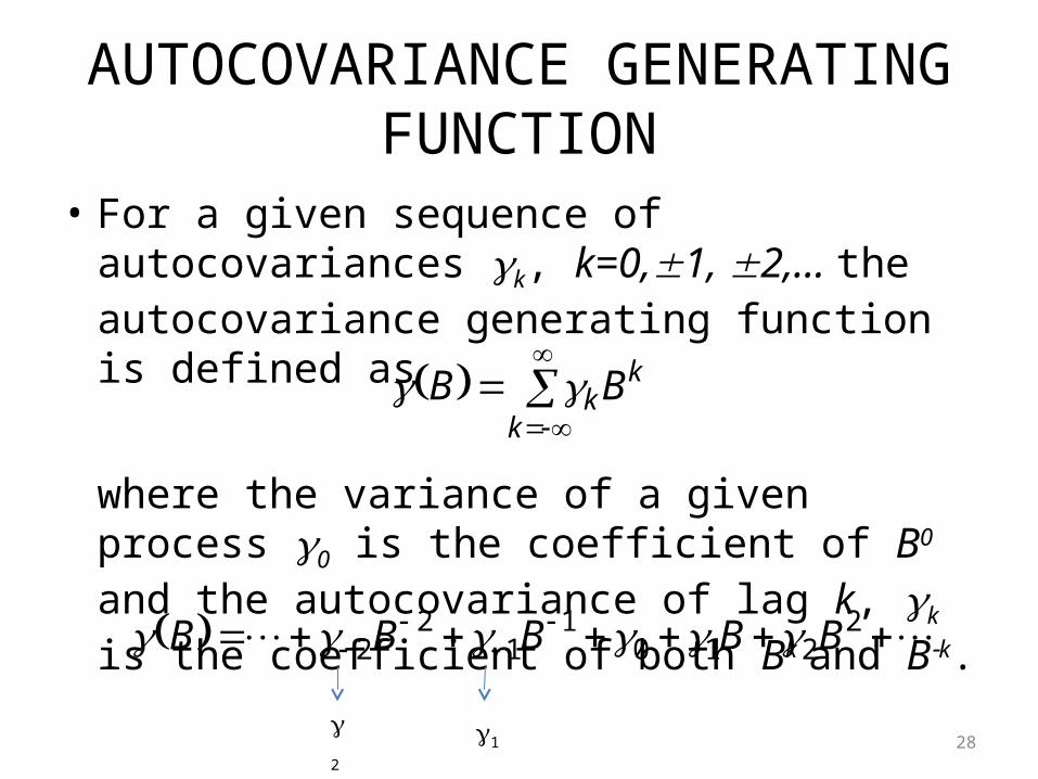
AUTOCOVARIANCE GENERATING FUNCTION

• For a given sequence of autocovariances k, k=0,1, 2,… the autocovariance generating function is defined as

where the variance of a given process 0 is the coefficient of B0 and the autocovariance of lag k, k is the coefficient of both Bk and Bk.

28

k

kk BB

2210

11

22 BBBBB

2 1

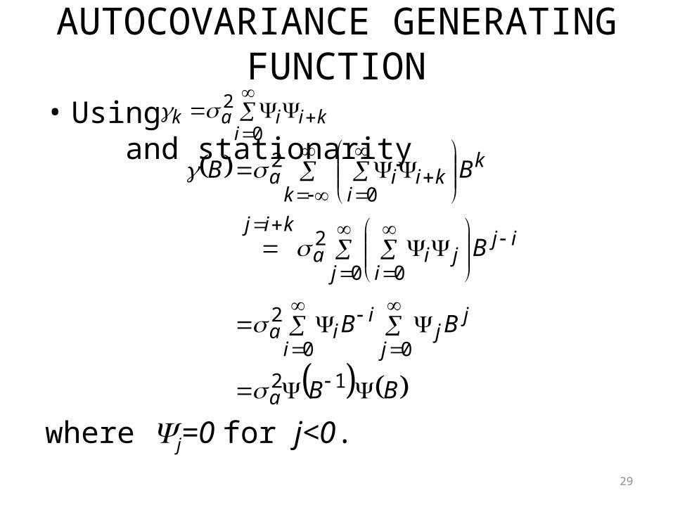
AUTOCOVARIANCE GENERATING FUNCTION

• Using and stationarity

29

0

2

ikiiak

B B

BB

B

BB

a

j

i jj

iia

ij

j ijia

kij

k

k ikiia

12

0 0

2

0 0

2

0

2

where j=0 for j<0.

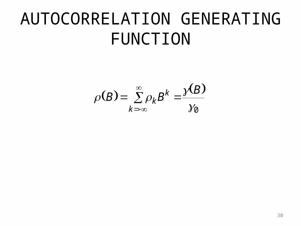
AUTOCORRELATION GENERATING FUNCTION

30

0

BBB

k

kk

EXAMPLE

a)Write the above equation in random shock form.

b)Find the autocovariance generating function.

31

.,0~1 21 atttt iida and whereaYY

AUTOREGRESSIVE REPRESENTATION OF A TIME SERIES

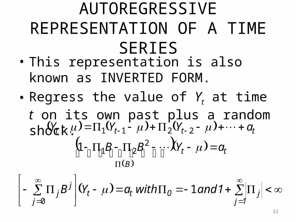
• This representation is also known as INVERTED FORM.

• Regress the value of Yt at time t on its own past plus a random shock.

32

.1

1

0

221

2211

1jj0tt

j

jj

tt

B

tttt

1 and withaYB

aYBB

aYYY

AUTOREGRESSIVE REPRESENTATION OF A TIME SERIES

• It is an invertible process (it is important for forecasting). Not every stationary process is invertible (Box and Jenkins, 1978).

• Invertibility provides uniqueness of the autocorrelation function.

• It means that different time series models can be re-expressed by each other.

33

INVERTIBILITY RULE USING THE RANDOM SHOCK FORM

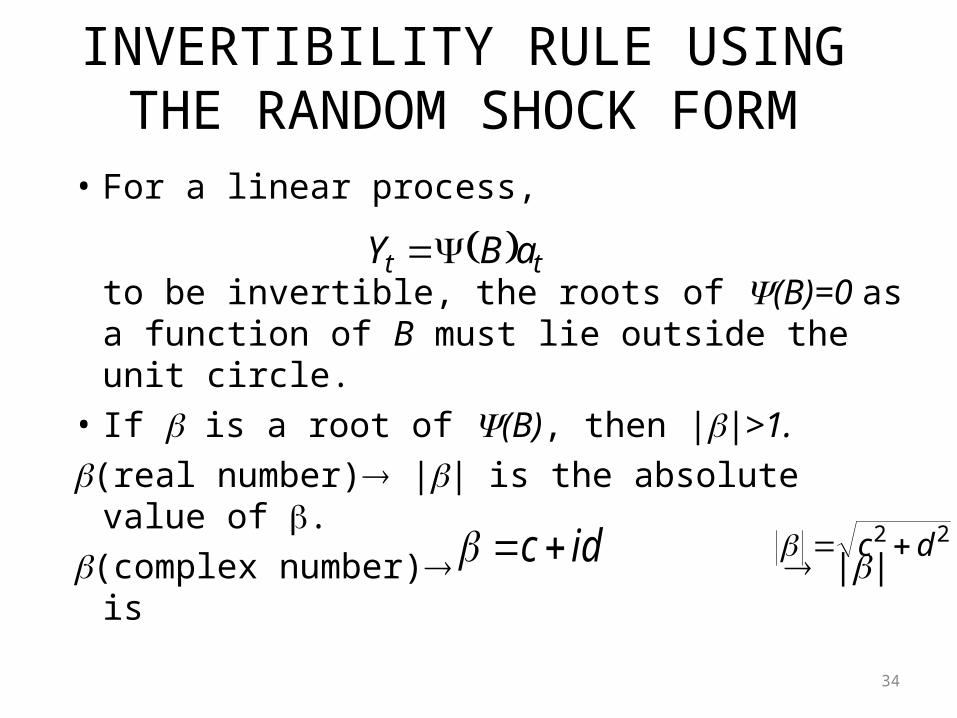
• For a linear process,

to be invertible, the roots of (B)=0 as a function of B must lie outside the unit circle.

• If is a root of (B), then ||>1.(real number) || is the absolute value of .(complex number) || is

34

tt aBY

idc .22 dc

INVERTIBILITY RULE USING THE RANDOM SHOCK FORM

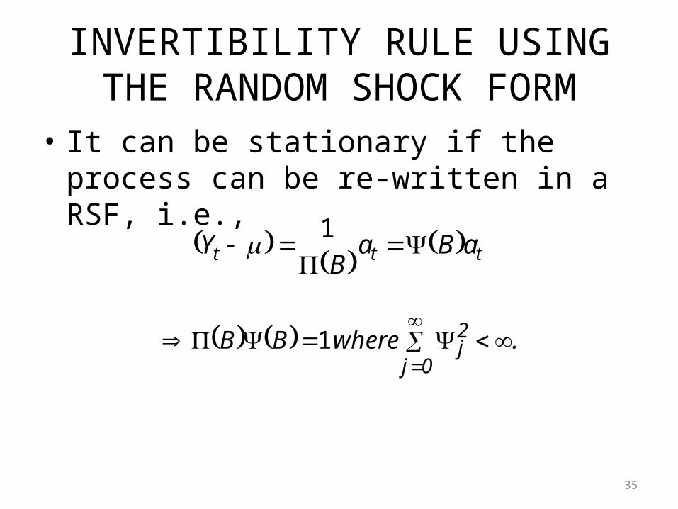
• It can be stationary if the process can be re-written in a RSF, i.e.,

35

ttt aBaB

Y

1

0j

2j . whereBB 1

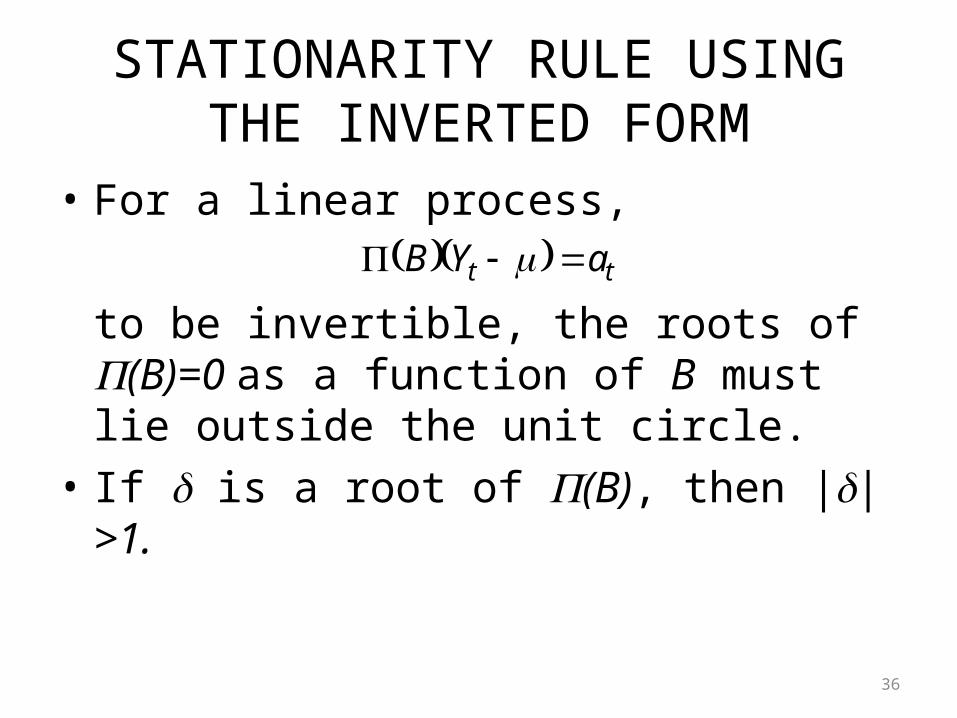
STATIONARITY RULE USING THE INVERTED FORM

• For a linear process,

to be invertible, the roots of (B)=0 as a function of B must lie outside the unit circle.

• If is a root of (B), then ||>1.

36

tt aYB

RANDOM SHOCK FORM AND INVERTED FORM

• AR and MA representations are not the model form. Because they contain infinite number of parameters that are impossible to estimate from a finite number of observations.

37

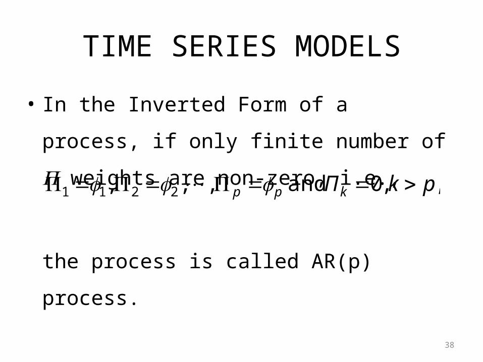
TIME SERIES MODELS

• In the Inverted Form of a process, if only finite

number of weights are non-zero, i.e.,

the process is called AR(p) process.

38

,,0 and ,,, 2211 pkΠkpp

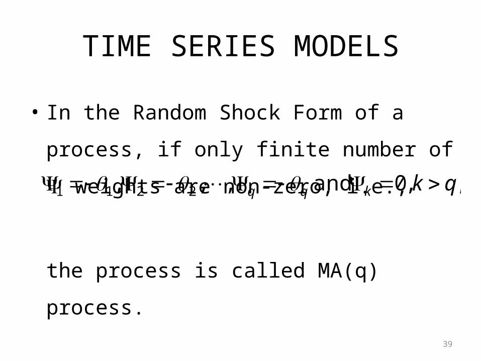
TIME SERIES MODELS

• In the Random Shock Form of a process, if only

finite number of weights are non-zero, i.e.,

the process is called MA(q) process.

39

,,0 and ,,, 2211 qkkqq

TIME SERIES MODELS

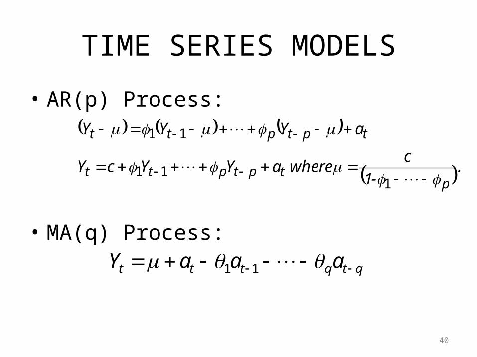
• AR(p) Process:

• MA(q) Process:

40

.-1

c whereaYYcY

aYYY

ptptptt

tptptt

111

11

.11 qtqttt aaaY

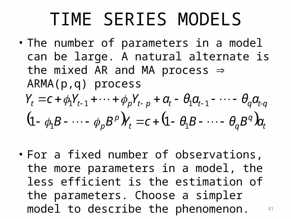
TIME SERIES MODELS• The number of parameters in a model can be

large. A natural alternate is the mixed AR and MA process ARMA(p,q) process

• For a fixed number of observations, the more parameters in a model, the less efficient is the estimation of the parameters. Choose a simpler model to describe the phenomenon.

41

tq

qtp

p

t-qqttptptt

aBθBθcYBB

aθaθaYYcY

11

1111

11