Chapter 4. Experimental set-up for wind tunnel tests

Chapter 4. Experimental set-up for wind tunnel tests

101


This chapter describes the boundary layer wind tunnel at the Ruhr-University Bochum,

the model of the Solar Updraft Tower and an outline of the tests. Moreover, the

preliminary results on the circular cylinder (without rings) are presented. Issues like

the influence of the Reynolds number and the choice of surface roughness are also

addressed in this chapter.

4.1 WiSt wind tunnel (Ruhr-University Bochum)

4.1.1 Geometry of the boundary layer wind tunnel

WiSt laboratory at Ruhr-University Bochum (Windingenieurwesen und

Strömungsmechanik http://www.ruhr-uni-bochum.de/wist) is an open circuit wind

tunnel with a total length of about 17 m. The tunnel itself has a length of 9.3 m. The

test section is 1.8 m in width and 1.6 m in height. In case of need, the upper ceiling of

the tunnel can be raised until 1.9 m. A turntable in the test section allows to test

different wind directions, if necessary. A honeycomb grid is located at the inlet of the

tunnel.

Figure 4.1 WiSt boundary layer wind tunnel at Ruhr-University Bochum

The turbulent boundary layer develops over a length of about 7.6 m. After a castellated

barrier having a maximum height of 425 mm, there are three turbulent generators of

1.5 m in height. They are built according to Counihan’s specifications (Counihan,

1969), as reported in the following sketch (Figure 4.2). The roughness field consists of

six panels with 36*36*36 mm3 cubes alternated to 36*36*18 mm

3 square prisms. It

creates the lowest and most important part of the boundary layer, which undergoes a

natural evolution along the wind tunnel and the largest eddy reaches approximately the


102

thickness of this surface layer, i.e. 30-40 cm. The turbulence in the upper layer is

created by turbulence generators. At a distance of about 3.5 times the height of the

turbulent generators, the two layers merge and continue to grow together. The

castellated barrier acts as an adjustment element. All these facilities (castellated

barrier, turbulence generators and roughness field) are removed in case of low-

turbulence tests in empty tunnel and approximately uniform flow. The boundary layer

at each wall affects a distance of about 30 cm.

2tan2

2

21

2

ϕxG

H

yHx

=

−=

Figure 4.2 Turbulent generators of Counihan type

The diffusor and the centrifugal fan are placed at the end of the wind tunnel. The

engine allows to attain a maximum wind speed of about 28-30 m/s with 1500 turns per

minute of the fan. A Prandtl tube allows to measure the dynamic pressure of the

incoming flow. Temperature sensors acquire temperature during the measurements. It

allows to calculate the air density and therefore the mean wind speed by applying

Bernoulli equation. The Prandtl tube is normally placed at 1.3 m in height – out of the

influence of the wall of the wind tunnel – but its position may change depending on

the tests.

Figure 4.3 View of the model in the wind tunnel with turbulent facilities


104

4.1.2 Flow characteristics

The castellated barrier, the turbulent generators and the roughness field, previously

described, produce a certain boundary layer namely RAU8. For the wind tunnel tests

on the solar tower, however, a slightly modified version of RAU8 is adopted, due to

the presence of the collector. It is named RAU8+collector (Figure 4.1). The collector,

i.e. a smooth panel of 4 m in length, centered at the tower position, was introduced

with the aim of creating a two-phase profile, as it should be expected in full-scale. Due

to the presence of the collector, the last roughness panel (the shortest one, 0.33 m in

length) had to be removed. The final set-up of the wind tunnel resulted like that:

Figure 4.4 View of the Solar Tower in the wind tunnel at the Ruhr-University Bochum

The ESDU Data Items 82026 allow to estimate the height of the internal layer which

develops after a roughness change, as that produced by the smooth collector roof. z0,1

and z0,2 are the roughness lengths corresponding to the upwind and downwind

conditions, respectively. Uz1 and Uz2 are the resulting wind profiles. At a certain

distance x from the step change in roughness, it can be assumed that the wind speed

profile consists of a lower portion (internal layer), where the velocity is dependent on

x and it is given by KxUz2, and an upper portion where the profile is the same as

upwind. The height of the internal layer, at which the two portions intersect, can be

estimated according to the ESDU procedure. If it is assumed that the smooth collector

has a surface roughness z0,2 = 0.005 m, while the upwind conditions are those

described in chapter 2 for the H&D model (Uz1(10m) = 25 m/s, z0,1 = 0.05 m, latitude

= 23°), an internal layer of approximately 200 m can be calculated in the full-scale

condition at a distance equal to the radius of the collector Rcoll (Table 4.1).


105

Table 4.1 Effect of a step change in roughness according to ESDU 82026

at the tower position

Upwind conditions

(full-scale)

Downwind conditions

(full-scale)

z01 0.05 m z02 0.005 m

u*1 1.898 m/s u*2 1.638 m/s

Internal layer height in m (full-scale) hi 201

Kx factor at x = Rcoll = 2000 m after the roughness change 0.9070

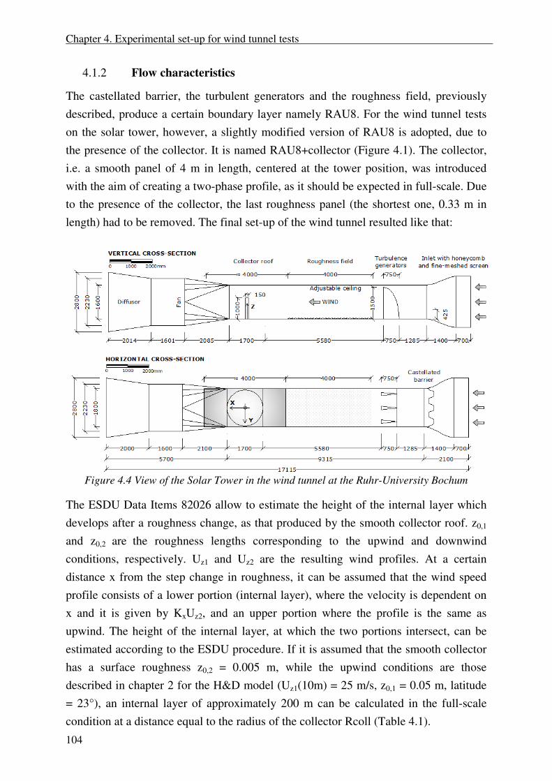
Instruments for velocity measurements

The velocity profile is measured with hot-wires anemometers. Cross wires allow to

measure two wind components (either u and v, or u and w). More than one probe can

record simultaneously in the wind tunnel; the Multichannel CTA 54N80 by Dantec is

an amplifier which allows to measure up to 16 channels. In the experiments, however,

only two cross-wire probes were used (four channels) plus temperature and Prandtl

velocity (two other channels). The A/D converter is the same as for pressure

measurements (see section 4.1.3) and it is set to a sampling frequency of 2 kHz.

a) b)

Figure 4.5 Miniature wires (X-array): a) during experiments; b) zoom

The multichannel CTA is designed for use with miniature wire probes (type 55P61-64)

in combination with 4m probe cables. Each channel of the CTA can be set to a certain

“decade resistance”, defined as twenty times the operating resistance. The latter

depends on the resistances of the sensor, of the probe support and of the probe cable.

The wires are 5 μm in diameter and 1.2 mm long. They are suspended between two

needle-shaped prongs. The frequency bandwidth is 10 kHz and filters can be applied.


106

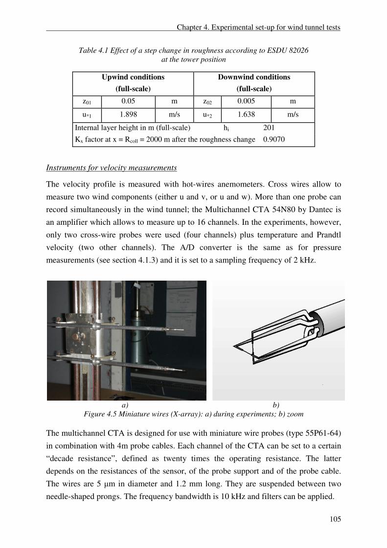
The anemometers are calibrated in laminar flow in the calibration tunnel. The

calibration establishes a relation between the CTA output (voltages) and the flow

velocity. It is performed by exposing the probe to a set of known velocities, U, and the

corresponding voltages E are recorded. A fitting curve through the points (E,U)

represents the transfer function to be used when converting data records from voltages

into velocities. The fitting curve which is adopted is a polynomial curve of 4th

order

(equation (4.1)). The coefficients are calculated by fitting the data in the least-squares

sense. An example reported is in Figure 4.6.

Figure 4.6 Calibration curve – wires a and b of one probe (experiment 24.10.2011)

44

33

2210

ECECECECCU ++++= (4.1)

If the temperature varies during calibration and the experiment, the recorded voltages

must be corrected (Ecorr) with the formula:

aE

aT

wT

Tw

T

corrE

5.0

0

−

−= (4.2)

where: Ea = acquired voltage; Tw = sensor hot temperature = 250°; T0 = ambient

reference temperature (during calibration); Ta = ambient temperature during

acquisition. The expression can be used for moderate temperature changes in air (±

5°C). The useful range may be expanded (Jørgensen Finn E., 2002) by reducing the

exponent from 0.5 to 0.4 or 0.3.


107

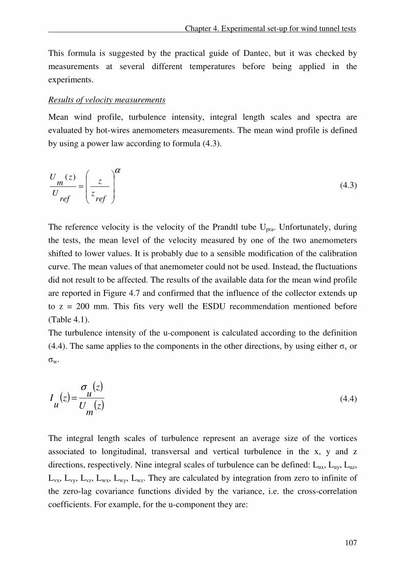
This formula is suggested by the practical guide of Dantec, but it was checked by

measurements at several different temperatures before being applied in the

experiments.

Results of velocity measurements

Mean wind profile, turbulence intensity, integral length scales and spectra are

evaluated by hot-wires anemometers measurements. The mean wind profile is defined

by using a power law according to formula (4.3).

α

=

refz

z

refU

zm

U )( (4.3)

The reference velocity is the velocity of the Prandtl tube Upra. Unfortunately, during

the tests, the mean level of the velocity measured by one of the two anemometers

shifted to lower values. It is probably due to a sensible modification of the calibration

curve. The mean values of that anemometer could not be used. Instead, the fluctuations

did not result to be affected. The results of the available data for the mean wind profile

are reported in Figure 4.7 and confirmed that the influence of the collector extends up

to z = 200 mm. This fits very well the ESDU recommendation mentioned before

(Table 4.1).

The turbulence intensity of the u-component is calculated according to the definition

(4.4). The same applies to the components in the other directions, by using either σv or

σw.

( )( )

( )zm

U

zuz

uI

σ= (4.4)

The integral length scales of turbulence represent an average size of the vortices

associated to longitudinal, transversal and vertical turbulence in the x, y and z

directions, respectively. Nine integral scales of turbulence can be defined: Lux, Luy, Luz,

Lvx, Lvy, Lvz, Lwx, Lwy, Lwz. They are calculated by integration from zero to infinite of

the zero-lag covariance functions divided by the variance, i.e. the cross-correlation

coefficients. For example, for the u-component they are:


108

( ) ( ) xdxu

xdxu

R

u

uxL ∆∫

∞+∆=∆∫

∞+∆=

0

0,

0

0,2

1ρ

σ

(4.5)

( ) ( ) ydyu

ydyu

R

u

uyL ∆∫

∞+∆=∆∫

∞+∆=

0

0,

0

0,2

1ρ

σ

(4.6)

( ) ( ) zdzu

zdzu

R

u

uzL ∆∫

∞+∆=∆∫

∞+∆=

0

0,

0

0,2

1ρ

σ

(4.7)

The integral length scale Lux can be easily calculated by Taylor’s hypothesis, which

allows to use only one signal measured in one position, by assuming that the vortices

move in the along-wind direction at the mean wind speed:

uxT

mU

uxL = (4.8)

Tux is the integral time scale, i.e. the integral of the auto-correlation function from zero

until infinite (equation (4.9)). In practical terms, the integration can be extended until

the first zero crossing, because all the following ondulations of the auto-correlation

coefficient approximately average to zero. Also other methods exist, for example the

exponential method, which assumes that the auto-correlation function has an

exponential decay (Schrader, 1993). Alternately, Tux can also be calculated by fitting

the spectrum of the signal with an analytical expression of the velocity spectrum (e.g.

von Karman spectrum in isotropic flow).

( )∫∞

=

0

ττρ duxxu

T (4.9)

Besides Lux, for the purpose of this work it is especially important to investigate the

integral length scale of the u-component in the z direction, i.e. Luz. Approximately, in

the atmospheric boundary layer flow, it is one half of Lux, apart from very close to the

ground. In this work, Luz is calculated at each height by integration of the cross-

correlation coefficients from zero until infinite (equation (4.10)). This requires

simultaneous measurements of wind velocity in at least two points (Figure 4.5).


109

∫∞

∆

∆=

∆

0

,, zdzref

zu

zref

zzu

L ρ (4.10)

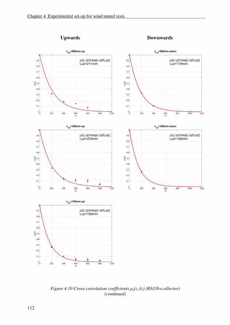
Vertical cross-correlations of the u-component in the undisturbed flow are measured

both upwards and downwards at the following reference heights: 100-300-500-700-

900-1100 mm. They are fitted with a negative exponential function, from which Luz is

easily derived:

( ) Luz

z

ezu

∆−

=∆ρ (4.11)

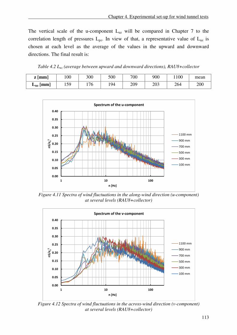
The spectra of the u and v components are reported in Figure 4.11 and Figure 4.12. In

particular, the investigation of the cross-wind component (v) of the wind velocity is

important for a deeper study of pressure fluctuations at the flanges of the cylinder and

for transversal oscillations of the structure in a dynamic calculation. The spectrum of

the v-component, compared to the spectrum of the u-component, appears to be shifted

(Figure 4.13). It implies higher energy in the cross-wind direction at relatively high

frequency, i.e. in the frequency range of most of structures sensitive to wind.

Figure 4.7 Mean wind profile (RAU8+collector)

y = 0.2832x0.1719

y = 0.3625x0.1296

0.1

1

10 100 1000

Um

(z)/

Up

ra

z [mm]

RAU8+collector [24.10.2011, 1400-1,2,3]

z >= 200

z < 200

0

200

400

600

800

1000

1200

1400

1600

0 0.2 0.4 0.6 0.8 1

z [m

m]

Um(z)/Upra

RAU8+collector [24.10.2011, 1400-1,2,3]

INFLUENCE

OF THE

COLLECTOR


110

Figure 4.8 Turbulence intensity (RAU8+collector and RAU8)

Figure 4.9 Integral length scale, Lux (RAU8+collector) in the figure: first zero-crossing

0

100

200

300

400

500

600

700

800

900

1000

1100

1200

1300

1400

1500

1600

0.00 0.05 0.10 0.15 0.20

z [m

m]

Iu

RAU8+collector&RAU8 [24.10.2011+13.12.2011]

RAU8

RAU8+coll.


111

Upwards

Downwards

Figure 4.10 Cross-correlation coefficients ρu(z,Δz) (RAU8+collector)

(continued in the next page)


112

Upwards

Downwards

Figure 4.10 Cross-correlation coefficients ρu(z,Δz) (RAU8+collector)

(continued)


113

The vertical scale of the u-component Luz will be compared in Chapter 7 to the

correlation length of pressures Lpz. In view of that, a representative value of Luz is

chosen at each level as the average of the values in the upward and downward

directions. The final result is:

Table 4.2 Luz (average between upward and downward directions), RAU8+collector

z [mm] 100 300 500 700 900 1100 mean

Luz [mm] 159 176 194 209 203 264 200

Figure 4.11 Spectra of wind fluctuations in the along-wind direction (u-component)

at several levels (RAU8+collector)

Figure 4.12 Spectra of wind fluctuations in the across-wind direction (v-component)

at several levels (RAU8+collector)

0.00

0.05

0.10

0.15

0.20

0.25

0.30

0.35

0.40

1 10 100

nS

/σu

2

n [Hz]

Spectrum of the u-component

1100 mm

900 mm

700 mm

500 mm

300 mm

100 mm

0.00

0.05

0.10

0.15

0.20

0.25

0.30

0.35

0.40

1 10 100

nS

/σu

2

n [Hz]

Spectrum of the v-component

1100 mm

900 mm

700 mm

500 mm

300 mm

100 mm


114

Figure 4.13 Spectra of wind fluctuations in the along-wind (u-component) and across-wind

(v-component) directions at 500 mm (RAU8+collector)

The unusual peak at about 3-4 Hz in the u-spectrum in Figure 4.13 (detectable at

higher frequencies also in the v-spectrum) is not produced by the slight modification

of RAU8 by including the collector. It is difficult to find its precise cause. By the way,

it is also recorded in pressure measurements. Once pressures are integrated along the

circumference, for example to calculate the lift force, such a peak disappears in the lift

spectrum because the two half lifts have negative correlation in that range of

frequencies.

In any case, flow disturbances are not surprising in a wind tunnel. They can be

produced by the rotor blades, the motor itself, the vibrations of the ground surface and

of the wind tunnel walls or they can be electrical disturbances.

The similarity criteria between wind tunnel and full-scale require that the

dimensionless parameters (e.g. St, Re, Iu,…) assume the same value in the wind tunnel

and in full-scale. All the quantities which have the same dimension (for example,

length, velocity or time) should be scaled according to the length scale λL, λV, λT,

respectively. They represent the ratios between the values in the wind tunnel and the

values in full-scale.

Due to the scale of the model, it is not possible in this work to reproduce in the wind

tunnel the same Re as in full-scale. Its effects and the use of surface roughness in order

to overcome the mismatch are discussed in section 4.4. The similarity of St requires

that: λL = λV * λT.

0.00

0.05

0.10

0.15

0.20

0.25

0.30

0.35

0.40

1 10 100

nS

/σu

2

n [Hz]

Spectra of the u and v components at z = 500 mm

u-500mm

v-500mm


115

FSU

nD

WTU

nD

tS

=

= →

TVLλλλ *= (4.12)

If λL is equal to the scale of the model, i.e. 1:1000, the turbulence (in particular Lux)

and the boundary layer should be scaled accordingly. In fact, the full-scale value of Lux

is an uncertain parameter in itself. Chapter 2 proved that different codes and

calculation methods provide more or less similar results in the surface layer, but very

different ones in the Ekman layer. Similarly, Tux can be directly calculated from wind

tunnel data by equation (4.9); in full-scale it can be derived by Taylor hypothesis. The

comparison between Lux (Tux ) in the wind tunnel and in full-scale provides an

estimation of the approximation, in case the data are used in a structural calculation on

1-km prototype. In any case, Figure 4.14 shows that the turbulence scale reproduced in

the wind tunnel, multiplied by the scale factor 1000 (λL = 1:1000) is not too far from

the Code predictions (even extrapolated at large heights). Instead, the H&D model

would suggest much larger integral length scales, which cannot be reproduced in the

wind tunnel. This partial simulation of turbulence implies, with regard to the H&D

model, a smaller background response and higher dynamic amplification.

In conclusion, by assuming λL = 1:1000 and having λV = 1:2.05 (UFS(z=H) = 51.31

m/s; UWT (z=H) = 25.07 m/s), it results λF = 1/488; λT = 488. By looking at Figure 4.14

it can be inferred that it is not too far from the time scale that would be obtained by

comparing Tux in the wind tunnel and Tux in full-scale.

Figure 4.14 Integral length scale of turbulence Lux in full-scale. The violet marks represent

Lux in the wind tunnel divided by the length scale factor 1:1000.

0

100

200

300

400

500

600

700

800

900

1000

0 500 1000 1500

z [m

]

Lux [m]

Lux in full-scale (λL = 1:1000)

Eurocode

DIN EN

H&D

WT/λL


116

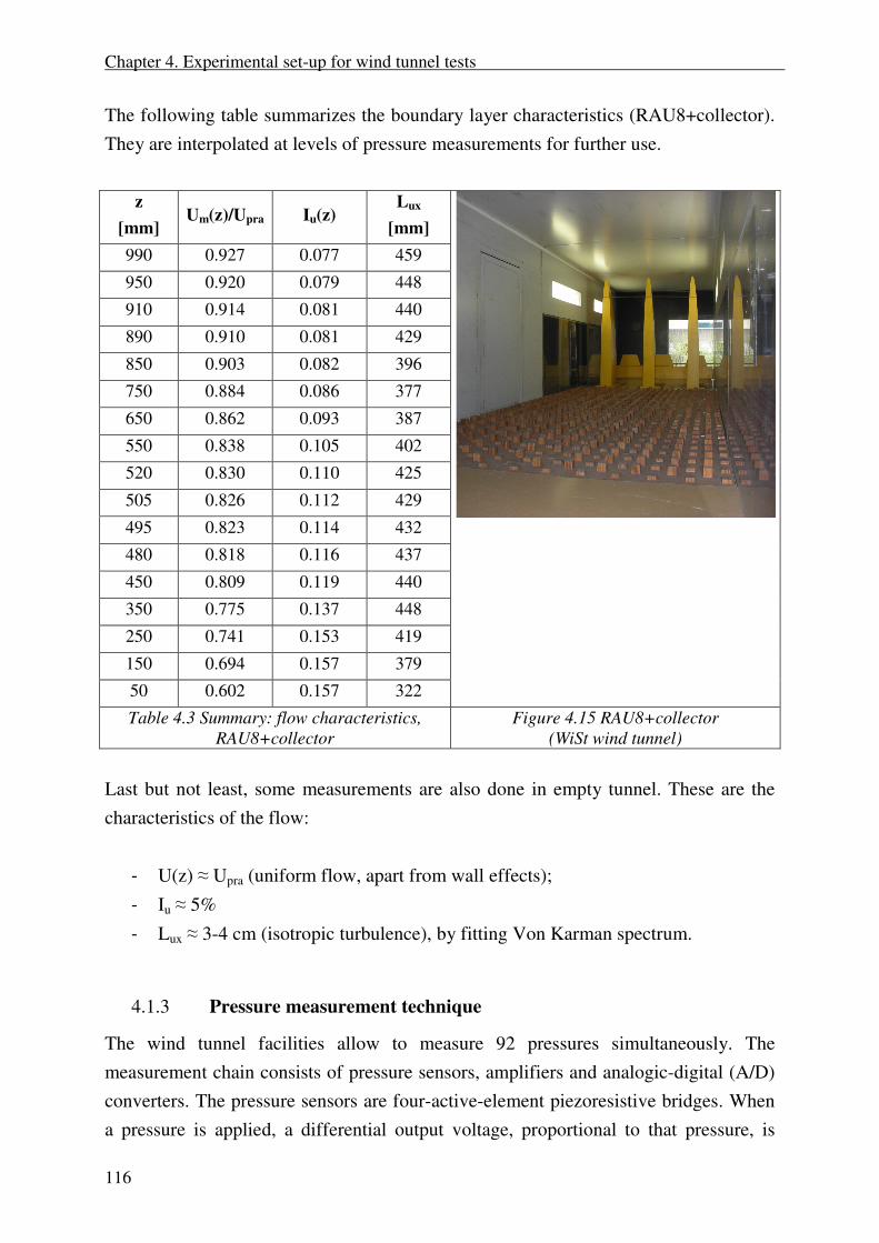
The following table summarizes the boundary layer characteristics (RAU8+collector).

They are interpolated at levels of pressure measurements for further use.

z

[mm] Um(z)/Upra Iu(z)

Lux

[mm]

990 0.927 0.077 459

950 0.920 0.079 448

910 0.914 0.081 440

890 0.910 0.081 429

850 0.903 0.082 396

750 0.884 0.086 377

650 0.862 0.093 387

550 0.838 0.105 402

520 0.830 0.110 425

505 0.826 0.112 429

495 0.823 0.114 432

480 0.818 0.116 437

450 0.809 0.119 440

350 0.775 0.137 448

250 0.741 0.153 419

150 0.694 0.157 379

50 0.602 0.157 322

Table 4.3 Summary: flow characteristics,

RAU8+collector

Figure 4.15 RAU8+collector

(WiSt wind tunnel)

Last but not least, some measurements are also done in empty tunnel. These are the

characteristics of the flow:

- U(z) ≈ Upra (uniform flow, apart from wall effects);

- Iu ≈ 5%

- Lux ≈ 3-4 cm (isotropic turbulence), by fitting Von Karman spectrum.

4.1.3 Pressure measurement technique

The wind tunnel facilities allow to measure 92 pressures simultaneously. The

measurement chain consists of pressure sensors, amplifiers and analogic-digital (A/D)

converters. The pressure sensors are four-active-element piezoresistive bridges. When

a pressure is applied, a differential output voltage, proportional to that pressure, is


117

produced. Differential sensors provide a differential voltage proportional to the

pressure differential between two ports. One port measures the wind pressure on the

model, the other one is connected to the static pressure of the Prandtl tube. Two

different pressure sensors are used:

- Type 1: Honeywell 170 PC

Measurement range ± 35 mbar

- Type 2: AMSYS 5812-0001-D-B

Measurement range ± 10.34 mbar

They are calibrated by using different factors, so that 5 mbar corresponds to 5 V for

the type 1 (the most sensitive) and 5 mbar corresponds to 1 volt for type 2. A static

calibration is performed to find pressure to voltage relations for each pressure sensor

by using a Betz manometer, which allows to load the system with a known pressure.

Figure 4.16 Pressure sensor Honeywell 170PC

Figure 4.17 Pressure cell AMSYS


118

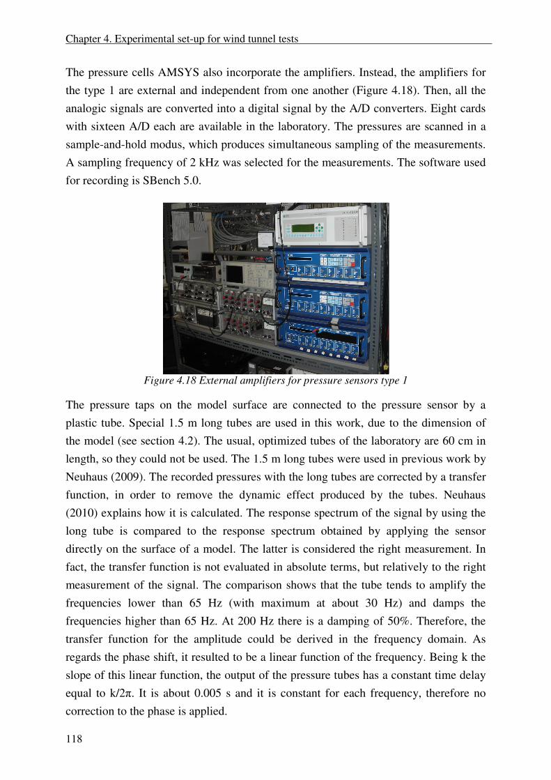
The pressure cells AMSYS also incorporate the amplifiers. Instead, the amplifiers for

the type 1 are external and independent from one another (Figure 4.18). Then, all the

analogic signals are converted into a digital signal by the A/D converters. Eight cards

with sixteen A/D each are available in the laboratory. The pressures are scanned in a

sample-and-hold modus, which produces simultaneous sampling of the measurements.

A sampling frequency of 2 kHz was selected for the measurements. The software used

for recording is SBench 5.0.

Figure 4.18 External amplifiers for pressure sensors type 1

The pressure taps on the model surface are connected to the pressure sensor by a

plastic tube. Special 1.5 m long tubes are used in this work, due to the dimension of

the model (see section 4.2). The usual, optimized tubes of the laboratory are 60 cm in

length, so they could not be used. The 1.5 m long tubes were used in previous work by

Neuhaus (2009). The recorded pressures with the long tubes are corrected by a transfer

function, in order to remove the dynamic effect produced by the tubes. Neuhaus

(2010) explains how it is calculated. The response spectrum of the signal by using the

long tube is compared to the response spectrum obtained by applying the sensor

directly on the surface of a model. The latter is considered the right measurement. In

fact, the transfer function is not evaluated in absolute terms, but relatively to the right

measurement of the signal. The comparison shows that the tube tends to amplify the

frequencies lower than 65 Hz (with maximum at about 30 Hz) and damps the

frequencies higher than 65 Hz. At 200 Hz there is a damping of 50%. Therefore, the

transfer function for the amplitude could be derived in the frequency domain. As

regards the phase shift, it resulted to be a linear function of the frequency. Being k the

slope of this linear function, the output of the pressure tubes has a constant time delay

equal to k/2π. It is about 0.005 s and it is constant for each frequency, therefore no

correction to the phase is applied.


119

The effective range in which the digital filter applied to the pressure corrects the signal

is up to 200 Hz. Therefore, even if the sampling frequency is 2000 Hz, 200 Hz is the

cut-off frequency. After that, the frequencies are damped. The reason for which such a

high sampling frequency was chosen, despite the relatively lower cut-off frequency, is

the higher accuracy in the time domain even for high-frequency (e.g. 200 Hz)

fluctuations.

The time histories of pressures are acquired for a duration of N/fsampl = 218

/2000 =

131.072 s. 218

is the number of time steps (N) in each recorded signal.

4.2 Model of the solar updraft tower

The model of the Solar Updraft Tower for wind tunnel tests is a circular cylinder of 1

m in height and 15 cm in diameter, made of plexiglass. The aspect ratio is about 1:7

(H/D = 6.7). The dimensions of the model are chosen in order not to have a too high

blockage ratio. On the transversal plane the model occupies an area of 1*0.15m = 0.15

m2, while the wind tunnel cross-section is 1.8*1.6m = 2.88 m

2. The ratio between the

two values gives a blockage of 5%, which can be accepted without any correction of

results. In scale 1:1000, the model represents a 1-km tall prototype.

Figure 4.19 Wind tunnel model of the Solar Tower


120

Even though the real shape of the tower, according to the pre-designs mentioned in

Chapter 1, may turn into a hyperboloid at lower levels, the wind tunnel model is a

circular cylinder. This shape, which simplified the manufacturing, allows to evaluate

the aerodynamic effects without any loss in generality. Moreover, the model is rigid

and in order to avoid vibrations two wires3 at 800 mm fix it at the wall of the wind

tunnel.The tower model is equipped with 342 pressure taps, placed at several levels

along the height and in the circumferential direction, in order to investigate vertical

and horizontal cross-correlations. Both external and internal pressures are measured at

each level. The external pressure taps are placed at 17 levels (990-950-910-890-850-

750-650-550-520-505-495-480-450-350-250-150-50 mm) at an angular distance of

20° (≈ 26 mm) at each level. The internal pressure taps in the tip region are 9 per level

(angular distance = 45°) at 990 and 950 mm. Along the height (at 850-750-650-550-

520-450-350-250-150-50 mm) they are 2 per level, at 0° and 180°. This is better

shown in the drawing of the model (Drawing 2 on page 125).

The wind tunnel scale of the model and of the boundary layer properties reduces by

around three orders of magnitude the Reynolds number from full-scale to wind tunnel

conditions (Re = UD/ν; Re,FS ≈ 50*150/1.5*10-5

= 5*108; Re,WT ≈ 30*0.15/1.5*10

-5 =

3*105). Because of that, surface roughness (ribs) is applied along the model, in order

to reproduce the same state of the flow as in full-scale. The target condition is

described in the VGB guideline for cooling towers (curves K1.5-1.6). The final choice

for the surface roughness – as it will be proved in section 4.4 – is ks/D =

0.25mm/150mm, being k the thickness of the ribs. The ribs are at an angular distance

of 20°, i.e. in between two pressure taps (Figure 4.20). In any case, ribs are only

applied in the scaled wind tunnel model because of Re effects, while the surface of the

tower in full-scale conditions must be smooth in order to reduce the drag (Figure 3.10,

Niemann,2009) .

The collector roof (4 km in diameter in full-scale) is also modeled in the wind tunnel.

It is a very smooth panel in HDF, ideally representing the smooth glass surface

encountered by the incoming wind (Figure 4.4). Its function in the wind tunnel is only

the creation of a two-phase wind profile. The efflux inside the tower is not reproduced

by means of the collector, but artificially by using the pressure difference outside-

inside the wind tunnel. In fact, one of the major difficulties in the design of the model

was the creation of the efflux inside the tower, due to the presence of 342 tubes inside

the cylinder, which connect each measuring point on the shell to the pressure

3 The wires are too thin to modify the flow condition and disturb the measurements.


121

transducers. The presence of such a large number of tubes inside the tower would

affect the internal flow. Moreover, the efflux had to be created somehow.

After having discussed several possibilities, it was decided to use a second circular

cylinder, having a smaller diameter, to be placed inside the main cylinder representing

the tower. This configuration of a pipe in a pipe allows placing all the tubes for

measuring the pressures in the small cavity between the two cylinders. The two

cylinders are glued together at the top through a union ring, as it can be seen in Figure

4.20.

Figure 4.20 Tube-in-a-tube solution.

The outer cylinder is shorter in length than the inner one, so that the pressure tubes can

come out of the model (below the wind tunnel) when the outer cylinder ends. As said,

the efflux inside the tower is created by the pressure difference inside-outside the wind

tunnel. In addition, a ventilator is placed below the model - at the opening of the inner

cylinder - in order to achieve higher efflux velocities, if needed. Below the ventilator

there is a moving plate which allows to regulate the opening, so to achieve the desired

air capacity for the efflux. In addition, tests are also made in no-efflux conditions

(outage condition), by closing the opening below the ventilator. Even though in reality

the value of the efflux velocity during operation of the power plant depends on several

conditions (e.g. the temperature rise in the collector, the pressure drop at the turbines


122

etc.), a quite realistic condition for the design is achieved in the wind tunnel when the

velocity of the efflux inside the tower is around one half of the wind tunnel velocity.

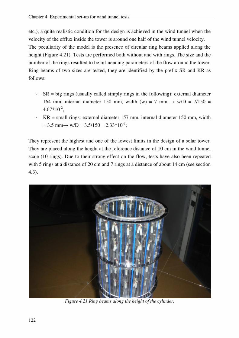
The peculiarity of the model is the presence of circular ring beams applied along the

height (Figure 4.21). Tests are performed both without and with rings. The size and the

number of the rings resulted to be influencing parameters of the flow around the tower.

Ring beams of two sizes are tested, they are identified by the prefix SR and KR as

follows:

- SR = big rings (usually called simply rings in the following): external diameter

164 mm, internal diameter 150 mm, width (w) = 7 mm → w/D = 7/150 =

4.67*10-2

;

- KR = small rings: external diameter 157 mm, internal diameter 150 mm, width

= 3.5 mm→ w/D = 3.5/150 = 2.33*10-2

;

They represent the highest and one of the lowest limits in the design of a solar tower.

They are placed along the height at the reference distance of 10 cm in the wind tunnel

scale (10 rings). Due to their strong effect on the flow, tests have also been repeated

with 5 rings at a distance of 20 cm and 7 rings at a distance of about 14 cm (see section

4.3).

Figure 4.21 Ring beams along the height of the cylinder.


123

Figure 4.22 The support system for installation

Figure 4.23 Complete installation


124

a)

b)

c)

d)

e)

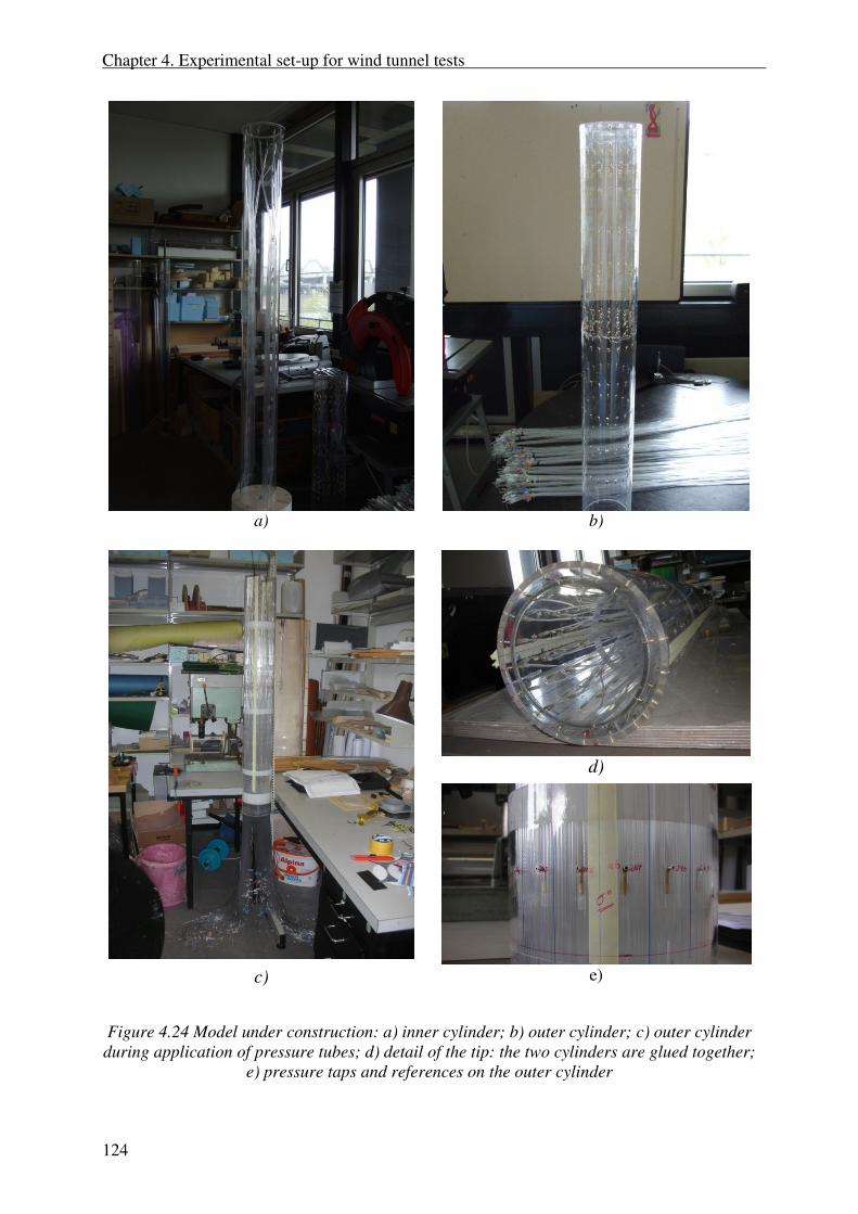
Figure 4.24 Model under construction: a) inner cylinder; b) outer cylinder; c) outer cylinder

during application of pressure tubes; d) detail of the tip: the two cylinders are glued together;

e) pressure taps and references on the outer cylinder


127

4.3 Outline of the experiments

The model of the tower without rings is the reference case to identify the flow

condition and study the aerodynamic of the flow around a circular cylinder H/D = 7,

immersed in boundary layer flow. Most of the studies in literature refer to sub-critical

Re; in addition, the aspect ratio and the characteristics of the boundary layer influence

the results (Chapter 3). Therefore, before investigating the effect of the ring beams, it

is necessary to have a deep knowledge of the flow around the circular cylinder without

ring beams. Because of that, each test is always made twice: once with the rings, once

without them. In addition, several conditions, in terms of surface roughness, flow

velocity, boundary layer, efflux, number of rings, size of rings are tested. The

nomenclature used in the campaign is described in the following:

1. Boundary layer:

- T1 = boundary layer flow RAU8 + collector;

- T3 = uniform flow (empty tunnel);

2. Surface roughness conditions on the outer surface of the model:

- R0 = smooth cylinder;

- R1 = ribs at a spacing of 20°, ks = 0.250 mm (ks/D = 1.67*10-3

);


);


);


);


);

The surface roughness is always made of ribs. This choice is motivated by

simplicity of manufacturing and consolidated experience on cooling towers

(VGB, 2010).

3. Wind tunnel velocity: for practical reasons, the wind tunnel velocity to be used

in each test is identified by the number of rounds per minute (rpm) of the fan.

Depending on the static pressure and on the temperature during measurements,

the density of air and consequently the velocity may change. A small difference

in the measured velocity corresponding to the same rpm is also noted in

presence or absence of boundary layer (RAU8 or empty tunnel) and in presence

or absence of efflux in the chimney. Approximately, it results:

- 100 rpm; Upra ≈ 3 m/s

- 200 rpm; Upra ≈ 5 m/s


128

- 400 rpm; Upra ≈ 8 m/s

- 600 rpm; Upra ≈ 12 m/s

- 800 rpm; Upra ≈ 16 m/s

- 1000 rpm; Upra ≈ 20 m/s

- 1250 rpm; Upra ≈ 25 m/s

- 1400 rpm; Upra ≈ 27 m/s

1400 rpm is the highest velocity which was used, although the capacity of the

wind tunnel was even higher, up to 1500 rpm. However, the resulting pressure

at higher wind speed would have exceeded the sensitivity range of the pressure

transducers type 2, which could not be regulated.

The low velocity range 100-200-400 rpm is tested only on the smooth cylinder,

in the hope to reach subcritical conditions (laminar separation). However, at

very low speed the wind tunnel velocity was not always stable.

4. Efflux condition:

- EF0 = no efflux;

- EF1 = efflux;

The velocity of the efflux is regulated at about one half of the wind tunnel

velocity (section 4.4.1).

5. Effect of ring beams:

- SR0 = no rings;

- SR1 = ten big rings along the height, equally spaced at a distance of 10

cm;

- SR7 = seven big rings along the height, equally spaced at a distance of

14 cm (15 cm in the two lowest compartment);

- SR5 = five big rings along the height, equally spaced at a distance of 20

cm;

- KR1 = ten small rings along the height, equally spaced at a distance of

10 cm;

- KR7 = seven small rings along the height, equally spaced at a distance of

14 cm (15 cm in the two lowest compartment);

- KR5 = five small rings along the height, equally spaced at a distance of

20 cm;


129

The wind tunnel equipment allows to measure maximum 92 pressures simultaneously.

However, some sensors where out of use at the time of the tests, therefore no more

than four levels (with 18 pressure taps each, on the external surface) could be

measured at the same time, plus other positions at proper convenience. In the first plan

of the experiments, it was decided to measure all the correlations of the 342 pressure

taps in the basic conditions: T1(&T3)-SR0&SR1-EF0(&EF1)-R1, where the

nomenclature out of brackets had the priority. In order to measure all the cross-

correlation, the pressures had to be divided into groups and each group had to be

measured with all the other ones. However, due to the appearance of the new

phenomenon described in Chapter 5 – during the second set of measurements (May

2011) – the original plan of experiments was revised. Different experimental

conditions had to be tested for a deeper understanding of the phenomenon: not only

SR0 and SR1, but also SR5, SR7, KR1, KR5, KR7; not only R1, but also R0-R2-R3-

R4-R5. Consequently, the complete correlation field could not be measured, but only

the most important pressures were measured simultaneously.

In summary, the following series of measurements were defined (only pressures on

external surface and complete circumference are mentioned):

- MS01: levels z = 990-950-910-890 mm;

- MS02: levels z = 910-890-850-750 mm;

- MS03: levels z = 750-650-550 mm;

- MS04: levels z = 550-520-505-495 mm;

- MS05: levels z = 505-495-480-450 mm;

- MS06: levels z = 450-350-250-150 mm;

- MS07: levels z = 250-150-50 mm + vertical at 0°;

- MS08: levels z = 990-950-750 mm;

- MS09: levels z = 550-450 mm;

- MS10: levels z = 450-50 mm + vertical at 80°;

- MS28: verticals at 20°, 120°, 180°, 300°;

- MS30/MS32: levels z = 950-850-750-650 mm;

- MS31: levels z = 950, 890, 750, 650 mm;

- MS33: levels z = 950-910-890-850 mm;

- MS34: levels z = 650-550-520-480 mm;

The experimental campaign was articulated in the following four sets, which became

necessary as the investigation was proceeding:


130

Set n.1 (April 2011):

Turbulence setting: T1

Rings: SR0

Efflux: EF0/EF1

Surface roughness: R1

Wind tunnel velocity (rpm): 600/800/1000/1250/1400

Measurement series: MS01/02/03/04/05/06/07/08/09/10/28;

Set n.2 (May 2011):


Rings: SR0/SR1

Efflux: EF0/EF1

Surface roughness: R1

Wind tunnel velocity (rpm): 0600/0800/1000/1100/1250/1400

Measurement series: MS01/02/04/05/08/09;

Set n.3 (October 2011):


Rings: SR0/SR1/SR7/SR5/KR1/KR7/KR5

Efflux: EF0/EF1

Surface roughness: R0/R1/R2/R3/R4/R5


Measurement series: MS30/31;

Set n.4 (December 2011):


Rings: SR0/SR1

Efflux: EF0/EF1

Surface roughness: R1/R3


Measurement series: MS32/33/34;


131

4.4 Preliminary results on the circular cylinder

In this section, preliminary results on the cylinder without rings are presented.

4.4.1 Velocity of efflux

The tests are performed in two conditions: open efflux (EF1) and closed efflux (EF0).

The latter represents the condition of out of use of the power plant. For many aspects,

EF0 is more dangerous than EF1. In particular, the tip effect in EF0 is stronger. In the

condition of open efflux, the tests are performed with only one efflux velocity. The

influence of different efflux velocities on the pressures is not investigated. The efflux

velocity which acts in EF1 is around one half of the undisturbed flow velocity (Upra).

This is achieved in the experiments by defining a proper opening below the model,

through the position of the wooden plate under the ventilator (Figure 4.23).

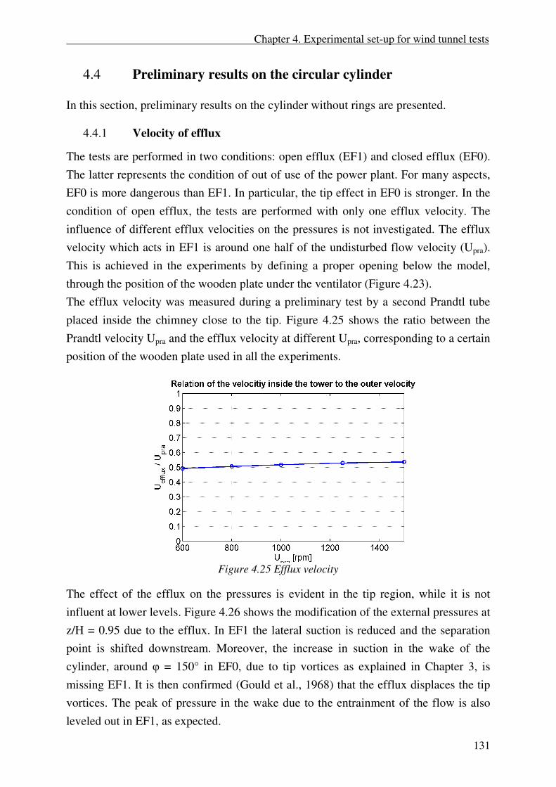
The efflux velocity was measured during a preliminary test by a second Prandtl tube

placed inside the chimney close to the tip. Figure 4.25 shows the ratio between the

Prandtl velocity Upra and the efflux velocity at different Upra, corresponding to a certain

position of the wooden plate used in all the experiments.

Figure 4.25 Efflux velocity

The effect of the efflux on the pressures is evident in the tip region, while it is not

influent at lower levels. Figure 4.26 shows the modification of the external pressures at

z/H = 0.95 due to the efflux. In EF1 the lateral suction is reduced and the separation

point is shifted downstream. Moreover, the increase in suction in the wake of the

cylinder, around φ = 150° in EF0, due to tip vortices as explained in Chapter 3, is

missing EF1. It is then confirmed (Gould et al., 1968) that the efflux displaces the tip

vortices. The peak of pressure in the wake due to the entrainment of the flow is also

leveled out in EF1, as expected.


132

Figure 4.26 Cp,m and Cp,σ in the tip region (z/H = 0.95): influence of efflux.

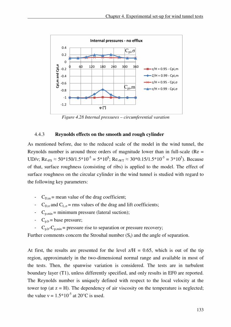
4.4.2 Internal pressure

The internal pressure coefficient Cpi is calculated with reference to the velocity

pressure at z = H. The pressure coefficient is higher is case of efflux, both in the mean

as well as in the rms. Its value is approximately constant along the height and along

the circumference. Only close to the tip it exhibits some variation. In any case, the

value of Cpi is lower than the typical value for cooling towers (Cpi = -0.5 in VGB,

2010).

Figure 4.27 Internal pressures – spanwise varation

In absence of efflux, the internal pressure is somewhat higher at z/H = 0.99, φ = 180°,

probably due to an entrainment of fluid inside the cylinder (Figure 4.28). However, the

level z/H = 0.95 is already unaffected and the internal pressure does not show any

circumferential variation.

-2

-1.5

-1

-0.5

0

0.5

1

0 30 60 90 120 150 180 210 240 270 300 330 360C

p,m

an

d C

p,σ

φ [°]

z/H = 0.95

EF0

EF1

0

0.1

0.2

0.3

0.4

0.5

0.6

0.7

0.8

0.9

1

-1.5 -1 -0.5 0 0.5

z/H

Cpi,m and Cpi,σ

Internal pressures - with/without efflux

EF0 Cpi,m(0°)

EF0 Cpi,σ(0°)

EF1 Cpi,m(0°)

EF1 Cpi,σ(0°)


133

Figure 4.28 Internal pressures – circumferential varation

4.4.3 Reynolds effects on the smooth and rough cylinder

As mentioned before, due to the reduced scale of the model in the wind tunnel, the

Reynolds number is around three orders of magnitude lower than in full-scale (Re =

UD/ν; Re,FS ≈ 50*150/1.5*10-5

= 5*108; Re,WT ≈ 30*0.15/1.5*10

-5 = 3*10

5). Because

of that, surface roughness (consisting of ribs) is applied to the model. The effect of

surface roughness on the circular cylinder in the wind tunnel is studied with regard to

the following key parameters:

- CD,m = mean value of the drag coefficient;

- CD,σ and CL,σ = rms values of the drag and lift coefficients;

- Cp,min = minimum pressure (lateral suction);

- Cp,b = base pressure;

- Cp,b-Cp,min = pressure rise to separation or pressure recovery;

Further comments concern the Strouhal number (St) and the angle of separation.

At first, the results are presented for the level z/H = 0.65, which is out of the tip

region, approximately in the two-dimensional normal range and available in most of

the tests. Then, the spanwise variation is considered. The tests are in turbulent

boundary layer (T1), unless differently specified, and only results in EF0 are reported.

The Reynolds number is uniquely defined with respect to the local velocity at the

tower top (at z = H). The dependency of air viscosity on the temperature is neglected;

the value ν = 1.5*10-5

at 20°C is used.

-1.2

-1

-0.8

-0.6

-0.4

-0.2

0

0.2

0.4

0 60 120 180 240 300 360

Cp

i,m

an

d C

pi,

σ

φ [°]

Internal pressures - no efflux

z/H = 0.95 - Cpi,m

Z/H = 0.99 - Cpi,m

z/H = 0.95 - Cpi,σ

z/H = 0.99 - Cpi,σCpi,m

Cpi,σ


134

Figure 4.29 plots the drag coefficient distribution at z/H = 0.65 for different Reynolds

numbers (i.e. different wind tunnel velocities) and for different surface roughness

conditions. The blue curve (R0) refers to the smooth cylinder (according to the

nomenclature in section 4.3). It can be seen that the flow around the smooth cylinder is

at first in the critical state, characterized by the fall of CD until the minimum at Recr ≈

1.9*105. After that, the horizontal plateau is typical of the supercritical range for

smooth cylinders, according to Roshko’s classification (Chapter 3). On the rough

cylinder in turbulent boundary layer flow (T1), for any type of surface roughness (R1-

R5) the state of the flow is already beyond the critical Re. This is not only due to the

surface roughness, but it is also enhanced by the turbulence of the flow. In fact, it is

interesting to compare these results to the black dashed line in the figure, which is the

only one referring to uniform flow and lower Iu (empty tunnel). However, due to lack

of data, it is at z/H = 0.55. In any case, it can be seen that at high (effective) Re the

effect of turbulence on the drag coefficient is limited, while it is stronger at low Re: in

empty tunnel the flow around the rough cylinder R1 undergoes the critical state at Re

≈ 1.5*105. Moreover, the figure shows a certain similarity between the curves R2-R3

and R4-R5 for the whole range of Reynolds numbers. R2 and R4 have, with respect to

R3 and R5, a double number of ribs with smaller height. Therefore, within a certain

limit, the height of the rib and their distance act in the same manner.

Figure 4.29 Drag coefficient vs Re (z/H = 0.65, R0-R5, T1 unless differently specified)

The rms values of both drag and lift coefficients on the rough cylinder do not show a

large variability with Re (Figure 4.30 and Figure 4.31). The along wind fluctuations

tend to increase with higher roughness. It is not surprising that in empty tunnel (black

dashed line) the force fluctuations, especially in the along wind direction (CD,σ), are

lower, because turbulence is lower.

0.00

0.10

0.20

0.30

0.40

0.50

0.60

0.70

0.80

0.90

1.00

0 50000 100000 150000 200000 250000 300000

CD,m

Re

R0

R1

R2

R3

R4

R5

R1(T3)


135

Figure 4.30 Rms drag coefficient vs Re (z/H = 0.65, R0-R5, T1 unless differently specified)

Figure 4.31 Rms lift coefficient vs Re (z/H = 0.65, R0-R5, T1 unless differently specified)

Figure 4.32, Figure 4.33 and Figure 4.34 complete the set of information by plotting

the pressure recovery, the wake pressure and the minimum pressure, respectively.

On the smooth cylinder (R0) at Recr ≈ 1.9*105, the blue curve reaches the maximum

base pressure (the lowest wake suction) and the minimum pressure at the flanges. This

corresponds to the largest value of pressure recovery, which is associated to the

minimum drag. After that, the horizontal plateau in the supercritical range is

confirmed. All of that is in accordance to literature (Chapter 3).

On the rough cylinder, the positive rise in terms of CD,m (Figure 4.29) corresponds to a

decrease in the pressure recovery. It is due to the progressive increase in wake suction

(which rises the drag) and decrease in lateral suction. In fact, according to Güven et al.

(1980), the overall effect of surface roughness on the pressure distribution is best seen

in the behaviour of the pressure rise to separation or pressure recovery Cp,b-Cp,min.

Such a parameter, which includes both variations of the base and minimum pressures

0.00

0.05

0.10

0.15

0.20

0.25

0.30

0.35

0 50000 100000 150000 200000 250000 300000

CD,σ

Re

R0

R1

R2

R3

R4

R5

R1(T3)

0.00

0.05

0.10

0.15

0.20

0.25

0.30

0.35

0 50000 100000 150000 200000 250000 300000

CL,

σ

Re

R0

R1

R2

R3

R4

R5

R1(T3)


136

and shows opposite trend with respect to the drag, is especially important because it is

almost insensitive to the effects of influencing parameters such as tunnel blockage,

aspect ratio and even free-end effects. Furthermore, as explained by Güven et al.

(1980), in the supercritical Reynolds number range, Cp,b-Cp,min decreases with

increasing Re for a given relative roughness and decreases with increasing relative

roughness for a given Re number. The incremental changes in Cp,b-Cp,min decrease

with increasing roughness. Such a pressure difference is closely related to the

characteristic of the boundary layer prior to separation and it is the reason for its strong

dependence on surface roughness. All of that is confirmed by Figure 4.32.

The black curves of the rough cylinder in empty tunnel (R1-T3) confirm the critical Re

at ≈ 1.5*105. This represents a point of maximum of the pressure recovery. In fact, in

the critical range before Recr the pressure recovery is a small value due to the early

laminar separation. At high Re, the turbulence intensity has a negligible effect on the

state of the flow, as it was shown by CD.

Figure 4.32

Pressure recovery

(z/H = 0.65, R0-R5,

T1 unless differently

specified)

Figure 4.33 Base

pressure (z/H =

0.65, R0-R5, T1

unless differently

specified)

0.0

0.2

0.4

0.6

0.8

1.0

1.2

1.4

1.6

1.8

2.0

0 50000 100000 150000 200000 250000 300000

Cp

,b -

Cp

,min

Re

R0

R1

R2

R3

R4

R5

R1(T3)

-0.70

-0.60

-0.50

-0.40

-0.30

-0.20

-0.10

0.00

0 50000 100000 150000 200000 250000 300000

Cp

,b

Re

R0

R1

R2

R3

R4

R5

R1(T3)


137

Figure 4.34

Minimum pressure

at the flanges (z/H =

0.65, R0-R5, T1

unless differently

specified)

The following figures show an overview of the variation of the mean pressure

distribution with Re and surface roughness. On the smooth cylinder (R0) in Figure

4.35, it is clear that the increase in wind tunnel velocity progressively increases lateral

suction and decreases wake suction. The blue and the red curves in the figure lie in the

critical range (which is characterized by the fall in the drag). The critical condition is

reached at first by the green curve (Re = 1.9*105) and all the other curves collapse on

that one, due to the horizontal plateau in the supercritical range. On the rough cylinder

R1 (Figure 4.36), instead, the progressive increase in the Re is marked by decrease in

lateral suction, accompanied by upstream movement of the separation point and

increase in wake suction.

Figure 4.35 Mean pressure distribution as a function of Re on the smooth cylinder

(z/H = 0.65)

-2.50

-2.00

-1.50

-1.00

-0.50

0.00

0 50000 100000 150000 200000 250000 300000

Cp

,min

Re

R0

R1

R2

R3

R4

R5

R1(T3)

-2.5

-2.0

-1.5

-1.0

-0.5

0.0

0.5

1.0

1.5

0 20 40 60 80 100 120 140 160 180

Cp

,m

φ [°]

Smooth cylinder (R0), different Re, z/H=0.65

1.10E+05

1.50E+05

1.90E+05

2.30E+05

2.50E+05


138

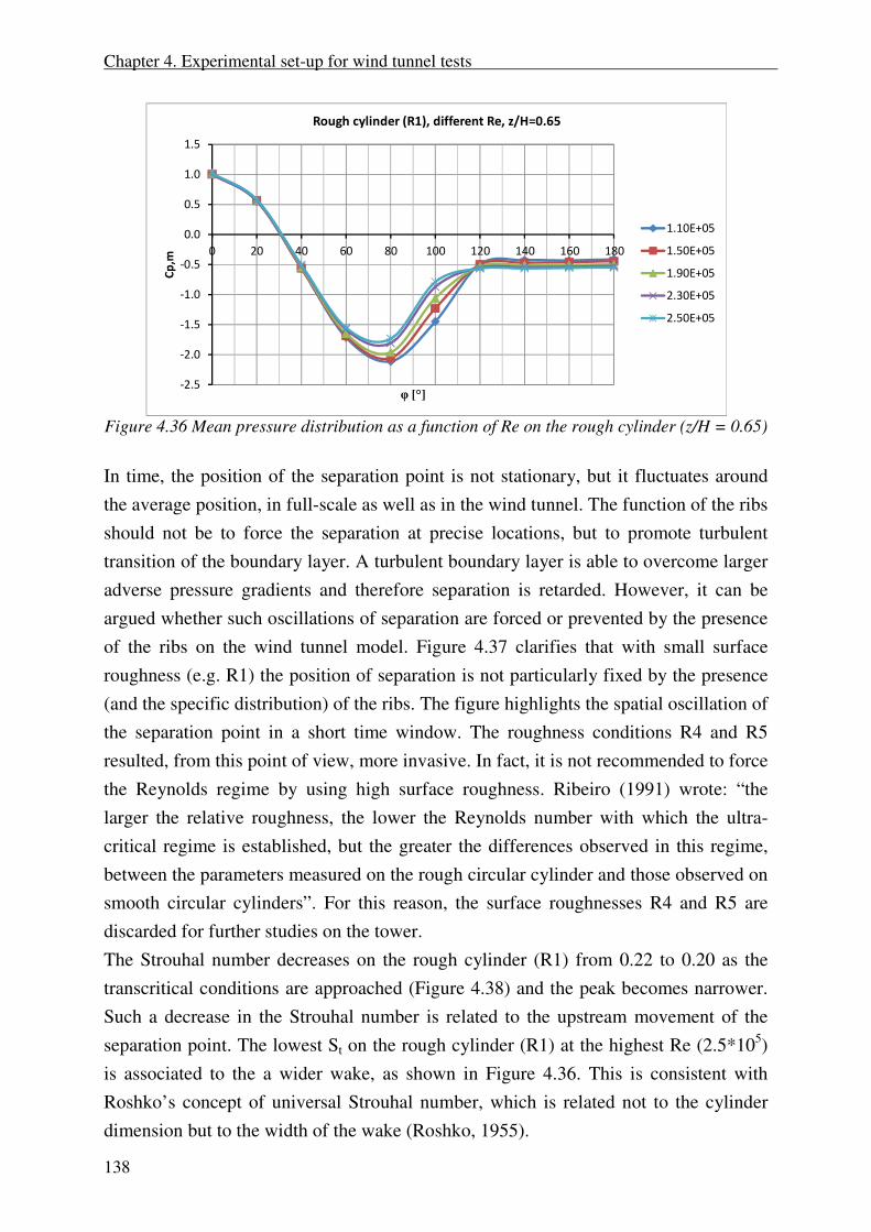
Figure 4.36 Mean pressure distribution as a function of Re on the rough cylinder (z/H = 0.65)

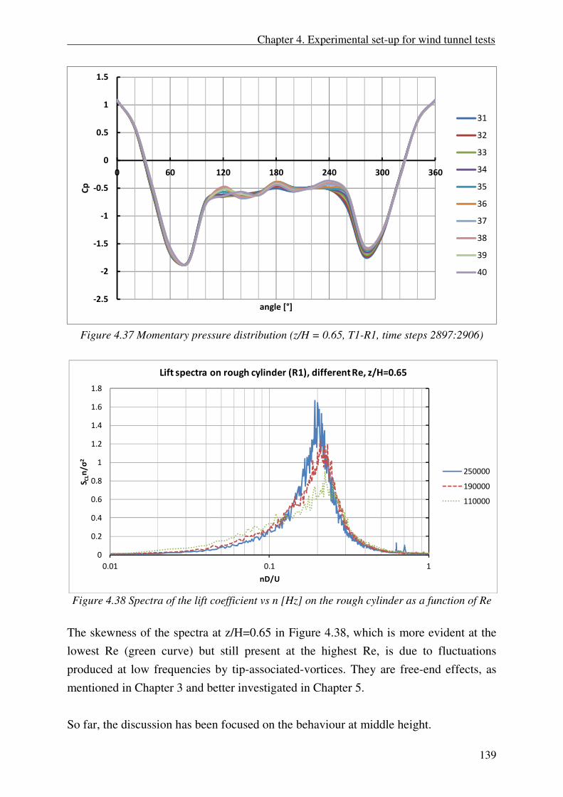
In time, the position of the separation point is not stationary, but it fluctuates around

the average position, in full-scale as well as in the wind tunnel. The function of the ribs

should not be to force the separation at precise locations, but to promote turbulent

transition of the boundary layer. A turbulent boundary layer is able to overcome larger

adverse pressure gradients and therefore separation is retarded. However, it can be

argued whether such oscillations of separation are forced or prevented by the presence

of the ribs on the wind tunnel model. Figure 4.37 clarifies that with small surface

roughness (e.g. R1) the position of separation is not particularly fixed by the presence

(and the specific distribution) of the ribs. The figure highlights the spatial oscillation of

the separation point in a short time window. The roughness conditions R4 and R5

resulted, from this point of view, more invasive. In fact, it is not recommended to force

the Reynolds regime by using high surface roughness. Ribeiro (1991) wrote: “the

larger the relative roughness, the lower the Reynolds number with which the ultra-

critical regime is established, but the greater the differences observed in this regime,

between the parameters measured on the rough circular cylinder and those observed on

smooth circular cylinders”. For this reason, the surface roughnesses R4 and R5 are

discarded for further studies on the tower.

The Strouhal number decreases on the rough cylinder (R1) from 0.22 to 0.20 as the

transcritical conditions are approached (Figure 4.38) and the peak becomes narrower.

Such a decrease in the Strouhal number is related to the upstream movement of the

separation point. The lowest St on the rough cylinder (R1) at the highest Re (2.5*105)

is associated to the a wider wake, as shown in Figure 4.36. This is consistent with

Roshko’s concept of universal Strouhal number, which is related not to the cylinder

dimension but to the width of the wake (Roshko, 1955).

-2.5

-2.0

-1.5

-1.0

-0.5

0.0

0.5

1.0

1.5

0 20 40 60 80 100 120 140 160 180

Cp

,m

φ [°]

Rough cylinder (R1), different Re, z/H=0.65

1.10E+05

1.50E+05

1.90E+05

2.30E+05

2.50E+05


139

Figure 4.37 Momentary pressure distribution (z/H = 0.65, T1-R1, time steps 2897:2906)

Figure 4.38 Spectra of the lift coefficient vs n [Hz] on the rough cylinder as a function of Re

The skewness of the spectra at z/H=0.65 in Figure 4.38, which is more evident at the

lowest Re (green curve) but still present at the highest Re, is due to fluctuations

produced at low frequencies by tip-associated-vortices. They are free-end effects, as

mentioned in Chapter 3 and better investigated in Chapter 5.

So far, the discussion has been focused on the behaviour at middle height.

-2.5

-2

-1.5

-1

-0.5

0

0.5

1

1.5

0 60 120 180 240 300 360

Cp

angle [°]

31

32

33

34

35

36

37

38

39

40

0

0.2

0.4

0.6

0.8

1

1.2

1.4

1.6

1.8

0.01 0.1 1

S CLn

/σ2

nD/U

Lift spectra on rough cylinder (R1), different Re, z/H=0.65

250000

190000

110000


140

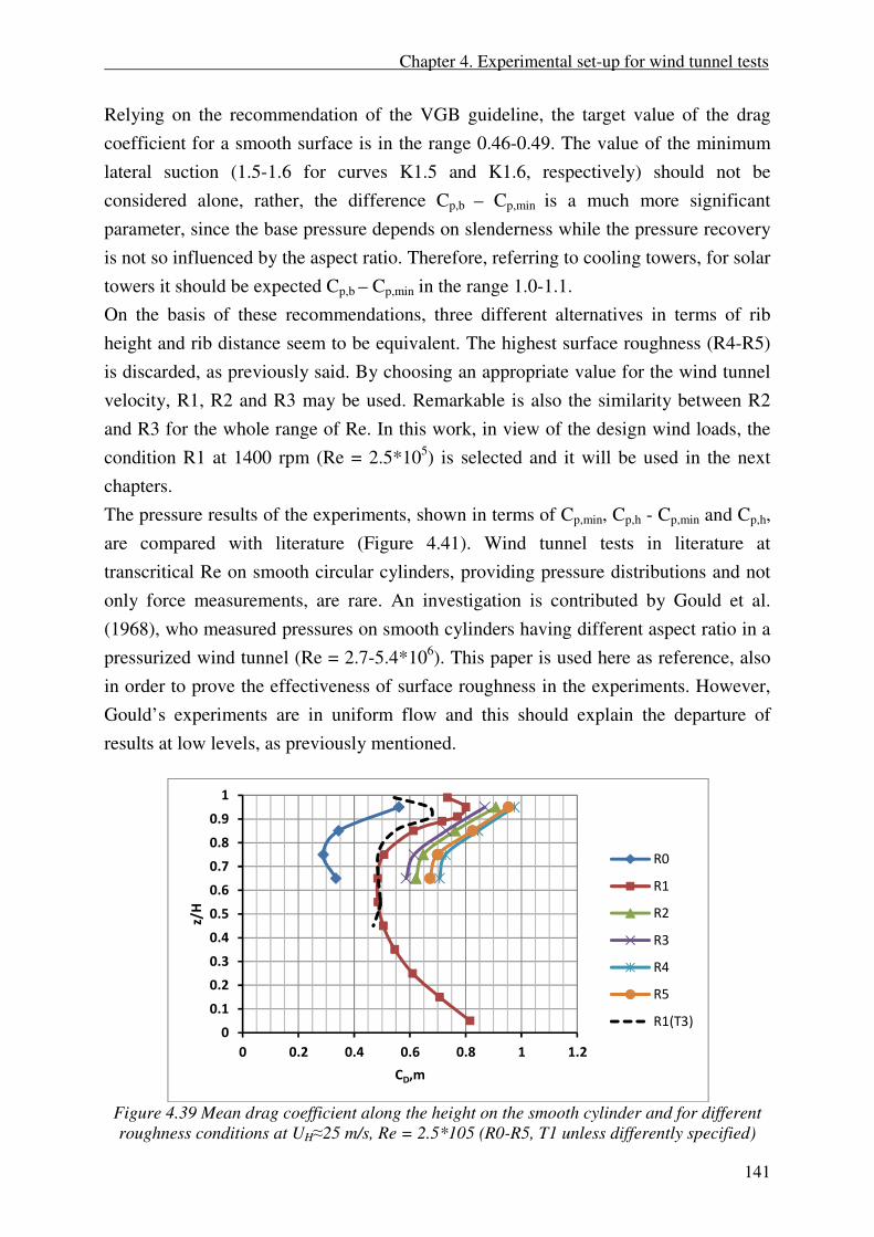
Figure 4.39 and Figure 4.40 describe the spanwise variation of the mean drag

coefficient and of the pressure recovery at Re = 2.5*105. The tip effect is influenced by

the surface roughness, because the rougher is the cylinder, the lower is the wake

pressure (Figure 4.33). This enhances the flow over the tip of the body. For the same

reason, the tip effect on the smooth cylinder is weaker: the smooth cylinder at Re =

2.5*105 is in supercritical conditions, characterized by minimum drag (horizontal

plateau) due to small wake suction and very high pressure recovery due to large

suction at the flanges. Moreover, in uniform flow (black curve) the tip effect is weaker

than in boundary layer flow. It is in contradiction with Gould’s conclusion (Gould et

al., 1968) that the free-end effect is independent on the type of boundary layer. It is

confirmed, instead, that the tip effect produces an increase in the lift fluctuations at

about one diameter from the top, probably due to tip vortices, while the spanwise

variation of drag fluctuations are less pronounced.

Another important feature in Figure 4.39 and Figure 4.40 is the ground effect, which

extends up to z/H = 0.5. It is not only confined to the very low region. The higher drag

at the base of the tower is probably enhanced by the presence of a boundary layer and

thus vertical pressure gradients, as mentioned in Chapter 3. Unfortunately there are not

so many measurements at low levels in uniform flow (T3). In this case, a significant

variation of CD,m would not be expected. In the presence of atmospheric boundary

layer, the ESDU Data Items (ESDU 81017) confirm the existence of higher wake

suction and lower pressure at the flanges. The high wake suction is responsible for an

increase in drag. The even larger lateral suction produces the increase in pressure

recovery as z → 0. In fact, the correction factor proposed by the ESDU Data Items to

account for the atmospheric boundary layer profile (ESDU 81017, figure 5) shows the

same trend as the red curve in Figure 4.39. A similar behaviour of the drag curve at

low levels is confirmed in literature e.g. by Garg’s results (1995) at sub-critical Re, but

a systematic study does not exist. The blue curve in Figure 4.39 (smooth cylinder)

would suggest an even higher three-dimensionality of the phenomenon. However,

there are not measurements in the lower half to confirm it.

The choice of an appropriate surface roughness for the wind tunnel tests, in view of the

evaluation of design wind loads, depends on the full-scale condition which one would

like to achieve. For solar towers, the target full-scale condition is given by a smooth

circular cylinder in transcritical Re. Codified data for smooth and rough surfaces at

transcritical Re are available in the VGB guideline (2010). Further full-scale data on

chimneys and TV towers are collected in (Niemann&Schräder, 1981).


141

Relying on the recommendation of the VGB guideline, the target value of the drag

coefficient for a smooth surface is in the range 0.46-0.49. The value of the minimum

lateral suction (1.5-1.6 for curves K1.5 and K1.6, respectively) should not be

considered alone, rather, the difference Cp,b – Cp,min is a much more significant

parameter, since the base pressure depends on slenderness while the pressure recovery

is not so influenced by the aspect ratio. Therefore, referring to cooling towers, for solar

towers it should be expected Cp,b – Cp,min in the range 1.0-1.1.

On the basis of these recommendations, three different alternatives in terms of rib

height and rib distance seem to be equivalent. The highest surface roughness (R4-R5)

is discarded, as previously said. By choosing an appropriate value for the wind tunnel

velocity, R1, R2 and R3 may be used. Remarkable is also the similarity between R2

and R3 for the whole range of Re. In this work, in view of the design wind loads, the

condition R1 at 1400 rpm (Re = 2.5*105) is selected and it will be used in the next

chapters.

The pressure results of the experiments, shown in terms of Cp,min, Cp,h - Cp,min and Cp,h,

are compared with literature (Figure 4.41). Wind tunnel tests in literature at

transcritical Re on smooth circular cylinders, providing pressure distributions and not

only force measurements, are rare. An investigation is contributed by Gould et al.

(1968), who measured pressures on smooth cylinders having different aspect ratio in a

pressurized wind tunnel (Re = 2.7-5.4*106). This paper is used here as reference, also

in order to prove the effectiveness of surface roughness in the experiments. However,

Gould’s experiments are in uniform flow and this should explain the departure of

results at low levels, as previously mentioned.

Figure 4.39 Mean drag coefficient along the height on the smooth cylinder and for different

roughness conditions at UH≈25 m/s, Re = 2.5*105 (R0-R5, T1 unless differently specified)

0

0.1

0.2

0.3

0.4

0.5

0.6

0.7

0.8

0.9

1

0 0.2 0.4 0.6 0.8 1 1.2

z/H

CD,m

R0

R1

R2

R3

R4

R5

R1(T3)


142

Figure 4.40 Pressure recovery along the height on the smooth cylinder and for different

roughness conditions at UH≈25 m/s, Re = 2.5*105 (R0-R5, T1 unless differently specified)

Figure 4.41 Mean pressure coefficients (Cp,min, Cp,b - Cp,min, Cp,b): red = results by Gould et

al., 1968 (H/D = 6, Re = 5.4*106, uniform flow); blue = WiSt (R1-T1). Green = WiSt (R1-T3,

i.e. uniform flow)

0

0.1

0.2

0.3

0.4

0.5

0.6

0.7

0.8

0.9

1

0 0.2 0.4 0.6 0.8 1 1.2 1.4 1.6 1.8 2

z/H

Cp,b - Cp,min

R0

R1

R2

R3

R4

R5

R1(T3)

0

0.1

0.2

0.3

0.4

0.5

0.6

0.7

0.8

0.9

1

-2.50 -2.00 -1.50 -1.00 -0.50 0.00 0.50 1.00 1.50 2.00

z/H

Cp,m

Cp,b-Cp,min (WiSt)

Cp,b-Cp,min (Gould)

Cp,min (WiSt)

Cp,min (Gould)

Cp,b (WiSt)

Cp,b (Gould)

Uniform flow (WiSt)

Documents

Chapter 4. Experimental set-up for wind tunnel tests