Wind tunnel tests and numerical approach for long span bridges: the Messina bridgeiawe.org/Proceedings/BBAA7/G.Diana.pdf · 2014-03-07 · Wind tunnel tests and numerical approach

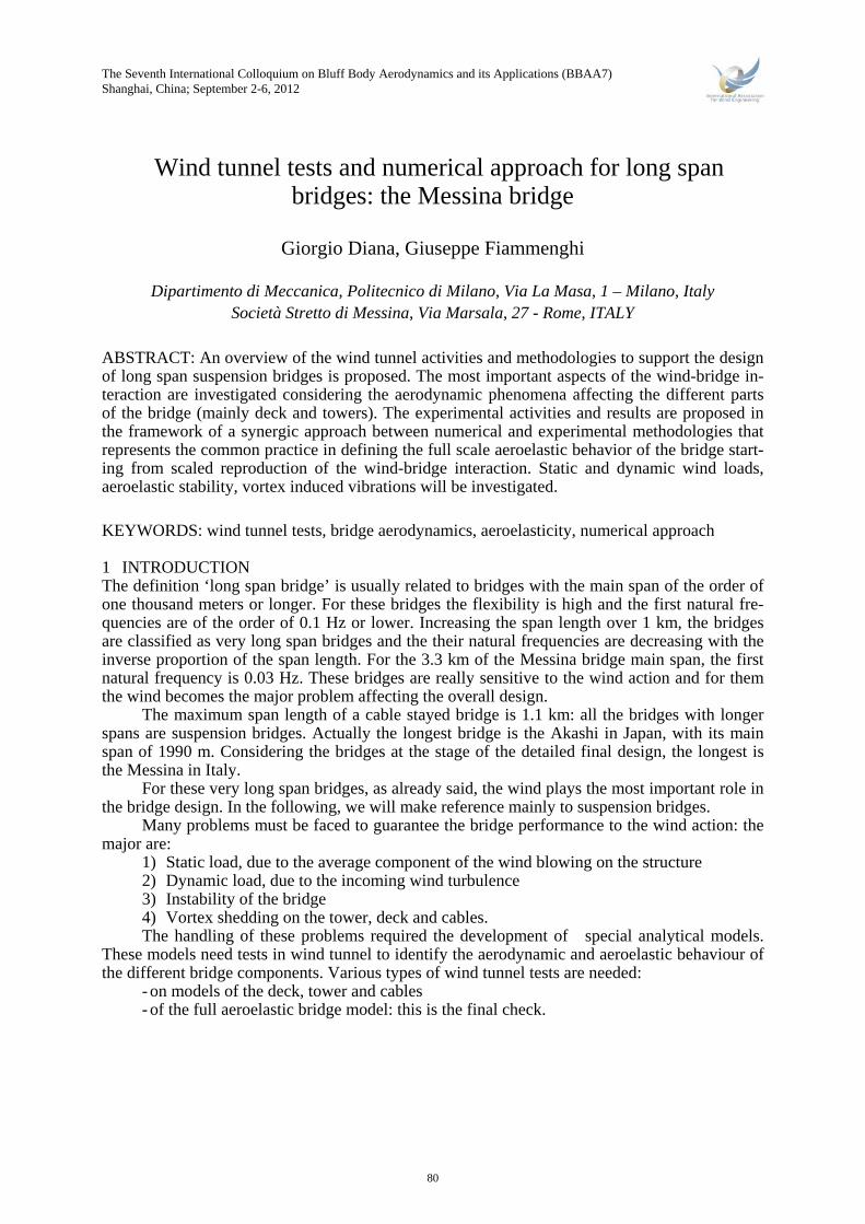
The Seventh International Colloquium on Bluff Body Aerodynamics and its Applications (BBAA7) Shanghai, China; September 2-6, 2012

Wind tunnel tests and numerical approach for long span bridges: the Messina bridge

Giorgio Diana, Giuseppe Fiammenghi

Dipartimento di Meccanica, Politecnico di Milano, Via La Masa, 1 – Milano, Italy Società Stretto di Messina, Via Marsala, 27 - Rome, ITALY

ABSTRACT: An overview of the wind tunnel activities and methodologies to support the design of long span suspension bridges is proposed. The most important aspects of the wind-bridge in-teraction are investigated considering the aerodynamic phenomena affecting the different parts of the bridge (mainly deck and towers). The experimental activities and results are proposed in the framework of a synergic approach between numerical and experimental methodologies that represents the common practice in defining the full scale aeroelastic behavior of the bridge start-ing from scaled reproduction of the wind-bridge interaction. Static and dynamic wind loads, aeroelastic stability, vortex induced vibrations will be investigated.

KEYWORDS: wind tunnel tests, bridge aerodynamics, aeroelasticity, numerical approach 1 INTRODUCTION The definition ‘long span bridge’ is usually related to bridges with the main span of the order of one thousand meters or longer. For these bridges the flexibility is high and the first natural fre-quencies are of the order of 0.1 Hz or lower. Increasing the span length over 1 km, the bridges are classified as very long span bridges and the their natural frequencies are decreasing with the inverse proportion of the span length. For the 3.3 km of the Messina bridge main span, the first natural frequency is 0.03 Hz. These bridges are really sensitive to the wind action and for them the wind becomes the major problem affecting the overall design.

The maximum span length of a cable stayed bridge is 1.1 km: all the bridges with longer spans are suspension bridges. Actually the longest bridge is the Akashi in Japan, with its main span of 1990 m. Considering the bridges at the stage of the detailed final design, the longest is the Messina in Italy.

For these very long span bridges, as already said, the wind plays the most important role in the bridge design. In the following, we will make reference mainly to suspension bridges.

Many problems must be faced to guarantee the bridge performance to the wind action: the major are:

1) Static load, due to the average component of the wind blowing on the structure 2) Dynamic load, due to the incoming wind turbulence 3) Instability of the bridge 4) Vortex shedding on the tower, deck and cables. The handling of these problems required the development of special analytical models.

These models need tests in wind tunnel to identify the aerodynamic and aeroelastic behaviour of the different bridge components. Various types of wind tunnel tests are needed:

- on models of the deck, tower and cables - of the full aeroelastic bridge model: this is the final check.

80

The analytical methods and the experimental tests in the wind tunnel are strongly corre-lated and some of the wind tunnel tests are dedicated to the identification of the aerodynamic and aeroelastic parameters used in the computation programs.

The paper is mainly aimed at describing the numerical tools and the type of wind tunnel tests that are used to design a long span bridge in order to guarantee the correct performances.

It is useful to mention that the Specifications used for the design of the Messina Bridge describe in the detail the type of tests to be carried out in the wind tunnel together with the analy-ses to be performed. These Specifications can be considered as a Standard for long span bridges design.

The present paper is organized in the following paragraphs: 1) Introduction 2) Analytical methods for the analysis of the bridge response to the wind 3) Wind Tunnel tests 4) Numerical results 5) Conclusions.

2 ANALYTICAL METHODS FOR THE ANALYSIS OF THE BRIDGE RESPONSE TO THE

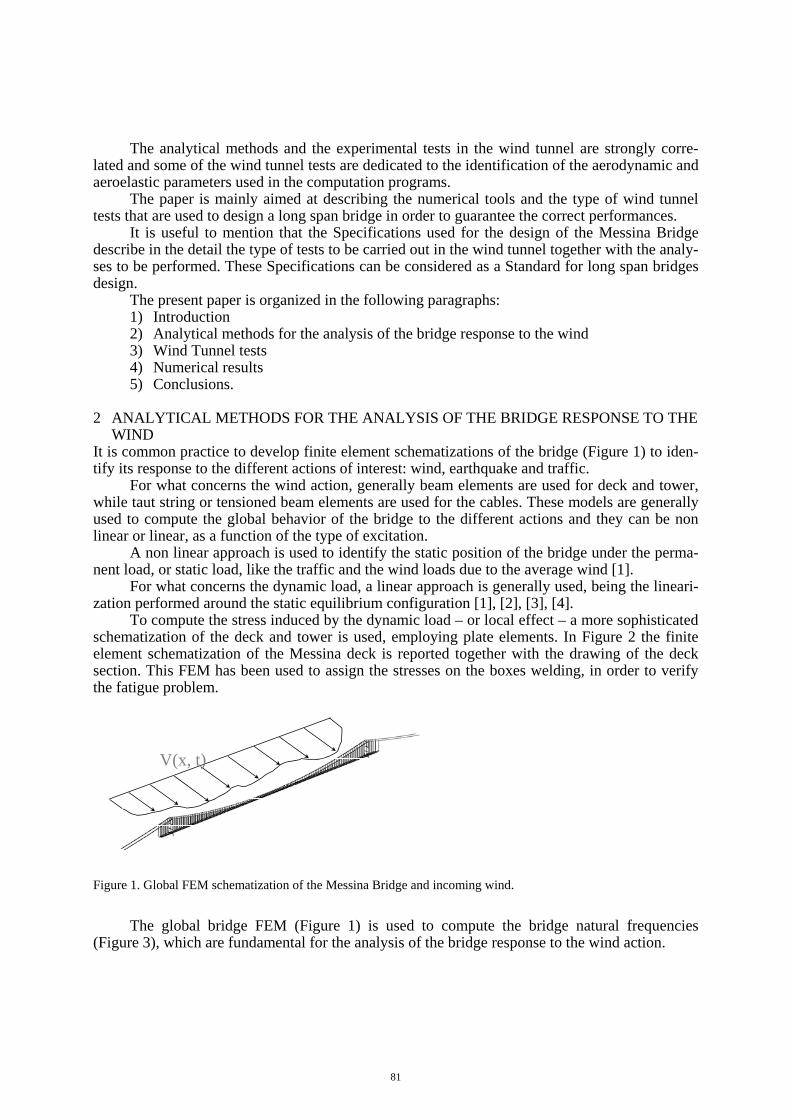
WIND It is common practice to develop finite element schematizations of the bridge (Figure 1) to iden-tify its response to the different actions of interest: wind, earthquake and traffic.

For what concerns the wind action, generally beam elements are used for deck and tower, while taut string or tensioned beam elements are used for the cables. These models are generally used to compute the global behavior of the bridge to the different actions and they can be non linear or linear, as a function of the type of excitation.

A non linear approach is used to identify the static position of the bridge under the perma-nent load, or static load, like the traffic and the wind loads due to the average wind [1].

For what concerns the dynamic load, a linear approach is generally used, being the lineari-zation performed around the static equilibrium configuration [1], [2], [3], [4].

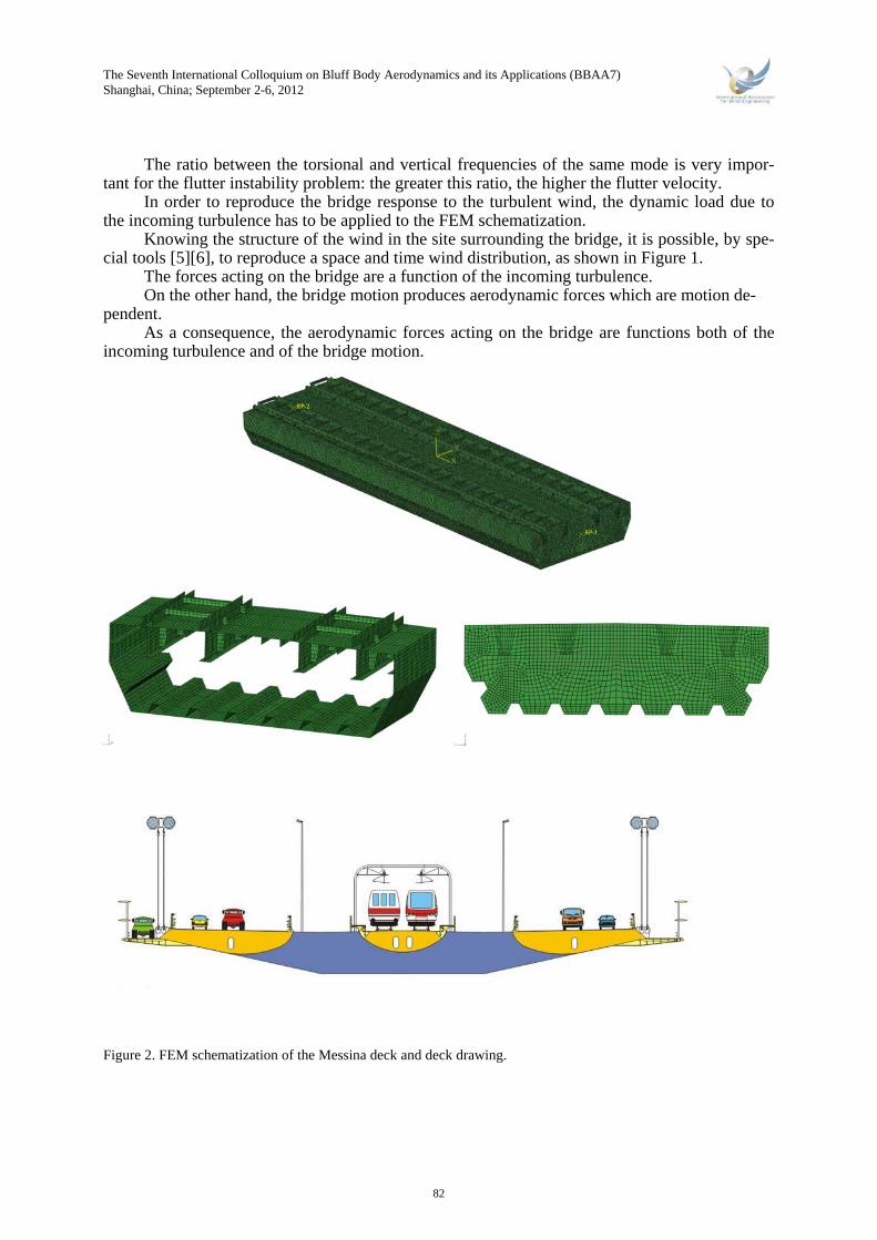
To compute the stress induced by the dynamic load – or local effect – a more sophisticated schematization of the deck and tower is used, employing plate elements. In Figure 2 the finite element schematization of the Messina deck is reported together with the drawing of the deck section. This FEM has been used to assign the stresses on the boxes welding, in order to verify the fatigue problem.

Figure 1. Global FEM schematization of the Messina Bridge and incoming wind.

The global bridge FEM (Figure 1) is used to compute the bridge natural frequencies

(Figure 3), which are fundamental for the analysis of the bridge response to the wind action.

V(x, t)

81


The ratio between the torsional and vertical frequencies of the same mode is very impor-tant for the flutter instability problem: the greater this ratio, the higher the flutter velocity.

In order to reproduce the bridge response to the turbulent wind, the dynamic load due to the incoming turbulence has to be applied to the FEM schematization.

Knowing the structure of the wind in the site surrounding the bridge, it is possible, by spe-cial tools [5][6], to reproduce a space and time wind distribution, as shown in Figure 1.

The forces acting on the bridge are a function of the incoming turbulence. On the other hand, the bridge motion produces aerodynamic forces which are motion de-

pendent. As a consequence, the aerodynamic forces acting on the bridge are functions both of the

incoming turbulence and of the bridge motion.

Figure 2. FEM schematization of the Messina deck and deck drawing.

82

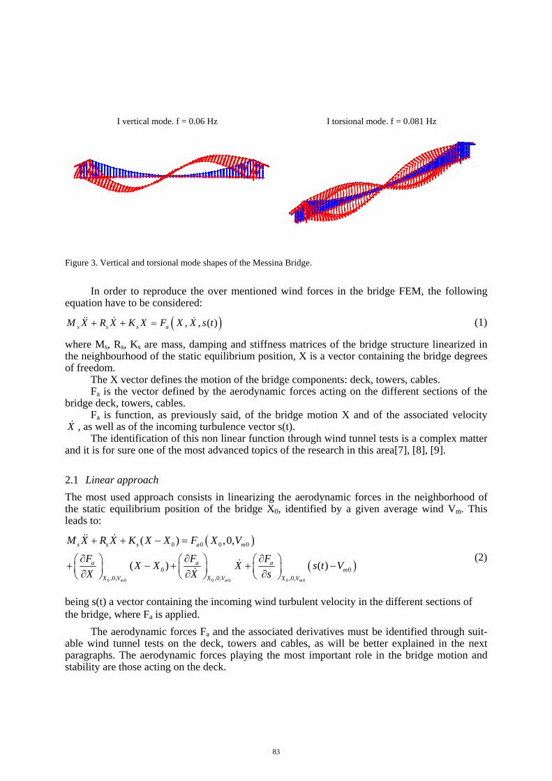
I vertical mode. f = 0.06 Hz I torsional mode. f = 0.081 Hz

Figure 3. Vertical and torsional mode shapes of the Messina Bridge.

In order to reproduce the over mentioned wind forces in the bridge FEM, the following

equation have to be considered:

( ), , ( )s s s aM X R X K X F X X s t+ + =&& & & (1)

where Ms, Rs, Ks are mass, damping and stiffness matrices of the bridge structure linearized in the neighbourhood of the static equilibrium position, X is a vector containing the bridge degrees of freedom.

The X vector defines the motion of the bridge components: deck, towers, cables. Fa is the vector defined by the aerodynamic forces acting on the different sections of the

bridge deck, towers, cables. Fa is function, as previously said, of the bridge motion X and of the associated velocity

X& , as well as of the incoming turbulence vector s(t). The identification of this non linear function through wind tunnel tests is a complex matter

and it is for sure one of the most advanced topics of the research in this area[7], [8], [9].

2.1 Linear approach

The most used approach consists in linearizing the aerodynamic forces in the neighborhood of the static equilibrium position of the bridge X0, identified by a given average wind Vm. This leads to:

( )

( )0 0 0 0 0 0

0 0 0 0

0 0,0, ,0, ,0,

( ) ,0,

( ) ( )m m m

s s s a m

a a am

X V X V X V

M X R X K X X F X V

F F FX X X s t V

X X s

+ + − =

∂ ∂ ∂⎛ ⎞ ⎛ ⎞ ⎛ ⎞+ − + + −⎜ ⎟ ⎜ ⎟ ⎜ ⎟∂ ∂ ∂⎝ ⎠ ⎝ ⎠ ⎝ ⎠

&& &

&&

(2)

being s(t) a vector containing the incoming wind turbulent velocity in the different sections of the bridge, where Fa is applied.

The aerodynamic forces Fa and the associated derivatives must be identified through suit-able wind tunnel tests on the deck, towers and cables, as will be better explained in the next paragraphs. The aerodynamic forces playing the most important role in the bridge motion and stability are those acting on the deck.

83


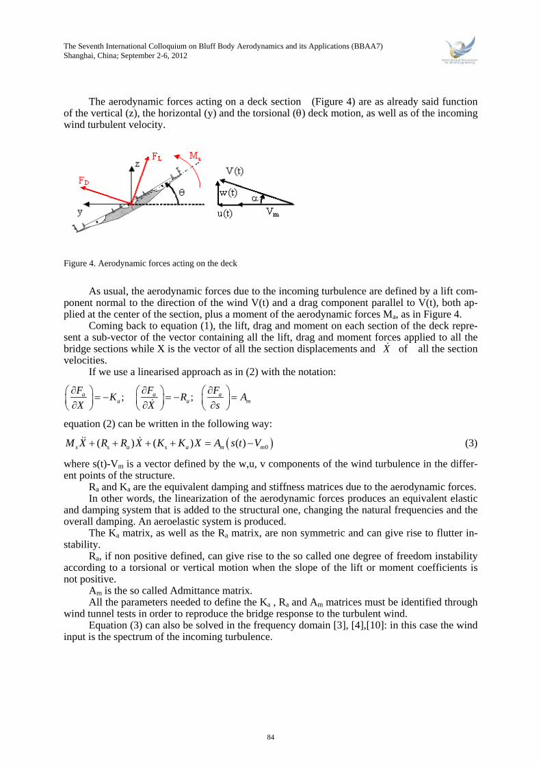
The aerodynamic forces acting on a deck section (Figure 4) are as already said function of the vertical (z), the horizontal (y) and the torsional (θ) deck motion, as well as of the incoming wind turbulent velocity.

Figure 4. Aerodynamic forces acting on the deck

As usual, the aerodynamic forces due to the incoming turbulence are defined by a lift com-

ponent normal to the direction of the wind V(t) and a drag component parallel to V(t), both ap-plied at the center of the section, plus a moment of the aerodynamic forces Ma, as in Figure 4.

Coming back to equation (1), the lift, drag and moment on each section of the deck repre-sent a sub-vector of the vector containing all the lift, drag and moment forces applied to all the bridge sections while X is the vector of all the section displacements and X& of all the section velocities.

If we use a linearised approach as in (2) with the notation:

; ; a a aa a m

F F FK R A

X X s

∂ ∂ ∂⎛ ⎞ ⎛ ⎞ ⎛ ⎞= − = − =⎜ ⎟ ⎜ ⎟ ⎜ ⎟∂ ∂ ∂⎝ ⎠ ⎝ ⎠ ⎝ ⎠&

equation (2) can be written in the following way:

( )0( ) ( ) ( )s s a s a m mM X R R X K K X A s t V+ + + + = −&& & (3)

where s(t)-Vm is a vector defined by the w,u, v components of the wind turbulence in the differ-ent points of the structure.

Ra and Ka are the equivalent damping and stiffness matrices due to the aerodynamic forces. In other words, the linearization of the aerodynamic forces produces an equivalent elastic

and damping system that is added to the structural one, changing the natural frequencies and the overall damping. An aeroelastic system is produced.

The Ka matrix, as well as the Ra matrix, are non symmetric and can give rise to flutter in-stability.

Ra, if non positive defined, can give rise to the so called one degree of freedom instability according to a torsional or vertical motion when the slope of the lift or moment coefficients is not positive.

Am is the so called Admittance matrix. All the parameters needed to define the Ka , Ra and Am matrices must be identified through

wind tunnel tests in order to reproduce the bridge response to the turbulent wind. Equation (3) can also be solved in the frequency domain [3], [4],[10]: in this case the wind

input is the spectrum of the incoming turbulence.

84

2.2 Non Linear approach

Even if linear approaches are the widest adopted method to study the bridge aerodynamic stabil-ity and response of the bridge to turbulent wind they are not able to deal with the important non linear effect intrinsically present in the aeroelastic problem. As already presented, the depend-ence of the aerodynamic forces from the deck motion and from the turbulent wind velocity com-ponents is fully non linear (see equation 2).

( ) ( )( ), , , ,A mM X R X K X F X X V v t w t+ + =&& & &

(4)

The two main causes of non-linearities are the dependence of the aerodynamic forces on

the angle of attack and on the reduced velocity. The QST [10] is able to take into account the de-pendence on the mean angle of attack in a non linear way but it is valid only at high reduced ve-locities. On the contrary the linear approaches are able to take into account the dependence on the reduced velocity through the flutter derivatives and the admittance function coefficients but they represent a solution around a fixed mean angle of attack. Measurements performed on full scale bridges highlighted that during the common operating condition the relative angle of attack between the bridge deck and the wind direction may reach large values that make the linear hy-pothesis not applicable. Some non linear approaches have been developed [7] [8] [9] to deal with the fully non linear aeroelastic problem. In this section we can only introduce the basic ideas of the “Band Superposition” approach and of the “rheological model” approach, and refer the reader to the literature for a more exhaustive description.

The “Band Superposition” approach relies on the possibility of separating the low fre-quency and the high frequency contributions of the wind spectrum. The idea is that the low fre-quency part of the wind spectrum is responsible for the larger fluctuations of the angle of attack and it acts at high reduced velocity. A correct QST [11] is therefore proposed to account for this part taking into account the non linear dependence on the angle of attack. The part of the wind spectrum at high frequency is characterised by smaller amplitudes and lower reduced velocity. To consider the effects induced by this part of the wind spectrum, the aeroelastic forces are lin-earized around the angle of attack that is instantaneously computed by solving the low frequency part of the problem. The problem becomes linear in the high frequency range, but with coeffi-cients changing with the time.

An alternative approach is to consider the whole wind spectrum effects in a single time domain model as represented by the “rheological model”. This approach is based on a numerical model that is able to consider both the angle of attack and the reduced velocity dependence in a single time domain approach. To identify the numerical model parameters, aerodynamic hystere-sis loops are measured on deck sectional models in wind tunnel by changing the instantaneous angle of attack. The variation of the angle if attack is produced by moving the sectional model or by using the active turbulence generator with high amplitudes at different frequencies [7]. 3 WIND TUNNEL TESTS The procedures adopted for the most important long bridges at the design or construction stage will be described. These represent the state of the art on the subject. The tests on deck, towers and cables will be separately considered because the adopted approach is, even if in a small amount, different.

3.1 Aerodynamic tests on the deck

The procedure generally adopted for the wind tunnel tests on the deck is herein after described:

85


1) Static tests on the deck section, in order to measure the lift, drag and moment coeffi-cients as a function of the angle of attack (α). This part is covered in section 3.1.1.

2) Optimization of the deck shape, in order to fulfill the bridge stability requirements, ana-lyzing the slope of the lift and moment coefficients obtained by the static tests (section 3.1.1). This part is described in section 3.1.2.

3) Verification of the vortex shedding excitation, analysing the vibration level as a func-tion of the Scruton number. This will be described in section 3.1.3. If the vibration level fulfils the Specifications at the real bridge Scruton number, the optimization procedure is closed, otherwise the deck shape is changed in order to control vortex shedding and the procedure must be repeated, starting from step 2).

4) Once the deck optimization has been completed, dynamic tests in order to identify the flutter derivatives and the admittance functions should be performed, as reported in de-tail in section 3.1.4.

The optimization procedure from point 1) to 3) is generally performed with small changes of the deck geometry with respect to the preliminary design, such as modification of the wind barriers, if present, or modification of the traffic barriers or parapet screens, or addition of spe-cial devices to control the wind flow.

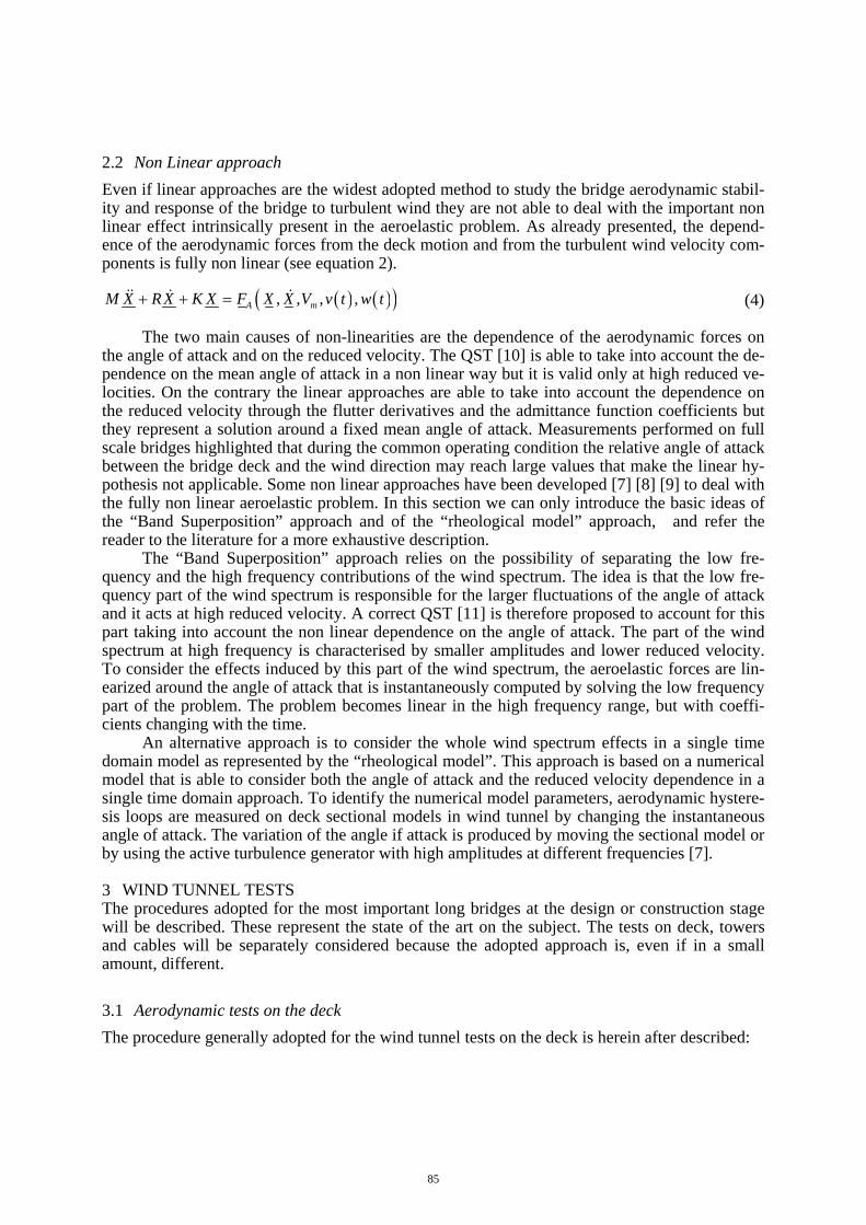
3.1.1 Deck static tests The most important test for the deck, as well as for the other components, is the definition of the static aerodynamic coefficients as a function of the angle of attack.

This test is made in a wind tunnel on a sectional model of the deck (Figure 5) The sectional deck model is placed on a dynamometric system (Figure 5) generally placed

outside the wind tunnel test section [12],[13]. The model can rotate around a deck longitudinal axis and the lift, drag and moment aero-

dynamic forces are measured as a function of the wind angle of attack, by changing the deck an-gle of rotation.

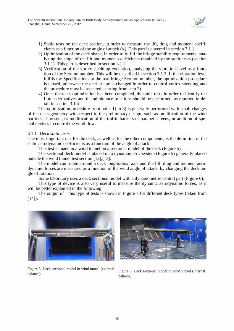
Some laboratory uses a deck sectional model with a dynamometric central part (Figure 6). This type of device is also very useful to measure the dynamic aerodynamic forces, as it

will be better explained in the following. The output of this type of tests is shown in Figure 7 for different deck types (taken from

[14]).

Figure 5. Deck sectional model in wind tunnel (external balance).

Figure 6. Deck sectional model in wind tunnel (internal balance).

86

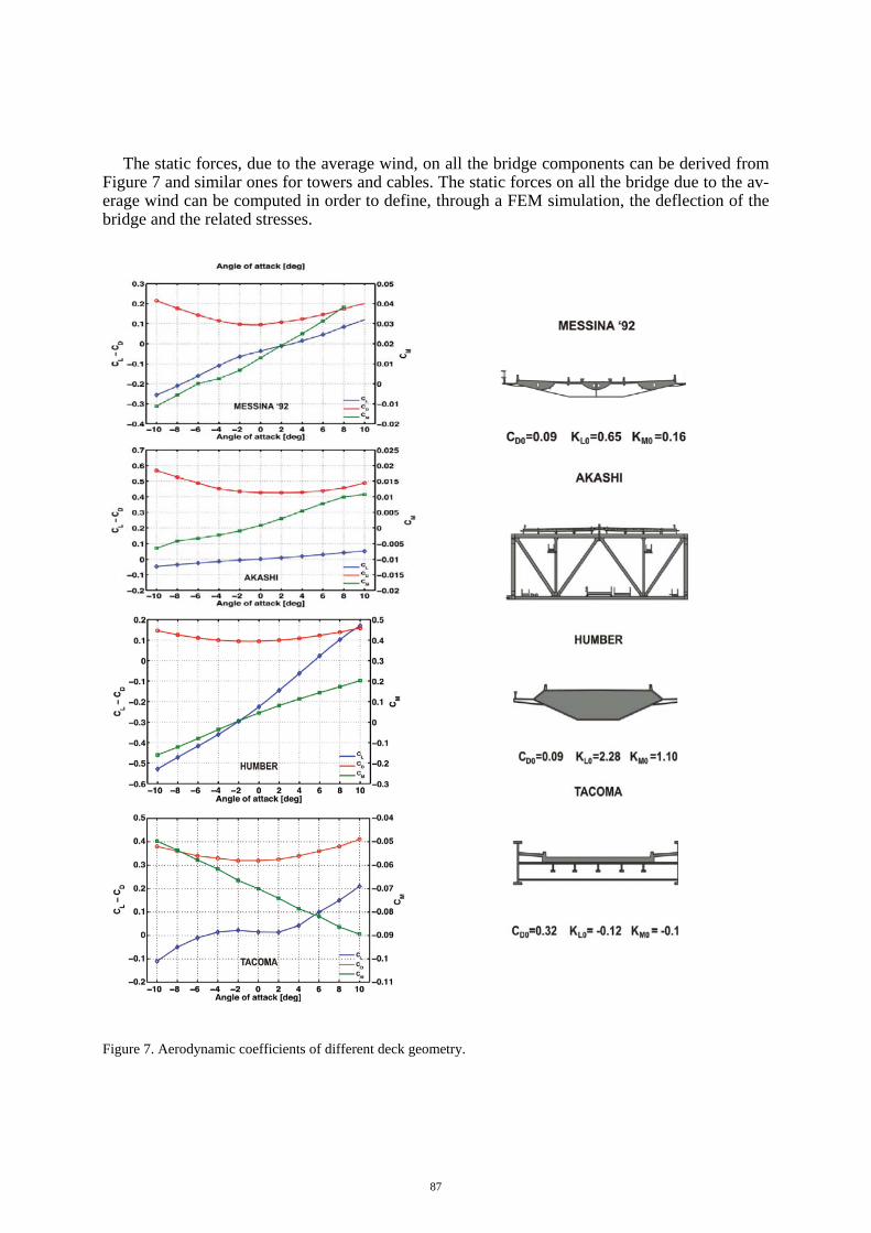
The static forces, due to the average wind, on all the bridge components can be derived from Figure 7 and similar ones for towers and cables. The static forces on all the bridge due to the av-erage wind can be computed in order to define, through a FEM simulation, the deflection of the bridge and the related stresses.

Figure 7. Aerodynamic coefficients of different deck geometry.

87


3.1.2 Aerodynamic optimization of the deck The lift, drag and moment coefficient figures are very important for the bridge deck optimiza-tion.

The moment and lift coefficient slopes are very important for the bridge stability. They must be positive, with the conventions set in Figure 4, to avoid one-degree-of-freedom instability and, in order to have a high flutter velocity, their slopes must be as much as possible lower than the values of a flat plate: 2π for the lift coefficient and π/2 for the moment coefficient.

The slope value to guarantee stability is a function of the ratio between the bridge torsional and vertical frequencies. This ratio is decreasing with the span length: see Figure 8.

In the Messina Specifications the ratio between the first torsional and the first vertical fre-quencies is 1.36, leading to a prescription for a value of the moment coefficient derivative com-prised between 1/5 π/2 and 1/10 π/2 and for a value of the lift coefficient derivative comprised between 1/5 2π and 1/10 2π.

The final reason for this requirement is that the positive slope of the moment coefficient produces a negative torsional stiffness which decreases the torsional frequency, such making it equal to the vertical one and producing the two-degrees-of-freedom flutter instability.

Another important issue is to take the deck drag as low as possible, because the drag forces on the deck are the most important and are transferred to the top of the towers by the hangers and the main cables, producing a moment that affects the overall tower design.

In order to fulfill these requirements, for a very long span bridge – over 2000 m – it is manda-tory to use a multi box section.

A long optimization work is needed to obtain positive lift and moment coefficients with small slopes for all the wind angles of attack, or at least for a ± 4 degrees portion.

For the Messina bridge deck, the optimization involved the railway box shape and the wind barriers shape and porosity both for the road and railway box girders.

Figure 8. Bridge torsional and vertical frequency as a function of the span length

bending (vertical)

torsion

AkashiMessina (railway)Storebaelt

Storebaelt

Kita Bisan-seto(railway)

Minami Bisan-seto(railway)

1000 2000 3000 4000

0.35

0.30

0.25

0.20

0.15

0.10

0.05

0.00

Nat

ura

lF

req

uen

cy

(Hz)

Main Span Length (m)

deck type:

bending (vertical)

torsion

AkashiMessina (railway)Storebaelt

Storebaelt

Kita Bisan-seto(railway)

Minami Bisan-seto(railway)

1000 2000 3000 4000

0.35

0.30

0.25

0.20

0.15

0.10

0.05

0.00

Nat

ura

lF

req

uen

cy

(Hz)

Main Span Length (m)

deck type:

88

3.1.3 Vortex shedding Vortex induced vibrations (VIVs) represent one of the most important aspects of the deck shape design. Even though the bridge deck of the last generation have an airfoil like geometry, flow separation occurs in correspondence of the deck sharp corners, in presence of adverse pressure gradients and of wind shields that are usually adopted to protect traffic. VIV is a serious problem that took also a part in the collapse of the Tacoma Narrow Bridge and has to be carefully ana-lyzed. In fact, even if it can be separated from the stability problem for the modern bridges, it can lead the deck to reach very large vibration amplitudes in case of low Scruton numbers

22 smh

ScB

πρ

= (5)

where m is the mass per unit length, hS is the structural damping, B is the deck chord and ρ is the air density, also at very low wind speeds having a high probability of occurrence.

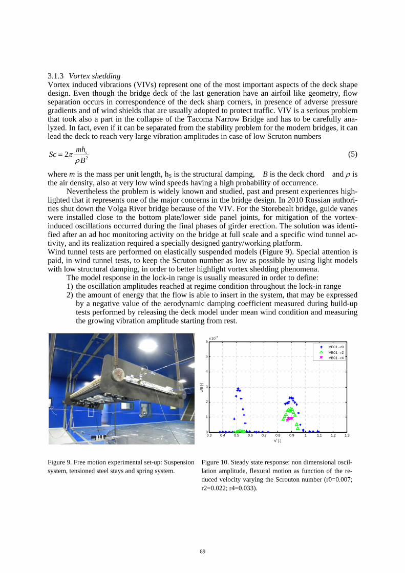
Nevertheless the problem is widely known and studied, past and present experiences high-lighted that it represents one of the major concerns in the bridge design. In 2010 Russian authori-ties shut down the Volga River bridge because of the VIV. For the Storebealt bridge, guide vanes were installed close to the bottom plate/lower side panel joints, for mitigation of the vortex-induced oscillations occurred during the final phases of girder erection. The solution was identi-fied after an ad hoc monitoring activity on the bridge at full scale and a specific wind tunnel ac-tivity, and its realization required a specially designed gantry/working platform. Wind tunnel tests are performed on elastically suspended models (Figure 9). Special attention is paid, in wind tunnel tests, to keep the Scruton number as low as possible by using light models with low structural damping, in order to better highlight vortex shedding phenomena.

The model response in the lock-in range is usually measured in order to define: 1) the oscillation amplitudes reached at regime condition throughout the lock-in range 2) the amount of energy that the flow is able to insert in the system, that may be expressed

by a negative value of the aerodynamic damping coefficient measured during build-up tests performed by releasing the deck model under mean wind condition and measuring the growing vibration amplitude starting from rest.

Figure 9. Free motion experimental set-up: Suspension system, tensioned steel stays and spring system.

Figure 10. Steady state response: non dimensional oscil-lation amplitude, flexural motion as function of the re-duced velocity varying the Scrouton number (r0=0.007; r2=0.022; r4=0.033).

0.3 0.4 0.5 0.6 0.7 0.8 0.9 1 1.1 1.2 1.30

1

2

3

4

5

6x 10

-3

z/B

[-]

V* [-]

MB01 - r0

MB01 - r2

MB01 - r4

89


While single box deck shapes generally shows a single mechanism of vortex shedding, ba-sically related to the vortexes detached in the girder wake, multi box decks may present different vortex shedding phenomena because of the different possibility of flow interactions between the wake of the upwind box and the other boxes.

The different vortex shedding mechanism may excite both the heaving and the torsional motion of the bridge.

As an example Figure 10 presents the two lock-in ranges for the flexural motion of the Messina Bridge multi box deck section for different Scrouton number:

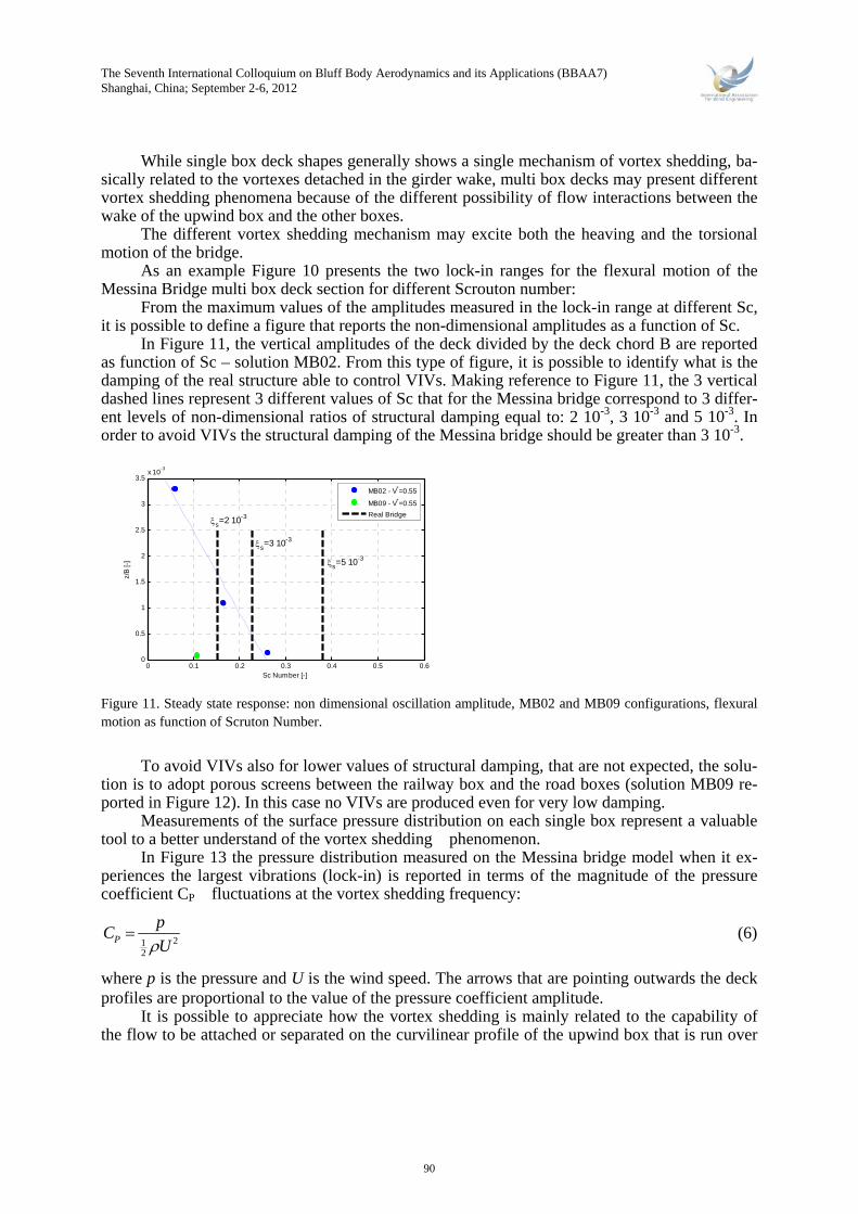
From the maximum values of the amplitudes measured in the lock-in range at different Sc, it is possible to define a figure that reports the non-dimensional amplitudes as a function of Sc.

In Figure 11, the vertical amplitudes of the deck divided by the deck chord B are reported as function of Sc – solution MB02. From this type of figure, it is possible to identify what is the damping of the real structure able to control VIVs. Making reference to Figure 11, the 3 vertical dashed lines represent 3 different values of Sc that for the Messina bridge correspond to 3 differ-ent levels of non-dimensional ratios of structural damping equal to: 2 10-3, 3 10-3 and 5 10-3. In order to avoid VIVs the structural damping of the Messina bridge should be greater than 3 10-3.

0 0.1 0.2 0.3 0.4 0.5 0.60

0.5

1

1.5

2

2.5

3

3.5x 10

-3

Sc Number [-]

z/B

[-]

MB02 - V*=0.55

MB09 - V*=0.55

Real Bridge

ξs=3 10-3

ξs=2 10-3

ξs=5 10-3

Figure 11. Steady state response: non dimensional oscillation amplitude, MB02 and MB09 configurations, flexural motion as function of Scruton Number.

To avoid VIVs also for lower values of structural damping, that are not expected, the solu-

tion is to adopt porous screens between the railway box and the road boxes (solution MB09 re-ported in Figure 12). In this case no VIVs are produced even for very low damping.

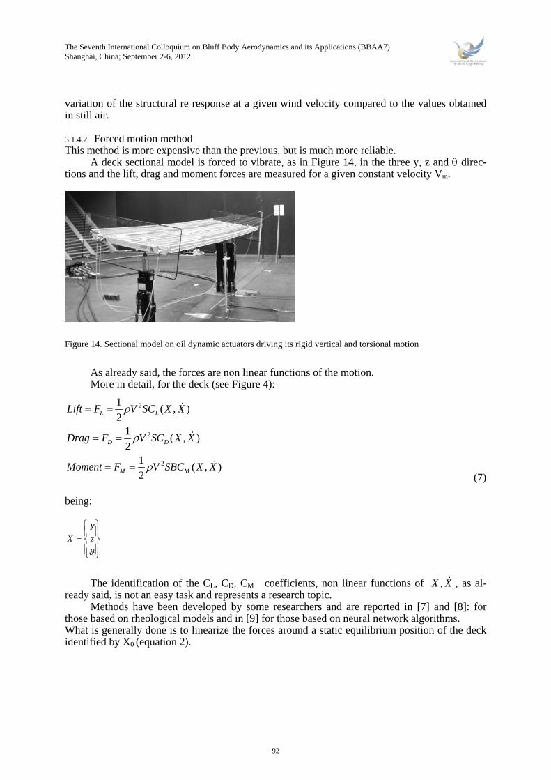
Measurements of the surface pressure distribution on each single box represent a valuable tool to a better understand of the vortex shedding phenomenon.

In Figure 13 the pressure distribution measured on the Messina bridge model when it ex-periences the largest vibrations (lock-in) is reported in terms of the magnitude of the pressure coefficient CP fluctuations at the vortex shedding frequency:

212

P

pC

Uρ= (6)

where p is the pressure and U is the wind speed. The arrows that are pointing outwards the deck profiles are proportional to the value of the pressure coefficient amplitude.

It is possible to appreciate how the vortex shedding is mainly related to the capability of the flow to be attached or separated on the curvilinear profile of the upwind box that is run over

90

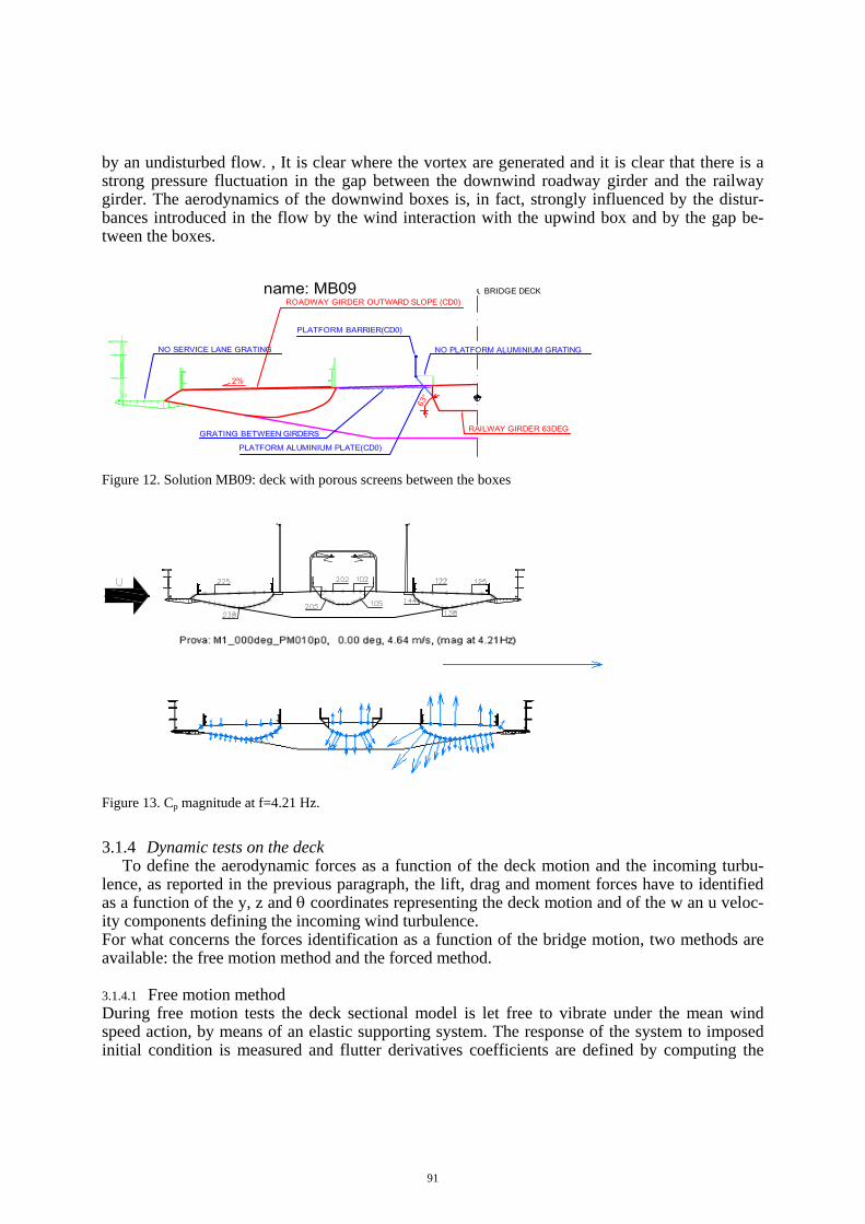
by an undisturbed flow. , It is clear where the vortex are generated and it is clear that there is a strong pressure fluctuation in the gap between the downwind roadway girder and the railway girder. The aerodynamics of the downwind boxes is, in fact, strongly influenced by the distur-bances introduced in the flow by the wind interaction with the upwind box and by the gap be-tween the boxes.

Figure 12. Solution MB09: deck with porous screens between the boxes

Figure 13. Cp magnitude at f=4.21 Hz.

3.1.4 Dynamic tests on the deck To define the aerodynamic forces as a function of the deck motion and the incoming turbu-

lence, as reported in the previous paragraph, the lift, drag and moment forces have to identified as a function of the y, z and θ coordinates representing the deck motion and of the w an u veloc-ity components defining the incoming wind turbulence. For what concerns the forces identification as a function of the bridge motion, two methods are available: the free motion method and the forced method.

3.1.4.1 Free motion method During free motion tests the deck sectional model is let free to vibrate under the mean wind speed action, by means of an elastic supporting system. The response of the system to imposed initial condition is measured and flutter derivatives coefficients are defined by computing the

91


variation of the structural re response at a given wind velocity compared to the values obtained in still air.

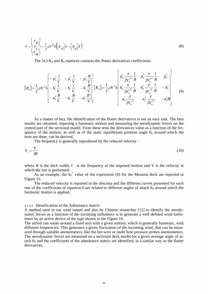
3.1.4.2 Forced motion method This method is more expensive than the previous, but is much more reliable.

A deck sectional model is forced to vibrate, as in Figure 14, in the three y, z and θ direc-tions and the lift, drag and moment forces are measured for a given constant velocity Vm.

Figure 14. Sectional model on oil dynamic actuators driving its rigid vertical and torsional motion

As already said, the forces are non linear functions of the motion. More in detail, for the deck (see Figure 4):

2

2

2

1( , )

21

( , )2

1( , )

2

L L

D D

M M

Lift F V SC X X

Drag F V SC X X

Moment F V SBC X X

ρ

ρ

ρ

= =

= =

= =

&

&

& (7)

being:

⎪⎭

⎪⎬⎫

⎪⎩

⎪⎨⎧

=ϑz

y

X

The identification of the CL, CD, CM coefficients, non linear functions of ,X X& , as al-

ready said, is not an easy task and represents a research topic. Methods have been developed by some researchers and are reported in [7] and [8]: for

those based on rheological models and in [9] for those based on neural network algorithms. What is generally done is to linearize the forces around a static equilibrium position of the deck identified by X0 (equation 2).

92

( )Xa

RXa

KSV

MF

LFD

F

F &⎥⎦⎤

⎢⎣⎡+⎥⎦

⎤⎢⎣⎡==

⎪⎭

⎪⎬

⎫

⎪⎩

⎪⎨

⎧2

2

1ρ (8)

The 3x3 Ka and Ra matrices contains the flutter derivatives coefficients:

[ ]

⎥⎥⎥⎥⎥⎥

⎦

⎤

⎢⎢⎢⎢⎢⎢

⎣

⎡

−−−

−−−

−−−

=

V

Ba

V

Ba

V

Ba

V

Bh

Vh

Vh

V

Bp

Vp

Vp

SVRa

2*2

*1

*5

*2

*1

*5

*2

*1

*5

2 11

11

2

1 ρ [ ]

⎥⎥⎥⎥⎥⎥⎥

⎦

⎤

⎢⎢⎢⎢⎢⎢⎢

⎣

⎡

−

−=

BaV

aV

a

hBV

hBV

h

pBV

pBV

p

SVKa

*32*

*42*

*6

*32*

*42*

*6

*32*

*42*

*6

2

22

1

2

1

2

1

2

1

2

2

1

ωω

ωω

ωω

ππ

ππ

ππ

ρ (9)

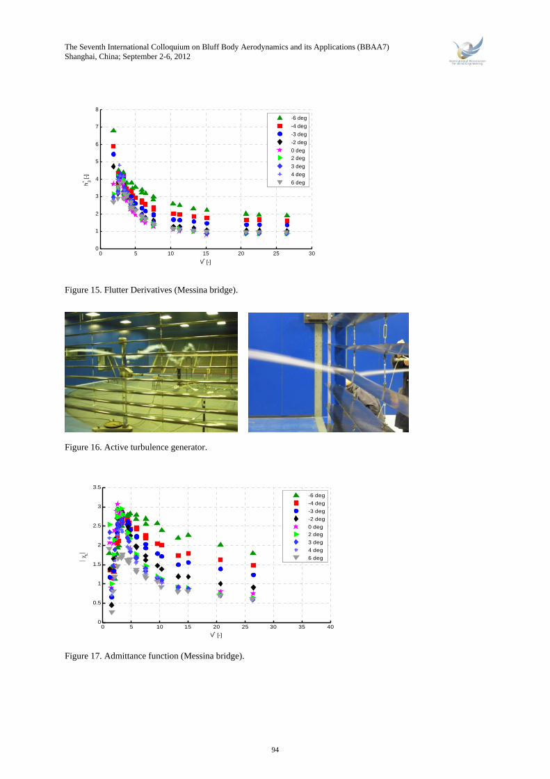
As a matter of fact, the identification of the flutter derivatives is not an easy task. The best results are obtained, imposing a harmonic motion and measuring the aerodynamic forces on the central part of the sectional model. From these tests the derivatives value as a function of the fre-quency of the motion, as well as of the static equilibrium position angle θ0 around which the tests are done, can be derived.

The frequency is generally reproduced by the reduced velocity

r

VV

fB= (10)

where B is the deck width, f is the frequency of the imposed motion and V is the velocity at which the test is performed.

As an example, the h3* value of the expression (9) for the Messina deck are reported in

Figure 15. The reduced velocity is reported in the abscissa and the different curves presented for each

one of the coefficients of equation 6 are related to different angles of attack θ0 around which the harmonic motion is applied.

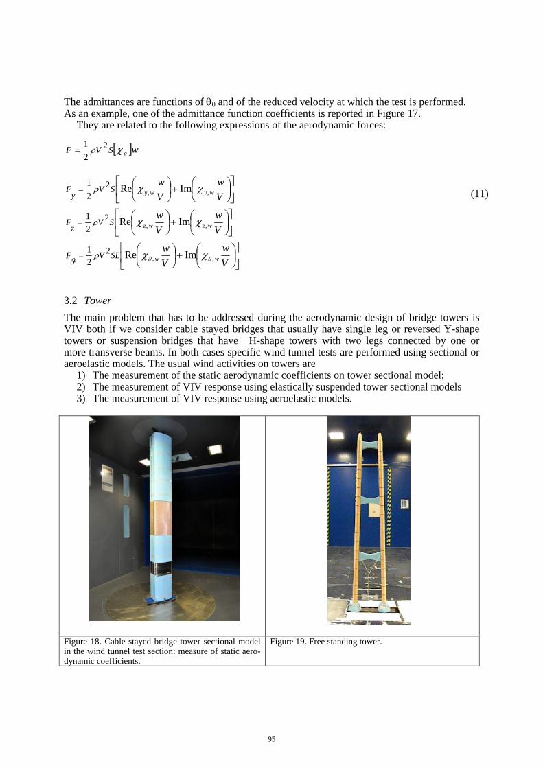
3.1.4.3 Identification of the Admittance matrix A method used in our wind tunnel and also by Chinese researcher [12] to identify the aerody-namic forces as a function of the incoming turbulence is to generate a well defined wind turbu-lence by an active device of the type shown in the Figure 16. The airfoil can rotate around a fixed axis with a given motion, which is generally harmonic, with different frequencies. This generates a given fluctuation of the incoming wind, that can be meas-ured through suitable anemometers, like the hot-wire or multi hole pressure probes anemometers. The aerodynamic forces are measured on a sectional deck model for a given average angle of at-tack θ0 and the coefficients of the admittance matrix are identified, in a similar way as the flutter derivatives.

93


0 5 10 15 20 25 300

1

2

3

4

5

6

7

8

V* [-]

h* 3 [-

]

-6 deg

-4 deg

-3 deg

-2 deg

0 deg

2 deg

3 deg

4 deg

6 deg

Figure 15. Flutter Derivatives (Messina bridge).

Figure 16. Active turbulence generator.

0 5 10 15 20 25 30 35 400

0.5

1

1.5

2

2.5

3

3.5

V* [-]

⏐χL⏐

-6 deg

-4 deg

-3 deg

-2 deg

0 deg

2 deg

3 deg

4 deg

6 deg

Figure 17. Admittance function (Messina bridge).

94

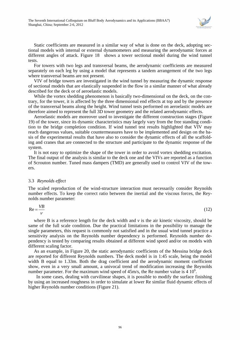
(11)

The admittances are functions of θ0 and of the reduced velocity at which the test is performed. As an example, one of the admittance function coefficients is reported in Figure 17.

They are related to the following expressions of the aerodynamic forces:

[ ]waSVF χρ 22

1=

⎥⎦

⎤⎢⎣

⎡⎟⎠⎞

⎜⎝⎛+⎟

⎠⎞

⎜⎝⎛

⎥⎦

⎤⎢⎣

⎡⎟⎠⎞

⎜⎝⎛+⎟

⎠⎞

⎜⎝⎛

⎥⎦

⎤⎢⎣

⎡⎟⎠⎞

⎜⎝⎛+⎟

⎠⎞

⎜⎝⎛

=

=

=

V

w

V

w

V

w

V

w

V

w

V

w

ww

wzwz

wywy

SLVF

SVz

F

SVy

F

,,

,,

,,

ImRe

ImRe

ImRe

22

1

22

1

22

1

ϑϑ χχ

χχ

χχ

ρϑ

ρ

ρ

3.2 Tower

The main problem that has to be addressed during the aerodynamic design of bridge towers is VIV both if we consider cable stayed bridges that usually have single leg or reversed Y-shape towers or suspension bridges that have H-shape towers with two legs connected by one or more transverse beams. In both cases specific wind tunnel tests are performed using sectional or aeroelastic models. The usual wind activities on towers are

1) The measurement of the static aerodynamic coefficients on tower sectional model; 2) The measurement of VIV response using elastically suspended tower sectional models 3) The measurement of VIV response using aeroelastic models.

Figure 18. Cable stayed bridge tower sectional model in the wind tunnel test section: measure of static aero-dynamic coefficients.

Figure 19. Free standing tower.

95


Static coefficients are measured in a similar way of what is done on the deck, adopting sec-tional models with internal or external dynamometers and measuring the aerodynamic forces at different angles of attack. Figure 18 shows a tower sectional model during the wind tunnel tests.

For towers with two legs and transversal beams, the aerodynamic coefficients are measured separately on each leg by using a model that represents a tandem arrangement of the two legs where transversal beams are not present.

VIV of bridge towers are investigated in the wind tunnel by measuring the dynamic response of sectional models that are elastically suspended in the flow in a similar manner of what already described for the deck or of aeroelastic models.

While the vortex shedding phenomenon is basically two-dimensional on the deck, on the con-trary, for the tower, it is affected by the three dimensional end effects at top and by the presence of the transversal beams along the height. Wind tunnel tests performed on aeroelastic models are therefore aimed to represent the full 3D tower geometry and the related aerodynamic effects.

Aeroelastic models are moreover used to investigate the different construction stages (Figure 19) of the tower, since its dynamic characteristics may largely vary from the free standing condi-tion to the bridge completion condition. If wind tunnel test results highlighted that VIV may reach dangerous values, suitable countermeasures have to be implemented and design on the ba-sis of the experimental results that have also to consider the dynamic effects of all the scaffold-ing and cranes that are connected to the structure and participate to the dynamic response of the system.

It is not easy to optimize the shape of the tower in order to avoid vortex shedding excitation. The final output of the analysis is similar to the deck one and the VIVs are reported as a function of Scrouton number. Tuned mass dampers (TMD) are generally used to control VIV of the tow-ers.

3.3 Reynolds effect

The scaled reproduction of the wind-structure interaction must necessarily consider Reynolds number effects. To keep the correct ratio between the inertial and the viscous forces, the Rey-nolds number parameter:

ReVB

ν= (12)

where B is a reference length for the deck width and v is the air kinetic viscosity, should be same of the full scale condition. Due the practical limitations in the possibility to manage the single parameters, this request is commonly not satisfied and in the usual wind tunnel practice a sensitivity analysis on the Reynolds number dependency is performed. Reynolds number de-pendency is tested by comparing results obtained at different wind speed and/or on models with different scaling factor.

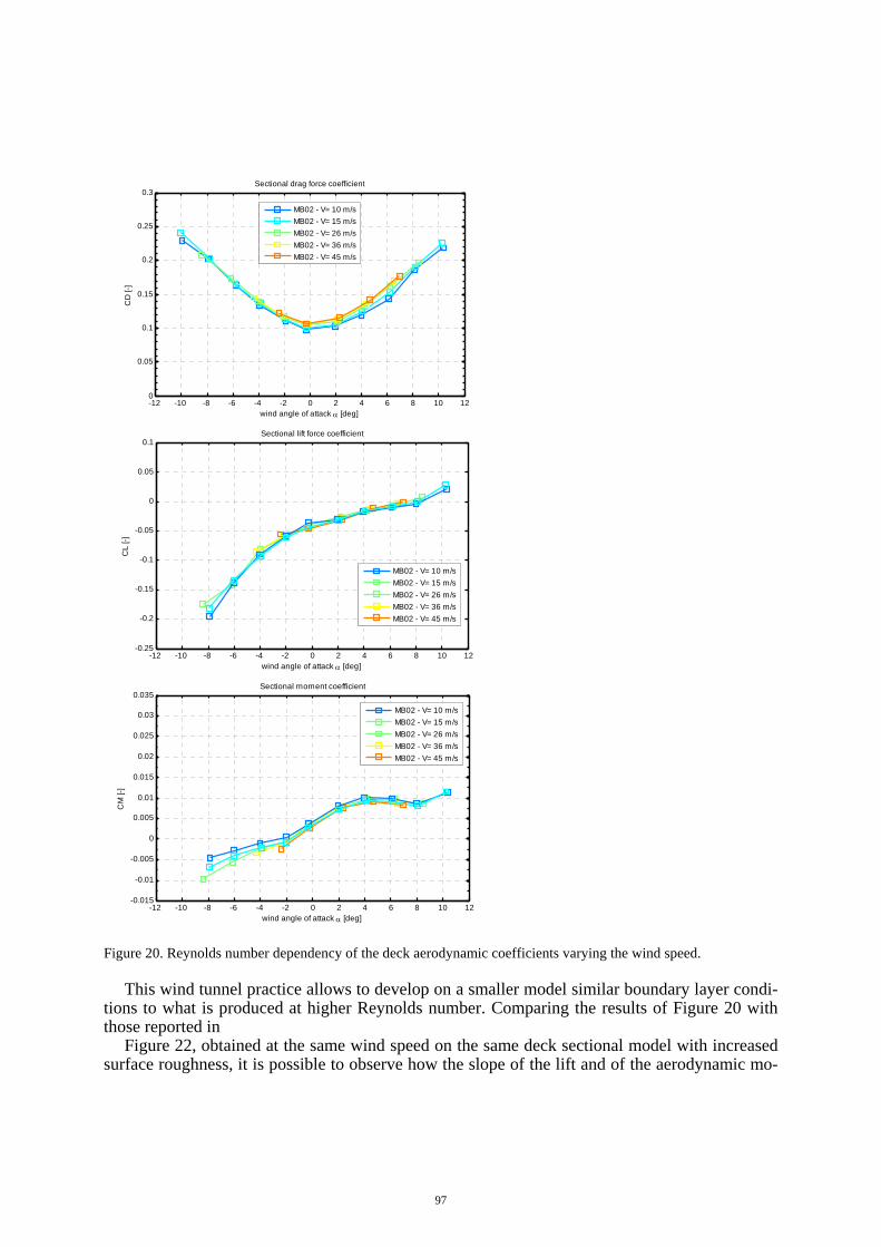
As an example, in Figure 20, the static aerodynamic coefficients of the Messina bridge deck are reported for different Reynolds numbers. The deck model is in 1:45 scale, being the model width B equal to 1.33m. Both the drag coefficient and the aerodynamic moment coefficient show, even in a very small amount, a univocal trend of modification increasing the Reynolds number parameter. For the maximum wind speed of 45m/s, the Re number value is 4 106.

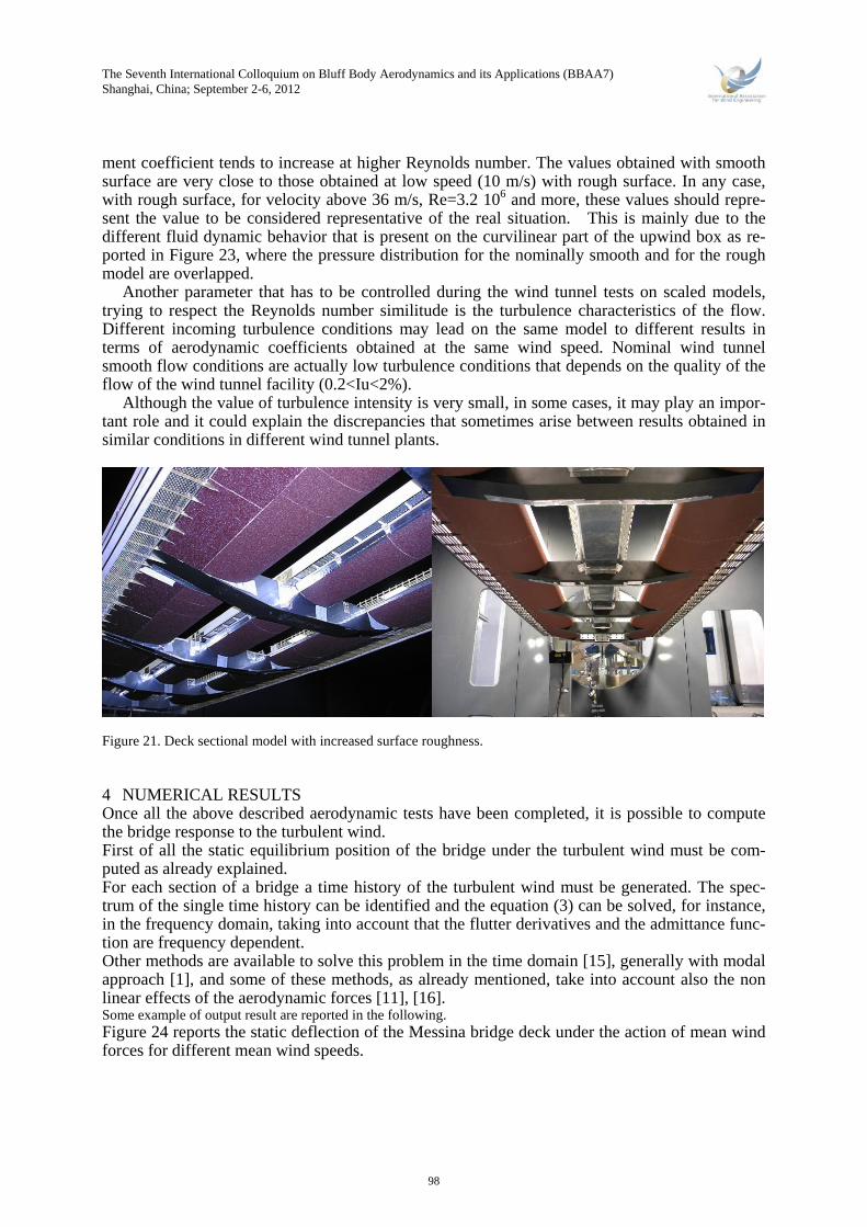
In some cases, dealing with curvilinear shapes, it is possible to modify the surface finishing by using an increased roughness in order to simulate at lower Re similar fluid dynamic effects of higher Reynolds number conditions (Figure 21).

96

-12 -10 -8 -6 -4 -2 0 2 4 6 8 10 120

0.05

0.1

0.15

0.2

0.25

0.3

wind angle of attack α [deg]

CD

[-]

Sectional drag force coefficient

MB02 - V= 10 m/s

MB02 - V= 15 m/s

MB02 - V= 26 m/s

MB02 - V= 36 m/s

MB02 - V= 45 m/s

-12 -10 -8 -6 -4 -2 0 2 4 6 8 10 12-0.25

-0.2

-0.15

-0.1

-0.05

0

0.05

0.1


CL

[-]

Sectional lift force coefficient

MB02 - V= 10 m/s

MB02 - V= 15 m/s

MB02 - V= 26 m/s

MB02 - V= 36 m/s

MB02 - V= 45 m/s

-12 -10 -8 -6 -4 -2 0 2 4 6 8 10 12-0.015

-0.01

-0.005

0

0.005

0.01

0.015

0.02

0.025

0.03

0.035


CM

[-]

Sectional moment coefficient

MB02 - V= 10 m/s

MB02 - V= 15 m/s

MB02 - V= 26 m/s

MB02 - V= 36 m/s

MB02 - V= 45 m/s

Figure 20. Reynolds number dependency of the deck aerodynamic coefficients varying the wind speed.

This wind tunnel practice allows to develop on a smaller model similar boundary layer condi-

tions to what is produced at higher Reynolds number. Comparing the results of Figure 20 with those reported in

Figure 22, obtained at the same wind speed on the same deck sectional model with increased surface roughness, it is possible to observe how the slope of the lift and of the aerodynamic mo-

97


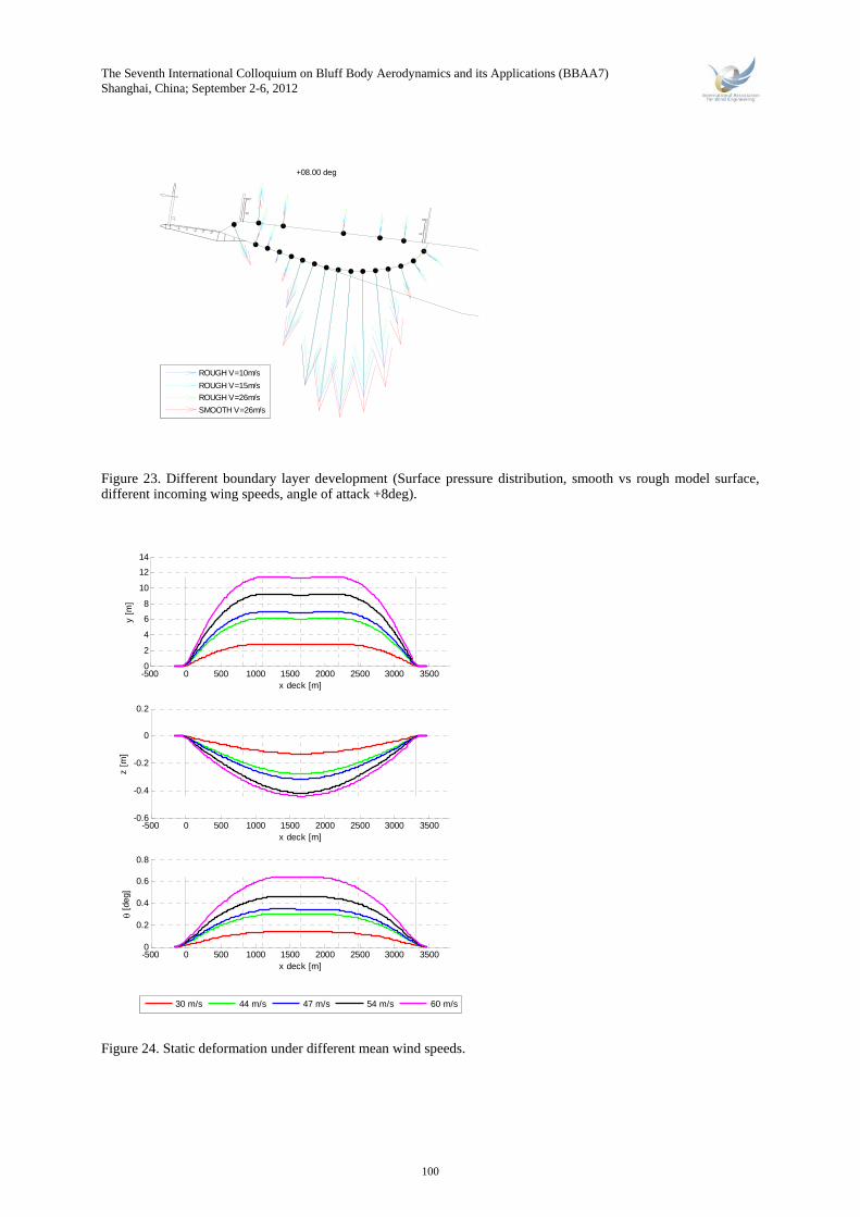
ment coefficient tends to increase at higher Reynolds number. The values obtained with smooth surface are very close to those obtained at low speed (10 m/s) with rough surface. In any case, with rough surface, for velocity above 36 m/s, Re=3.2 106 and more, these values should repre-sent the value to be considered representative of the real situation. This is mainly due to the different fluid dynamic behavior that is present on the curvilinear part of the upwind box as re-ported in Figure 23, where the pressure distribution for the nominally smooth and for the rough model are overlapped.

Another parameter that has to be controlled during the wind tunnel tests on scaled models, trying to respect the Reynolds number similitude is the turbulence characteristics of the flow. Different incoming turbulence conditions may lead on the same model to different results in terms of aerodynamic coefficients obtained at the same wind speed. Nominal wind tunnel smooth flow conditions are actually low turbulence conditions that depends on the quality of the flow of the wind tunnel facility (0.2<Iu<2%).

Although the value of turbulence intensity is very small, in some cases, it may play an impor-tant role and it could explain the discrepancies that sometimes arise between results obtained in similar conditions in different wind tunnel plants.

Figure 21. Deck sectional model with increased surface roughness.

4 NUMERICAL RESULTS Once all the above described aerodynamic tests have been completed, it is possible to compute the bridge response to the turbulent wind. First of all the static equilibrium position of the bridge under the turbulent wind must be com-puted as already explained. For each section of a bridge a time history of the turbulent wind must be generated. The spec-trum of the single time history can be identified and the equation (3) can be solved, for instance, in the frequency domain, taking into account that the flutter derivatives and the admittance func-tion are frequency dependent. Other methods are available to solve this problem in the time domain [15], generally with modal approach [1], and some of these methods, as already mentioned, take into account also the non linear effects of the aerodynamic forces [11], [16]. Some example of output result are reported in the following. Figure 24 reports the static deflection of the Messina bridge deck under the action of mean wind forces for different mean wind speeds.

98

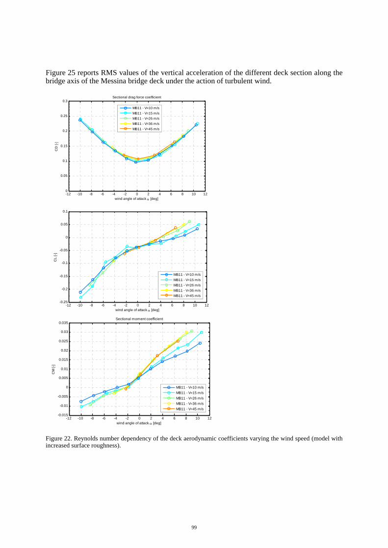
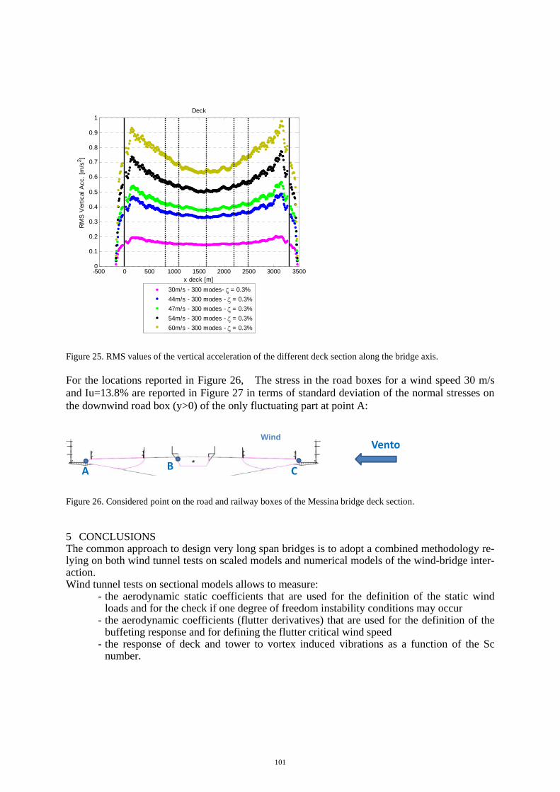
Figure 25 reports RMS values of the vertical acceleration of the different deck section along the bridge axis of the Messina bridge deck under the action of turbulent wind.

-12 -10 -8 -6 -4 -2 0 2 4 6 8 10 120

0.05

0.1

0.15

0.2

0.25

0.3


CD

[-]

Sectional drag force coefficient

MB11 - V=10 m/s

MB11 - V=15 m/s

MB11 - V=26 m/s

MB11 - V=36 m/s

MB11 - V=45 m/s

-12 -10 -8 -6 -4 -2 0 2 4 6 8 10 12-0.25

-0.2

-0.15

-0.1

-0.05

0

0.05

0.1


CL

[-]

MB11 - V=10 m/s

MB11 - V=15 m/s

MB11 - V=26 m/s

MB11 - V=36 m/s

MB11 - V=45 m/s

-12 -10 -8 -6 -4 -2 0 2 4 6 8 10 12-0.015

-0.01

-0.005

0

0.005

0.01

0.015

0.02

0.025

0.03

0.035


CM

[-]

Sectional moment coefficient

MB11 - V=10 m/s

MB11 - V=15 m/s

MB11 - V=26 m/s

MB11 - V=36 m/s

MB11 - V=45 m/s

Figure 22. Reynolds number dependency of the deck aerodynamic coefficients varying the wind speed (model with increased surface roughness).

99


+08.00 deg

ROUGH V=10m/s

ROUGH V=15m/s

ROUGH V=26m/s

SMOOTH V=26m/s

Figure 23. Different boundary layer development (Surface pressure distribution, smooth vs rough model surface, different incoming wing speeds, angle of attack +8deg).

-500 0 500 1000 1500 2000 2500 3000 35000

2

4

6

8

10

12

14

x deck [m]

y [m

]

-500 0 500 1000 1500 2000 2500 3000 3500-0.6

-0.4

-0.2

0

0.2

x deck [m]

z [m

]

-500 0 500 1000 1500 2000 2500 3000 35000

0.2

0.4

0.6

0.8

x deck [m]

θ [d

eg]

30 m/s 44 m/s 47 m/s 54 m/s 60 m/s

Figure 24. Static deformation under different mean wind speeds.

100

-500 0 500 1000 1500 2000 2500 3000 35000

0.1

0.2

0.3

0.4

0.5

0.6

0.7

0.8

0.9

1

RM

S V

ertic

al A

cc.

[m/s

2 ]

x deck [m]

Deck

30m/s - 300 modes- ζ = 0.3%

44m/s - 300 modes - ζ = 0.3%

47m/s - 300 modes - ζ = 0.3%

54m/s - 300 modes - ζ = 0.3%

60m/s - 300 modes - ζ = 0.3%

Figure 25. RMS values of the vertical acceleration of the different deck section along the bridge axis.

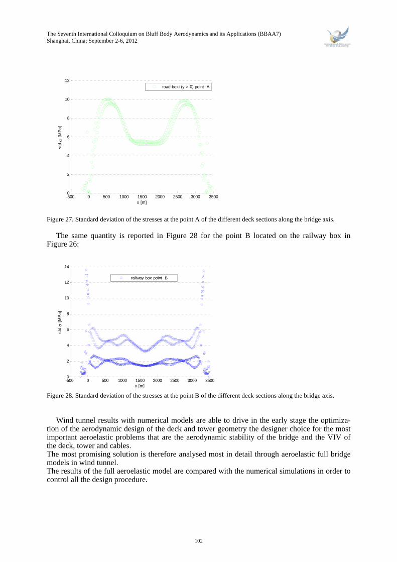
For the locations reported in Figure 26, The stress in the road boxes for a wind speed 30 m/s and Iu=13.8% are reported in Figure 27 in terms of standard deviation of the normal stresses on the downwind road box (y>0) of the only fluctuating part at point A:

A B

Vento

C

Figure 26. Considered point on the road and railway boxes of the Messina bridge deck section.

5 CONCLUSIONS The common approach to design very long span bridges is to adopt a combined methodology re-lying on both wind tunnel tests on scaled models and numerical models of the wind-bridge inter-action. Wind tunnel tests on sectional models allows to measure:

- the aerodynamic static coefficients that are used for the definition of the static wind loads and for the check if one degree of freedom instability conditions may occur

- the aerodynamic coefficients (flutter derivatives) that are used for the definition of the buffeting response and for defining the flutter critical wind speed

- the response of deck and tower to vortex induced vibrations as a function of the Sc number.

Wind

101


-500 0 500 1000 1500 2000 2500 3000 35000

2

4

6

8

10

12

x [m]

std

σ [

MP

a]

road boxi (y > 0) point A

Figure 27. Standard deviation of the stresses at the point A of the different deck sections along the bridge axis.

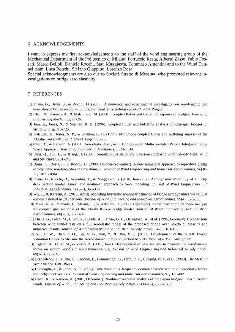
The same quantity is reported in Figure 28 for the point B located on the railway box in

Figure 26:

-500 0 500 1000 1500 2000 2500 3000 35000

2

4

6

8

10

12

14

x [m]

std

σ [

MP

a]

railway box point B

Figure 28. Standard deviation of the stresses at the point B of the different deck sections along the bridge axis.

Wind tunnel results with numerical models are able to drive in the early stage the optimiza-tion of the aerodynamic design of the deck and tower geometry the designer choice for the most important aeroelastic problems that are the aerodynamic stability of the bridge and the VIV of the deck, tower and cables. The most promising solution is therefore analysed most in detail through aeroelastic full bridge models in wind tunnel. The results of the full aeroelastic model are compared with the numerical simulations in order to control all the design procedure.

102

6 ACKNOWLEDGEMENTS

I want to express my first acknowledgements to the staff of the wind engineering group of the Mechanical Department of the Politecnico di Milano: Ferruccio Resta, Alberto Zasso, Fabio Fos-sati, Marco Belloli, Daniele Rocchi, Sara Muggiasca, Tommaso Argentini and to the Wind Tun-nel team: Luca Ronchi, Stefano Giappino, Lorenzo Rosa. Special acknowledgments are also due to Società Stretto di Messina, who promoted relevant in-vestigations on bridge aero elasticity.

7 REFERENCES

[1] Diana, G., Bruni, S., & Rocchi, D. (2005). A numerical and experimental investigation on aerodynamic non linearities in bridge response to turbulent wind. Proceedings oftheEACWE4. Prague.

[2] Chen, X., Kareem, A., & Matsumoto, M. (2000). Coupled flutter and buffeting response of bridges. Journal of Engineering Mechanics, 17-26.

[3] Jain, A., Jones, N., & Scanlan, R. H. (1996). Coupled flutter and buffeting analysis of long-span bridges. J. Struct. Engrg, 716-725.

[4] Katsuchi, H., Jones, N. P., & Scanlan, R. H. (1999). Multimode coupled flutter and buffeting analysis of the Akashi-Kaikyo Bridge. J. Struct. Engrg, 60-70.

[5] Chen, X., & Kareem, A. (2001). Aeroelastic Analysis of Bridges under Multicorrelated Winds: Integrated State-Space Approach. Journal of Engineering Mechanics, 1124-1134.

[6] Ding, Q., Zhu, L., & Xiang, H. (2006). Simulation of stationary Gaussian stochastic wind velocity field. Wind and Structures, 231-243.

[7] Diana, G., Resta, F., & Rocchi, D. (2008, October-November). A new numerical approach to reproduce bridge aerodynamic non-linearities in time domain . Journal of Wind Engineering and Industrial Aerodynamics, 96(10-11), 1871-1884.

[8] Diana, G., Rocchi, D., Argentini, T., & Muggiasca, S. (2010, June-July). Aerodynamic instability of a bridge deck section model: Linear and nonlinear approach to force modeling. Journal of Wind Engineering and Industrial Aerodynamics, 98(6-7), 363-374.

[9] Wu, T., & Kareem, A. (2011, April). Modeling hysteretic nonlinear behavior of bridge aerodynamics via cellular automata nested neural network. Journal of Wind Engineering and Industrial Aerodynamics, 99(4), 378-388.

[10] Minh, N. N., Yamada, H., Miyata, T., & Katsuchi, H. (2000, December). Aeroelastic complex mode analysis for coupled gust response of the Akashi Kaikyo bridge model. Journal of Wind Engineering and Industrial Aerodynamics, 88(2-3), 307-324.

[11] Diana, G., Falco, M., Bruni, S., Cigada, A., Larose, G. L., Darnsgaad, A., et al. (1995, February). Comparisons between wind tunnel tests on a full aeroelastic model of the proposed bridge over Stretto di Messina and numerical results. Journal of Wind Engineering and Industrial Aerodynamics, 54-55, 101-103.

[12] Niu, H. W., Chen, Z. Q., Liu, M. G., Han, Y., & Hua, X. G. (2011). Development of the 3-DOF Forced Vibration Device to Measure the Aerodynamic Forces on Section Models. Proc. of ICWE. Amsterdam.

[13] Cigada, A., Falco, M., & Zasso, A. (2001, June). Development of new systems to measure the aerodynamic forces on section models in wind tunnel testing. Journal of Wind Engineering and Industrial Aerodynamics, 89(7-8), 725-746.

[14] Brancaleoni, F., Diana, G., Faccioli, E., Fiammenghi, G., Firth, P. T., Gimsing, N. J., et al. (2009). The Messina Strait Bridge. CRC Press.

[15] Caracoglia, L., & Jones, N. P. (2003). Time domain vs. frequency domain characterization of aeroelastic forces for bridge deck sections. Journal of Wind Engineering and Industrial Aerodynamics, 91, 371-402.

[16] Chen, X., & Kareem, A. (2001, December). Nonlinear response analysis of long-span bridges under turbulent winds. Journal of Wind Engineering and Industrial Aerodynamics, 89(14-15), 1335-1350.

103

Documents

Wind tunnel tests and numerical approach for long span bridges: the Messina bridgeiawe.org/Proceedings/BBAA7/G.Diana.pdf · 2014-03-07 · Wind tunnel tests and numerical approach