CHAPTER 4

ROOTS OF EQUATIONS

Chapter 3 : TOPIC COVERS

(ROOTS OF EQUATIONS) Definition of Root of Equations

Bracketing Method

•Graphical Method

•Bisection Method

•False Position Method

Open Method

•One-Point Iteration Method

•Newton-Raphson Iteration Method

•Secant Method

Applications in Chemical Engineering

LEARNING OUTCOMES

INTRODUCTION

It is expected that students will be able to:

•Recognize what is the root of equation

•Use bracketing and open methods for root location

•Clarify the concept of convergence/meeting point and

divergence/deviation

CHAPTER 3 : ROOTS OF EQUATIONS

3.1 Introduction

Years ago, you learned to use the quadratic formula;

x = - b [ b2 – 4ac] / 2a - - - - - (3.1)

To solve; f(x) = ax2 + bx + c = 0 - - - - - (3.2)

The values calculated by equation (3.1) are called the “roots” of equation

(3.2). They represent the values of x that make equation (3.2) equal to

zero.

Thus, roots of equations can be defined as “ the value of x that makes f(x) = 0 ” or can be called as the zeros of the equation.

Although the quadratic formula is handy for solving, there are many

other functions/formulas which the root cannot be determined. For

these cases, NM in this chapter provide the efficient answer.

An example where mathematical function (such as quadratic formula)

cannot be used to determine roots of equation is The Newton’s 2nd Law

for the parachutist’s velocity:

v = gm/c (1 – e –(c/m)t ) - - - - - - (3.3)

If the parameters are known, equation (3.3) can be used to predict the

parachutist’s velocity as a function of time.

However, suppose we had to determine the drag coefficient, c for a

parachutist of a given mass to prescribe velocity, v in a set time period,

t.

Although equation (3.3) provides a mathematical representation of the

interrelationship among the model variables & parameters, it cannot be solved for the drag coefficient, c.

The solution to the dilemma is provided by NM for roots of equations.

3.2 Methods to Determine Roots of Equations

A. Bracketing Methods

i. Graphical Method ii. Bisection Method

iii. False-Position Method

B. Open Method

i. Simple Fixed-Point Iteration

ii. Newton-Raphson Method

iii. The Secant Method

C. Engineering Application for Roots of Equations

A. Bracketing Methods

These techniques are called bracketing methods because 2 initial guesses

for the root are required and these guesses must be “bracket”.

i. Graphical Method

“Obtaining an estimate of the root of the equation f(x) = 0 is to make a plot

of the function & observe where it crosses the axis. This point, which

represents the x value for which f(x) = 0, provides a rough approximation

of the root.

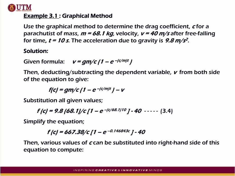
Example 3.1 : Graphical Method

Use the graphical method to determine the drag coefficient, c for a

parachutist of mass, m = 68.1 kg, velocity, v = 40 m/s after free-falling

for time, t = 10 s. The acceleration due to gravity is 9.8 m/s2.

Solution:

Given formula: v = gm/c (1 – e –(c/m)t )

Then, deducting/subtracting the dependent variable, v from both side

of the equation to give:

f(c) = gm/c (1 – e –(c/m)t ) – v

Substitution all given values;

f (c) = 9.8 (68.1)/c [1 – e –(c/68.1)10 ] - 40 - - - - - (3.4)

Simplify the equation;

f (c) = 667.38/c [1 – e –0.146843c ] - 40

Then, various values of c can be substituted into right-hand side of this

equation to compute:

c f(c)

4 34.115

8 17.653

12 6.067

16 -2.269

20 -8.401

These points are plotted in Fig. 3.1. The resulting curve crosses the c axis is between

12 and 16.

Visual inspection (shows in Fig. 3.1) of the plot provides a rough estimate of the

root of 14.75. The validity of the graphical estimate can be checked by substituting

it into equation (3.4) to yield:

f (14.75) = 9.8 (68.1)/14.75 [1 – e –(14.75/68.1)10 ] - 40

= 0.059 (which is close to zero)

It can also be checked by substituting c = 14.75 into given equation (3.3) to give:

v = gm/c (1 – e –(c/m)t ) (given equation)

v = 9.8 (68.1)/14.75 (1 – e –(14.75/68.1)10 ) = 40.059 m/s

which is very close to desire fall velocity of 40 m/s.

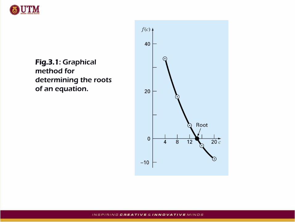
Fig.3.1: Graphical

method for

determining the roots

of an equation.

ii. Bisection Method

When applying graphical method, we observed f(x) has changed sign from +ve to

–ve, where;

f(xl).f(xu) < 0

Then there is at least one real root between xl and xu.

In this method, we dividing halve the interval (xl and xu ) into a number of sub-

intervals. Each sub-interval is to locate the sign changes.

Step of Calculation:

Step 1: Choose lower xl and upper xu such that the function changes sign (+ve and

–ve) over the interval, where this can be checked by ensuring that f(xl ).f(xu ) < 0

Step 2: Estimate the root: xr = (xl + xu ) / 2

Step 3: Make the following evaluations to determine in which subinterval the root

lies:

a. If f(xl ).f(xr ) < 0, root lies in the lower subinterval. Therefore, set xu = xr and return

to step 2.

b. If f(xl ).f(xr ) > 0, root lies in the upper subinterval. Therefore, set xl = xr and return

to step 2.

c. If f(xl ).f(xr ) = 0, the root equals xr ; terminate the computation.

Example 3.2 : Bisection Method

Use bisection to solve the same problem approached graphically in Example 3.1.

Stopping criterion is given as = 0.5%.

Solution:

The first step in bisection is to guess 2 values of the unknown, which in present

problem, c that give values for f(x) with different sign.

Therefore, in 2nd step the initial estimate of the root, xr lies at the midpoint of the

interval values of 12 and 16.

xr = (xl + xu) / 2

xr = (12+ 16) / 2 = 14

This estimate represents a true percent relative error of t = 5.3% [true value of the

root is 14.7802 )

Next we compute the function value at the lower bound and at the midpoint (as trial):

f(12).f(14) = (6.067)(1.569) = 9.517

which is greater than zero, hence no sign change occurs between the lower bound

and the midpoint. Consequently, the root must be located between 14 and 16.

Therefore, redefining the lower bound as 14 and determining a revised root as:

s

Fig.3.2: The Bisection Method for

the first three iterations from

Example 3.2

Fig.3.3:True and

Approximation Errors

of Bisection Method

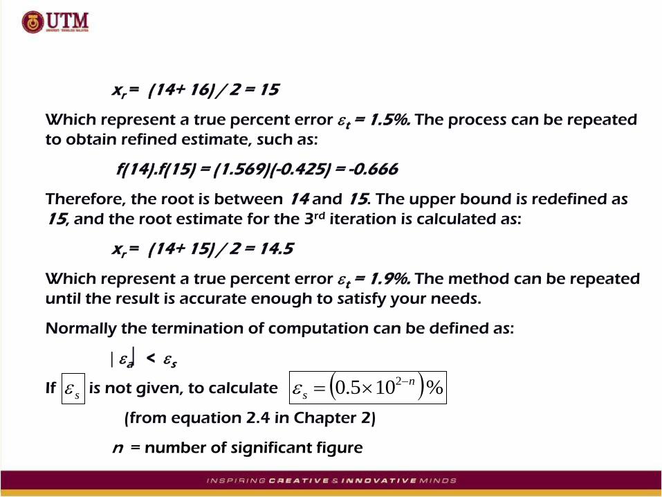
xr = (14+ 16) / 2 = 15

Which represent a true percent error t = 1.5%. The process can be repeated

to obtain refined estimate, such as:

f(14).f(15) = (1.569)(-0.425) = -0.666

Therefore, the root is between 14 and 15. The upper bound is redefined as

15, and the root estimate for the 3rd iteration is calculated as:

xr = (14+ 15) / 2 = 14.5

Which represent a true percent error t = 1.9%. The method can be repeated

until the result is accurate enough to satisfy your needs.

Normally the termination of computation can be defined as:

a < s

If is not given, to calculate

(from equation 2.4 in Chapter 2)

n = number of significant figure

% 105.0 2 n

s

s

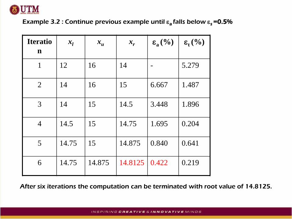
Iteratio

n

xl xu xr a (%)

t (%)

1 12 16 14 - 5.279

2 14 16 15 6.667 1.487

3 14 15 14.5 3.448 1.896

4 14.5 15 14.75 1.695 0.204

5 14.75 15 14.875 0.840 0.641

6 14.75 14.875 14.8125 0.422 0.219

Example 3.2 : Continue previous example until a falls below s =0.5%

After six iterations the computation can be terminated with root value of 14.8125.

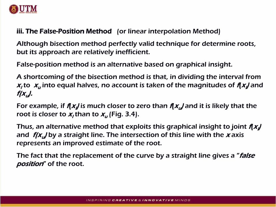
iii. The False-Position Method (or linear interpolation Method)

Although bisection method perfectly valid technique for determine roots,

but its approach are relatively inefficient.

False-position method is an alternative based on graphical insight.

A shortcoming of the bisection method is that, in dividing the interval from

xl to xu into equal halves, no account is taken of the magnitudes of f(xl) and f(xu).

For example, if f(xl) is much closer to zero than f(xu) and it is likely that the

root is closer to xl than to xu (Fig. 3.4).

Thus, an alternative method that exploits this graphical insight to joint f(xl) and f(xu) by a straight line. The intersection of this line with the x axis

represents an improved estimate of the root.

The fact that the replacement of the curve by a straight line gives a “false position” of the root.

Fig.3.4: False

Position Method

Fig.3.5:Comparison of

relative error of

Bisection and False-

Position Method

f(xu)

f(xl)

xl

xu

x

f(x)

xr

To determine the formula for the false-position method:

Using similar triangles, (From Fig. 3.4) the intersection of the straight line with

the x axis can be estimated as;

- - - - - (3.5)

The equation above can be solves;

- - - - - (3.6)

Equation (3.6) is called as False-Position Formula.

f (xl )

(xr xl )f (xu)

(xr xu)

xr xu f (xu).(xl xu)

f (xl ) f (xu)

Example 3.3: False-Position Method

Use the false-position method to determine the root of the same equation

investigated in Example 3.1

Solution: As in Example 3.2, the computation guesses of xl = 12 and xu = 16

(true value of the root is 14.7802)

First iteration: xl =12 f(xl ) = 6.0699

xu = 16 f(xu ) = -2.2688

xr = 16 – (-2.2688)(12-16)/(6.0669)-(-2.2688)

= 14.9113 (true relative error 0.89%)

Therefore, the root lies in the first subinterval (xl) , and xr becomes the upper

limit for the next iteration, xu = 14.9113

Second iteration: xl =12 f(xl ) = 6.0699

xu = 14.9113 f(xu ) = -0.2543

xr = 14.9113–(-0.2543)(12-14.9113)/(6.0669)-(-0.2543)

= 14.7942 (approximate relative error 0.79% and

true error 0.09%)

Additional iteration can be performed to refine the estimate of the

roots.

Bisection Algorithm Results

Example 4.4 with s = 0.5%

Iter xl xu xr Ea Et

1 12.00 16.000 14.0000 - 5.279

2 14.00 16.000 15.0000 6.667 1.487

3 14.00 15.000 14.5000 3.448 1.896

4 14.50 15.000 14.7500 1.695 0.205

5 14.75 15.000 14.8750 0.840 0.641

6 14.75 14.875 14.8125 0.422 0.218

False Position Algorithm Results

Example 4.4 with s = 0.5%

Iter xl xu xr Ea Et

1 12.00 16.000 14.9113 - 0.887

2 12.00 14.911 14.7942 0.792 0.094

3 12.00 14.794 14.7817 0.085 0.010

B. Open Method

For the bracketing methods, the root is located within an interval prescribed by a

lower and an upper bound. Repeated application of these methods always results in

closer estimates of the true value of the root (convergent : move closer to the truth as

the computation progresses)

In contrast, the open methods are based on formulas that require only a single

starting value of x or 2 starting values that do not necessarily bracket the root.

However, when the open methods converge they usually do so much quickly than

the bracketing method.

i. Simple Fixed-Point Iteration

Rearranging the function f(x) = 0 so that x is on the left-hand side of the equation:

x =g (x) - - - - - - (3.7)

This transformation can be accomplished either by algebraic manipulation or by

simply adding x to both sides of the original equation. For example;

x2 – 2x + 3 = 0

Can be simply manipulated to yield:

x = (x2 + 3) / 2

Another example: sin x = 0

Could be put into the form of equation (3.7) by adding x to both sides to

yield:

x = sin x + x

The utility of equation (3.7) is that provides a formula to predict a new

value of x as a function of an old value of x. Thus, given an initial guess at

the root xi, equation (3.7) can be used to compute a new estimate xi+1 as

expressed by the iterative formula;

xi+1 = g(xi) - - - - - - - (3.8)

The approximate error for this equation can be determined using the error

estimator as discussed in previous Chapter 2, which is;

%1001

1

i

iia

x

xx

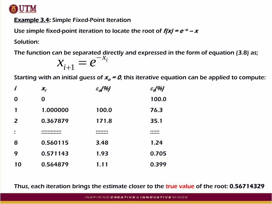
Example 3.4: Simple Fixed-Point Iteration

Use simple fixed-point iteration to locate the root of f(x) = e -x – x

Solution:

The function can be separated directly and expressed in the form of equation (3.8) as;

ix

i ex

1

Starting with an initial guess of xo = 0, this iterative equation can be applied to compute:

i xi a(%) t(%)

0 0 100.0

1 1.000000 100.0 76.3

2 0.367879 171.8 35.1

: ::::::::::::: :::::::: ::::::

8 0.560115 3.48 1.24

9 0.571143 1.93 0.705

10 0.564879 1.11 0.399

Thus, each iteration brings the estimate closer to the true value of the root: 0.56714329

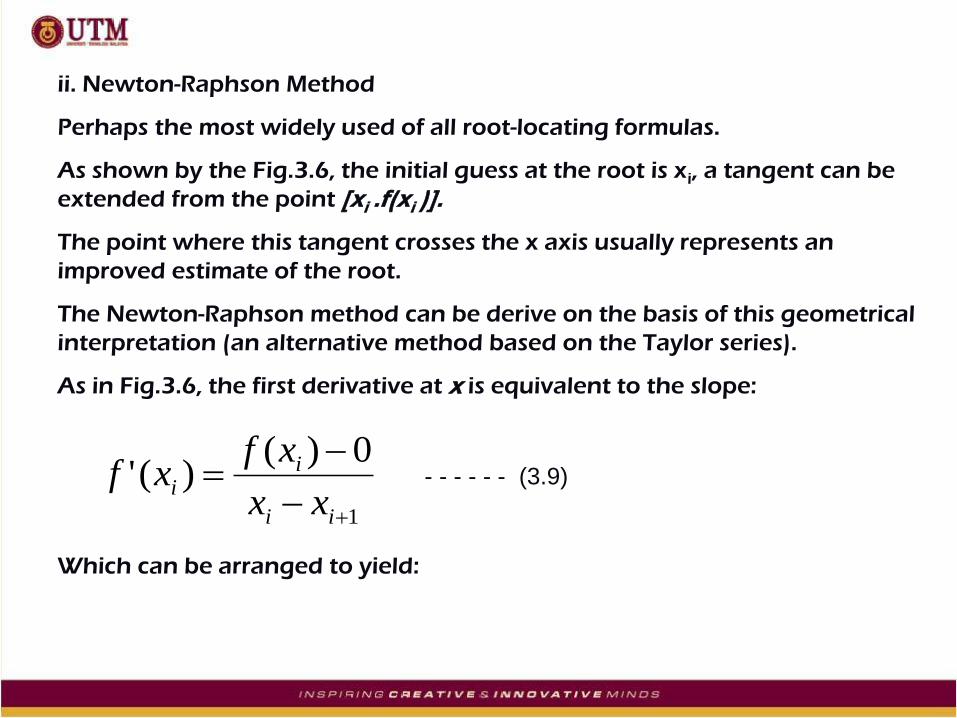
ii. Newton-Raphson Method

Perhaps the most widely used of all root-locating formulas.

As shown by the Fig.3.6, the initial guess at the root is xi, a tangent can be

extended from the point [xi .f(xi )].

The point where this tangent crosses the x axis usually represents an

improved estimate of the root.

The Newton-Raphson method can be derive on the basis of this geometrical

interpretation (an alternative method based on the Taylor series).

As in Fig.3.6, the first derivative at x is equivalent to the slope:

1

0)()('

ii

ii

xx

xfxf - - - - - - (3.9)

Which can be arranged to yield:

)('

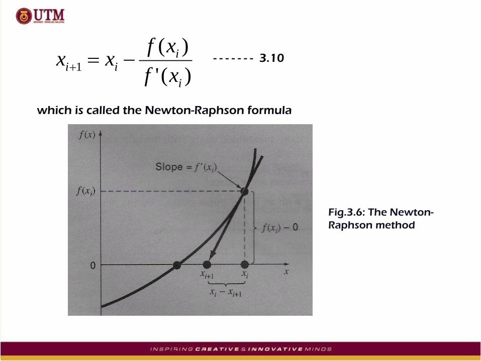
)(1

i

iii

xf

xfxx

- - - - - - - 3.10

which is called the Newton-Raphson formula

Fig.3.6: The Newton-

Raphson method

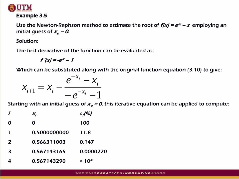
Example 3.5

Use the Newton-Raphson method to estimate the root of f(x) = e-x – x employing an

initial guess of xo = 0.

Solution:

The first derivative of the function can be evaluated as:

f ’(x) = -e-x – 1

Which can be substituted along with the original function equation (3.10) to give:

11

i

i

x

i

x

iie

xexx

Starting with an initial guess of xo = 0, this iterative equation can be applied to compute:

i xi t(%)

0 0 100

1 0.5000000000 11.8

2 0.566311003 0.147

3 0.567143165 0.0000220

4 0.567143290 < 10-8

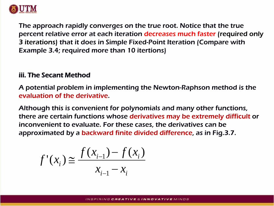
The approach rapidly converges on the true root. Notice that the true

percent relative error at each iteration decreases much faster (required only

3 iterations) that it does in Simple Fixed-Point Iteration (Compare with

Example 3.4; required more than 10 itertions)

iii. The Secant Method

A potential problem in implementing the Newton-Raphson method is the

evaluation of the derivative.

Although this is convenient for polynomials and many other functions,

there are certain functions whose derivatives may be extremely difficult or

inconvenient to evaluate. For these cases, the derivatives can be

approximated by a backward finite divided difference, as in Fig.3.7.

ii

iii

xx

xfxfxf

1

1 )()()('

Fig.3.7: The

Scan Method

plot.

From the backward finite divided difference substituted into equation (3.10)- The

Newton-Raphson Method equation: To yield the following iterative equation:

)()(

))((

1

11

ii

iiiii

xfxf

xxxfxx

- - - - 3.11 This formula is

for the Secant

Method.

Notice that the Scant Method requires two initial estimates of x. However,

because f(x) is not required to change signs between the estimates, it is not

classified as a bracketing method.

Example 3.6: The Scant Method

Use the scant method to estimate the root of f(x) = e-x – x. Start with initial

estimates of x-1 = 0 and xo = 1.0.

Solution:

Recall that the true root is 0.56714329…..

First iteration:

x-1 = 0 f(x-1) = 1.00000

xo = 1 f(xo) = -0.63212

x1 = 1 – [-0.63212(0 – 1) / 1 – (-0.63212)] = 0.61270

t = 8.0%

)()(

))((

1

11

ii

iiiii

xfxf

xxxfxx

Second iteration:

xo = 1 f(xo) = -0.63212

x1 = 0.61270 f(x1) = -0.07081

(Note that both estimates are now on the same side of the root.)

x2 = 0.61270 –

[-0.07081(1 – 0.61270) / -0.63212 – (-0.07081)]

= 0.56384

t = 0.58%

Third iteration:

x1 = 0.61270 f(xo) = -0.07081

x2 = 0.56384 f(x1) = 0.00518

x3 = 0.56384 –

[0.00518(0.61270-0.56384) / -0.07081 – (-0.00518)]

= 0.56717

t = 0.0048%

Problems (Bracketing Method)

5.1 Determine the real roots of f(x) = -0.4x2 + 2.2x + 4.7;

a. Graphically

b. Using the quadratic formula

c. Using three iterations of Bisection Method to determine the highest

root. Employ guesses of xl=5 and xu=10. Compute the estimated error

a and the true error t after each iteration.

5.4 Determine the real roots of;

f(x) = -11 – 22x +17x2 – 2.5x3:

a. Graphically.

b. Using the False-Position Method with a value of s corresponding to

three significant figures to determine the lowest root.

5.6 Determine the real root of ln x2 = 0.7 :

a. Graphically.

b. Using three iterations of the Bisection Method, with initial guesses of xl = 0.5 and

xu = 2.

c. Using three iterations of the False-Position Method, with the same initial guesses

as in (b).

5.7 Determine the real root of f(x) = (0.9 – 0.4x) / x :

a. Analytically.

b. Graphically.

c. Using three iterations of the False-Position Method and initial guesses of 1 and 3.

Compute the approximate error a and the true error t after each iteration.

5.12 The velocity v of a falling parachutist with a drag coefficient c = 14kg/s, compute

the mass m so that the velocity is v = 35m/s at t = 7s. Use the False-Position

Method to determine m to a level of s=0.1%.

Problems (Open Method)

6.1 Use simple Fixed-Point iteration to locate the root of:

xxxf )sin()(

Use an initial guess of xo = 0.5 and iterate until a 0.01%

6.3 determine the real roots of ;

f(x) = -2.0 + 6x – 4x2 + 0.5x3 :

a. Graphically.

b. Using the Newton-Raphson Method to within a=0.01%

6.5 Determine the lowest real root of ;

f(x) = -11 –22x + 17x2 – 2.5x3 :

a. Graphically.

b. Using the Secant Method to a value of s corresponding to three significant

figures.

Solution

5.1 (a) Given equation : f(x) = -0.4x2 + 2.2x + 4.7

Guess the x values so, give f(x) = 0;

x f(x)

-2 -1.3

-1 2.1

0 4.7

1 6.5

2 7.5

4 7.1

6 3.5

8 -3.3

10 -13.3

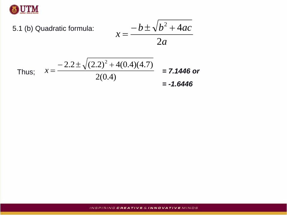
5.1 (b) Quadratic formula:

a

acbbx

2

42

Thus; )4.0(2

)7.4)(4.0(4)2.2(2.2 2 x = 7.1446 or

= -1.6446

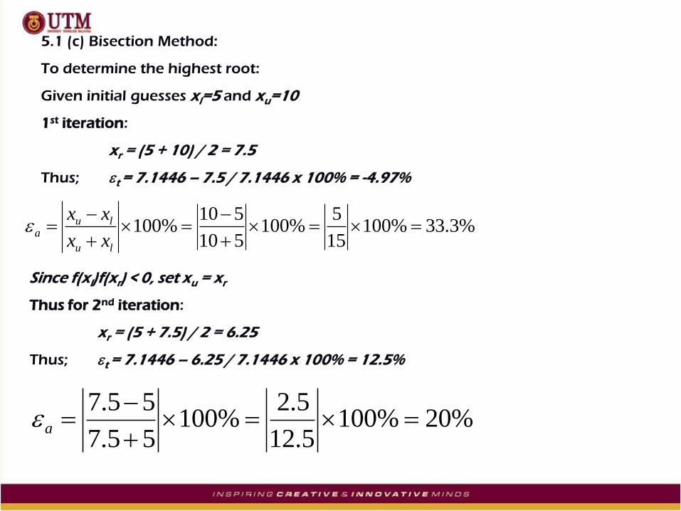
5.1 (c) Bisection Method:

To determine the highest root:

Given initial guesses xl=5 and xu=10

1st iteration:

xr = (5 + 10) / 2 = 7.5

Thus; t = 7.1446 – 7.5 / 7.1446 x 100% = -4.97%

%3.33%10015

5%100

510

510%100

lu

lua

xx

xx

Since f(xl)f(xr) < 0, set xu = xr

Thus for 2nd iteration:

xr = (5 + 7.5) / 2 = 6.25

Thus; t = 7.1446 – 6.25 / 7.1446 x 100% = 12.5%

%20%1005.12

5.2%100

55.7

55.7

a

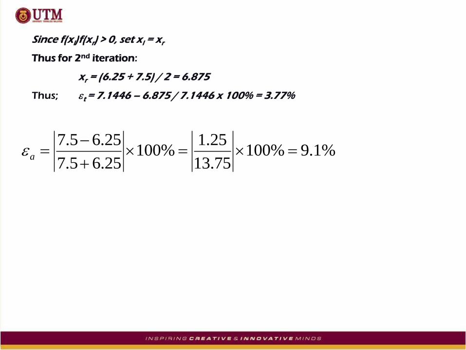
Since f(xl)f(xr) > 0, set xl = xr

Thus for 2nd iteration:

xr = (6.25 + 7.5) / 2 = 6.875

Thus; t = 7.1446 – 6.875 / 7.1446 x 100% = 3.77%

%1.9%10075.13

25.1%100

25.65.7

25.65.7

a

C. Engineering Applications: Roots of Equations

The purpose of this chapter is to use the numerical procedure as discussed

previously to solve actual engineering problems.

Numerical techniques are important for practical applications because

engineers frequently encounter problems that cannot be approached using

analytical techniques.

In the example below is taken from chemical engineering, provides an

excellent example of how root-location method allow you to use realistic

formulas in engineering practice.

Example 3.7: Ideal and Non-Ideal Gas Law

Background: The ideal gas law is given by

pV = nRT - - - - - (3.12)

where; p = absolute pressure V = volume

n = number of moles T = temperature

R = universal gas constant

Although this equation is widely used by engineers and scientists, it is accurate over

only a limited ranges of pressure and temperature.

Furthermore the equation is more appropriate for some gases than for others.

An alternative equation of state for gases is given by:

RTbvv

ap

2- - - - - - (3.13)

known as the van der Walls equation.

where;

v = V/n is the molal volume

a and b = empirical constants that depend on the particular gas

Situation/Problem Given:

A chemical engineering design project requires that you accurately estimate the molal

volume (v) of both carbon dioxide and oxygen for a number of different temperature

and pressure combinations so that appropriate containment vessels can be selected.

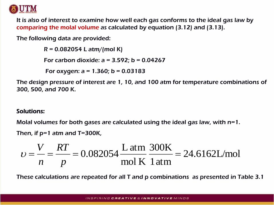
It is also of interest to examine how well each gas conforms to the ideal gas law by

comparing the molal volume as calculated by equation (3.12) and (3.13).

The following data are provided:

R = 0.082054 L atm/(mol K)

For carbon dioxide: a = 3.592; b = 0.04267

For oxygen: a = 1.360; b = 0.03183

The design pressure of interest are 1, 10, and 100 atm for temperature combinations of

300, 500, and 700 K.

Solutions:

Molal volumes for both gases are calculated using the ideal gas law, with n=1.

Then, if p=1 atm and T=300K,

These calculations are repeated for all T and p combinations as presented in Table 3.1

L/mol6162.24atm 1

300K

K mol

atm L082054.0

p

RT

n

V

Table 3.1: Computations of molal volume, v

Temperature Pressure molal volume molal volume molal volume

K atm ideal gas law van der Wall van der Wall

(L/mol) CO2 (L/mol) (O2 L/mol)

300 1 24.6162 24.5126 24.5928

10 2.4616 2.3545 2.4384

100 0.2462 0.0795 0.2264

500 1 41.0270 40.9821 41.0259

10 4.1027 4.0578 4.1016

100 0.4103 0.3663 0.4116

700 1 57.4378 57.4179 57.4460

10 5.7438 5.7242 5.7521

100 0.5744 0.5575 0.5842

While, the computation of molal volume, v from the van der Waals equation

can be accomplished using any the NM for finding roots of equations

discussed in Chapter 3;

Thus, the equation (3.13) becomes;

- - - - - (3.14)

In this case, the derivative of f(v) is easy to determine and the Newton-

Raphson method is convenient and efficient to implement.

The derivative of f(v) with respect to v is given by:

The Newton-Raphson method is described by equation (3.10):

RTbvv

apvf

2)(

)('

)(1

i

iii

vf

vfvv

32

2)('

v

ab

v

apvf

From this equation, root of equation can be estimated.

For example, using the initial guess of 24.6162, the molal volume of CO2 at

300K and 1 atm is computed as 24.5126 L.mol.

This result was obtained after just 2 iterations and has an a less than 0.001 %.

The rest of computations can be estimated by using similar method and all

results are presented in Table 3.1.

PLEASE DO YOUR HOMEWORK TO PRODUCE ALL RESULTS AS

PRESENTED IN TABLE 3.1.

YOU ARE SUGGESTED TO TRY OTHER METHODS AS WELL TO

DETERMINE THE ROOTS OF EQUATIONS !!!!!

END

OF

CHAPTER 3