Embed Size (px)
Citation preview

1/56
Instructor Tao, Wen-Quan
CFD-NHT-EHT Center
Key Laboratory of Thermo-Fluid Science & Engineering
Xi’an Jiaotong University
Xi’an, 2017-Oct-11
Numerical Heat Transfer (数值传热学)
Chapter 4 Numerical Solution of Diffusion Equation and its Applications(2)

3/56
4.1 1-D Heat Conduction Equation
4.2 Fully Implicit Scheme of Multi-dimensional
Heat Conduction Equation
4.3 Treatments of Source Term and B.C.
Contents
4.4 TDMA & ADI Methods for Solving ABEs
4.6 Fully Developed HT in Rectangle Ducts
4.5 Fully Developed HT in Circular Tubes

4/56
4.4 TDMA & ADI Methods for Solving ABEs
4.4.1 TDMA algorithm (算法) for 1-D conduction
problem
4.4.2 ADI method for solving multi-
dimensional problem
1. Introduction to the matrix of 2-D problem
1.General form of algebraic equations of 1-D conduction problems
2. ADI iteration of Peaceman-Rachford
2.Thomas algorithm
3.Treatment of 1st kind boundary condition

5/56
4.4 TDMA & ADI Methods for Solving ABEqs
4.4.1 TDMA algorithm for 1-D conduction problem
1.General form of algebraic equations. of 1-D
conduction problems
The ABEqs for
steady and unsteady
(f>0) problems take
the form
The matrix (矩阵) of
the coefficients is a tri-
diagonal (三对角) one .
P P E E W Wa T a T a T b
Three unknowns

6/56
2. Thomas algorithm(算法)
Rewrite above equation:
End conditions:i=1, Ci=0; i=M1, Bi=0
(1) Elimination (消元)-Reducing the unknowns at
each line from 3 to 2
Assuming the eq. after
elimination as
1 1, 1,2,..... 1
i i i i i i iAT BT CT D i M
(a)
1 1 1i i i iT P T Q
Coefficient has been treated to 1.
(b)
The numbering method of W-P-E is humanized
(人性化), but it can not be accepted by a computer!

7/56
The purpose of the elimination procedure is to find
the relationship between Pi , Qi with Ai , Bi , Ci , Di:
Multiplying Eq.(b) by Ci, and adding to Eq.(a):
1 1i i i i i i iAT BT CT D
(a)
(b) 1 1 1i iii ii iT PC T QC C
1i i i i iAT C P T 1 1i i i i iBT D C Q
11
1 1
( )i i i ii i
i i i i i i
B D C QT T
A C P A C P
1 1 1i i i iT P T Q Comparing with
Yielding

8/56
1
;ii
i i i
BP
A C P
1
1
;i i ii
i i i
D C QQ
A C P
The above equations are recursive -i.e.,
In order to get Pi , Qi , P1 and Q1 must be known.
1 1, 1,2,..... 1
i i i i i i iAT BT CT D i M
(a)
End condition:i=1, Ci=0; i=M1, Bi=0
In order to get P1,Q1,use Eq.(a)
Applying Eq.(a) to i=1, and comparing it with
Eq. (b) , the expressions of P1,Q1 can be
9/56
11, 0,i C 1 1 1 2 1AT BT D
1 11 2
1 1
B DT T
A A 1
1
1
;B
PA
11
1
DQ
A
(2) Back substitution(回代)-Starting from M1 via
Eq.(b) to get Ti sequentially(顺序地)
1 1 1 1 1 ,M M M MT P T Q
End condition:
i=M1, Bi=0
1 1M MT Q
1
;ii
i i i
BP
A C P
10
MP
1 1 1i i i iT P T Q
obtained:
to get: 1 1 2 1,...... , .MT T T
10/56
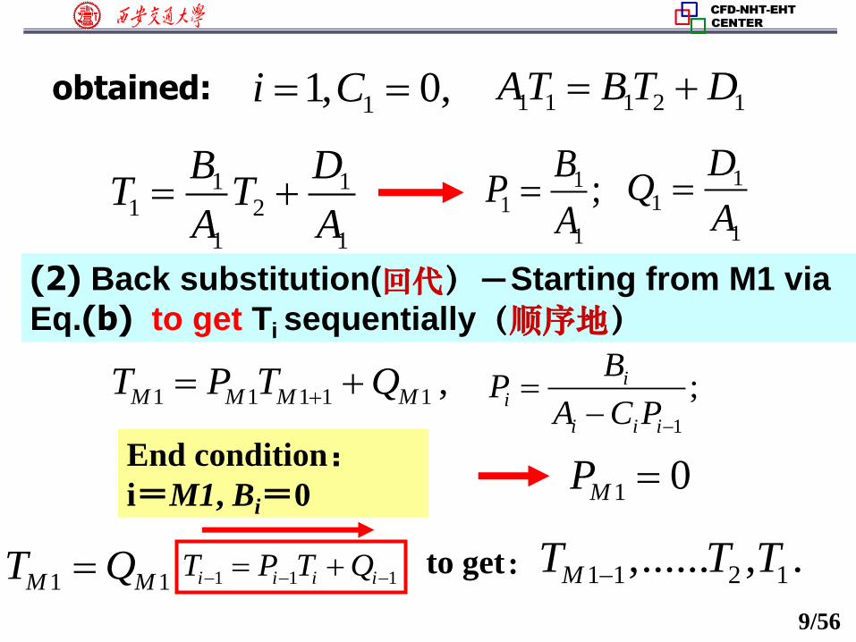
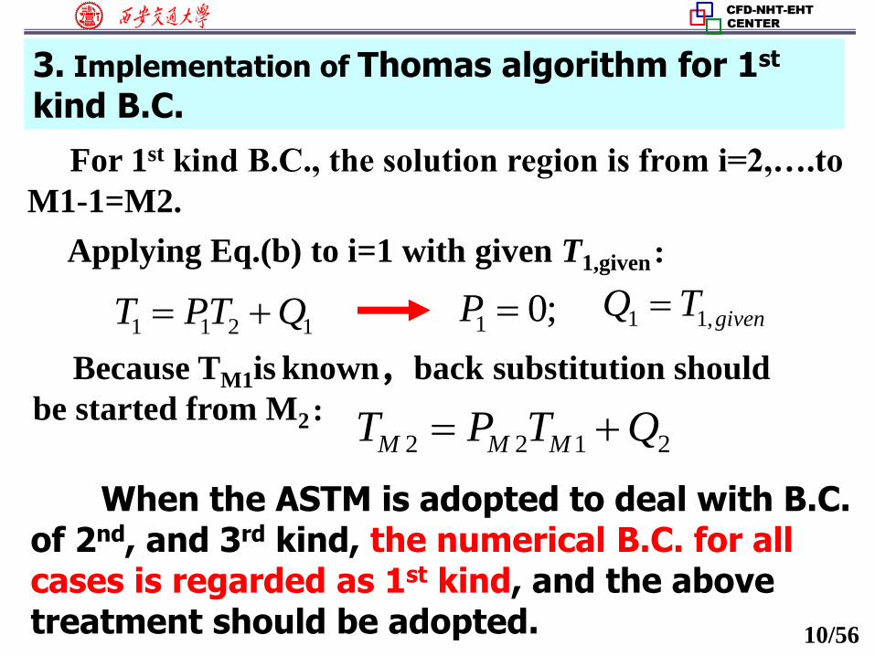
3. Implementation of Thomas algorithm for 1st kind B.C.
For 1st kind B.C., the solution region is from i=2,….to
M1-1=M2.
Applying Eq.(b) to i=1 with given T1,given:
1 1 2 1T PT Q 1 0;P 1 1,givenQ T
Because TM1is known,back substitution should
be started from M2: 2 2 1 2M M MT P T Q
When the ASTM is adopted to deal with B.C. of 2nd, and 3rd kind, the numerical B.C. for all cases is regarded as 1st kind, and the above treatment should be adopted.

11/56
4.4.2 ADI method for solving multi-dimensional
problem
1. Introduction to the matrix of 2-D problem
P E W
N
S S
W
P
N
E
1-D storage (一维存储)of variables and its relation to
matrix coefficients

12/56
(1) Penta-diagonal algorithm(PDMA,五对角阵算法)
(2) Alternative(交替的)-direction Implicit (ADI,
交替方向隐式方法)
2. 3-D Peaceman-Rachford ADI method
Dividing t into three uniform parts
In the 1st / 3t implicit in x direction,
and explicit in y, z directions;
In the 2nd and 3rd implicit in / 3t
y, z direction, respectively.
2-D ADI
Numerical methods for solving ABEqs. of 2-D problems.
t

13/56
Set ui,j,k , vi,j,k the temporary(临时的) solutions at
two sub-time levels
-CD for 2nd derivative at n time level in x
direction
2
, ,
n
x i j kT
, ,
, ,
, , 2 2 2
, , , ,( )/ 3
i j
n
i j k n n
x y i j k z i j k
k
i j k
Ta T T
t
uu
1st sub-
time level
2nd sub-
time level: , 2, 2
, , ,
, ,
, , ,
2( )
/ 3
n
i j k
ix
i j k
i j k i j kyj k z
ua
t
vvu u
3rd sub-
time level , ,
,
1
, 2 2 2,
,, , ,,
1( )
/ 3
n
i j k n
i j k i j k
n
i j k n
y i j kx z
TTa v v
t
v

14/56
Stability condition by von Neumann method:
2 2 2
1 1 1( ) 1.5a t
x y z
Is the allowed maximum time step three times of
1-D case?
3. Two “ADI” methods: ADI-implicit(交替方向隐式)
for transient problems and ADI-iteration(交替方向迭代)
multi-dimensional problems. They are very similar.
Actually, No!
For 2-D case P-R method is absolutely stable.

15/56
5 FDHT in Circular Tubes
4.5.2 Physical and Mathematical Models
4.5.3 Governing equations and their non- dimensional forms
4.5.4 Conditions for unique solution
4.5.5 Numerical solution method
4.5.6 Treatment of numerical results
4.5.7 Discussion on numerical results
4.5.1 Introduction to FDHT in tubes and ducts

16/56
4.5.1 Introduction to FDHT in tubes and ducts
1. Simple fully developed heat transfer
Physically:Velocity components normal to flow
direction equal zero; Fluid dimensionless
temperature distribution is independent on(无关)
the position in the flow direction
Mathematically:Both dimensionless momentum and
energy equations are of diffusion type.
Present chapter is limited to simple cases.
4.5 Fully Developed HT in Circular Tubes

17/56
FDHT in straight duct
is an example of simple cases.
2. Complicated FDHT
In the cross section normal to flow direction there
exist velocity components , and the dimensionless
temperature depends on the axial position, often
exhibits periodic (周期的)character. The full Navier-
Stokes equations must be solved。
This subject is discussed in Chapter 11 of the textbook.
,
,
( ) 0w m
w bm
T
T
T
x T

18/56
Examples of complicated FDHT
Tube bundle (bank) (管束)
Fin-and-tube heat exchanger Louver fin (百叶窗翅片)

19/56
3. Collection of partial examples
No Cross section B. Condition Refs
Table 4-5 Numerical examples of simple FDHT
See pp. 106-109 for details

20/56
4.5.2 Physical and mathematical models
A laminar flow in a long tube is cooled (heated) by
an external fluid with temp. and heat transfer
coefficient . Determine the heat transfer coefficient
and Nusselt number in the FDHT region.
T
eh

21/56
1.Simplification (简化) assumptions
(1) Thermo-physical properties are constant ;
(2) Axial heat conduction in the fluid is neglected
(5) Wall thermal resistance is neglected;
(3) Viscous dissipation (耗散)is neglected;
(4) Natural convection is neglected;
(6) The flow is fully developed:
22[1 ( ) ]; 0
m
u rv
u R

22/56
2. Mathematical formulation (描述)
(1)Energy equation
1( ) ( ) ( )
p T
T T T Tc u v r S
x r r r r x x
Cylindrical coordinate, symmetric temp. distribution,
and no natural convection (A4):
FD flow (A6)
No axial cond.(A2)
1( )p
T Tc u r
x r r r
2-D parabolic eq.!
Type of eq.?
No dissipation(A3)

23/56
(2)Boundary condition
0, 0T
rr
(Symmetric condition);
, ( )e
TT
rR Tr h
(External convective condition!)
No wall thermal
resistance(A5), tube
outer radius =R;。
Internal fluid thermal conductivity
External (外部)convective
heat transfer

24/56
4.5.3 Governing eqs. and dimensionless forms
From FD condition a dimensionless temp. can be
introduced, transforming the PDE to ordinary eq..
Defining b
T T
T T
b
T T
T T
T T
T T
Then: ( ) ;b
T T T T
b bT T dT
x x dx
Defining dimensionless space and “time” coordinates:
;r
R
xX
R Pe
2 2p m mR c u Ru
Pea
Constant properties(A 1)

25/56
Energy eq. can be rewritten as:
/ 1 1( ) / ( )
2
b
b m
dT dX d d u
T T d d u
= 0
is called eigenvalue (特征值)
Dependent on X only Dependent on only

26/56
Following ordinary PDE for the dimensionless
temperature. eq. can be obtained
1 1( ) /( )
2 m
d d u
d d u
The original two B.Cs. are transformed (转换成) into:
0, 0;d
d
( )
1, ( )
( )
eb
b
Td
h R T T
r
T
d
T
R
T
T T
1) w
dBi
d
(a)
(b)
(c) Question:whether from Eqs.(a)-(c) a unique (唯一的) solution can be obtained?

27/56
4.5.4 Analysis of condition for unique solution
For the above mathematical formulation there exists
an uncertainty (不确定性)of being able to be
multiplied by a constant for its solution.
Because of the homogeneous (齐次性) character :
Every term in the differential equation contains a
linear part of dependent variable or its 1st/2nd derivative.
1 1( ) /( )
2 m
d d u
d d u
1 1( ) ( )
2 m
d d u
d d u
In addition, the given B.Cs. are also homogeneous:
0, 0;d
d
1) w
dBi
d
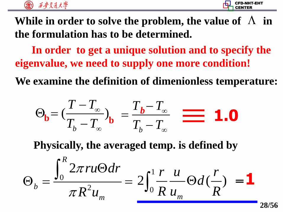
28/56
While in order to solve the problem, the value of in
the formulation has to be determined.
In order to get a unique solution and to specify the
eigenvalue, we need to supply one more condition!
We examine the definition of dimenionless temperature:
( )b
T T
T T
Physically, the averaged temp. is defined by
0
2
2R
b
m
ru dr
R u
=1
b
T T
T T
b b b 1.0
1
02 ( )
m
r u rd
R u R

29/56
Thus the complete formulation is:
1 1( ) ( ) 0
2 m
d d u
d d u
(a)
0, 0;d
d
(b)
1) w
dBi
d
(c)
1
01/ 2
m
ud
u
(d)
Non-homogeneous term!

30/56
4.5.5 Numerical solution method
This is a 1-D conduction equation with a source term!
2 m
u
u
,whose value should be determined during the
solution process iteratively.
Patankar-Sparrow proposed following
(1)Let
Because of the homogeneous character, the form of
the equation is not changed only replacing by .
。
1 1( ) ( ) 0
2 m
d d u
d d u
numerical solution method:

31/56
1 1( ) ( ) 0
2 m
d d u
d d u
(a)
0, 0;d
d
(b)
1) w
dBi
d
(c)
1
01/ 2
m
ud
u (d)
Non-homogeneous term
1
01/(2 )
m
ud
u It can be used to iteratively
determine the eigenvalue.

32/56
(3)Solving an ordinary differential eq. with a source
term to get an improved
(4)Repeating the above procedure until:
(2)Assuming an initial field * , get *
*
,
3 610 ~ 10
This iterative procedure is easy to approach convergence:
1
2 m
uS
u
2
12
0
(1 )
4 (1 ) d
1
0
( / )
4 ( / )
m
m
u u
u u d
1
01/(2 )
m
ud
u

33/56
4.5.6 Treatment of numerical results
Two ways for obtaining heat transfer coefficient:
1. From solved temp. distribution using Fourier’s law of
heat conduction and Newton’s law of cooling:
, ( )w b
Tr R h T T
r
1)r R
w b
T
rh
T T
, ( )e
TT
rR Tr h
Different from
Boundary condition
exists in both numerator and denominator, thus
only the distribution, rather than absolute value will
affect the source term.
For inner fluid
34/56
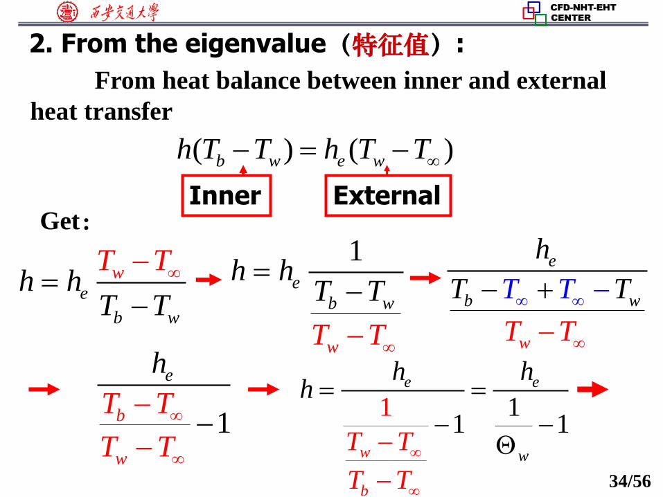
2. From the eigenvalue(特征值):
From heat balance between inner and external
heat transfer
( ) ( )b w e wh T T h T T
Inner External Get:
w
e
b w
T Th h
T T
1w
e
bT T
T
h
T
w
e
b wT T
T T
T
h
T
1 11 1
e e
ww
b
T T
T
h
T
h h
1e
b w
w
h hT T
T T

35/56
1
e w
w
h
1
2 w
w
ehR
1
2 w
w
Bi
, the corresponding
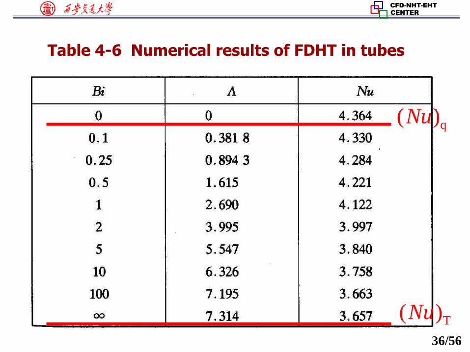
4.5.7 Discussion on numerical results
From the specified values Bi
=1 1
1
e e w
w
w
h hh
eigenvalues, , can be obtained. Thus it is not
necessary to find the 1st derivative at the wall
of function for determining Nusselt number.
2RhNu

37/56
From definition
Bi effect: 1. e
RhBi
,Bi
0e
h
External heat transfer is very
This is corresponding to constant wall temp condition,
Thus Nu=3.66
0,Bi Is this adiabatic? No!
eh
Product of very small HT coefficient and very large temp. difference makes heat flux almost constant.
eq h T const
strong,the wall temp. approaches fluid temp.

38/56
510 ,
Bi=0 by progressively decreasing Bi:
Double decision (双精度)must be used for Computation:
Bi= 6
107
,10 .....
Bi= 0.1, 0.01, 0.0001, 0.001, 0.00001,
1
2,w
w
BiNu
0, 0, 1wBi
0
0
2. Computer implementation of Bi and Bi 0
Bi by progressively (逐渐地)
increasing Bi:

39/56
4.6 Fully Developed HT in Rectangle Ducts
4.6.1 Physical and mathematical models
4.6.2 Governing eqs. and their dimensionless forms
4.6.3 Condition for unique solution
4.6.4 Treatment of numerical results
4.6.5 Other cases(20171011)

1. TDMA solution algorithm for 1-D problem
Brief review of 2017-10-11 lecture key points
2. ADI method for solving 2-D unsteady problem
(1) Elimination (消元)-Reducing the unknowns at
each line from 3 to 2
1
;ii
i i i
BP
A C P
1
1
;i i ii
i i i
D C QQ
A C P
1
1
1
;B
PA
11
1
DQ
A
1 1 1i i i iT P T Q 1 1i i i i i i iAT BT C T D
recursive
Dividing t into two uniform parts;In the 1st / 2t
(2) Back substitution(回代)-Starting from the last
node via Eq.(b) to get Ti sequentially
(a) (b)
40/56
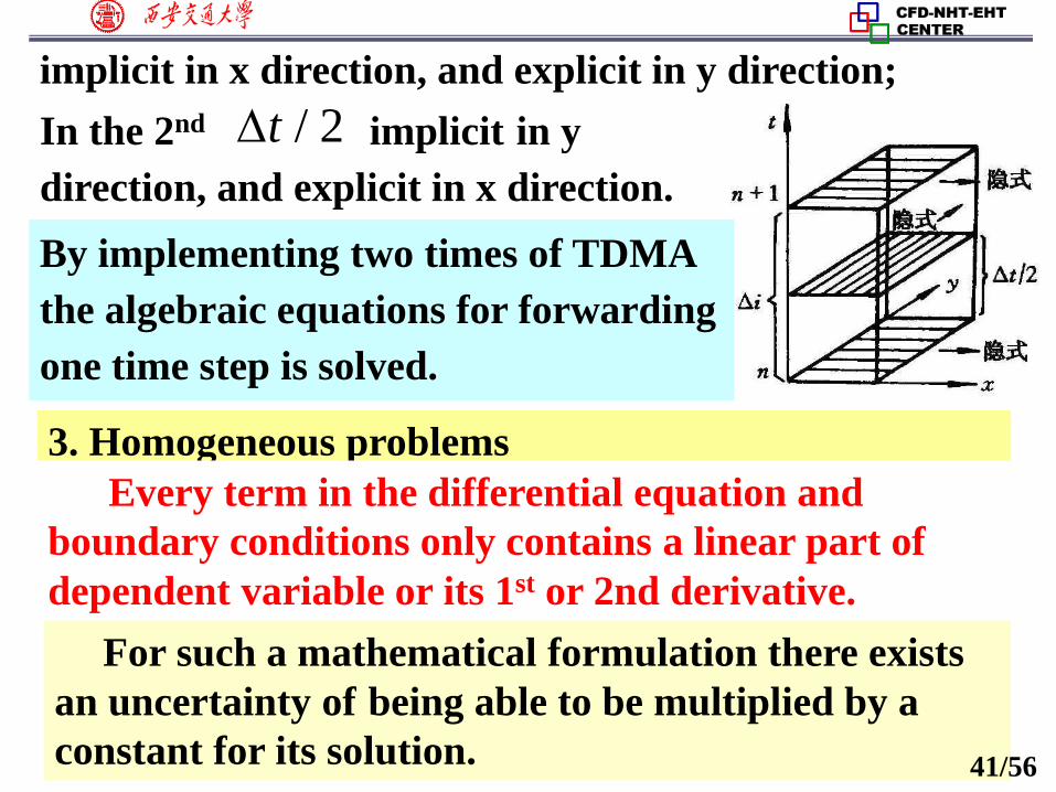
3. Homogeneous problems
In the 2nd implicit in y
direction, and explicit in x direction.
/ 2t
By implementing two times of TDMA
the algebraic equations for forwarding
one time step is solved.
Every term in the differential equation and
boundary conditions only contains a linear part of
dependent variable or its 1st or 2nd derivative.
For such a mathematical formulation there exists
an uncertainty of being able to be multiplied by a
constant for its solution.
implicit in x direction, and explicit in y direction;
41/56

4.6 Fully Developed HT in Rectangle Ducts
4.6.1 Physical and mathematical models
Fluid with constant properties flows in a long
rectangle duct with a constant wall temp. Determine
the friction factor and HT coefficient in the fully
developed region for laminar flow.
For the fully developed
flow u=v=0, only the velocity
component in z-direction is
not zero. Its governing
equation:
1. Momentum eq.
42/56

43/56
2 2 2
2 2 2( ) ( )
w w w p w w wu v w
x y z z x y z
0 0 0 0
2 2
2 2( ) 0
w w p
x y z
Neglecting cross section variation of p
2 2
2 2( ) 0
w w dp
x y dz
Taking ¼ region as the computational domain
because of symmetry. Boundary conditions are:
At the wall,w=0;
0w
n
At center line,
First order
normal derivative
equals zero:

44/56
2
wW
dpD
dz
Defining a
dimensionless
velocity as :
where D is the referenced length, say: D=a, or D=b.
Defining dimensionless coordinates:X=x/D, Y=y/D,
then: 2 2
2 21 0
W W
X Y
At wall,W=0;
At center lines, 0W
n
2 2
2 2( ) 0
w w dp
x y dz
It is a heat conduction
problem with a source
term and a constant diffusivity !
45/56
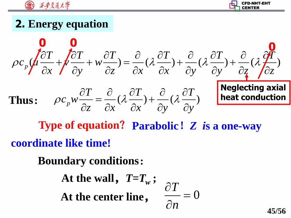
2. Energy equation
( ) ( ) ( ) ( )p
T T T T T Tc u v w
x y z x x y y z z
0 0 0
Neglecting axial heat conduction ( ) ( )p
T T Tc w
z x x y y
Thus:
Boundary conditions:
At the wall,T=Tw ;
At the center line, 0T
n
Type of equation? Parabolic!Z is a one-way
coordinate like time!

46/56
We should define an appropriate dimensionless
temperature such that the dimension of the problem
can be reduced from 3 to 2: Separating the one-way
coordinate z from the two-way coordinates x,y 。
T T
T T
b
T T
T T
w
w b
T T
T T
Then ( )b w wT T T T
( )b wT T T
z z
Defining: / , / , /( )X x D Y y D Z z DPe
p mc w DPe
4.6.2 Dimensionless governing equation
One-way coordinate!

47/56
2 2
2 2( ) 1b w
b w
m
T T X YWZ T T
W
Dependent
on Z only
Dependent on
X,Y only
0
Thus: 2 2
2 20;
m
W
X Y W
( ) 1b w
b w
T T
Z T T
d
d
At the wall 0
At center line, 0n
Dimensionless
governing eq.
Heat conduction with an inner source!

48/56
4.6.3 Analysis on the unique solution condition
Because of the homogeneous character,these also
exists an uncertainty of being magnifying by any times!
Introducing average temperature (difference):
( )w
Aw b
A
T T wdA
T TwdA
w
w bw b A
w b m
T TwdA
T TT T
T T w A
11 w
w b mA
T T wdA
A T T w
1
1 ( )mA
WdA
A W
It is the additional condition for the unique solution.
Numerical solution method is the same as that for a
circular tube.
49/56
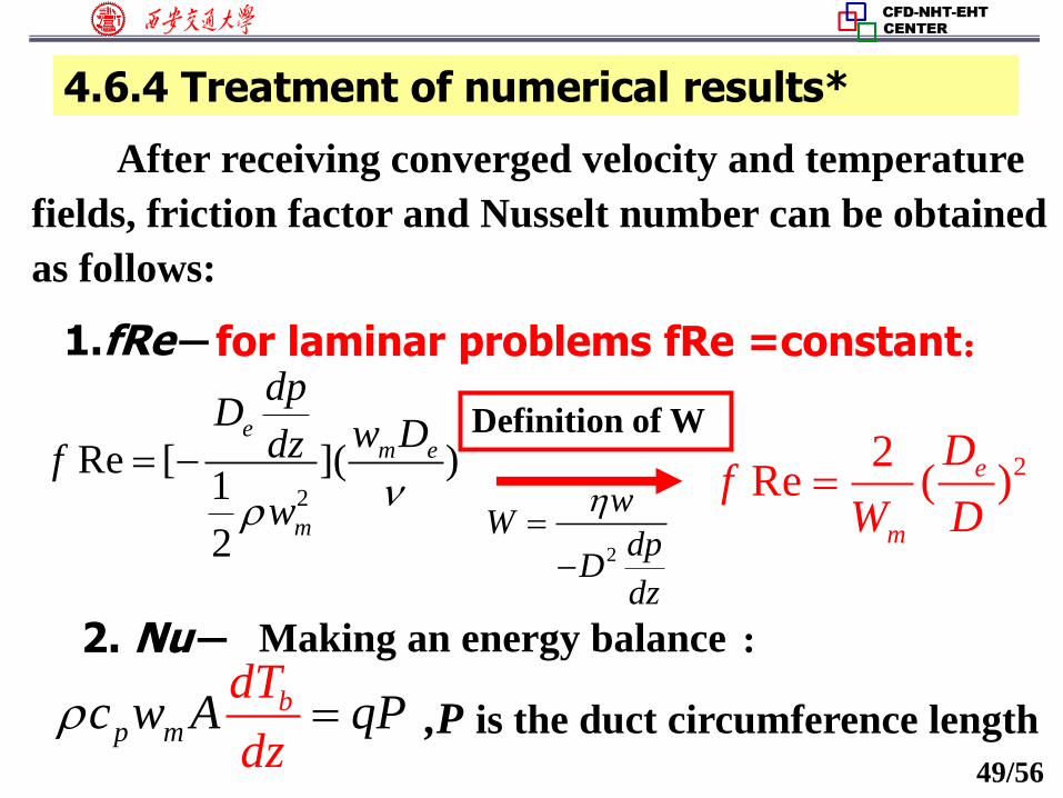
4.6.4 Treatment of numerical results*
After receiving converged velocity and temperature
fields, friction factor and Nusselt number can be obtained
as follows:
1.fRe-
2
Re [ ]( )1
2
em e
m
dpD
w Ddzf
w
Definition of W
22Re ( )e
m
Df
W D
2. Nu- Making an energy balance :
mb
p
dT
dc w A q
zP ,P is the duct circumference length
2
wW
dpD
dz
for laminar problems fRe =constant:

50/56
( ) 1b w
b w
d T T
dZ T T
i.e., ( )b b
w b
dT dTDPe T T
d dzZ
1( )
p m p m
w bb
A c w A c wq T T
P P DP
dT
dz e
mb
p
dT
dc w A q
zP
Substituting in
yields
yields: 2
( )w b
Aq T T
P D
e e
w b
hD q DNu
T T
2
1( )w b
w
e
b
T TT T
D A
P D
21( )
4
eD
D
1( )b
w b
dTT T
d DPez
4e
AD
P
p mc w DPe

53/56
Problem 4-2: As shown in Fig. 4-22, in 1-D steady heat
conduction problem, known conditions are: T1=150, Lambda=5,
S=150, Tf=25, h=15, the units in every term are consistent. Try
to determine the values of T2,T3; Prove that the solution meet
the overall conservation requirement even though only three
nodes are used.
Problem 4-4: A large plate with thickness of 0.1 m, uniform
source ;One of its wall is kept at
75 ,while the other wall is cooled by a fluid with and heat
transfer coefficient .
Adopt Practice B, divide the plate thickness into three uniform CVs,
determine the inner node temperature. Take 2nd order accuracy for the
inner node, adopt the additional source term method for the right
boundary node.
3 3S=50 10 W/m , 10 W / (m C)
25 CfT 2
50 W/m Ch
C

55/56
Problem 4-18: Shown in Fig.4-25 is a laminar fully developed heat
transfer in a duct of half circular cross. Try:
(1) Write the mathematical formulation of the heat transfer problem;
(2) Make the formulation dimensionless by introducing some
dimensionless parameters;
(3) Derive the expressions for fRe and Nu from numerical solutions,
where the characteristic length for Re and Nu is the equivalent
diameter De.