Chapter 4 PMOR

SS 2015 Production Management & Operations Research 4 - 1

Lehrstuhl für Management Science

http://www.mansci.ovgu.de

§ 4: Lot Sizing

4.1. The Economic Order Quantity (EOQ)

4.1.1 The EOQ-Formula

4.1.2 Example

4.1.3 Properties

4.1.4 Sensitivity Analysis

4.1.5 Further Remarks

4.2. The Economic Batch Quantity (EBQ)

4.3. Dynamic Lot Sizing

4.3.1. The Wagner-Whitin-Problem

4.3.2. Heuristics for dynamic lot-sizing

4.3.3. An exact approach to the dynamic lot-sizing problem




Literature

Nahmias, S. (2005), 183-202; 346-366

Krajewski, L. J.; Ritzman, L. P. (2002), 593-607; 731-796

Heizer, J.; Render, B. (2006), 473-513; 549-586

§ 4: Lot Sizing




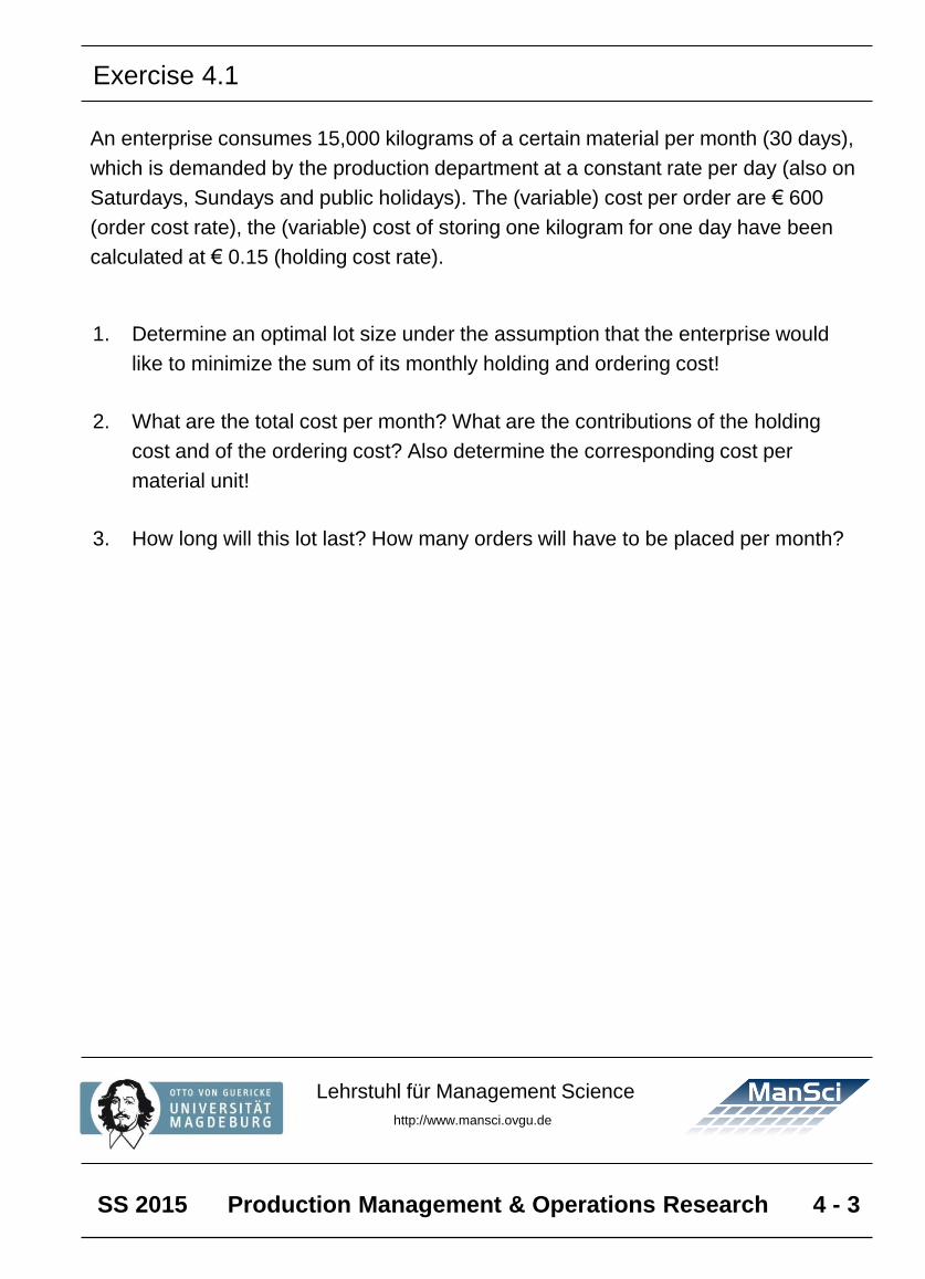
An enterprise consumes 15,000 kilograms of a certain material per month (30 days),

which is demanded by the production department at a constant rate per day (also on

Saturdays, Sundays and public holidays). The (variable) cost per order are € 600

(order cost rate), the (variable) cost of storing one kilogram for one day have been

calculated at € 0.15 (holding cost rate).

1. Determine an optimal lot size under the assumption that the enterprise would

like to minimize the sum of its monthly holding and ordering cost!

2. What are the total cost per month? What are the contributions of the holding

cost and of the ordering cost? Also determine the corresponding cost per

material unit!

3. How long will this lot last? How many orders will have to be placed per month?

Exercise 4.1




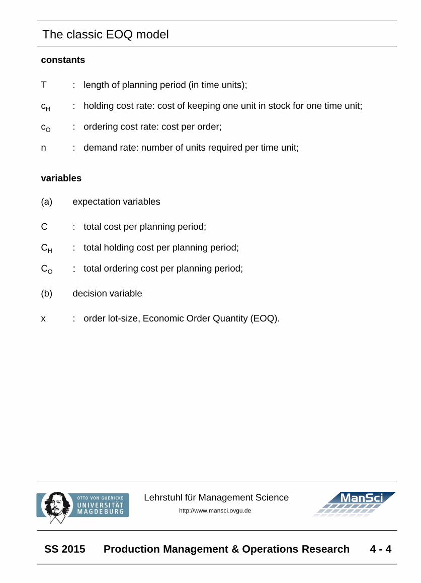
constants

T : length of planning period (in time units);

cH : holding cost rate: cost of keeping one unit in stock for one time unit;

cO : ordering cost rate: cost per order;

n : demand rate: number of units required per time unit;

variables

(a) expectation variables

C : total cost per planning period;

CH : total holding cost per planning period;

CO : total ordering cost per planning period;

(b) decision variable

x : order lot-size, Economic Order Quantity (EOQ).

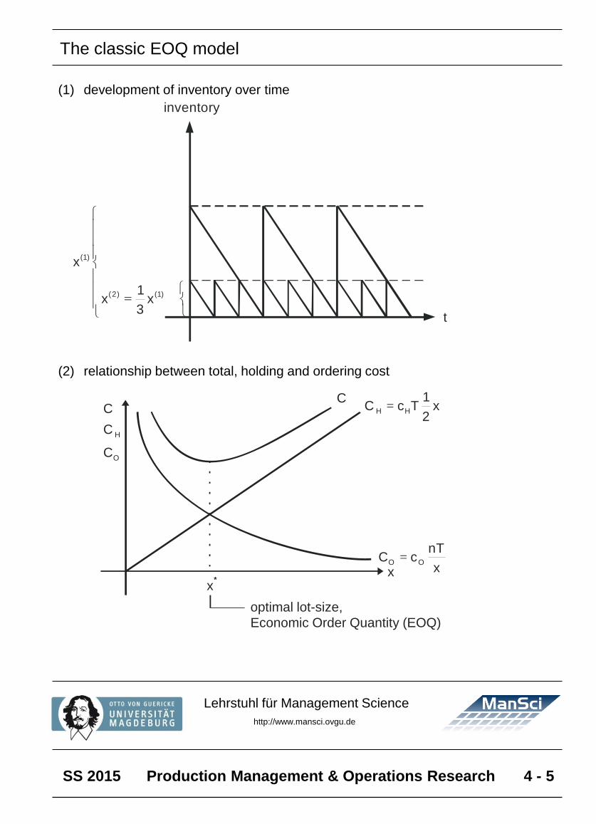
The classic EOQ model




(1) development of inventory over time

(2) relationship between total, holding and ordering cost

H

O

C

C

C

CH H

1C c T x

2=

O O

nTC c

x=

x*

x

optimal lot-size,

Economic Order Quantity (EOQ)

(1)

(2) (1)

x

1x x

3

=

t

inventory

The classic EOQ model




inc

rea

se

of

tota

l c

os

t(%

)

6.0

66

0.1

39

0.0

33

0.0

01

0.0

00

0.0

01

0.0

30

0.1

14

2.0

62

tota

l c

os

tfo

r

no

n-o

pti

ma

l

lot-

siz

e

6,7

50

.0

8,5

50

.0

8,7

75

.0

8,9

55

.0

9,0

00

.0

9,0

45

.0

9,2

25

.0

9,4

50

.0

11

,25

0.0

tota

l c

os

tfo

r

op

tim

al

lot-

siz

e

6,3

64

.0

8,5

38

.1

8,7

72

.1

8,9

54

.9

9,0

00

.0

9,0

44

.9

9,2

22

.3

9,4

39

.3

11

,02

2.7

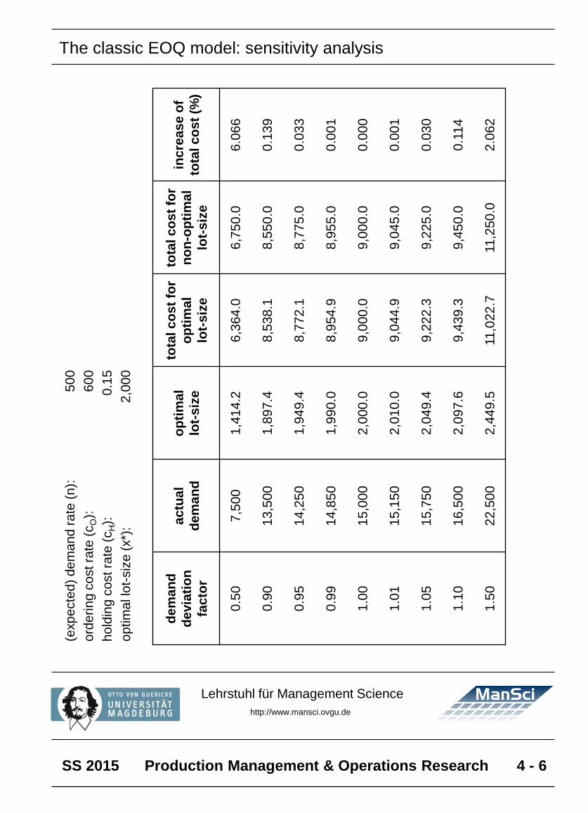
500

600

0.1

5

2,0

00

op

tim

al

lot-

siz

e

1,4

14

.2

1,8

97

.4

1,9

49

.4

1,9

90

.0

2,0

00

.0

2,0

10

.0

2,0

49

.4

2,0

97

.6

2,4

49

.5

(exp

ecte

d)

de

ma

nd

rate

(n

):

ord

erin

gco

stra

te (

cO):

hold

ing

co

stra

te (

cH):

op

tim

al lo

t-siz

e (

x*)

: ac

tua

l

de

ma

nd

7,5

00

13

,50

0

14

,25

0

14

,85

0

15

,00

0

15

,15

0

15

,75

0

16

,50

0

22

,50

0

de

ma

nd

de

via

tio

n

fac

tor

0.5

0

0.9

0

0.9

5

0.9

9

1.0

0

1.0

1

1.0

5

1.1

0

1.5

0

The classic EOQ model: sensitivity analysis




Customers demand 15,000 kilograms per month (30 days) of a certain final product

from a manufacturing company. The demand is coming in at a – more or less –

constant rate. The company produces at a constant rate of 1,500 kilograms per day

(also on Saturdays, Sundays and public holidays). The holding cost rate per product

unit (one kilogram) is 0.15 €, the (variable) set-up cost rate has been determined at

600 € per set up.

1. Determine the lot-size, which minimizes the sum of the monthly holding and set-

up costs!

2. How long is the cycle time? How many lots have to be produced in one month?

3. What are the total costs per month? What are the contributions of the holding

cost and of the set-up cost?

Exercise 4.2




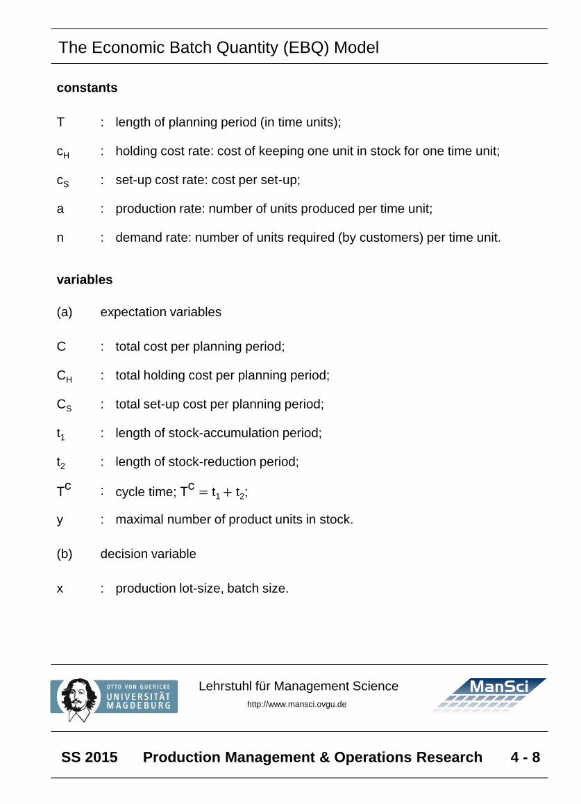
constants

T : length of planning period (in time units);

cH : holding cost rate: cost of keeping one unit in stock for one time unit;

cS : set-up cost rate: cost per set-up;

a : production rate: number of units produced per time unit;

n : demand rate: number of units required (by customers) per time unit.

variables

(a) expectation variables


CH : total holding cost per planning period;

CS : total set-up cost per planning period;

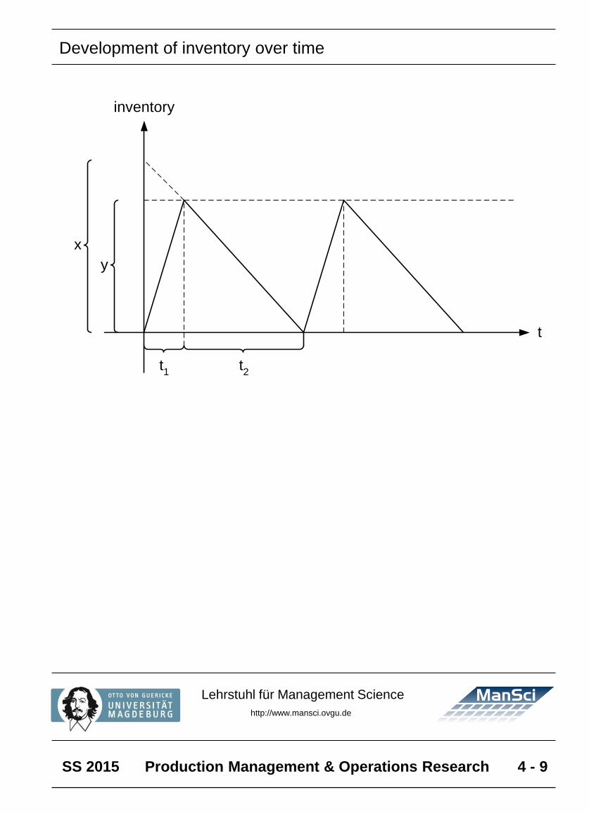
t1 : length of stock-accumulation period;

t2 : length of stock-reduction period;

Tc : cycle time; T

c = t1 + t2;

y : maximal number of product units in stock.

(b) decision variable

x : production lot-size, batch size.

The Economic Batch Quantity (EBQ) Model




x

y

t1

t2

inventory

t

Development of inventory over time




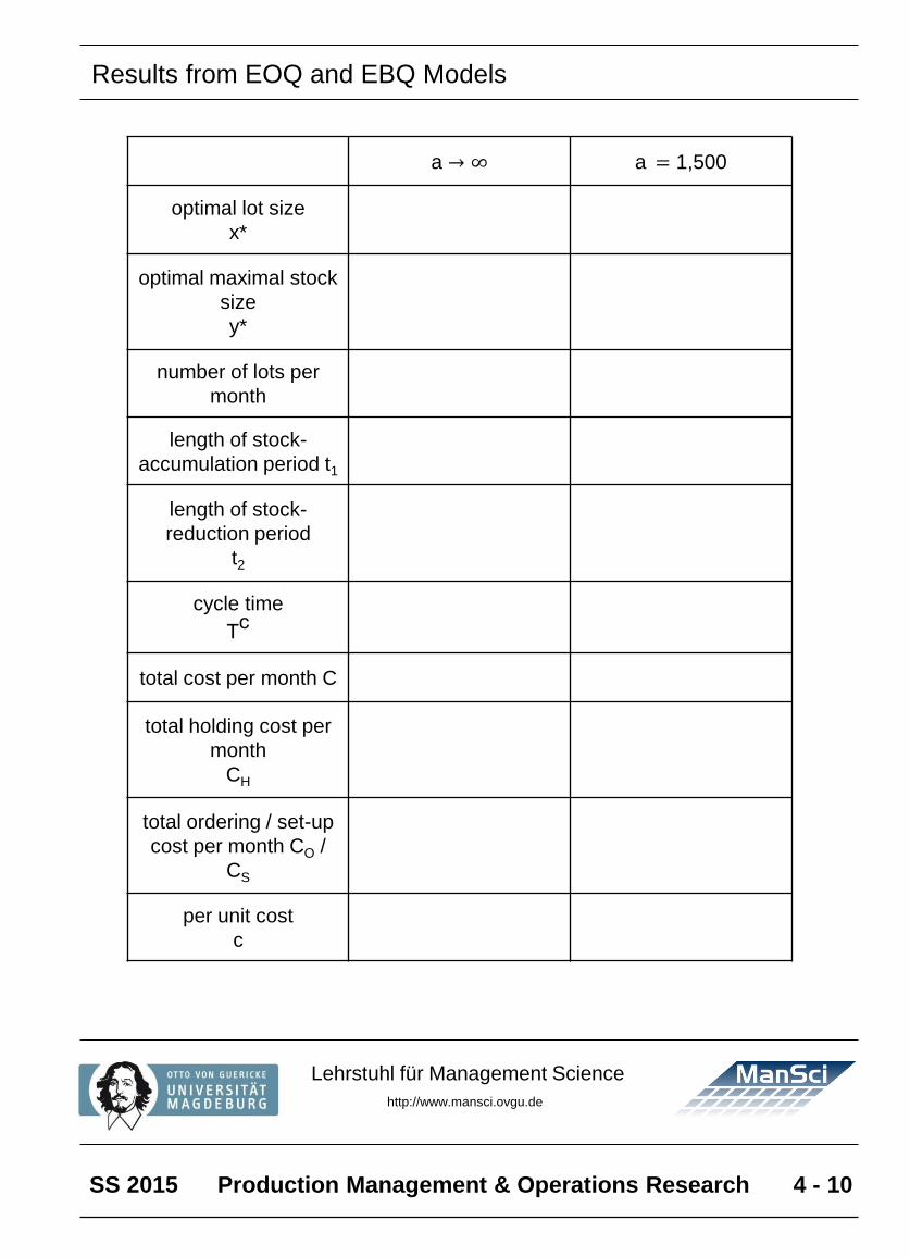
a → ∞ a = 1,500

optimal lot size

x*

optimal maximal stock

size

y*

number of lots per

month

length of stock-

accumulation period t1

length of stock-

reduction period

t2

cycle time

Tc

total cost per month C

total holding cost per

month

CH

total ordering / set-up

cost per month CO /

CS

per unit cost

c

Results from EOQ and EBQ Models




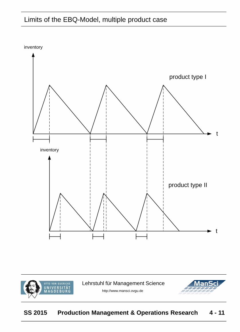
t

t

inventory

inventory

product type II

product type I

Limits of the EBQ-Model, multiple product case




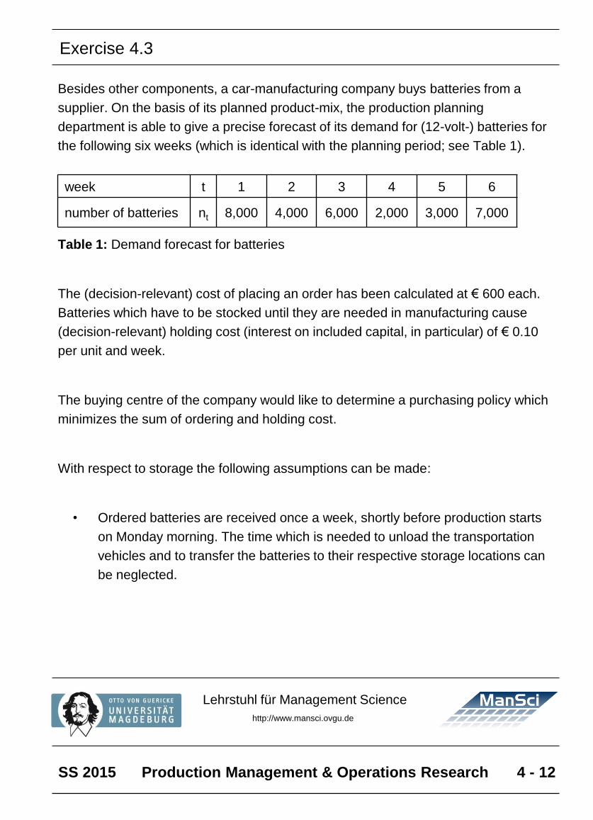
Besides other components, a car-manufacturing company buys batteries from a

supplier. On the basis of its planned product-mix, the production planning

department is able to give a precise forecast of its demand for (12-volt-) batteries for

the following six weeks (which is identical with the planning period; see Table 1).

Table 1: Demand forecast for batteries

The (decision-relevant) cost of placing an order has been calculated at € 600 each.

Batteries which have to be stocked until they are needed in manufacturing cause

(decision-relevant) holding cost (interest on included capital, in particular) of € 0.10

per unit and week.

The buying centre of the company would like to determine a purchasing policy which

minimizes the sum of ordering and holding cost.

With respect to storage the following assumptions can be made:

• Ordered batteries are received once a week, shortly before production starts

on Monday morning. The time which is needed to unload the transportation

vehicles and to transfer the batteries to their respective storage locations can

be neglected.

week t 1 2 3 4 5 6

number of batteries nt 8,000 4,000 6,000 2,000 3,000 7,000

Exercise 4.3




• Likewise, withdrawals from stock only take place once a week directly before

the start of production on Monday morning.

• There will be no batteries available for manufacturing on Monday morning of the

first week unless an order is placed. In other words: Inventory of batteries on

hand is zero.

• The planned inventory for the end of the last week is zero.

Assignments

1. Formulate a mathematical model (Wagner-Whitin-Model) from which an optimal

ordering policy can be determined!

2. By means of standard LP-software, determine an optimal solution of the

described problem and give an interpretation of the results!

3. Elaborate some of the assumptions of the Wagner-Whitin-Model which have not

been mentioned explicitly!

4. Determine an ordering policy by means of the following heuristics:

• Least-Unit-Cost Method

• Silver-Meal-Heuristic

• Part-Period-Method.

Exercise 4.3 (cont.)




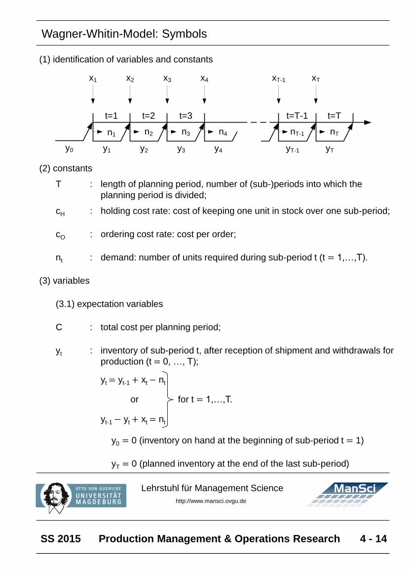
(1) identification of variables and constants

(2) constants

T : length of planning period, number of (sub-)periods into which the

planning period is divided;

cH : holding cost rate: cost of keeping one unit in stock over one sub-period;

cO : ordering cost rate: cost per order;

nt : demand: number of units required during sub-period t (t = 1,…,T).

(3) variables

(3.1) expectation variables


yt : inventory of sub-period t, after reception of shipment and withdrawals for

production (t = 0, …, T);

yt = yt-1 + xt − nt

or for t = 1,…,T.

yt-1 − yt + xt = nt

y0 = 0 (inventory on hand at the beginning of sub-period t = 1)

yT = 0 (planned inventory at the end of the last sub-period)

y2y1 y3 y4 yT-1 yT

t=1 t=2 t=3 t=T-1 t=T

n2n1 n3 n4 nT-1 nT

x2x1 x3 x4 xT-1 xT

y0

Wagner-Whitin-Model: Symbols




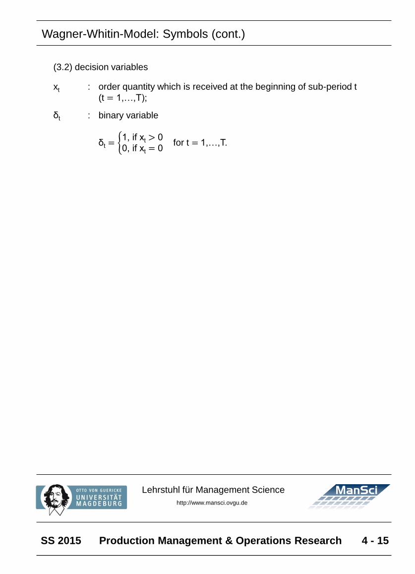
(3.2) decision variables

xt : order quantity which is received at the beginning of sub-period t

(t = 1,…,T);

δt : binary variable

δt = 1, if xt > 0

0, if xt = 0for t = 1,…,T.

Wagner-Whitin-Model: Symbols (cont.)




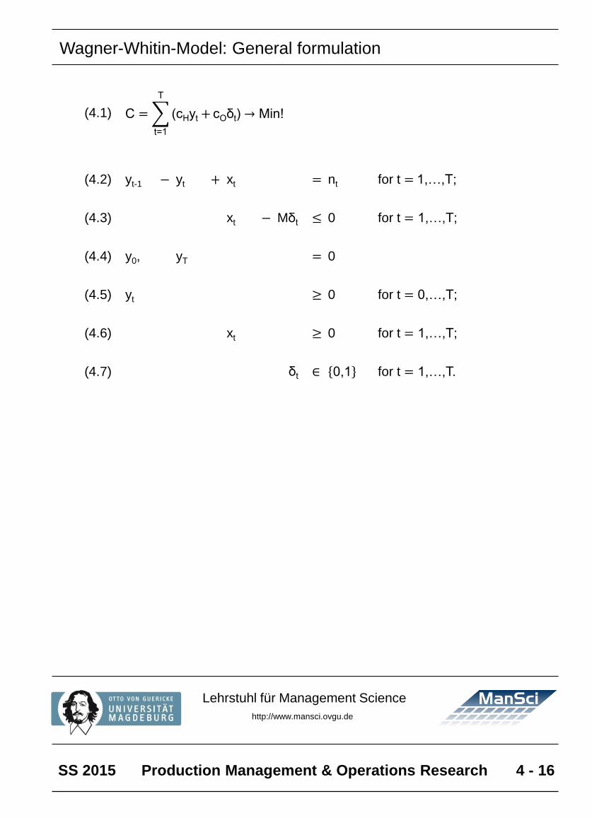
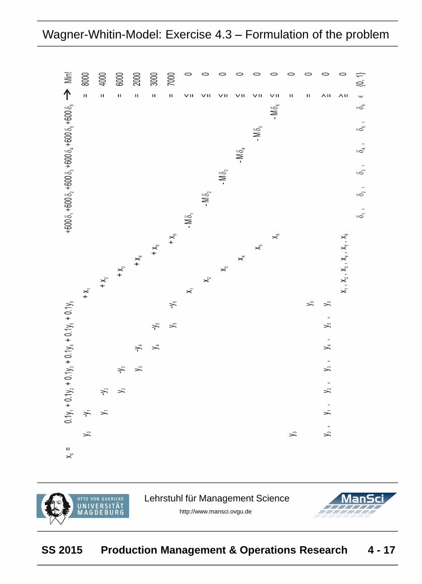
(4.1) C =

t=1

T

(cHyt + cOδt) → Min!

(4.2) yt-1 − yt + xt = nt for t = 1,…,T;

(4.3) xt − Mδt ≤ 0 for t = 1,…,T;

(4.4) y0, yT = 0

(4.5) yt ≥ 0 for t = 0,…,T;

(4.6) xt ≥ 0 for t = 1,…,T;

(4.7) δt ∈ 0,1 for t = 1,…,T.

Wagner-Whitin-Model: General formulation




Wagner-Whitin-Model: Exercise 4.3 – Formulation of the problem




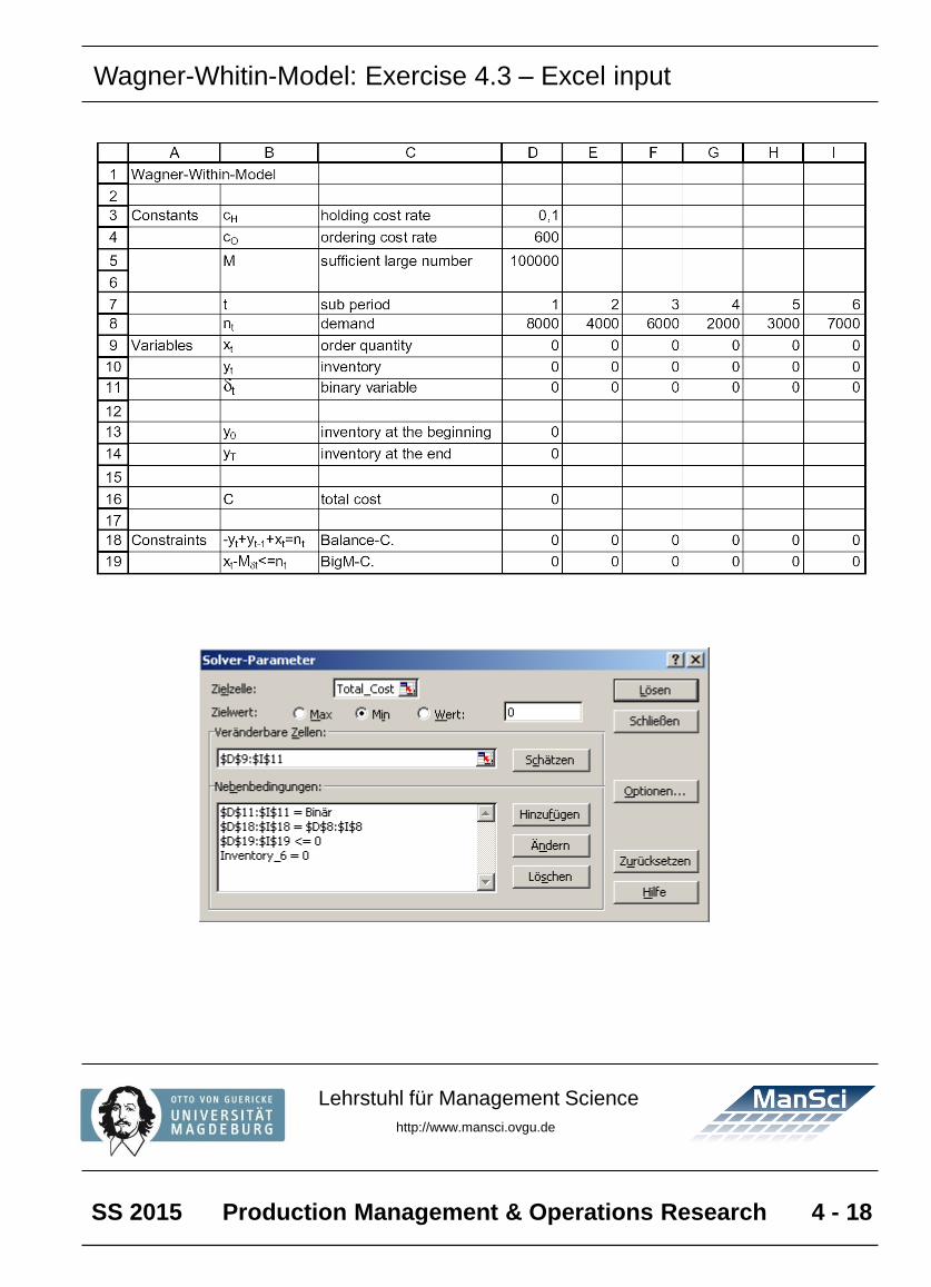
Wagner-Whitin-Model: Exercise 4.3 – Excel input




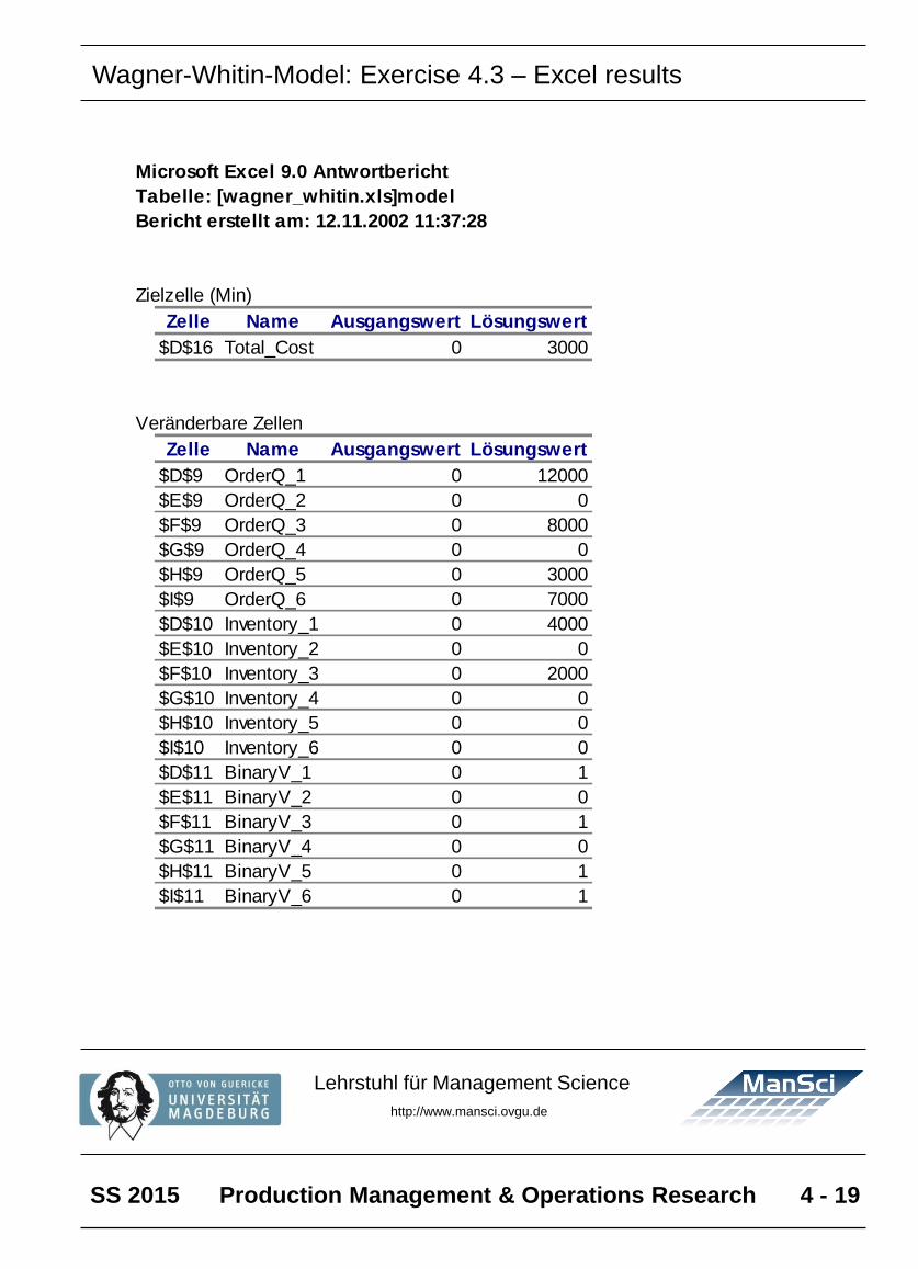
Microsoft Excel 9.0 Antwortbericht

Tabelle: [wagner_whitin.xls]model

Bericht erstellt am: 12.11.2002 11:37:28

Zielzelle (Min)

Zelle Name Ausgangswert Lösungswert

$D$16 Total_Cost 0 3000

Veränderbare Zellen

Zelle Name Ausgangswert Lösungswert

$D$9 OrderQ_1 0 12000

$E$9 OrderQ_2 0 0

$F$9 OrderQ_3 0 8000

$G$9 OrderQ_4 0 0

$H$9 OrderQ_5 0 3000

$I$9 OrderQ_6 0 7000

$D$10 Inventory_1 0 4000

$E$10 Inventory_2 0 0

$F$10 Inventory_3 0 2000

$G$10 Inventory_4 0 0

$H$10 Inventory_5 0 0

$I$10 Inventory_6 0 0

$D$11 BinaryV_1 0 1

$E$11 BinaryV_2 0 0

$F$11 BinaryV_3 0 1

$G$11 BinaryV_4 0 0

$H$11 BinaryV_5 0 1

$I$11 BinaryV_6 0 1

Wagner-Whitin-Model: Exercise 4.3 – Excel results




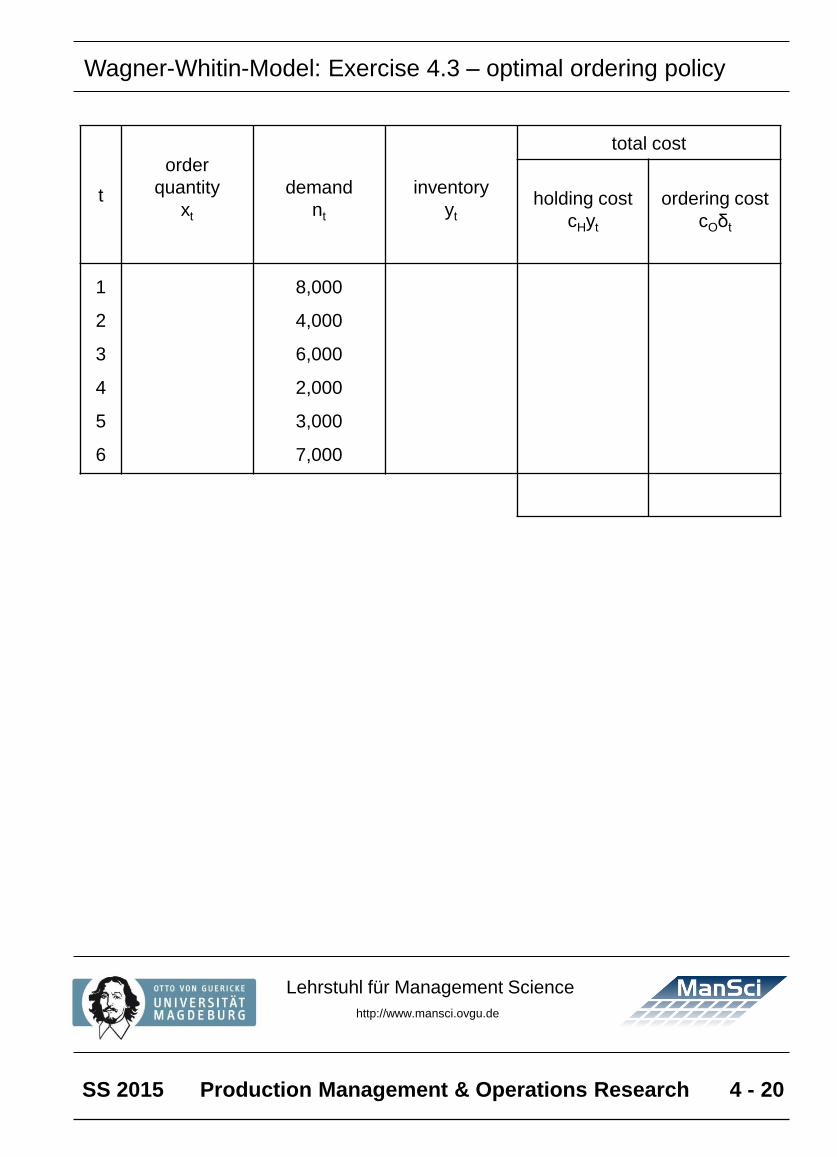
t

order

quantity

xt

demand

nt

inventory

yt

total cost

holding cost

cHyt

ordering cost

cOδt

1

2

3

4

5

6

8,000

4,000

6,000

2,000

3,000

7,000

Wagner-Whitin-Model: Exercise 4.3 – optimal ordering policy




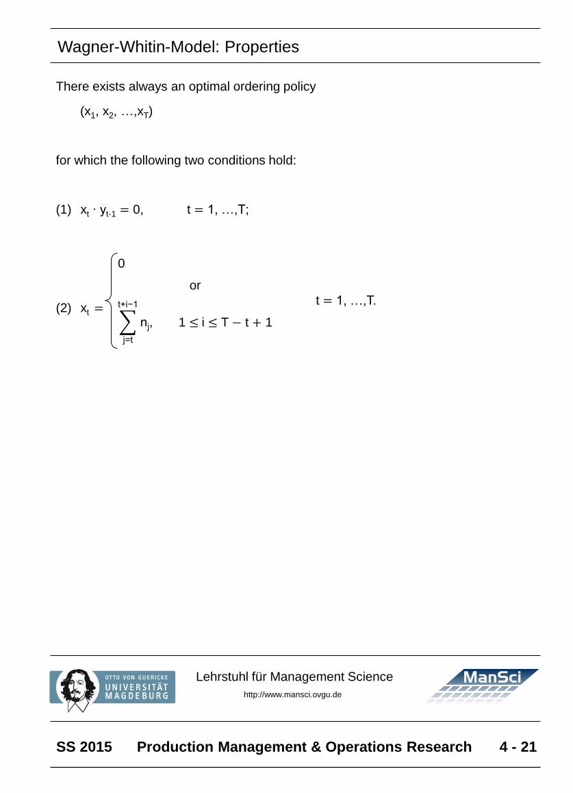
There exists always an optimal ordering policy

(x1, x2, …,xT)

for which the following two conditions hold:

(1) xt ∙ yt-1 = 0, t = 1, …,T;

(2) xt =

0

t = 1, …,T.

or

j=t

t+i−1

nj, 1 ≤ i ≤ T − t + 1

Wagner-Whitin-Model: Properties




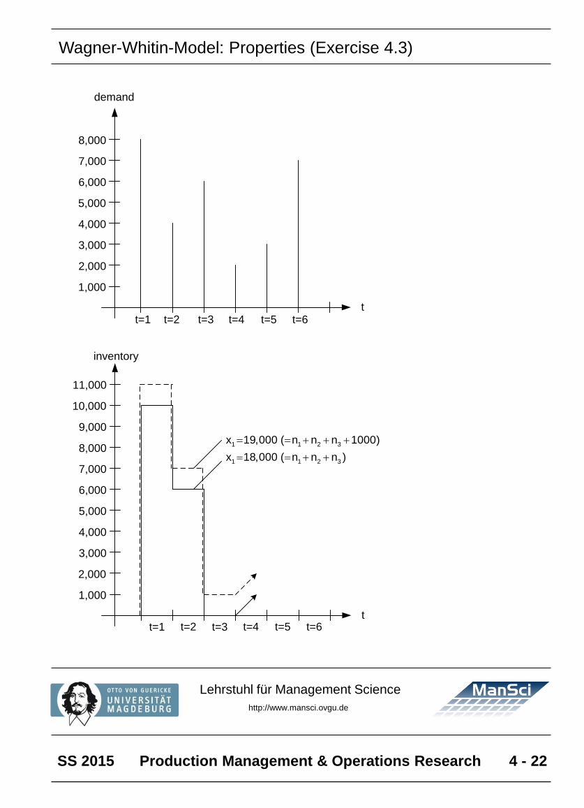
9,000

t=1 t=2 t=3 t=4 t=5 t=6t

1,000

2,000

3,000

4,000

5,000

6,000

7,000

8,000

inventory

10,000

11,000

1 1 2 3

1 1 2 3

x 19,000 ( n n n 1000)

x 18,000 ( n n n )

= =

= =

t=1 t=2 t=3 t=4 t=5 t=6t

1,000

2,000

3,000

4,000

5,000

6,000

7,000

8,000

demand

Wagner-Whitin-Model: Properties (Exercise 4.3)




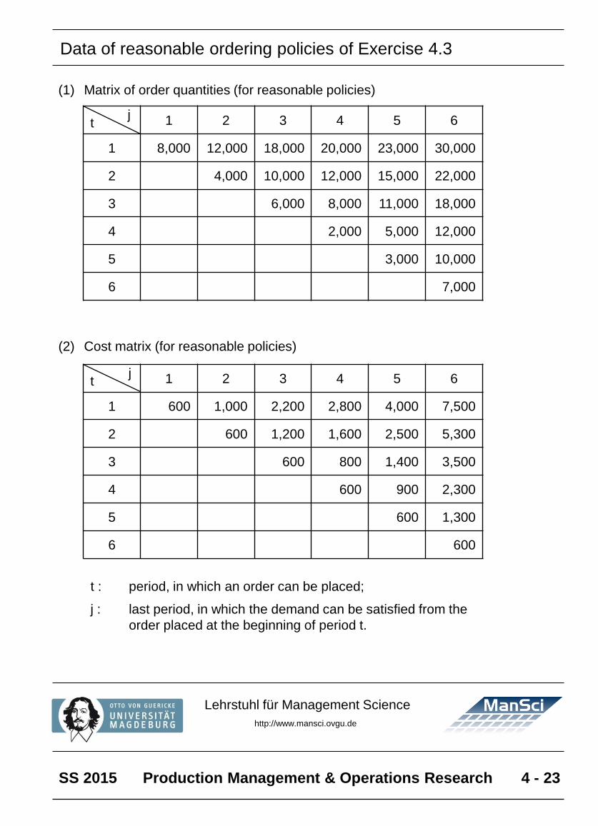
(1) Matrix of order quantities (for reasonable policies)

(2) Cost matrix (for reasonable policies)

t : period, in which an order can be placed;

j : last period, in which the demand can be satisfied from the

order placed at the beginning of period t.

t 1 2 3 4 5 6

1 8,000 12,000 18,000 20,000 23,000 30,000

2 4,000 10,000 12,000 15,000 22,000

3 6,000 8,000 11,000 18,000

4 2,000 5,000 12,000

5 3,000 10,000

6 7,000

j

t 1 2 3 4 5 6

1 600 1,000 2,200 2,800 4,000 7,500

2 600 1,200 1,600 2,500 5,300

3 600 800 1,400 3,500

4 600 900 2,300

5 600 1,300

6 600

j

Data of reasonable ordering policies of Exercise 4.3




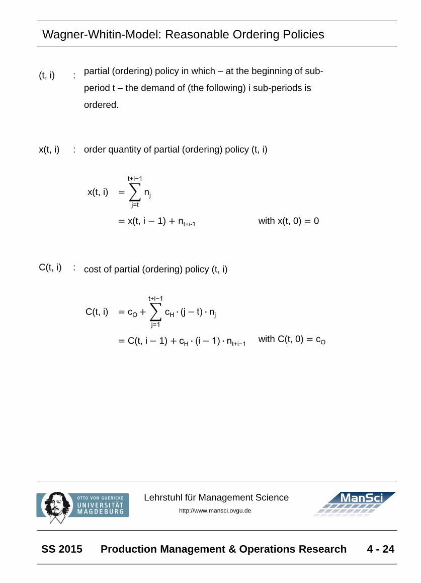
(t, i) : partial (ordering) policy in which – at the beginning of sub-

period t – the demand of (the following) i sub-periods is

ordered.

x(t, i) : order quantity of partial (ordering) policy (t, i)

x(t, i) =

j=t

t+i−1

nj

= x(t, i − 1) + nt+i-1 with x(t, 0) = 0

C(t, i) : cost of partial (ordering) policy (t, i)

C(t, i) = cO +

j=1

t+i−1

cH ∙ (j − t) ∙ nj

= C(t, i − 1) + cH ∙ (i − 1) ∙ nt+i−1with C(t, 0) = cO

Wagner-Whitin-Model: Reasonable Ordering Policies




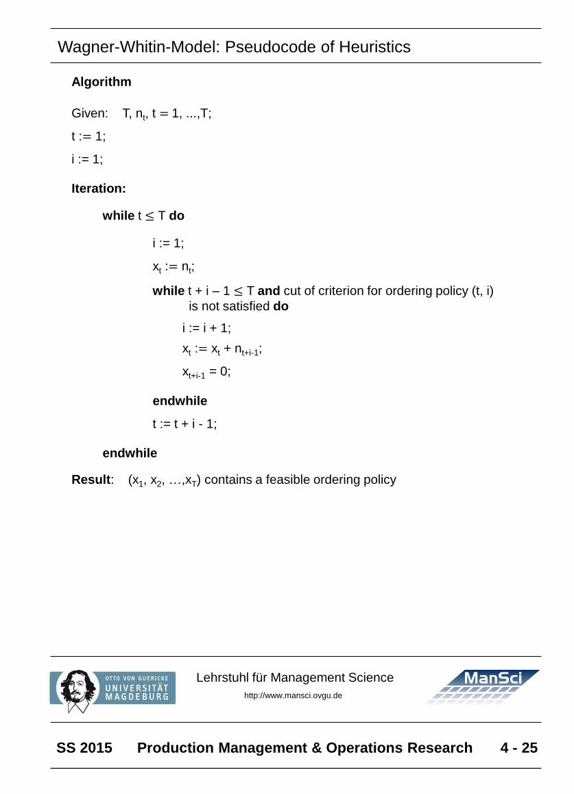
Algorithm

Given: T, nt, t = 1, ...,T;

t := 1;

i := 1;

Iteration:

while t ≤ T do

i := 1;

xt := nt;

while t + i – 1 ≤ T and cut of criterion for ordering policy (t, i)

is not satisfied do

i := i + 1;

xt := xt + nt+i-1;

xt+i-1 = 0;

endwhile

t := t + i - 1;

endwhile

Result: (x1, x2, …,xT) contains a feasible ordering policy

Wagner-Whitin-Model: Pseudocode of Heuristics




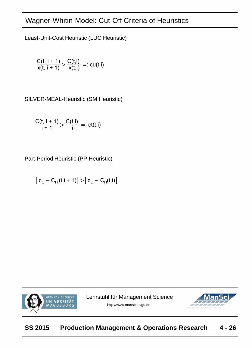
Least-Unit-Cost Heuristic (LUC Heuristic)

C(t, i + 1)x(t, i + 1)

>C(t,i)x(t,i)

=: cu(t,i)

SILVER-MEAL-Heuristic (SM Heuristic)

C(t, i + 1)i + 1

>C(t,i)

i=: ct(t,i)

Part-Period Heuristic (PP Heuristic)

│cO − CH (t,i + 1)│>│cO − CH(t,i)│

Wagner-Whitin-Model: Cut-Off Criteria of Heuristics




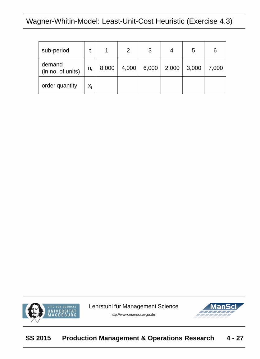
sub-period t 1 2 3 4 5 6

demand

(in no. of units)nt 8,000 4,000 6,000 2,000 3,000 7,000

order quantity xt

Wagner-Whitin-Model: Least-Unit-Cost Heuristic (Exercise 4.3)





demand

(in no. of units)nt 8,000 4,000 6,000 2,000 3,000 7,000

order quantity xt

Wagner-Whitin-Model: SILVER-MEAL-Heuristic (Exercise 4.3)





demand

(in no. of units)nt 8,000 4,000 6,000 2,000 3,000 7,000

order quantity xt

Wagner-Whitin-Model: Part-Period-Heuristic (Exercise 4.3)




tota

l

co

st

ord

erin

g

co

st

hold

ing

co

st

ord

ering

polic

y

x6

x5

x4

x3

x2

x1

op

tim

iza

tion

mo

de

l

lea

st-

unit-c

ost-

me

thod

SIL

VE

R-M

EA

L-h

eu

ristic

pa

rt-p

erio

d-m

eth

od

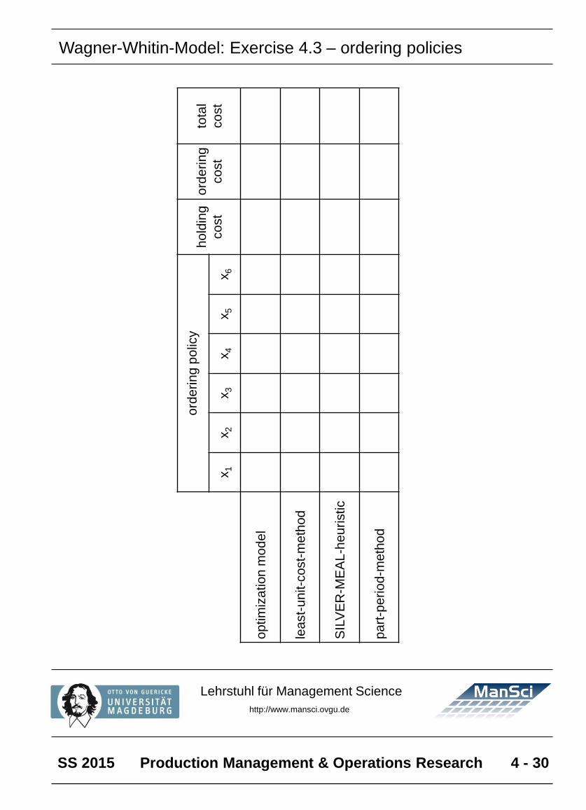
Wagner-Whitin-Model: Exercise 4.3 – ordering policies

Documents

Chapter 4 PMOR