Chapter 5 Cycles and Circuits

Chapter 5

Cycles and Circuits

Section 5.1 Eulerian Graphs

Probably the oldest and best known of all problems in graph theory centers on thebridges over the river Pregel in the city of Ko

. .nigsberg (presently called Kaliningrad in

Russia). The legend says that the inhabitants of Ko. .nigsberg amused themselves by

trying to determine a route across each of the bridges between the two islands (A and B inFigure 5.1.1), both river banks (C and D of Figure 5.1.1) and back to their starting pointusing each bridge exactly one time. After many attempts, they all came to believe thatsuch a route was not possible. In 1736, Leonhard Euler [15] published what is believedto be the first paper on graph theory, in which he investigated the Ko

. .nigsberg bridge

problem in mathematical terms.

A B

D

C

Figure 5.1.1. The bridges on the river Pregel.

The solution to the bridge problem hinges on the degrees of the vertices in the graphmodel for the bridges and land masses (see Figure 5.1.2). The problem seeks a circuitthat contains each edge. In honor of Euler, we say a graph (or multigraph) is eulerian ifit has a circuit containing all the edges of the graph. The circuit itself is called aneulerian circuit. A trail containing every edge of the graph is called an eulerian trail.

Several characterizations have been developed for eulerian graphs. Euler hasfrequently been credited with the complete equivalence of statements 1 and 2 in Theorem5.1.1; however, he actually established only half of it ( 1 → 2 ). Hierholzer [33]established the converse. The result below is a blend of the work of Euler [15],Hierholzer [33] and Veblen [46].

2 Chapter 5: Cycles and Circuits

A B

C

D

Figure 5.1.2. The multigraph of the bridges.

Theorem 5.1.1 The following statements are equivalent for a connected graph G:

1. The graph G contains an eulerian circuit.

2. Each vertex of G has even degree.

3. The edge set of G can be partitioned into cycles.

Proof. To see that (1) implies (2), let v be a vertex of G. If C is an eulerian circuit in G,then each edge of G entering v must be matched by another edge leaving v. Thus, thedegree of any vertex must be even.

To establish that (2) implies (3), we use induction on the number of cycles in thegraph. Clearly, the result holds if there are no cycles or there is one cycle in G. Now,assume the result holds if there are fewer than k cycles in G and suppose that G is aconnected graph with all vertices having even degree and containing exactly k cycles.Delete the edges of one cycle C * of G. Each component of the remaining graph clearlyhas the property that all vertices have even degree. Further, each component has fewerthan k cycles, and, thus, by the induction hypothesis, their edge sets can be partitionedinto cycles. The edge set of G can then be partitioned in a similar manner and along withC * we obtain the desired partition of E(G).

Finally, to see that (3) implies (1), assume that the edge set of G can be partitionedinto cycles and suppose there are m such cycles. We use induction to establish that forany k ( 1 ≤ k ≤ m), there is a circuit in G which contains each edge of k of the cycles andno other edge of G. The statement is clear if k = 1, since a single cycle suffices. Thus,we assume there is a circuit C which contains k of the cycles (k < m) and no other edgesof G. Since G is connected, at least one of the other cycles must contain a vertex of C.

Chapter 5: Cycles and Circuits 3

Let C 1 be the circuit obtained by traversing that cycle, beginning at some commonvertex v (and, hence, returning there), and then following C. Then clearly, C 1 containsthe edges of k + 1 cycles and no other edges; hence, the result follows by induction.

Since every graph contains an even number of vertices of odd degree, the followingcorollary is easily obtained.

Corollary 5.1.1 A connected graph G contains an eulerian trail if, and only if, at mosttwo vertices of G have odd degree.

We can, however, extend Corollary 5.1.1 a little further. The proof is left to theexercises.

Corollary 5.1.2 Let G = (V , E) be a connected graph with 2k (k > 0 ) vertices ofodd degree. Then E can be partitioned into exactly k open trails.

These ideas can certainly be extended to directed graphs. The literature on thissubject contains a wide variety of terms for such digraphs. We shall simply call themeulerian digraphs. The following result is analogous to Theorem 5.1.1. Its proof is alsoleft to the exercises.

Theorem 5.1.2 The following statements are equivalent for a connected digraphD = (V , E):

1. The digraph D has a directed eulerian circuit.

2. For each vertex v ∈ V, id v = od v.

3. The arc set E can be partitioned into directed cycles.

Next, we wish to consider algorithms designed to produce eulerian circuits. Perhapsthe oldest such algorithm is from Fleury [22]. Fleury’s approach is to construct a trail Cthat will grow to be the desired eulerian circuit, constantly expanding the number ofedges being used in C, while avoiding bridges in the graph formed by the edges not yetincluded in C. A bridge is selected only when no other choice remains. The postponingof the use of bridges is really the critical feature of this algorithm, and its purpose is toavoid becoming trapped in some component of G − C.

Algorithm 5.1.1 Fleury’s Algorithm.


Input: A connected (p , q) graph G = (V , E).Output: An eulerian circuit C of G.Method: Expand a trail C i while avoiding bridges in G − C i , until

no other choice remains.

1. Choose any v 0 ∈ V and let C 0 = v 0 and i ← 0.

2. Suppose that the trail C i = v 0 , e 1 , v 1 , . . . , e i , v i has already been chosen:

a. At v i , choose any edge e i + 1 that is not on C i and that is not a bridge of thegraph G i = G − E(C i ), unless there is no other choice.

b. Define C i + 1 = C i , e i + 1, v i + 1.

c. Let i ← i + 1.

3. If i = ⎪E⎪then halt since C = C i is the desired circuit;else go to 2.

Theorem 5.1.3 If G is eulerian, then any circuit constructed by Fleury’s algorithm iseulerian.

Proof. Let G be an eulerian graph. Let C p = v 0 , e 1 , . . . , e p , v p be the trailconstructed by Fleury’s algorithm. Then clearly, the final vertex v p must have degree 0in the graph G p , and hence v p = v 0, and C p is a circuit.

Now, to see that C p is the desired circuit, suppose instead that C p is not an euleriancircuit of G. Thus, there must be edges of G not on C p . Let S be the set of vertices ofpositive degree in G p . Hence, S ∩ V(C p ) is nonempty since G is connected andv p ∈ S

_= V − S. Let i be the largest integer such that v i ∈ S ∩ C p but v i + 1 ∈ S

_.

Since C p ends in S_, it follows that i < p. From the definition of S

_, each edge of G i that

joins S and S_

is on C p; thus, the edge e i + 1 is the only edge from S to S_

in the graph G i .But then e i + 1 is a bridge in G i .

Suppose that e is any other edge of G i that is incident to v i . Then from step 2 of thealgorithm, it follows that e must also be a bridge of G i (and, hence, of the graph H i ,induced by S in G i). Since H i ⊆ H p (the graph induced by S in G p), it follows that e isalso a bridge in H p . Further, since e i + 1 is a bridge of G i and v i is the last vertex on C pthat is also in S, we see that H i = H p and that deg H p

v = deg G pv for every vertex v of

H p . Thus, every vertex in H p has even degree. But we know from exercise 15 inChapter 2 that this implies that H p contains no bridges, a contradiction.


Can you determine the complexity of Fleury’s algorithm?

Hierholzer [33] developed an algorithm that produces circuits in a graph G which arepairwise edge disjoint. When these circuits are put together properly, they form aneulerian circuit of G. This patching together of circuits hinges of course, on the circuitshaving a common vertex, and this fact follows from the connectivity of the graph. Onceone circuit is formed, if all edges have not been used, then there must be one edge that isincident to a vertex of the circuit, and we use this edge to begin the next circuit. Thesecircuits then share a common vertex.

Algorithm 5.1.2 Hierholzer’s Algorithm.Input: A connected graph G = (V , E), each of whose vertices has even degree.Output: An eulerian circuit C of G.Method: Patching together of circuits.

1. Choose v ∈ V. Produce a circuit C 0 beginning with v by traversing at each step,any edge not yet included in the circuit. Set i = 0.

2. If E(C i ) = E(G);then halt since C = C i is an eulerian circuit;else choose a vertex v i on C i that is incident to an edge not on C i . Nowbuild a circuit C i

* beginning with v i in the graph G − E(C i ). (Hence, C i*

also contains v i .)

3. Build a circuit C i + 1 containing the edges of C i and C i* by starting at v i − 1,

traversing C i until reaching v i , then traversing C i* completely (hence, finishing at

v i) and then completing the traversal of C i . Now set i ← i + 1 and go to 2.

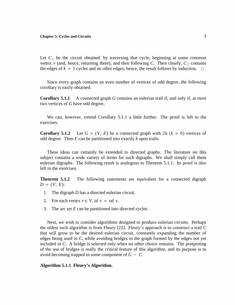
Tucker [45] developed an algorithm that is essentially a combination of the methodsof Fleury and Hierholzer. In order to present his algorithm, we need another idea. Ife 1 = vw and e 2 = vx are two edges of G, then the splitting away of e 1 and e 2 results ina new graph H obtained by deleting e 1 and e 2 from G and adding a new vertex z adjacentto w and x (see Figure 5.1.3). Note that G can be recovered from H by identifying thevertices z and v, that is, by replacing z and v with one new vertex adjacent to all theneighbors of z and v. It is clear that H is eulerian if, and only if, G is eulerian and{ e 1 , e 2 } does not form a cut set. It is also not hard to prove that H is connected if, andonly if, G is connected and { e 1, e 2 } does not form a cut set (see exercise 6 in Chapter5). We now present Tucker’s algorithm. Repetition of the splitting away process isintended to produce the cycle partition of E promised in Theorem 5.1.1.


w x

v

w x

z

v==>

Figure 5.1.3. Splitting away of e 1 and e 2.

Algorithm 5.1.3 Tucker’s Algorithm.Input: An eulerian graph G = (V , E).Output: An eulerian circuit C of G.Method: Split away the edges to form the desired cycle partition and then

form the circuit by reassembling the cycles in a controlled manner.

1. Split away pairs of edges of G until there are only vertices of degree 2 remaining.Call the graph obtained in this manner G 1. Set i ← 1 and let c i be the number ofcomponents of G i .

2. If c i = 1,then halt with C = G i;else find two components T and T * of G i with the vertex v i in common.Form a circuit C i + 1, starting at v i and traversing T and T * , ending again atv i (as discussed earlier).

3. Define G i + 1 = G i − {T , T *} ∪ C i + 1. (Here, we consider the circuit C i + 1 asbeing a component of G i + 1.) Set T = C i + 1, i ← i + 1, let c i be the number ofcomponents of G i and go to 2.

We conclude this section with the famous problem, introduced by Kwan [34] in 1960,called the Chinese postman problem. The problem is that the postman must traverse hismail route each day, traveling along each road and eventually returning to the post office,his starting point. Certainly, the postman desires a route that minimizes the total distancehe travels.

Clearly, we can use a graph to model the mail route he must eventually cover. Asolution is provided by a closed walk of minimum length that uses each edge at leastonce in the graph modeling the entire mail route.


It is a simple observation that if the (p , q) graph G models the postman’s route, thencertainly the distance the postman must travel is at least q. It is also easy to see that if thegraph under consideration is a tree, then each edge must be used twice. Certainly, there isno need to use any edge three times. Hence, for the distance d in the Chinese postmanproblem, q ≤ d ≤ 2q. It is further clear that if the graph under consideration is aneulerian graph, then the Chinese postman problem can be solved by any of our previouseulerian algorithms. Goodman and Hedetniemi [26] noticed that the problem of findingthe postman’s walk is equivalent to the problem of determining the minimum number ofedges that must be duplicated in order to produce an eulerian multigraph. One way tosolve this problem is to consider all possible pairs of vertices of odd degree and pair themaccording to the minimum distances between them. Insert these edges to form the desiredeulerian multigraph. We can now apply any of our algorithms for finding euleriancircuits to complete the task. However, in general this is not an efficient algorithm.

Edmonds and Johnson [13] provided a good algorithm for solving this problem,under the generalized condition that the edge distances were w(e) ≥ 0. However, theirsolution is beyond the scope of this text.

Section 5.2 Adjacency Conditions for Hamiltonian Graphs

In the previous section we tried to determine a tour of a graph that would use eachedge once and only once. It seems natural to vary this question and try to visit eachvertex once and only once. In fact, a cycle (path) that contains every vertex of a graph iscalled a hamiltonian cycle (path).

This terminology is used in honor of Sir William Rowan Hamilton, who, in 1865,described an idea for a game in a letter to a friend. This game, called the icosian game,consisted of a wooden dodecahedron (see Figure 5.2.1) with pegs inserted at each of thetwenty vertices. These pegs supposedly represented the twenty most important cities ofthe time. The object of the game was to mark a route (following the edges of thedodecahedron) passing through each of the cities only once and finally returning to theinitial city. Hamilton sold the idea for the game. (I think his profit was the only onemade on this game!)

From this unusual beginning has sprung a stream of interesting work concerningspanning cycles and paths in graphs. We cannot even begin to completely survey theextensive literature on this subject. Instead, we wish to hit some of the highlights andshow some of the diverse approaches taken in what has become a very interesting andimportant subject.


Figure 5.2.1. The graph of the dodecahedron.

Since the idea of a hamiltonian cycle "sounds" analogous to that of an euleriancircuit, one might expect that we will be able to establish some sort of correspondingtheory. This, however, is definitely not the case. In fact, the hamiltonian problem isNP-complete (see [24]), and no practical characterization for hamiltonian graphs hasbeen found. Hence, we shall not study any general algorithms for directly finding suchcycles. However, there has still been a considerable amount of information discoveredabout hamiltonian graphs.

Perhaps the theorem that stirred the most subsequent work is that of Ore [41]. Itstems from the idea that if a sufficient number of edges are present in the graph, then ahamiltonian cycle will exist. To ensure a sufficient number of edges, we try to keep thedegree sum of nonadjacent pairs of vertices at a fairly high level. We can see the effectthat controlling degree sums provides when we consider a vertex x of "low" degree.Since x has many nonadjacencies in the graph, the degrees of all these vertices are thenforced to be "high," to ensure that the degree sum remains sufficiently large. Thus, thegraph has many vertices of high degree, and so, one hopes it contains enough structure toensure that it is hamiltonian.

Theorem 5.2.1 If G is a graph of order p ≥ 3 such that for all pairs of distinctnonadjacent vertices x and y, deg x + deg y ≥ p, then G is hamiltonian.

Proof. Suppose the result is not true. Then there exists a maximal nonhamiltoniangraph G of order p ≥ 3 that satisfies the conditions of the theorem. That is, G isnonhamiltonian, but for any pair of nonadjacent vertices x and y in G, the graph G + xy


is hamiltonian. Since p ≥ 3, the graph G is not complete.

Now, consider H = G + xy. The graph H is hamiltonian and, in fact, everyhamiltonian cycle in H must use the edge from x to y. Thus, there is an x − yhamiltonian path P: x = v 1 , v 2 , . . . , v p = y in G. Now, observe that if v i ∈ N(x),then v i − 1 ∈/ N(y), or else (see Figure 5.2.2)

v 1 , v i , v i + 1 , . . . , v p , v i − 1 , v i − 2 , . . . , v 1

would be a hamiltonian cycle in G. Hence, for each vertex adjacent to x , there is a vertexof V − { y } not adjacent to y. But then, we see that deg y ≤ (p − 1 ) − deg x. Thatis, deg x + deg y ≤ p − 1, a contradiction.

... ...v 1 v pv i − 1 v i

Figure 5.2.2. The path P and possible adjacencies.

We now state an immediate corollary of Ore’s theorem that actually preceded it. Thisresult is originally from Dirac [11]. A more elegant proof that inspired Ore’s work wasprovided independently by Newman [40].

Corollary 5.2.1 If G is a graph of order p ≥ 3 such that δ(G) ≥2p_ _, then G is

hamiltonian.

Following Ore’s theorem, a stream of further generalizations were introduced. Thisline of investigation culminated in the following work of Bondy and Chva ́ tal [4]. Thenext result stems from their observation that Ore’s proof does not need or use the fullpower of the statement that each nonadjacent pair satisfies the degree sum condition.

Theorem 5.2.2 Let x and y be distinct nonadjacent vertices of a graph G of order psuch that deg x + deg y ≥ p. Then G + xy is hamiltonian if, and only if, G ishamiltonian.

Proof. If G is hamiltonian, then clearly G + xy is hamiltonian. Conversely, if G + xyis hamiltonian but G is not, then we proceed exactly as in Ore’s theorem to produce acontradiction to the degree sum condition.


The last result inspired the following definition. The closure of a graph G, denotedCL(G), is that graph obtained from G by recursively joining pairs of nonadjacent verticeswhose degree sum is at least p until no such pair remains. The first thing we must verifyis that this definition is well defined; that is, since no order of operations is specified, wemust verify that we always obtain the same graph, no matter what order we use to insertthese edges.

Theorem 5.2.3 If G 1 and G 2 are two graphs obtained by recursively joining pairs ofnonadjacent vertices whose degree sum is at least p until no such pair remains, thenG 1 = G 2; that is, CL(G) is well defined.

Proof. Denote by e 1 , e 2 , . . . , e i and f 1 , f 2 , . . . , f j the sequences of edgesinserted in G to form G 1 and G 2, respectively. We wish to show that each e m is in G 2and that each f n is in G 1.

Let e k = uv be the first edge in the sequence e 1 , . . . , e i that is not in G 2.Consider the graph H = G + { e 1 , . . . , e k − 1 }. Then, from the definition of G 1 itfollows that

deg H u + deg H v ≥ p.

Also, by our choice of e k , H is a subgraph of G 2. Thus,

deg G 2u + deg G 2

v ≥ p.

But this is a contradiction since u and v are nonadjacent in G 2. Similarly, each f n is inG 1 and, hence, G 1 = G 2 and the closure is well defined.

Example 5.2.1. We illustrate the construction of the closure of the graph picturedbelow.

==>


==>==>

Using Theorem 5.2.2, we see that the next result is immediate.

Theorem 5.2.4 A graph G is hamiltonian if, and only if, CL(G) is hamiltonian.

If CL(G) = K p , then it is immediate that CL(G) is hamiltonian and, hence, that G ishamiltonian. This observation offers another proof of Ore’s theorem and of Dirac’stheorem.

In [4], a O(V 3 ) algorithm for finding a hamiltonian cycle in a graph satisfying thedegree sum condition deg x + deg y ≥ ⎪V(G)⎪for all nonadjacent pairs of vertices x , y(call such graphs Ore-type) using the closure was provided. Recently, Albertson hasprovided a O(V 2 ) algorithm. His approach is based on two observations takenessentially from Ore’s proof technique.

Observation 1. In any Ore-type graph G, the vertices of any maximal path can bepermuted to form a cycle C.

Observation 2. In any Ore-type graph G, if x ∈/ V(C), then there is a path that containsx and all the vertices of C.

The proofs of these observations are left to the exercises. We now presentAlbertson’s algorithm [1].

Algorithm 5.2.1 Albertson’s Algorithm.Input: An Ore-type graph G.Output: A hamiltonian cycle in G.Method: Use of observations 1 and 2.

1. Create a maximal path P: u , . . . , x k , . . . , v.

2. Repeat while ⎪V(C)⎪ ≠ ⎪V(G)⎪.If u is adjacent to v,


then set C: u , . . . , v , u;else find a k such that u is adjacent to x k + 1 and v is adjacent to x k . SetC: u , x k + 1 , x k + 2 , . . . , v , x k , x k − 1 , . . . , x , u.

3. Find x ∈ V(G − C), and create P * , a path containing x and allof C. Set P equal to a maximal path containing P * .

4. endwhile

Next, we consider an alternate approach to ensuring a sufficient number of edges thatare properly distributed to guarantee that a graph is hamiltonian. Recently, the idea ofbounding the cardinality of the neighborhoods of nonadjacent vertices has been used todetermine when many graph properties are present. In [18], this idea was introduced andused to determine a sufficient condition for a graph to be hamiltonian. If G ≠ K p , noconnectivity condition can be forced by bounding the cardinality of neighborhood unionsof nonadjacent vertices. (That is, once we have avoided the pathological case in whichthe neighborhood condition is satisfied vacuously, then no connectivity condition can beforced by the neighborhood condition.) For example, consider the graph K r ∪ K r .Thus, we must assume some minimal connectivity condition.

Theorem 5.2.5 If G is a 2-connected graph such that for every pair of nonadjacentvertices x and y,

⎪N(x) ∪ N(y)⎪ ≥3

2p − 1_ ______,

then G is hamiltonian.

Can you find an example of a graph G which Theorem 5.2.5 shows is hamiltonian,but for which CL(G) = G?

One can consider Dirac’s theorem as providing a bound on the cardinality of theneighborhood of a single vertex, and the last result provides a bound on the cardinality ofthe neighborhood of a pair of nonadjacent vertices. In [18] it was conjectured that evenhigher connectivity conditions would allow expansion of the set of nonadjacent verticesto those with more than two vertices. Fraisse [23] verified that this conjecture was indeedtrue. We consider N(S) to be the set of neighbors of the vertices in the set S. Forconvenience, we define [x , y] to mean the segment of a path or cycle, following someorientation, from the vertex x to the vertex y (including both x and y). If we do not wishto include an end vertex we will use the notation (x , y), or a mixture of the two notationswhere appropriate.


Theorem 5.2.6 Let G be a k-connected graph of order n ≥ 3. Suppose there existssome t ≤ k such that for every set S of t mutually nonadjacent vertices,

⎪N(S)⎪ >t + 1

t(n − 1 )_ ________; then G is hamiltonian.

Proof. Suppose G is not hamiltonian and let C be a cycle of maximum length, say m, inG. Let x 0 be a vertex of G off C and fix the following ordering of C: v 1 , v 2 , . . . , v m .Using Menger’s theorem (see exercise 14 in Chapter 2), we find that there exist t pathsfrom x 0 to C that are disjoint except at x 0. Let { w 1 , w 2 , . . . , w t } denote the endvertices of these paths on C and, further, assume they occur in this order according to ourordering of C. Also, denote by x i the successor of w i with respect to this ordering alongC and let X = { x i ⎪ 0 ≤ i ≤ t }. It is clear that X is a set of t + 1 mutuallynonadjacent vertices or else a cycle longer than C would exist in G. Our strategy is toproduce a subset of X that does not satisfy the hypothesis of the theorem.

We now partition V(G) into the following sets:

A = V(G) − N(X)

(A is the set of vertices that are not adjacent to any vertex in X);

B = {v ∈ V(G) ⎪ there is a unique i such that vx i ∈ E(G) } ,

(B is the set of vertices u such that there is a subset Y of t vertices of X with u ∈/ N(Y));and

D = V(G) − (A ∪ B) .

Further, let A C = A ∩ V(C) and A R = A − V(C).

Now, X ⊆ A and, therefore, x 0 ∈ A R , or else a cycle longer than C results. Further,two vertices of X have no common neighbors in V(G) − V(C), or again a longer cycleresults.

Claim: There are at most t vertices of D between any two consecutive vertices of Aon C.

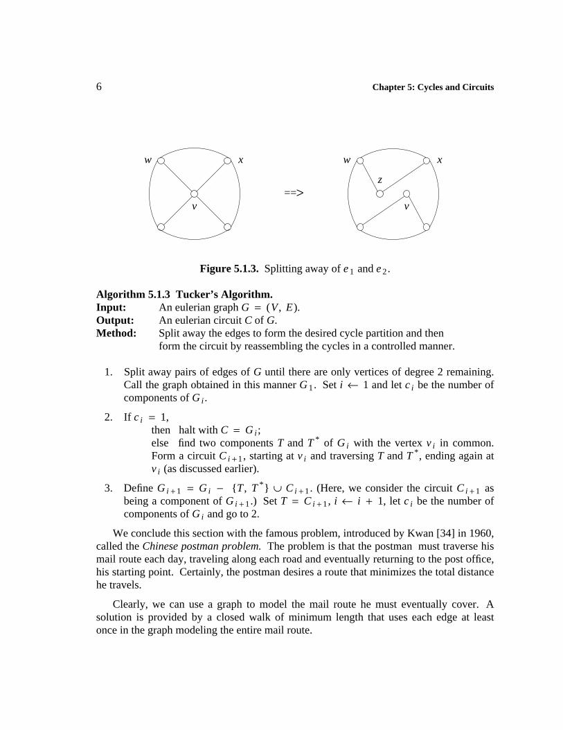
To verify this claim, suppose that a 1 and a 2 are two consecutive vertices of A on C.Since X ⊆ A, we may assume that a 1 and a 2 belong to some segment of C of the form[x i , x j ] (where 0 < i < j ≤ t) or [x t , x 1 ]. Let v ∈ N(x j ) and (letting v + be thesuccessor of v on C) let v + ∈ N(x k ) (x k ∈ (x j , x i )) where v and v + are in the segmentof vertices [a 1 , a 2 ]. Then, we see that x j is not x 0 or a longer cycle would exist. Infact, if x 0 v ∈ E(G), then v + x k ∈/ E(G) for any k, or a cycle longer than C would exist(see Figure 5.2.3 ). Furthermore, the vertices w i , w j , and w k cannot occur in that order


x 0

vv +

w kx k

Figure 5.2.3. Extending the cycle through x 0.

along C (according to its ordering), because again a cycle longer than C would exist (seeFigure 5.2.4). For example

x 0 , . . . , w k , . . . , x j , v , . . . , x k , v + , . . . , w j , x 0

is such an extension. Therefore,

N(x i ) , N(x i − 1 ) , N(x i − 2 ) , . . . , N(x 1 ) , N(x t ) , . . . , N(x i + 1 ) , N(x 0 )

form consecutive segments of vertices in the segment [ a 1 , a 2 ] (which is possiblyempty). Further, these segments have at most their end vertices in common. There aret + 1 segments; hence, there are at most t elements of D between a 1 and a 2. Thus, ourclaim is verified.

x 0

> a 1

v

v +

a 2

w jw k

x k

w i

x i

x j

Figure 5.2.4. The ordering of w i , w j , w k .


To complete the proof of the result, let x j , 0 ≤ j ≤ t be chosen with the maximumnumber s of neighbors in B. Then s ≥ ⎪B⎪/( t + 1 ). Also, the number of vertices of B inV(G) − V(C) equals n − m − ⎪A R⎪ (since two vertices of X have no commonneighbors in V(G) − V(C)). From our claim, the number of vertices of B on C is atleast m − ( t + 1 ) ⎪ A C ⎪. Thus,

⎪B⎪ = ⎪B ∩ C⎪ + ⎪B − C⎪

≥ n − m − ⎪A R⎪ + m − ( t + 1 ) ⎪A C⎪

= n − ⎪A R⎪ − ( t + 1 ) ⎪A C⎪

and

s ≥t + 1

⎪B⎪_ _____ ≥t + 1

n_ _____ −t + 1

⎪A R⎪_ _____ − ⎪A C⎪.

Since X − { x j } is a set of t mutually nonadjacent vertices and since ⎪A R⎪ ≥ 1,

⎪N(X − x j )⎪ = n − ⎪A⎪ − s = n − ⎪A R⎪ − ⎪A C⎪ − s

≤t + 1

t(n − ⎪A R⎪)_ ___________ ≤t + 1

t(n − 1 )_ ________ .

Hence, a contradiction is reached and the result is proved.

Example 5.2.2. The best known examples to show the sharpness of the bound in theprevious result are obtained by considering t + 1 copies of the complete graph K r whichare identified on a set of t vertices. The Petersen graph (see Figure 6.3.2) is anotherexample. However, these examples all leave some doubt as to the best possible lowerbound.

The graph tK r + K t satisfies the hypothesis of Fraisse’s Theorem, but its n-closureis itself. Thus, Theorem 5.2.6 is independent of the closure (Theorem 5.2.2).

It is interesting to note that the type of vertex set used can play a role here. In the lasttheorem independent sets of vertices were considered. However, something a bitdifferent happens if we consider arbitrary sets of vertices.

Theorem 5.2.7 [17] If G is a 2-connected graph of sufficiently large order n and if foreach pair of arbitrary vertices S = {a , b} we have that


⎪N(S)⎪ ≥2n_ _ ,


It is known that n > 10 suffices in Theorem 5.2.7. The Petersen graph is a smallorder (10) counterexample.

It is natural now to ask what happens if the set of vertices induces a clique? Whatproperties in general are important to the selection of the set? Some of these questionshave been considered, but the last and most important of them remains open. Theinterested reader should see [28] and [35] for more information.

Section 5.3 Related Hamiltonian-like Properties

In this section we wish to investigate several properties closely related to that ofbeing hamiltonian. Some of these are stronger properties, in the sense that the graphshaving these properties are also hamiltonian, while others are weaker. It is not surprisingthat truly applicable characterizations of these properties are not known. In some cases,very little is actually known at all about the classes of graphs we will describe.

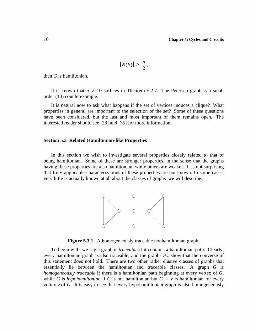
Figure 5.3.1. A homogeneously traceable nonhamiltonian graph.

To begin with, we say a graph is traceable if it contains a hamiltonian path. Clearly,every hamiltonian graph is also traceable, and the graphs P n show that the converse ofthis statement does not hold. There are two other rather elusive classes of graphs thatessentially lie between the hamiltonian and traceable classes. A graph G ishomogeneously traceable if there is a hamiltonian path beginning at every vertex of G,while G is hypohamiltonian if G is not hamiltonian but G − v is hamiltonian for everyvertex v of G. It is easy to see that every hypohamiltonian graph is also homogeneously


traceable. The graph of Figure 5.3.1 is homogeneously traceable, but nothypohamiltonian.

Skupien introduced homogeneously traceable graphs in [44], and the existence ofhomogeneously traceable nonhamiltonian graphs for all orders p ≥ 9 was shown in [6].In [32], Herz, Gaudin and Rossi showed that hypohamiltonian graphs exist, while in [31],Herz, Duby and Vigue ́ showed that there is no hypohamiltonian graph of order 11 or 12.Lindgren [37] and Sousselier (see [31]) independently showed that infinitely manyhypohamiltonian graphs exist. Both of these classes have remained elusive in the sensethat very few results are known about them, especially in view of the vast number ofresults known about hamiltonian graphs. Some simple facts will be explored in theexercises.

More success has been had with properties stronger than that of being hamiltonian.We say a graph G is hamiltonian connected if every two vertices of G are joined by ahamiltonian path. Clearly, every hamiltonian connected graph of order at least 3 ishamiltonian; the graphs C n (n ≥ 4 ) show that the converse is not true. We can use ageneralization of the idea of the closure to obtain a sufficient condition for a graph to behamiltonian connected. For a (p , q) graph G, let the (p + 1 )-closure denotedCL p + 1 (G), be that graph obtained from G by recursively joining pairs of nonadjacentvertices whose degree sum is at least p + 1. We obtain the following analog of Theorem5.2.4, also from Bondy and Chva ́ tal [4].

Theorem 5.3.1 Let G be a graph of order p. If CL p + 1 (G) is complete, then G ishamiltonian connected.

Proof. If p = 1, the result is clear. Thus, assume that p ≥ 2 and that G is a graph oforder p such that CL p + 1 (G) = K p . Let x and y be two vertices of G. We show that xand y are joined by a hamiltonian path in G, and since they are an arbitrary pair ofvertices, the result will follow.

Let H be the graph obtained from G by inserting a new vertex w and the edges wx andwy. Then H has order p * = p + 1.

Since deg H u + deg H v ≥ p * for all nonadjacent vertices u and v in G, it followsthat < V(G) > in CL(H) must be isomorphic to K p . Thus, if u ∈ V(G) anduw ∈/ E(H), then deg CL(H) u + deg CL(H) w ≥ p * , and, hence, CL(H) is isomorphic toK p * . Then by Ore’s theorem, H is hamiltonian. But any hamiltonian cycle in H mustcontain the edges wx and wy, and, thus, x and y are end vertices of a hamiltonian path inG.


The next two corollaries are analogs of the theorems of Ore and Dirac and areimmediate from our previous result, although they can also be proved directly.

Corollary 5.3.1 If G is a graph of order p such that for every pair of distinctnonadjacent vertices x and y in G, deg x + deg y ≥ p + 1, then G is hamiltonianconnected.

Corollary 5.3.2 If G is a graph of order p such that deg x ≥2

p + 1_ _____ for every vertex

x, then G is hamiltonian connected.

Yet another hamiltonian-like property is the following: A connected graphG = (V , E) is said to be panconnected if for each pair of distinct vertices x and y, thereexists an x − y path of length l , for each l satisfying d(x , y) ≤ l ≤ ⎪V⎪ − 1. If a graphG is panconnected, it is clearly hamiltonian connected and, thus, hamiltonian. It is alsoeasy to see that there are hamiltonian graphs that are not panconnected (for example,cycles). Can you find a graph that is hamiltonian connected but not panconnected? In aresult similar to Dirac’s theorem, Williamson [47] provided a sufficient condition for agraph to be panconnected in terms of minimum degree.

Theorem 5.3.2 If G is a graph of order p ≥ 4 such that for every vertex x ∈ V(G),

deg x ≥2

p + 2_ _____, then G is panconnected.

Our final properties are somewhat related. We say a graph G of order p is pancyclicif it contains a cycle of every length l, ( 3 ≤ l ≤ p). We say G is vertex pancyclic if eachvertex of G lies on a cycle of each length l, ( 3 ≤ l ≤ p). Clearly, every pancyclic andevery vertex pancyclic graph is hamiltonian. It is also clear that every vertex pancyclicgraph is pancyclic. Can you find a graph that is pancyclic, but not vertex pancyclic? Asufficient condition for a graph to be pancyclic was provided by Bondy [3].

Theorem 5.3.3 If G is a hamiltonian (p , q) graph with q ≥4

p 2_ __, then either G is

pancyclic or p is even and G is isomorphic to K p /2 , p /2.

Many hamiltonian results, similar to those we have studied, exist for digraphs. Weexplore some of these in the exercises.


Section 5.4 Forbidden Subgraphs

In this section we consider another approach that has seen considerable study.Goodman and Hedetniemi [27] noticed that forbidding particular induced subgraphsoffered a new type of hamiltonian result. If F = {H 1 , . . . , H k } is a family of graphs,we say that G is F-free if G does not contain any of the graphs in the set F as an inducedsubgraph. If F is a single graph H we simply say that G is H-free. We defineZ 1 = K 1 , 3 + e.

Theorem 5.4.1 ([27]) If G is a 2-connected { K 1 , 3 , Z 1}-free graph, then G ishamiltonian.

Proof. Suppose G is not hamiltonian. Since G is 2-connected, it contains cycles. LetC : x 1 , x 2 , . . . , x n , x 1 be a cycle in G of maximum length. Then, there must exist avertex x not on C that is adjacent to a vertex, say x i , of C. Then, < x , x i , x i − 1 , x i + 1 >induces either a K 1 , 3 or a Z 1, unless at least two of the edges xx i − 1, xx i + 1, or x i − 1 x i + 1are present in G. But then no matter how these edges are selected, one of xx i − 1 or xx i + 1must be present, and a cycle longer than C is produced, a contradiction to our choice ofC. Thus, G is hamiltonian.

Theorem 5.4.1 inspired several others. One of the earliest and strongest of these isnow stated. The graph N (known as the net) is seen in Figure 5.4.1.

Figure 5.4.1. The graph N.

Theorem 5.4.2 ([12]) If G is

1. connected and {K 1 , 3 , N}-free, then G is traceable.

2. 2-connected and {K 1 , 3 , N}-free, then G is hamiltonian.


Note that if H is an induced subgraph of some graph S and G is H-free, then G is alsoS-free, for if G contained an induced S, it clearly would contain an induced H as well.Thus, we get the following corollary to Theorem 5.4.2. The graph B is shown in Figure5.4.2.

Corollary 5.4.1 If G is a 2-connected graph that is {R , S}-free where R = K 1 , 3 and Sis any one of N, C 3, Z 1, B, P 4, P 3, K 2 or K 1, then G is hamiltonian.

In the list of graphs given in Corollary 5.4.1, we note that if P 3 is forbidden, thegraph must clearly be complete, thus it has any hamiltonian property you wish. Further,if the induced subgraphs of P 3 are forbidden, namely K 2 or K 1, we either have that Gmust be K 1 or G is empty. In either case we arrive at trivial cases that satisfy allhamiltonian properties. For this reason in what remains we will ignore P 3 and itsinduced subgraphs as simply being trivial and therefore "uninteresting".

Z 3

W B

Figure 5.4.2. Common forbidden subgraphs.

After Theorem 5.4.2 was announced, the search for other familes of forbiddensubgraphs began in earnest. Over the course of the next decade a variety of such resultswere discovered. We summarize the most important of these for our purposes in the nextresult. See Figure 5.4.2 for the graphs W and Z 3, where by Z i we mean a triangle with apath containing exactly i edges from one of its vertices.

Theorem 5.4.3 If G is a 2-connected graph and G is

i. ([5]) {K 1 , 3 , P 6}-free, or


ii. ([2]) {K 1 , 3 , W}-free, or

iii. ([20]) {K 1 , 3 , Z 3}-free and of order p ≥ 10,then G is hamiltonian.

Recently, a characterization of all pairs of graphs that, when forbidden, imply a 2-connected graph is hamiltonian was given in [16].

...

G 1

.

..

G 0

K m

K m

K m

G 2

K m

G 3

K m

e 1 e 2 e 3

G 4

K m

G 6G 5

Figure 5.4.3. 2-Connected, nonhamiltonian graphs.


Theorem 5.4.4 Let R and S be connected graphs (R , S ≠ P 3 ) and G a 2-connectedgraph of order n ≥ 10. Then G is (R , S)-free implies G is hamiltonian if, and only if,R = K 1 , 3 and S is one of the graphs C 3, P 4, P 5, P 6, Z 1, Z 2, Z 3, B, N or W.

Proof: That each of the pairs implies G is hamiltonian follows from Theorems 5.4.2 and5.4.3 and our earlier remarks about induced subgraphs of forbidden graphs.

Now consider the graphs G 0 , . . . , G 6 of Figure 5.4.3. Each is 2-connected andnonhamiltonian (and really represents an infinite family of such graphs). Without loss ofgenerality assume that R is a subgraph of G 1.

Case 1: Suppose that R contains an induced P 4.

Since G 4, G 5, and G 6 are all P 4-free, then S must be an induced subgraph of each ofthem. But if S is an induced subgraph of G 4, then either S is a star or S contains aninduced C 4. However, G 5 is C 4-free, hence S must be a star. Since the only inducedstar in G 6 is K 1 , 3 , we have that S = K 1 , 3 .

Case 2: Suppose that R does not contain an induced P 4.

Then, using G 0 we see immediately that R must be a tree containing at most onevertex of degree 3 and since R contains no induced P 4, we see that R = K 1 , 3 . Thus, forthe remainder of the proof we assume without loss of generality that R = K 1 , 3 .

Now, S must be an induced subgraph of G 1, G 2, and G 3 (each of which is claw-free).The fact that S is an induced subgraph of G 1 implies that S is a path or S is K 3, possiblywith a path off each of its vertices. Suppose that S is a path. Since S is an inducedsubgraph of G 3 which is P 7-free, we see that if S is a path, it is one of P 4, P 5 or P 6.

We now assume that S contains a K 3, possibly with a path off each of its vertices.Note that G 3 is Z 4-free. Further, any triangle in G 2 with a 3-path off one of its verticescan have no paths off its other vertices (leaving Z 3, Z 2, Z 1, and K 3). Again examiningG 2 we see it contains no triangle with a path of length 2 from one of its vertices and apath of length 1 from the other two vertices. Next, the graph G * 3 obtained by deletingthe three edges e 1, e 2 and e 3 from G 3 is still claw-free and contains no induced K 3 witha 2-path from two vertices. (leaving B or W). The only remaining possibility is a path oflength 1 off each of the vertices of K 3, that is, the graph N.

Note that similar results are known for traceable graphs as well as for several otherhamiltonian type properties. These will be explored in more detail in the exercises.


Section 5.5 Other Types of Hamiltonian Results

In this section we wish to consider several other types of results concerninghamiltonian and hamiltonian-like graphs. These use conditions that are often verydifferent from those we have seen thus far. We begin with an investigation of the powersof a graph.

The nth power G n of a connected graph G is that graph with V(G n ) = V(G) and inwhich uv is an edge of G n if, and only if, 1 ≤ d G (u , v) ≤ n. The graphs G 2 and G 3 arecalled the square and cube of G , respectively. Figure 5.5.1 shows the subdivision graphof the graph K 1 , 3 , that is, the graph S(K 1 , 3 ) obtained by subdividing each edge ofK 1 , 3 . The graph S(K 1 , 3 ) is formed from K 1 , 3 when each edge e = xy is removed anda new vertex w is inserted along with the edges wx and wy. Figure 5.5.1 also shows thesquare of S(K 1 , 3 ).

Since higher powers of a graph G tend to contain more edges than G itself, it isreasonable to ask if these powers will eventually become hamiltonian, even if G is not.Nash-Williams and Plummer conjectured that this was indeed the case for the squares of2-connected graphs. In the now classic paper [21], Fleischner verified that this wasindeed the case.

G = S( K 1 , 3 ) G 2

Figure 5.5.1. The graph S(K 1 , 3 ) and its square.

Theorem 5.5.1 Let G be a 2-connected graph. Then G 2 is hamiltonian.

The proof of Fleischner’s theorem is beyond the scope of most texts and, hence, willnot be presented. However, this work opened the door for others to investigate properties


in powers of graphs. In [7], Fleischner’s result was strengthened to show that the squareof every 2-connected graph is actually hamiltonian connected (see the exercises).

Let us switch attention now to hamiltonian properties of line graphs. In [30], Hararyand Nash-Williams characterized when the line graph L(G) of a graph G is hamiltonian.In order to do this, we define a dominating circuit C of a graph G to be a circuit with theproperty that every edge of G is incident to a vertex of C.

Theorem 5.5.2 Let G be a graph without isolated vertices. Then L(G) is hamiltonianif, and only if, G is isomorphic to K 1 , n (n ≥ 3) or G contains a dominating circuit.

The major impact of Theorem 5.5.2 has been its use in proving other results.

In [29], the idea of dominating circuits is used to help establish a result that combinesideas from throughout this section. Suppose that H is a connected graph and that L(H) isnot hamiltonian. Therefore, H must not contain a dominating circuit. Among all circuitsof H, let C be one with the maximum number of vertices. Let V = V(C) and letU = V(H) − V. Since C is not a dominating circuit, < U > is not an empty graph.Thus, since H is connected, there exists at least one edge from U to V in H. With this inmind, we present the following lemma [29].

Lemma 5.5.1 No U − V edge of H lies on a triangle T of H.

Proof. Suppose that the result failed to hold; then one of the following cases would haveto occur.

Case 1: Exactly one vertex of the triangle T lies on C and, thus, a circuit longer thanC would exist, a contradiction.

Case 2: Exactly two vertices of the triangle T lie on C and they are consecutive on C(say they are joined by e). Then deleting e and inserting the other two edges of T createsa circuit longer than C, again a contradiction.

Case 3: Exactly two vertices of T lie on C, but these two vertices are not consecutive.Then a longer circuit can be found using all of C and all of T, once again producing acontradiction.

This completes the cases, and, thus, the lemma follows.

Using this lemma, we can obtain a result concerning hamiltonian properties in thesecond iterated line graph of a graph [29].


Theorem 5.5.3 Let G be a connected graph of order p ≥ 3 which does not contain avertex cutset consisting only of vertices of degree 2. Then L 2 (G) (that is, L(L(G) )) ishamiltonian.

Proof. Let H = L(G) and suppose that L(H) = L 2 (G) is not hamiltonian. Then, asabove, there exists a partition of V(H) as V ∪ U such that (by the lemma) no U − Vedge in H lies on a triangle. Let e 1 f 1 , . . . , e r f r (r ≥ 1 ) be the U − V edges in H andlet v i be the common end vertex of e i and f i in G ( 1 ≤ i ≤ r). Since e i f i does not lie ina triangle of H, deg G v i = 2, ( 1 ≤ i ≤ r). Further, since the graph

H − { e i f i ⎪ 1 ≤ i ≤ r }

is disconnected, then G − { v i ⎪ 1 ≤ i ≤ r } is also disconnected. Therefore, we reacha contradiction since { v i ⎪ 1 ≤ i ≤ r } is a cut set of G consisting entirely of vertices ofdegree 2. Thus, the result follows.

With the aid of Theorem 5.5.3, the following corollary, originally from Chartrand andWall [8], is immediate.

Corollary 5.5.1 If G is a connected graph such that δ(G) ≥ 3, then L 2 (G) ishamiltonian.

Section 5.6 The Traveling Salesman Problem

Consider the dilemma of a traveling salesman. He must visit each city in his regionand return to his home office on a regular basis. He seeks the route that allows him tovisit each city at least once (exactly once would be even better) and return home, with theadded property that this route also covers the least distance. Clearly, a weighted graphcan be used to model the possible routes. Because we can insert edges with infinitedistances, we can also restrict our attention to complete graphs.

Unfortunately for the traveling salesman, this problem is NP-complete (see, forexample, [24]). Thus, efforts have concentrated on approximation algorithms and the useof heuristics to try to make some gains. The heuristic one usually thinks of first, thenearest neighbor approach, begins with a single vertex, adds the edge of minimumdistance, and continues by trying to build from either end of this path by repeatedlytaking the nearest neighbor. Unfortunately, to close the path into a cycle is often veryexpensive, and we can also ignore many short edges this way. Thus, this approach isvery unreliable.


To try to overcome this difficulty, you might try beginning with some short cycle andexpand this cycle by inserting the vertex that causes the cycle length to increase the least.This technique is called the shortest insertion heuristic. Once again, difficulties can arise.Part of the problem stems from the fact that an arbitrarily weighted graph need not satisfythe "reasonable rules" of distance. That is, the triangle inequality need not hold.However, if the triangle inequality does hold, some progress can be made. In thealgorithm that follows, we assume both a single vertex and a K 2 are (degenerate) cycles.

Algorithm 5.6.1 The Shortest Insertion AlgorithmInput: A weighted graph G = (V , E) satisfying the triangle

inequality.Output: A hamiltonian cycle C that approximates the salesman cycle.

1. Select any vertex and consider it a 1-cycle C 1 of G. Set i ← 1.

2. If i = p, then halt since C = C p is the desired cycle;else if C i has been selected ( 1 ≤ i ≤ p), then find a vertex v i not on C i that isclosest to a consecutive pair of vertices w i and w i + 1 of C i .

3. Let C i + 1 be formed by inserting v i between w i and w i + 1 on C i and go to step 2.

The type of heuristics we have just considered constructs a tour whose value is hopedto be close to optimal. These are known as tour construction heuristics. Other heuristicstake a tour and try to improve it (known as tour improvement heuristics). One of themost commonly used improvement procedures is that of edge exchanges.

In general, r edges in a tour are exchanged for r edges not in the tour, as long as theresult remains a tour and the length of the new tour is less than the length of the old tour.Exchange procedures have come to be called r-opt procedures, where r is the number ofedges exchanged at each iteration. Figure 5.6.1 illustrates the exchange for 2-opt and 3-opt.

In an r-opt algorithm, all feasible exchanges of r edges are tested until there is noexchange that improves the current situation. The solution is than said to be r-optimal(see [36]). In general, the larger the value of r, the more likely it is that the final tour isoptimal. However, the number of operations necessary to test all possible r exchangesincreases dramatically as the number of cities increase. For this reason, r = 2 and r = 3are the most commonly used values.


Figure 5.6.1. The 2-opt and 3-opt exchanges

Section 5.7 Short Cycles and Girth

In this section we explore a few results about nonhamiltonian cycles in graphs. Manyof the same techniques that aided us in finding spanning cycles can be of use here. Webegin with a result from [4].

Theorem 5.7.1 If G is a graph of order p ≥ 3 and 5 ≤ t ≤ p, then the graph Gcontains a C t if, and only if, for every pair of nonadjacent vertices u and v such thatdeg u + deg v ≥ 2p − t, G + uv contains a C t .

Proof. If G contains C t , then clearly so does G + uv.

To prove the converse, suppose that G + uv contains a C t , but G does not. Thenthere exists a path P of length t − 1 in G joining u and v. Let U = V(G) − V(P).Then it is clear that ⎪U⎪ = p − t. If u and v are each adjacent to all of U, then that stillaccounts for only 2 (p − t) adjacencies. Thus, they must have at least t adjacencies on P.But now, we simply apply the technique used in the proof of Ore’s theorem to produce aC t using the vertices of P.

We may also use neighborhoods to obtain results about nonspanning cycles.

Theorem 5.7.2 ([19]) If G is 2-connected of order p satisfying the property that forevery pair of nonadjacent vertices u and v

⎪N(u) ∪ N(v)⎪ ≥ s,then G contains a cycle of length at least s + 2 or (if p < s + 2) G is complete.

Proof If p < s + 2, then the neighborhood condition implies that G must be complete.


Now, assume that p ≥ s + 2. Let G be a 2-connected graph of order p satisfying theneighborhood condition. Let x 1 , x 2 , . . . , x t be the vertices in order along a path P ofmaximum length in G. Let x i and x j (possibly i = j) be vertices on P that are adjacentto x 1, and suppose that, among all possible longest paths P and vertices x i , we havechosen ones that maximize i. Then x 1 and x j − 1 are adjacent only to vertices in

W = { x 1 , . . . , x i }(since clearly x j − 1 is an end vertex of a path having the same length as P). Supposei ≤ s + 1. Then by the neighborhood condition, we see that x 1 and x j − 1 must beadjacent. Taking j to be i , i − 1 , . . . in turn, we see that x 1 is adjacent to each ofx 2 , . . . , x i . All vertices x 1 , . . . , x i − 1 are, thus, end vertices of paths of the samelength as P, and so they are adjacent only to vertices of W, which contradicts the 2-connectedness of G. Thus, i ≥ s + 2, and G contains a cycle of length s + 2 or more.

We now turn our attention specifically to the shortest cycle in a graph. The girth of agraph G, denoted g(G), is the length of a shortest cycle in G. We can bound the order ofG from below using the girth and the minimum degree of G. Let f (g , δ) be theminimum order of a graph G with g(G) ≥ g and δ(G) ≥ δ. It is not immediatelyobvious that there exist graphs satisfying these restrictions. We shall provide an upperbound on f (g , δ) (and, hence, prove the existence of such graphs) in Chapter 9 usingprobabilistic techniques. For now, we shall accept their existence and try to learn moreabout them. One can obtain an easy lower bound on f (g , δ).

Theorem 5.7.3 For δ , g ≥ 3,

f (g , δ) ≥

⎧⎪⎪⎨⎪⎪⎩

δ − 2( δ − 1 ) d − 1_ _____________ if g = 2d.

δ − 2δ( δ − 1 ) d − 2_ _______________ if g = 2d + 1 ,

(5.7.1)

Proof. If g is odd, say g = 2d + 1, note that the subgraph induced by those verticeswithin a distance d of a vertex x must be a tree, since any cycle within this graph wouldhave length less than g. Since there are at least δ(δ − 1 ) j vertices at distance j + 1from x, we see that


f (g , δ) ≥ 1 + δj = 0Σd

(δ − 1 ) j .

Since this is a geometric series, the desired result follows.

Now, suppose that g is even, say g = 2d. Then consider the vertices within adistance d of the edge xy and proceed in a manner similar to the odd case to obtain thebound.

In certain cases we can find the exact value of f (g , δ), especially when the graph isδ-regular. For example, the 2-regular graphs of girth g and minimum order p are simplythe cycles C p . It is also easy to see that the r-regular graphs of girth g = 3 andminimum order are simply the complete graphs K r + 1. When g = 4 and the graph is r-regular, then the complete bipartite graphs K δ, δ have minimum order and theseconditions. It has become common to call r-regular graphs of girth g and minimum orderthe (g , r)-cages. It turns out that (g , r)-cages are difficult to find. The first reallyinteresting case is the ( 5 , 3 )-cage; that is, we want a 3-regular graph of girth 5 andminimum possible order. Using our tree structure (from the proof of Theorem 5.7.3), wesee that such a graph has at least 10 vertices. The graph of Figure 5.7.1 has exactly 10vertices and satisfies the other conditions as well (a fact you must convince yourself of).The interesting point here is that this graph is isomorphic to the Petersen graph and is theunique ( 5 , 3 )-cage (see the exercises).

Figure 5.7.1. The ( 5 , 3 )-cage.

We next state a result summarizing some of the best known work on boundingf (g , δ).

Theorem 5.7.4

1. For δ ≥ 2, f ( 4 , δ) = 2δ.


2. For δ ≥ 2, f (g , δ) ≥ δ2 + 1. Furthermore, for δ ≠ 57, equality holds if, andonly if, δ = 2 , 3 or 7.

3. When δ = p m + 1, for some prime p and positive integer m, then

f ( 6 , δ) =δ − 2

2 (δ − 1 )3 − 2_ _____________ .

We conclude with a table of orders for the known cages (Table 5.7.1).

_ ________________________________________r/g 5 6 7 8 9 12_ ________________________________________3 10 14 24 30 126_ ________________________________________4 19 26_ ________________________________________5 30 40 50_ ________________________________________ ⎜⎜

⎜⎜⎜⎜

⎜⎜⎜⎜⎜⎜

⎜⎜⎜⎜⎜⎜

⎜⎜⎜⎜⎜⎜

⎜⎜⎜⎜⎜⎜

⎜⎜⎜⎜⎜⎜

⎜⎜⎜⎜⎜⎜

⎜⎜⎜⎜⎜⎜

Table 5.7.1 Known orders for cages.

Section 5.8 Disjoint Cycles

In this section we wish to explore the situation of when several cycles may be foundin a graph. At this point in time we only care that these cycles are disjoint (both verticesand edges). We begin with a result due to Po ´sa [43]. Our concern is in finding a pair ofvertex disjoint cycles of unspecified order. We define s(n) to be the minimum number ofedges so that every graph on n vertices contains two vertex disjoint cycles.

Theorem 5.8.1 For n ≥ 6 , s(n) = 3n − 5.

Proof. We first note that 3n − 6 edges is not enough to guarantee the existence of twovertex disjoint cycles. To see this, we need only consider K 1 , 1 , 1 , n − 3 and note that anycycle in this graph must use at least two of the vertices in the partite sets of cardinality 1.Hence, two disjoint cycles cannot exist.

To establish that every (n , 3n − 5 ) graph must contain two disjoint cycles, weproceed inductively on n. For n = 6, we note that 3n − 5 = 13. This means that thegraph in question is K 6 minus two edges. It is easy to check that no matter how thesetwo edges are deleted, two vertex disjoint triangles remain.


Now, assume the result is true for all such graphs of order less than n and consider an(n , 3n − 5 ) graph G. Since Σ deg v i = 6n − 10 , we see that G must have a vertexof degree at most 5. Call such a vertex x. We now consider cases for the possible valuesof deg x.

Suppose that deg x = 5 and let N(x) = { v 1 , v 2 , . . . , v 5 } . If⎪ E( <N[x] >) ⎪ ≥ 13, then as in the anchor step, G contains two disjoint triangles.Otherwise, some v i , say v 1, has two nonadjacencies in N(x). Without loss of generality,say v 1 is not adjacent to v 2 and v 3.

Now, consider the graph H = G − x + { v 1 v 2 , v 1 v 3 }. Note that H is an(n − 1 , 3n − 8 ) graph and so by the induction hypothesis, H must contain two disjointcycles, say C 1 and C 2 . If C 1 and C 2 do not use the edges we inserted to form H, thenthey must also exist in our original graph G. Thus, since at most one of these cycles canuse the edges we inserted, we must have one cycle intact inside G. We now wish to showthat the other cycle from H can be modified to form a second cycle in G.

If this cycle uses v 1 v 2 (or v 1 v 3) only, then replacing this edge with the vertex x andedges v 1 x, xv 2 produces the desired cycle in G. If both v 1 v 2 and v 1 v 3 are used, replacethem with x and xv 2, xv 3 to form the desired cycle. In any case, two disjoint cycles in Gare found.

If deg x = 4, a similar argument applies. If deg x ≤ 3, then when x is removed fromG, no other edges need be added to be able to apply the inductive hypothesis, and twodisjoint cycles are found in G − x immediately. Thus, in all cases, the result holds.

This result is sharp since the graph K 3 + nK 1 has p = n + 3 vertices, 3p − 6edges and does not contain 2 disjoint cycles.

For K 1 , 3-free graphs, Matthews [38] proved that if q ≥ p + 6, then the graphcontains 2 disjoint cycles. We will prove a weaker (and much shorter) result.

Theorem 5.8.2 If G is a (p , q) K 1 , 3-free graph with q ≥ p + 6, then G contains 2disjoint cycles or Δ(G) < 6.

Proof: Suppose that Δ(G) ≥ 6 and also that the result fails, hence any two cycles in Gintersect. Since deg u ≥ 6 for some vertex u, then by Theorem 1.6.2 and the fact that Gis K 1 , 3-free, we see that N(u) must contain a triangle, say T. But u and any three of theremaining vertices in N(u) − V(T) cannot induce a K 1 , 3 , thus a triangle disjoint from Texists.


This result is also sharp since the graph K 5 with a path of length n attached to anyone of its vertices has p + 5 edges, is K 1 , 3-free and does not contain 2 disjoint cycles.

For the case of finding k disjoint cycles, it was shown in [14] that for k ≥ 1 andp ≥ 24k, then every graph with q ≥ ( 2k − 1 ) p − 2k 2 + k contains either k disjointcycles or G = K 2k − 1 + (p − 2k + 1 ) K 1. This result was improved for K 1 , 3-freegraphs by Chen, Markus and Schelp [9].

Theorem 5.8.3 Let G be a K 1 , 3-free graph and let k ≥ 1. If

q ≥ p + ( 3k − 1 ) ( 3k − 4 )/2 + 1

then G contains k disjoint cycles.

Finally, Corra ́ di and Hajnal [10] showed the following.

Theorem 5.8.4 If G is an (n ,q) graph with n ≥ 3k and δ(G) ≥ 2k, then G contains kdisjoint cycles.

Exercises

1. Prove Corollary 5.1.2.

2. Prove Theorem 5.1.2.

3. Determine the complexity of Algorithm 5.1.1.

4. Use each of Algorithms 5.1.1, 5.1.2 and 5.1.3 to find an eulerian cycle in the graphbelow.

5. Determine an algorithm to accomplish the splitting away of two edges.

6. If H is the graph obtained from G by splitting away e 1 = vw and e 2 = vx, provethat H is connected if, and only if, G is connected and { e 1 , e 2 } does not form acut set.


7. Prove that a nontrivial connected graph G is eulerian if, and only if, every edge ofG lies on an odd number of cycles.

8. Prove that a nontrivial connected digraph D is eulerian if and only if E can bepartitioned into subsets E 1 , E 2 , . . . , E k such that the graph induced by E i is acycle for each i, ( 1 ≤ i ≤ k).

9. Prove Observations 1 and 2.

10. Show that if G = (V , E) is hamiltonian, then for every proper subset S of V, thenumber of components in G − S is at most ⎪S⎪.

11. Show that if G is not 2-connected, then G is not hamiltonian.

12. Characterize when the graph K p 1 ,p 2 , . . . , p nis hamiltonian.

13. Prove or disprove: If G and H are hamiltonian, then G × H is hamiltonian.

14. Prove or disprove: If G and H are hamiltonian, then G[H] is hamiltonian.

15. Let the n-cube be the graph Q n = K 2 × Q n − 1 (where Q 1 = K 2). Prove that ifn ≥ 2, Q n is hamiltonian.

16. Let G be a graph with δ(G) ≥ 2. Show that G contains a cycle of length at leastδ(G) + 1.

17. Suppose that G is a (p , q) graph with p ≥ 3. Show that if q ≥2

p 2 − 3p + 6_ ____________,


18. Show that if G is a (p , q) graph with q ≥ ( 2

p − 1 ) + 3, then G is hamiltonian

connected.

19. Show that if G is hamiltonian connected, then G is 3-connected.

20. Show that if a (p , q) graph G is hamiltonian connected and if p ≥ 4, then

q ≥⎪⎪⎣ 2

3p + 1_ ______⎪⎪⎦.

21. Give an example of a graph that is pancyclic but not panconnected.

22. Find an example of a graph that is hamiltonian connected but not panconnected.

23. Find an example of a graph that is pancyclic but not vertex pancyclic.


24. Can we remove the restriction that D be strongly connected from Meyniel’stheorem?

25. Show that every complete graph with directed edges is traceable.

26. Show that K n with strong directed edges is vertex pancyclic.

27. Give an example of a hamiltonian connected digraph that satisfies the conditions of

Theorem 5.4.2 but does not have od v ≥2

p + 1_ ____ and id v ≥2

p + 1_ ____ for every vertex

v.

28. Show that the Petersen graph is homogeneously traceable nonhamiltonian and alsohypohamiltonian.

29. Show that homogeneously traceable nonhamiltonian graphs exist for all ordersp ≥ 9.

30. Show that if G = (V , E) is a homogeneously traceable nonhamiltonian graph andx ∈ V, then x is adjacent to at most one vertex of degree 2.

31. Show that if C p − 1 (G) = K p , then G is traceable.

32. Prove Corollary 5.4.2.

33. Prove that the graph G 2 of Figure 5.5.1 is not hamiltonian.

34. Show (without using Fleischner’s theorem) that if G is 2-connected, then G 3 ishamiltonian. (Hint: Consider spanning trees).

35. Use Fleischner’s theorem to show that if G is 2-connected, then G 2 is hamiltonianconnected. (Hint: Consider five copies of G along with two additional vertices xand y joined to an arbitrary pair of vertices u and v in each copy of G).

36. Prove Theorem 5.5.2.

37. Prove that if G is a graph of order p ≥ 3 such that the vertices of G can be labeledv 1 , v 2 , . . . , v p so that

deg v j ≤ j , deg v k ≤ k − 1j < k , j + k ≥ p , v j v k ∈/ E(G)

deg v j + deg v k ≥ p.


38. Let G be a graph of order p ≥ 3, the degrees d i of whose vertices satisfyd 1 ≤ d 2 ≤ , . . . , ≤ d p . If

d j ≤ j <2p_ _ d p − j ≥ p − j,



39. Prove that if G is a graph of order p ≥ 3 such that for every integer j with

1 ≤ j <2p_ _, the number of vertices of degree not exceeding j is less than j, then G

is hamiltonian.

40. Prove that if G has order p ≥ 3 and if k(G) ≥ β(G) = the maximum number ofmutually nonadjacent vertices, then G is hamiltonian.

41. (Ghouila-Houri [25]) Let D be a strongly connected digraph such that deg x ≥ pfor every vertex x of D. Prove D is hamiltonian.

42. (Woodall [48]) Let D be a digraph of order p ≥ 3 such that whenever x and y aredistinct vertices and x → y is not an arc of D, then od x + id y ≥ p. Prove D ishamiltonian.

43. (Meyniel [39]) Let D be a strongly connected digraph of order p ≥ 3 such thatfor every distinct pair of nonadjacent vertices x and y, deg x + deg y ≥ 2p − 1.Prove D is hamiltonian.

44. (Overbeck-Larisch [42]) Let D be a digraph of order p ≥ 2 such that for everypair of distinct vertices x and y such that x → y is not an arc of D,od x + id y ≥ p + 1. Prove D is hamiltonian connected.

45. Determine all pairs of graphs (R , S) that when forbidden, imply a 2-connectedgraph is pancyclic.

46. Determine all pairs of graphs (R , S) that when forbidden, imply a 2-connectedgraph is panconnected.

47. Determine all pairs of graphs (R , S) that when forbidden, imply a connected graphis traceable.

48. Show that the only single graph that when forbidden, implies a 2-connected graphis hamiltonian, is P 3.

49. Determine the minimum salesman’s walk in the following graph.


3

2

1

1

2

4 2

4

4

3 1

50. Show that the greedy approach to the traveling salesman problem can be arbitrarilybad.

51. Prove that the graph of Figure 5.7.1 is the unique ( 5 , 3 )-cage and is isomorphic tothe Petersen graph.

52. Find the ( 6 , 3 )-cage and show that it is unique.

53. Prove Theorem 5.7.4(1).

54. Prove that if G is a K 1 , 3-free graph that does not contain k disjoint cycles, thenΔ(G) ≤ 3k − 1.

55. Prove that if G is a K 1 , 3-free graph with Δ(G) ≤ 5 that G contains two disjointcycles.

56. Prove that if a (p , q)-graph G is K 1 , 3-free, k ≥ 1 andq ≥ p + ( 3k − 1 ) ( 3k − 4 )/2 + 1, then G contains k disjoint cycles.

References

1. Albertson, M. O., Finding Hamiltonian Cycles in Ore Graphs, preprint.

2. Bedrossian, P., Forbidden Subgraph and Minimum Degree Conditions forHamiltonicity, Ph.D. Thesis, Memphis State University, 1991.

3. Bondy, J. A., Pancyclic Graphs. J. Combin. Theory, 11B(1971), 80 − 84.

4. Bondy, J. A., and Chva ́ tal, V., A Method in Graph Theory. Discrete Math.15(1976), 111 − 136.

5. Broersma, H.J., Veldman, H.J., Restrictions on Induced Subraphs EnsuringHamiltonicity or Pancyclicity of K 1 , 3-free Graphs, Contemporary Methods inGraph Theory (R. Bodendiek), BI-Wiss.-Verl., Mannheim-Wien-Zurich, (1990)181 − 194.


6. Chartrand, G., Gould, R. J., and Kapoor, S. F., On Homogeneously TraceableNonhamiltonian Graphs. Annals of the N. Y. Acad. of Sci., Vol. 319(1979),130 − 135.

7. Chartrand, G., Hobbs, A., Jung, A., Kapoor, S.F., and Nash-Williams, C. St. J. A.,The Square of a Block is Hamiltonian Connected. J. Combin. Theory, 16B(1974),290 − 292.

8. Chartrand, G. and Wall, C. E., On the Hamiltonian Index of a Graph. Studia Sci.Math. Hungar., 8(1973), 43 − 48.

9. Chen, G., Markus, L.R., and Schelp, R. H., Vertex Disjoint Cycles for Star FreeGraphs. Australasian J. of Combinatorics, 11(1995) 157-169.

10. Corra ́ di, K. and Hajnal, A., On the Maximal Number of Independent Circuits in aGraph. Acta Math. Acad. Sci. Hungar., 14(1963), 423 − 439.

11. Dirac, G. A., Some Theorems on Abstract Graphs. Proc London Math. Soc.,2(1952), 69 − 81.

12. Duffus, D., Gould, R. J., and Jacobson, M. S., Forbidden Subgraphs and theHamiltonian Theme. The Theory and Applications of Graphs, Ed. by Chartrand etal., Wiley-Interscience, New York (1981), 297 − 316.

13. Edmonds, J., and Johnson, E. L., Matching, Euler Tours and the Chinese Postman.Math. Programming, 5(1973), 88 − 124.

14. Erdo. .s, P. and Po ´sa, L., On the Maximal Number of Disjoint Circuits of a Graph,

Math. Debrecen 9 (1962), 3 − 12.

15. Euler, L., Solutio Problematis ad Geometriam Situs Pertinentis. Comment.Acadamiae Sci. I. Petropolitanae, 8(1736), 128 − 140.

16. Faudree, R.J., Gould, R.J., Characterizing Forbidden Pairs for HamiltonianProperties, Discrete Math. (to appear).

17. Faudree, R.J., Gould, R.J., Jacobson, M.S. and L. Lesniak, Neighborhood Unionsand a Generalization of Dirac’s Theorem. Discrete Math. 105, (1992), 61 − 71.

18. Faudree, R. J., Gould, R. J., Jacobson, M. S., and Schelp, R. H., NeighborhoodUnions and Hamiltonian Properties of Graphs. J. Combin. Theory B (in press).

19. Faudree, R. J., Gould, R. J., Jacobson, M. S., and Schelp, R. H., Extremal ProblemsInvolving Neighborhood Unions. J. Graph Theory, 11 (1987), 555 − 564.


20. Faudree, R.J., Gould, R.J, Ryjacek, Z., Schiermeyer, I., Forbidden Subgraphs andPancyclicity (preprint).

21. Fleischner, H., The square of Every Two-Connected Graph is Hamiltonian. J.Combin. Theory, 16B(1974), 29 − 34.

22. Fleury [see Lucas, E., Recreations Mathematiques IV, Paris, 1921].

23. Fraisse, P., A New Sufficient Condition for Hamiltonian Graphs. J. GraphTheory, 10(1986), 405 − 409.

24. Garey, M. R., and Johnson, D. S., Computers and Intractability. W. H. Freemanand Co., San Francisco (1979).

25. Ghouila-Houri, A., Une Condition Suffisante d’existence d’un Circuit Hamiltonien.C. R. Acad. Sci. Paris, 156(1960), 495 − 497.

26. Goodman, S. E., and Hedetniemi, S. T., Eulerian Walks in Graphs. SIAM J.Comput., 2(1973), 16 − 27.

27. Goodman, S. E., and Hedetniemi, S. T., Sufficient Conditions for a Graph to beHamiltonian. J. Combin. Theory, B(1974), 175 − 180.

28. Gould, R. J., Updating the Hamiltonian Problem - A Survey, Journal of GraphTheory, Vol. 15, No. 2, (1991), 121-157.

29. Gould, R. J., and Hendry, G., personnel communication (1984).

30. Harary, F., and Nash-Williams, C. St. J. A., On Eulerian and Hamiltonian Graphsand Line Graphs. Canad. Math. Bull., 8(1965), 701 − 710.

31. Herz, J. C., Duby, J. J. and Vigue ́ , F., Recherche Syste ́ Matique des GraphsHypohamiltoniens. Theory of Graphs, International Symposium, Rome (1966)Gordon and Breach, New York (1967), 153 − 159.

32. Herz, J. C., Gaudin, T. and Rossi, P., Solution de Probleme No. 29. Rev.Francaise Rech. Operationelle, 8(1964), 214 − 218.

33. Hierholzer, C., Ueber die Mo. .glichkeit, einen Linienzug Ohne Wiederholung und

Ohne Unterbrechnung zu Umfahren. Math. Ann., 6(1873), 30 − 42.

34. Kwan, M. K., Graphic Programming Using Odd or Even Points. Chinese Math.,1(1962), 273 − 277.

35. Lesniak, L., Neighborhood Unions and Graphical Properties. Graph Theory,Combinatorics, and Applications (ed. Alavi, Chartrand, Oellerman, Schwenk) Vol.2 (1991), 783 − 800.


36. Lin, S., Computer Solutions of the Traveling Salesman Problem. Bell SystemTech. J. 44 (1965), 2245 − 2269.

37. Lindgren, W. F., An Infinite Class of Hypohamiltonian Graphs. Amer. Math.Monthly, 74(1967), 1087 − 1089.

38. Matthews, M.M., Extremal Results for K 1 , 3-free Graphs, Congressus Numer.49(1985), 49 − 55.

39. Meyniel, M., Une Condition Suffisante d’existence d’un Circuit Hamiltonien dansun Graph Oriente. J. Combin. Theory, 14B(1973), 137 − 147.

40. Newman, D. J., A Problem in Graph Theory. American Math. Monthly, 65(1958),611.

41. Ore, O., A Note on Hamilton Circuits. Amer. Math. Monthly, 67(1960), 55.

42. Overbeck-Larisch, M., Hamiltonian Paths in Oriented Graphs. J. Combin. Theory,21B(1976), 76 − 80.

43. Po ´sa, L. (See Erdo. .s, P., Extremal Problems in Graph Theory. A Seminar in Graph

Theory. Holt, Rinehart, and Winston, New York (1967).

44. Skupien, Z., Homogeneously Traceable and Hamiltonian Connected Graphs,manuscript (1976).

45. Tucker, A. C., A New Application Proof of the Euler Circuit Theorem. Amer.Math. Monthly, 83(1976), 638 − 640.

46. Veblen, O., An Application of Modular Equations in Analysis Situs. Ann. Math.,(2), 14(1912-13), 86 − 94.

47. Williamson, J. E., Panconnected Graphs II. Period. Math. Hungar. 8(1977),105 − 116.

48. Woodall, D. R., Sufficient Conditions for Circuits in Graphs. Proc. London Math.Soc., 24(1972), 739 − 755.

Documents

Chapter 5 Cycles and Circuits