CHAPTER 5

MODIFIED MINKOWSKI FRACTAL ANTENNA

&KDSWHU���SUHVHQWV�WKH�GHVLJQ�DQG�IDEULFDWLRQ�RI�PRGLILHG�0LQNRZVNL�IUDFWDO�DQWHQQD�

IRU�ZLUHOHVV�FRPPXQLFDWLRQ��7KH�VLPXODWHG�DQG�PHDVXUHG�UHVXOWV�RI�WKLV�DQWHQQD�DUH�

DOVR�SUHVHQWHG�

5.1 Modified Minkowski fractal antenna

The modified Minkowski fractal antenna is investigated in this chapter, which

originates from the plane square shaped patch antenna. In this case, Minkowski

iterations produce a cross-like fractal patch with even fine details at the edges. This

antenna is designed by giving the first iteration at the center of each side of the

square patch [200-202]. This is discussed below in detail.

5.2 Antenna design

The modified Minkowski fractal antenna is shown in Fig 5.1. The IE3D software

based on method of moment (MoM) is used to simulate this fractal antenna. Similar

to diamond shaped fractal antenna discussed in chapter 4, the FR4 material is used as

a substrate for this antenna. The thickness of the substrate is 1.575mm and the

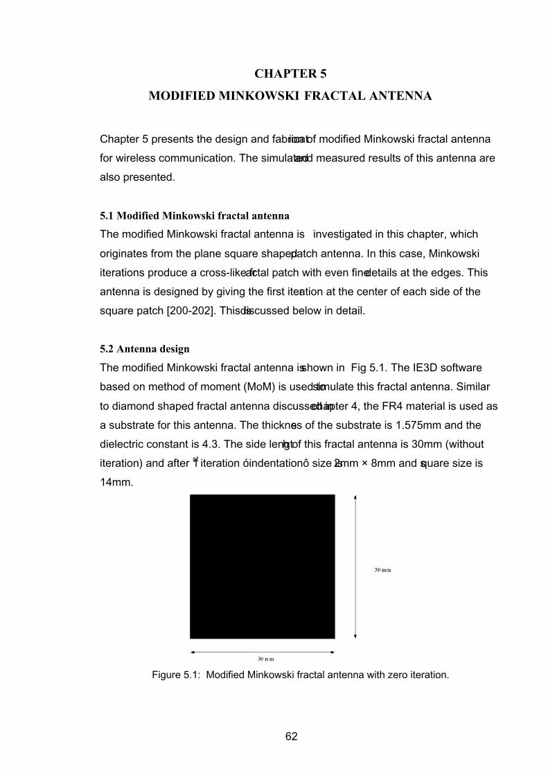
dielectric constant is 4.3. The side length of this fractal antenna is 30mm (without

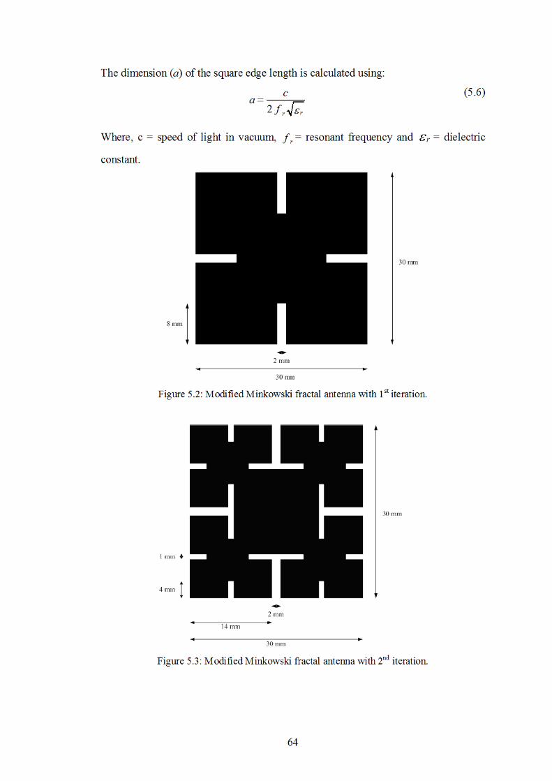
iteration) and after 1st�LWHUDWLRQ�µLQGHQWDWLRQ¶�VL]H�LV 2mm × 8mm and square size is

14mm.

Figure 5.1: Modified Minkowski fractal antenna with zero iteration.

62

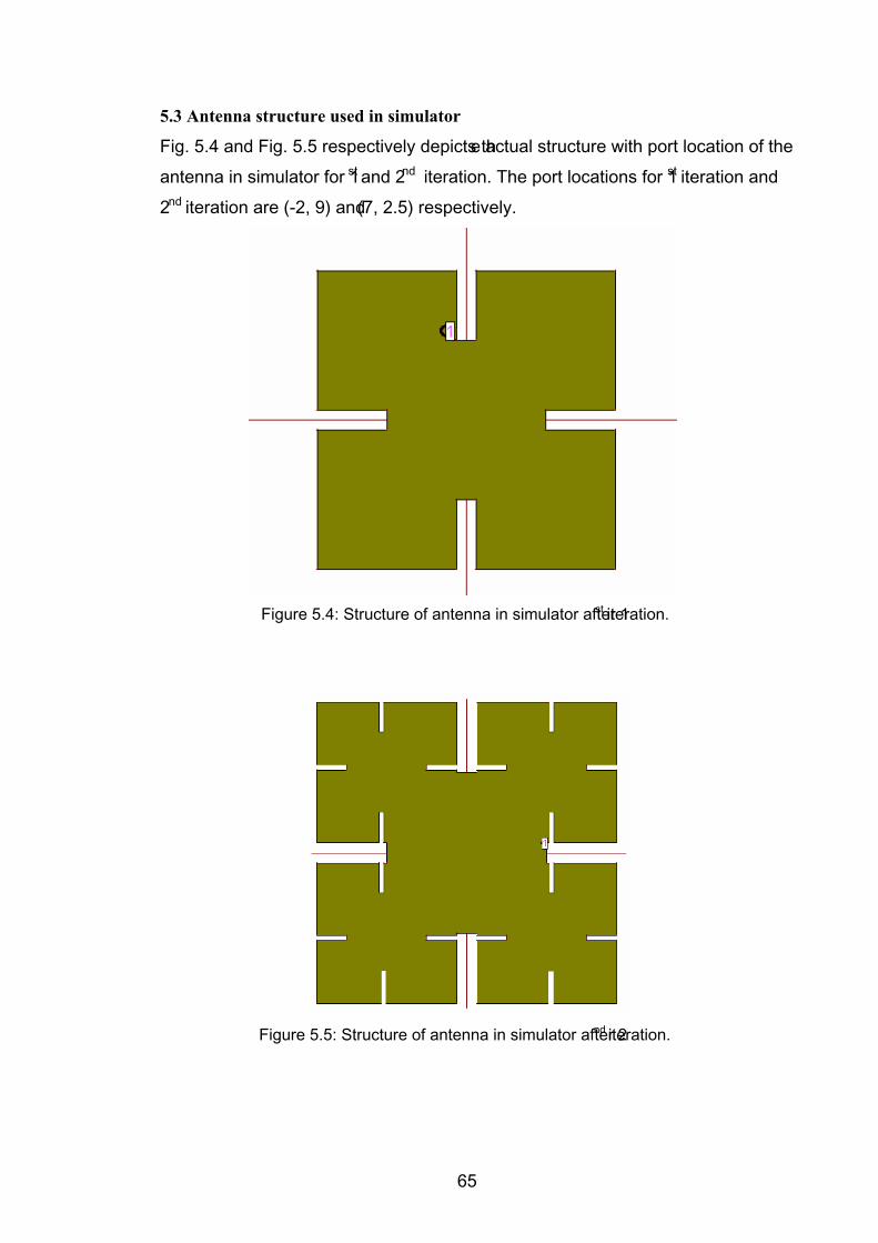
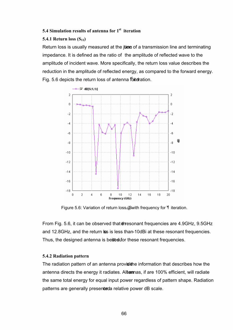
5.3 Antenna structure used in simulator

Fig. 5.4 and Fig. 5.5 respectively depicts the actual structure with port location of the

antenna in simulator for 1st and 2nd iteration. The port locations for 1st iteration and

2nd iteration are (-2, 9) and (7, 2.5) respectively.

Figure 5.4: Structure of antenna in simulator after 1st iteration.

Figure 5.5: Structure of antenna in simulator after 2nd iteration.

65

5.4 Simulation results of antenna for 1st iteration

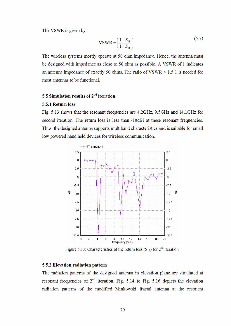
5.4.1 Return loss (S11)

Return loss is usually measured at the junction of a transmission line and terminating

impedance. It is defined as the ratio of the amplitude of reflected wave to the

amplitude of incident wave. More specifically, the return loss value describes the

reduction in the amplitude of reflected energy, as compared to the forward energy.

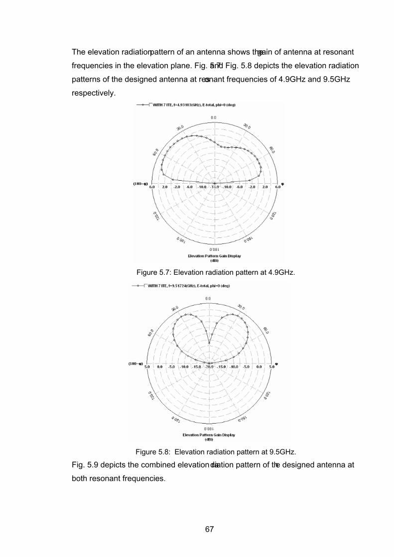
Fig. 5.6 depicts the return loss of antenna for 1st iteration.

Figure 5.6: Variation of return loss (S11) with frequency for 1st iteration.

From Fig. 5.6, it can be observed that the resonant frequencies are 4.9GHz, 9.5GHz

and 12.8GHz, and the return loss is less than -10dBi at these resonant frequencies.

Thus, the designed antenna is best suited for these resonant frequencies.

5.4.2 Radiation pattern

The radiation pattern of an antenna provides the information that describes how the

antenna directs the energy it radiates. All antennas, if are 100% efficient, will radiate

the same total energy for equal input power regardless of pattern shape. Radiation

patterns are generally presented on a relative power dB scale.

66

The elevation radiation pattern of an antenna shows the gain of antenna at resonant

frequencies in the elevation plane. Fig. 5.7 and Fig. 5.8 depicts the elevation radiation

patterns of the designed antenna at resonant frequencies of 4.9GHz and 9.5GHz

respectively.

Figure 5.7: Elevation radiation pattern at 4.9GHz.

Figure 5.8: Elevation radiation pattern at 9.5GHz.

Fig. 5.9 depicts the combined elevation radiation pattern of the designed antenna at

both resonant frequencies.

67

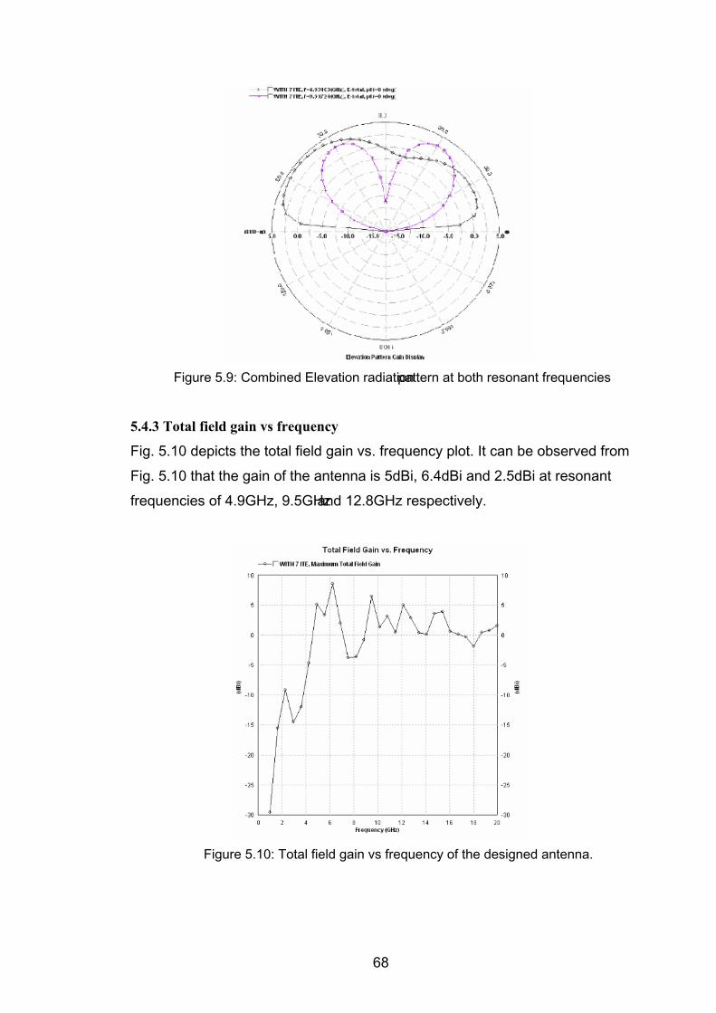
Figure 5.9: Combined Elevation radiation pattern at both resonant frequencies

5.4.3 Total field gain vs frequency

Fig. 5.10 depicts the total field gain vs. frequency plot. It can be observed from

Fig. 5.10 that the gain of the antenna is 5dBi, 6.4dBi and 2.5dBi at resonant

frequencies of 4.9GHz, 9.5GHz and 12.8GHz respectively.

Figure 5.10: Total field gain vs frequency of the designed antenna.

68

5.4.4 Directivity of the designed antenna

Fig. 5.11 depicts the directivity vs. frequency plot. The directivity of the designed

antenna obtained at resonant frequencies of 4.9GHz, 9.5GHz and 12.8GHz is 7.5dBi,

9.5dBi and 9.1dBi respectively.

Figure 5.11: Directivity vs frequency graph of the designed antenna.

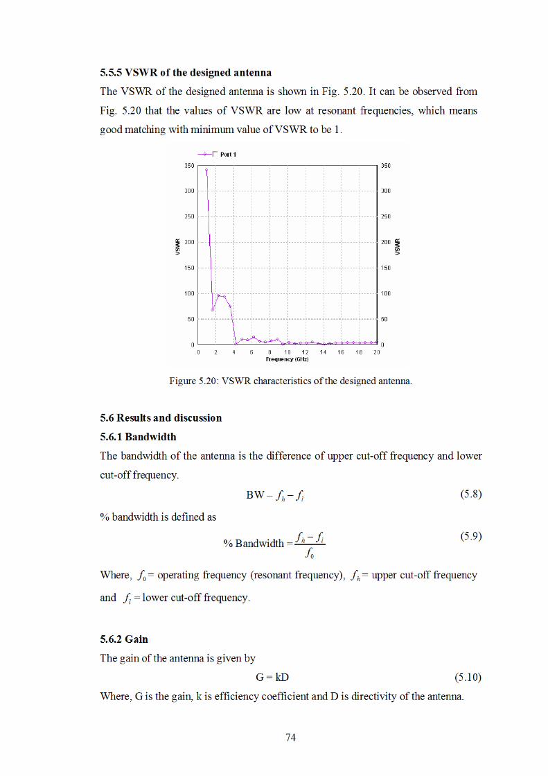
5.4.5 VSWR of the designed antenna

Fig. 5.12 shows the Voltage Standing Wave Ratio (VSWR) of the designed

antenna.VSWR is the ratio between the maximum voltage and minimum voltage

along transmission line.

Figure 5.12: VSWR characteristics of the designed antenna for 1st iteration.

69

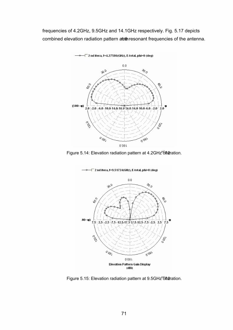
frequencies of 4.2GHz, 9.5GHz and 14.1GHz respectively. Fig. 5.17 depicts

combined elevation radiation pattern at three resonant frequencies of the antenna.

Figure 5.14: Elevation radiation pattern at 4.2GHz of 2nd iteration.

Figure 5.15: Elevation radiation pattern at 9.5GHz of 2nd iteration.

71

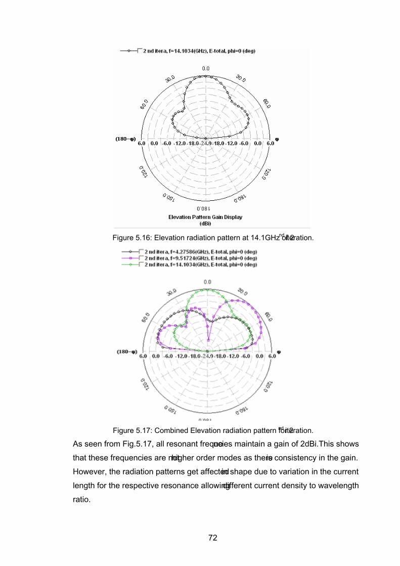
Figure 5.16: Elevation radiation pattern at 14.1GHz of 2nd iteration.

Figure 5.17: Combined Elevation radiation pattern for 2nd iteration.

As seen from Fig.5.17, all resonant frequencies maintain a gain of 2dBi.This shows

that these frequencies are not higher order modes as there is consistency in the gain.

However, the radiation patterns get affected in shape due to variation in the current

length for the respective resonance allowing different current density to wavelength

ratio.

72

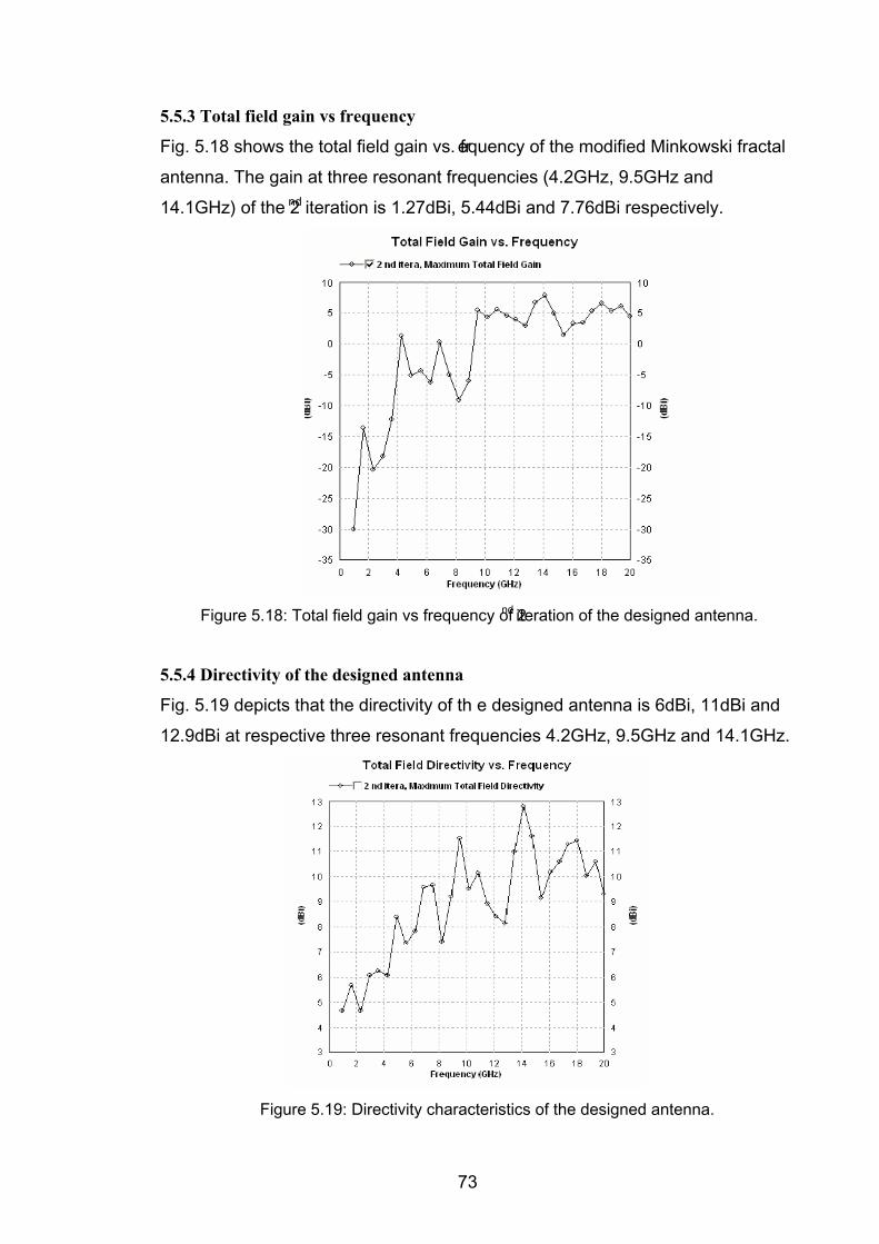
5.5.3 Total field gain vs frequency

Fig. 5.18 shows the total field gain vs. frequency of the modified Minkowski fractal

antenna. The gain at three resonant frequencies (4.2GHz, 9.5GHz and

14.1GHz) of the 2nd iteration is 1.27dBi, 5.44dBi and 7.76dBi respectively.

Figure 5.18: Total field gain vs frequency of 2nd iteration of the designed antenna.

5.5.4 Directivity of the designed antenna

Fig. 5.19 depicts that the directivity of th e designed antenna is 6dBi, 11dBi and

12.9dBi at respective three resonant frequencies 4.2GHz, 9.5GHz and 14.1GHz.

Figure 5.19: Directivity characteristics of the designed antenna.

73

The gain of the antenna at 14.1GHz is 7.76dBi and the dir ectivity is 12.9dBi.

Calculating the efficiency,

k = 7.76/12.9 = 0.6015 (5.28)

From the above results, the efficiency of the antenna at 14.1GHz is 60.15%.

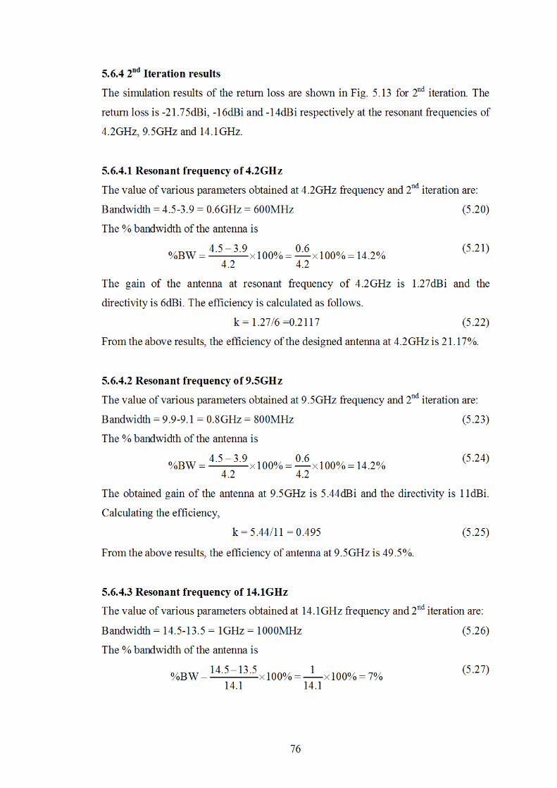
Table 5.1: Summary of 1st iteration results.

Resonant Frequency (GHz)

Return loss (dB)

Gain (dBi)

Directivity(dBi)

Bandwidth (MHz)

% Bandwidth

VSWR Efficiency Coefficient (k)

4.9 -14.4 5 7.5 500 10.2 1.33 0.666

9.5 -17.6 6.4 9.5 1000 10.5 1.2 0.673

12.8 -10.8 2.5 9.1 300 2.34 1.3 0.275

Table 5.2: Summary of 2nd iteration results.

Resonant

Frequency

(GHz)

Return

loss

Gain

(dBi)

Directivity

(dBi)

Bandwidth

�MHz��

%

Bandwidth

VSWR Efficiency

Coefficient

(k)

4.2 -21.75 1.27 6 600 14.2 1.6 0.2117

9.5 -16 5.44 11 800 14.2 1.5 0.495

14.1 -14 7.76 12.9 1000 7 1.40 0.6015

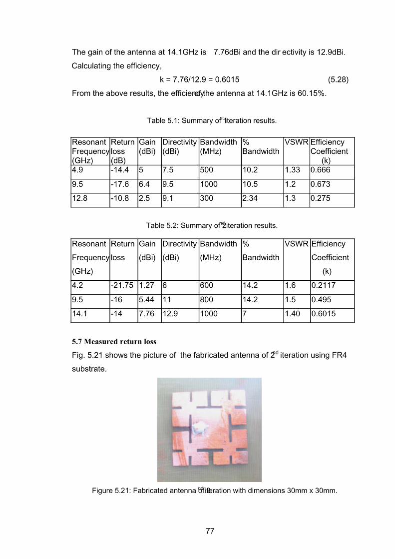
5.7 Measured return loss

Fig. 5.21 shows the picture of the fabricated antenna of 2nd iteration using FR4

substrate.

Figure 5.21: Fabricated antenna of 2nd iteration with dimensions 30mm x 30mm.

77

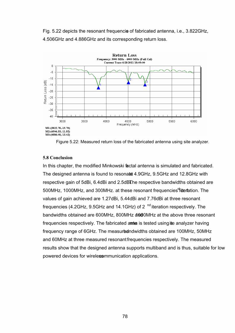
Fig. 5.22 depicts the resonant frequencies of fabricated antenna, i.e., 3.822GHz,

4.506GHz and 4.886GHz and its corresponding return loss.

Figure 5.22: Measured return loss of the fabricated antenna using site analyzer.

5.8 Conclusion

In this chapter, the modified Minkowski fractal antenna is simulated and fabricated.

The designed antenna is found to resonate at 4.9GHz, 9.5GHz and 12.8GHz with

respective gain of 5dBi, 6.4dBi and 2.5dBi. The respective bandwidths obtained are

500MHz, 1000MHz, and 300MHz. at these resonant frequencies for 1st iteration. The

values of gain achieved are 1.27dBi, 5.44dBi and 7.76dBi at three resonant

frequencies (4.2GHz, 9.5GHz and 14.1GHz) of 2 nd iteration respectively. The

bandwidths obtained are 600MHz, 800MHz and 1000MHz at the above three resonant

frequencies respectively. The fabricated antenna is tested using site analyzer having

frequency range of 6GHz. The measured bandwidths obtained are 100MHz, 50MHz

and 60MHz at three measured resonant frequencies respectively. The measured

results show that the designed antenna supports multiband and is thus, suitable for low

powered devices for wireless communication applications.

78