Embed Size (px)
Citation preview
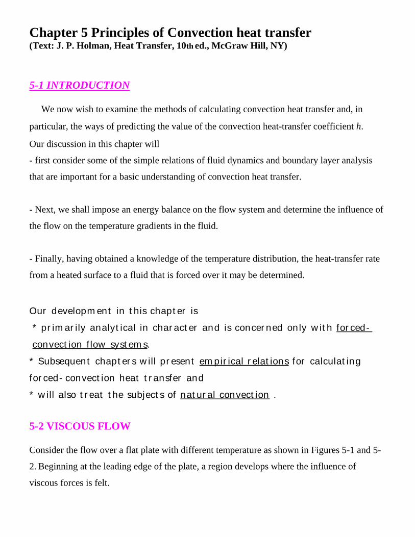
Chapter 5 Principles of Convection heat transfer (Text: J. P. Holman, Heat Transfer, 10th ed., McGraw Hill, NY)
5-1 INTRODUCTION We now wish to examine the methods of calculating convection heat transfer and, in
particular, the ways of predicting the value of the convection heat-transfer coefficient h.
Our discussion in this chapter will
- first consider some of the simple relations of fluid dynamics and boundary layer analysis
that are important for a basic understanding of convection heat transfer.
- Next, we shall impose an energy balance on the flow system and determine the influence of
the flow on the temperature gradients in the fluid.
- Finally, having obtained a knowledge of the temperature distribution, the heat-transfer rate
from a heated surface to a fluid that is forced over it may be determined.
Our development in this chapter is * primarily analytical in character and is concerned only with forced-convection flow systems. * Subsequent chapters will present empirical relations for calculating forced-convection heat transfer and * will also treat the subjects of natural convection . 5-2 VISCOUS FLOW Consider the flow over a flat plate with different temperature as shown in Figures 5-1 and 5-
2. Beginning at the leading edge of the plate, a region develops where the influence of
viscous forces is felt.
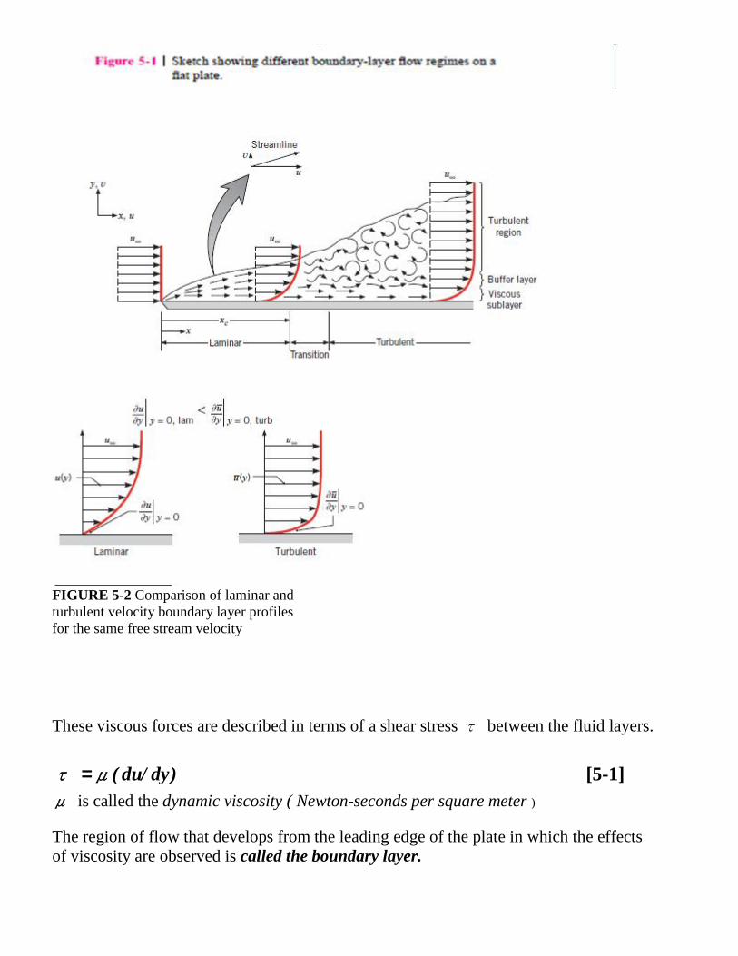
FIGURE 5-2 Comparison of laminar and turbulent velocity boundary layer profiles for the same free stream velocity These viscous forces are described in terms of a shear stress τ between the fluid layers.
τ =μ(du/dy) [5-1] μ is called the dynamic viscosity ( Newton-seconds per square meter )
The region of flow that develops from the leading edge of the plate in which the effects of viscosity are observed is called the boundary layer.
At the y position , where the velocity becomes %99 percent of the free-stream value, the boundary layer ends. The flow can be classified in the boundary layer to
• Initially laminar flow but at some critical distance from the leading edge, depending on the flow field and fluid properties, small disturbances in the
• flow begin to become amplified, and a transition process takes place until the flow becomes
• turbulent. The transition from laminar to turbulent flow occurs when u∞x/ν = ρu∞x/μ >5×10⁵ at flow on flat plate.
where u∞ = free-stream velocity, m/s x= distance from leading edge, m ν =μ/ρ = kinematic viscosity, m2/s This particular grouping of terms is called the Reynolds number, and is dimensionless if a consistent set of units is used for all the properties: Rex = u∞x/ν [5-2]
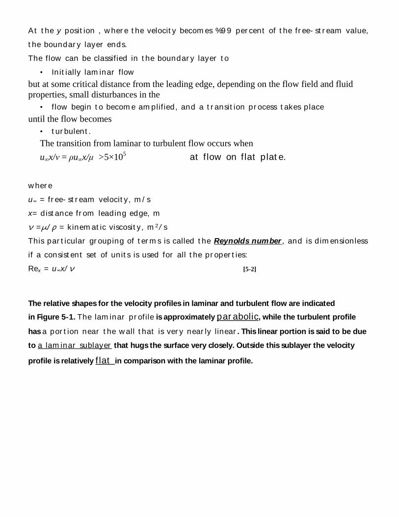
The relative shapes for the velocity profiles in laminar and turbulent flow are indicated
in Figure 5-1. The laminar profile is approximately parabolic, while the turbulent profile
has a portion near the wall that is very nearly linear. This linear portion is said to be due
to a laminar sublayer that hugs the surface very closely. Outside this sublayer the velocity
profile is relatively flat in comparison with the laminar profile.
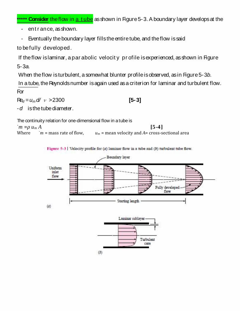
***** Consider the flow in a tube as shown in Figure 5-3. A boundary layer develops at the - entrance, as shown. - Eventually the boundary layer fills the entire tube, and the flow is said
to be fully developed. If the flow is laminar, a parabolic velocity profile is experienced, as shown in Figure 5-3a. When the flow is turbulent, a somewhat blunter profile is observed, as in Figure 5-3b. In a tube, the Reynolds number is again used as a criterion for laminar and turbulent flow. For Red = um d/ ν >2300 [5-3] -d is the tube diameter.
The continuity relation for one-dimensional flow in a tube is ˙m =ρ um A [5-4] Where ˙m = mass rate of flow, um = mean velocity and A= cross-sectional area
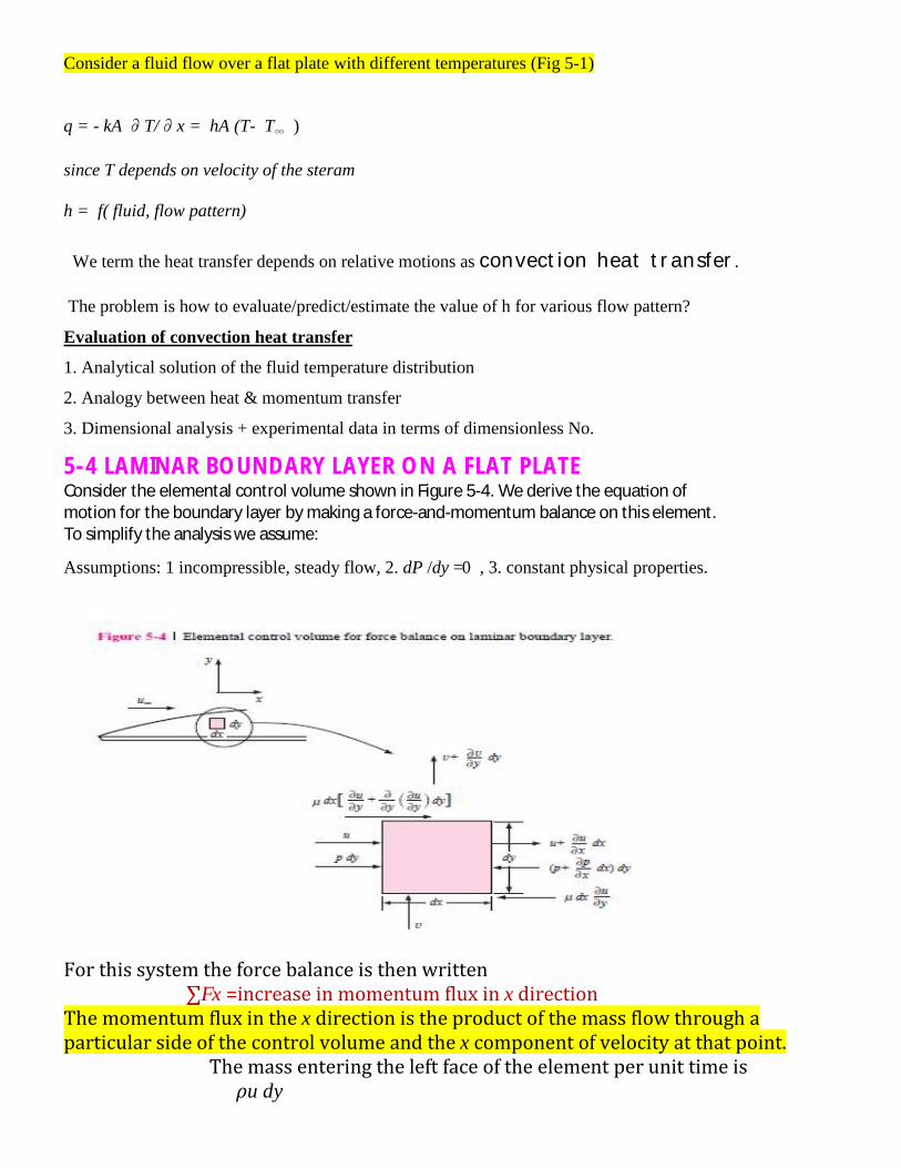
Consider a fluid flow over a flat plate with different temperatures (Fig 5-1)
q = - kA ∂T/∂x = hA (T- T∞ )
since T depends on velocity of the steram
h = f( fluid, flow pattern)
We term the heat transfer depends on relative motions as convection heat transfer.
The problem is how to evaluate/predict/estimate the value of h for various flow pattern?
Evaluation of convection heat transfer
1. Analytical solution of the fluid temperature distribution
2. Analogy between heat & momentum transfer
3. Dimensional analysis + experimental data in terms of dimensionless No.
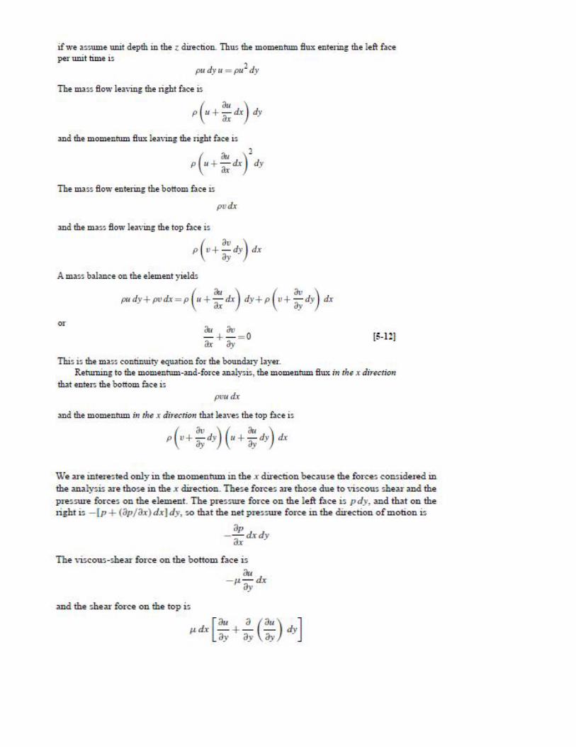
5-4 LAMINAR BOUNDARY LAYER ON A FLAT PLATE Consider the elemental control volume shown in Figure 5-4. We derive the equa on of motion for the boundary layer by making a force-and-momentum balance on this element. To simplify the analysis we assume:
Assumptions: 1 incompressible, steady flow, 2. dP /dy =0 , 3. constant physical properties.
For this system the force balance is then written ∑Fx =increase in momentum flux in x direction The momentum flux in the x direction is the product of the mass flow through a particular side of the control volume and the x component of velocity at that point. The mass entering the left face of the element per unit time is ρu dy
This is the momentum equation of the laminar boundary
layer with constant properties.
5-5 ENERGY EQUATION OF THE BOUNDARY LAYER C o n s e r v a t i o n o f E n e r g y Consider the elemental control volume shown in Figure 5-6. To simplify the analysis we assume 1. Incompressible steady flow
2. Constant viscosity, thermal conductivity, and specific heat
3. Negligible heat conduction in the direction of flow (x direction), i.e.,
∂T/∂x˂˂ ∂T/∂y
Then, for the element shown, the energy balance may be written
Energy convected in left face +energy convected in bottom face +heat conducted in bottom face +net viscous work done on element =energy convected out right face+energy convected out top face +heat conducted out top face
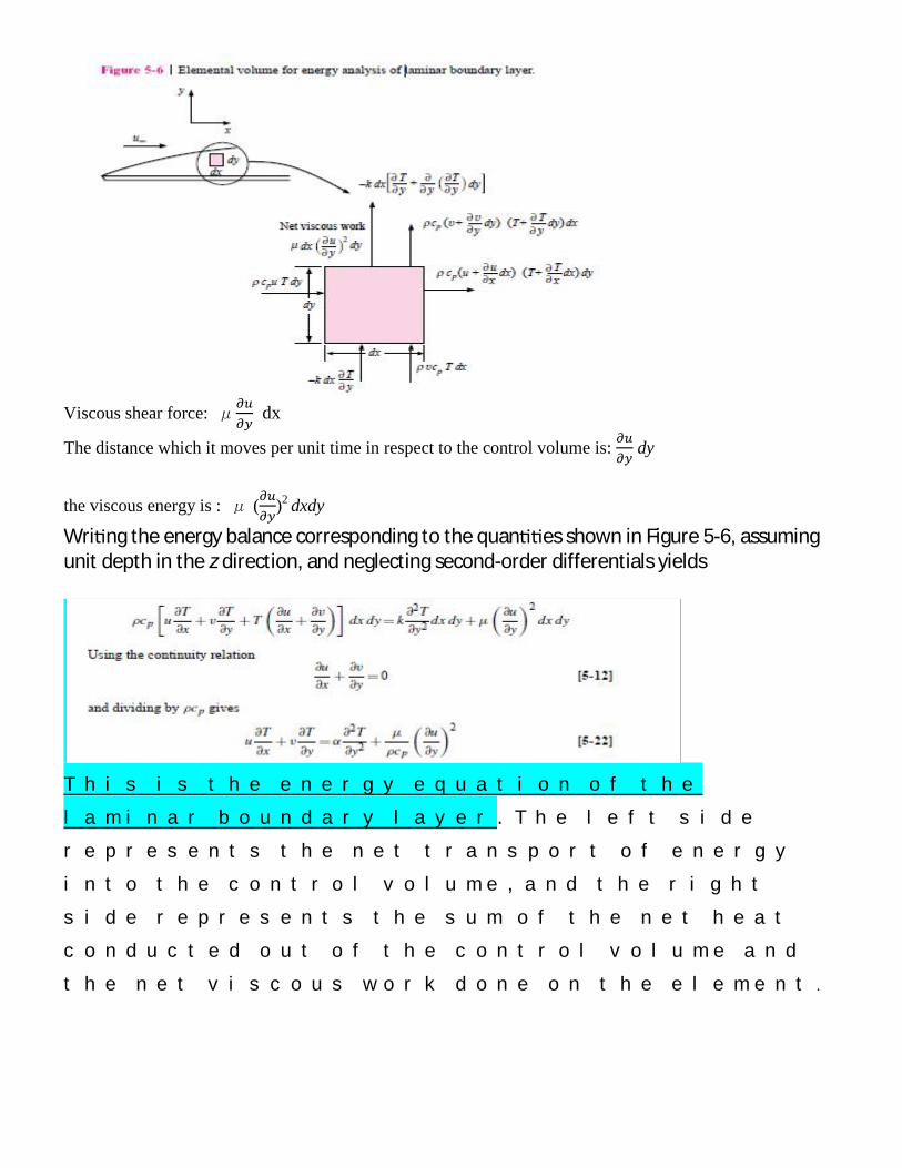
Viscous shear force: μ dx The distance which it moves per unit time in respect to the control volume is: dy
the viscous energy is : μ ( )2 dxdy
Wri ng the energy balance corresponding to the quan es shown in Figure 5-6, assuming unit depth in the z direction, and neglecting second-order differentials yields
T h i s i s t h e e n e r g y e q u a t i o n o f t h e
l a m i n a r b o u n d a r y l a y e r T h e. l e f t s i d e
r e p r e s e n t s t h e n e t t r a n s p o r t o f e n e r g y
i n t o t h e c o n t r o l v o l u m e a n d t h e r i g h t ,
s i d e r e p r e s e n t s t h e s u m o f t h e n e t h e a t
c o n d u c t e d o u t o f t h e c o n t r o l v o l u m e a n d
t h e n e t v i s c o u s w o r k d o n e o n t h e e l e m e n t .
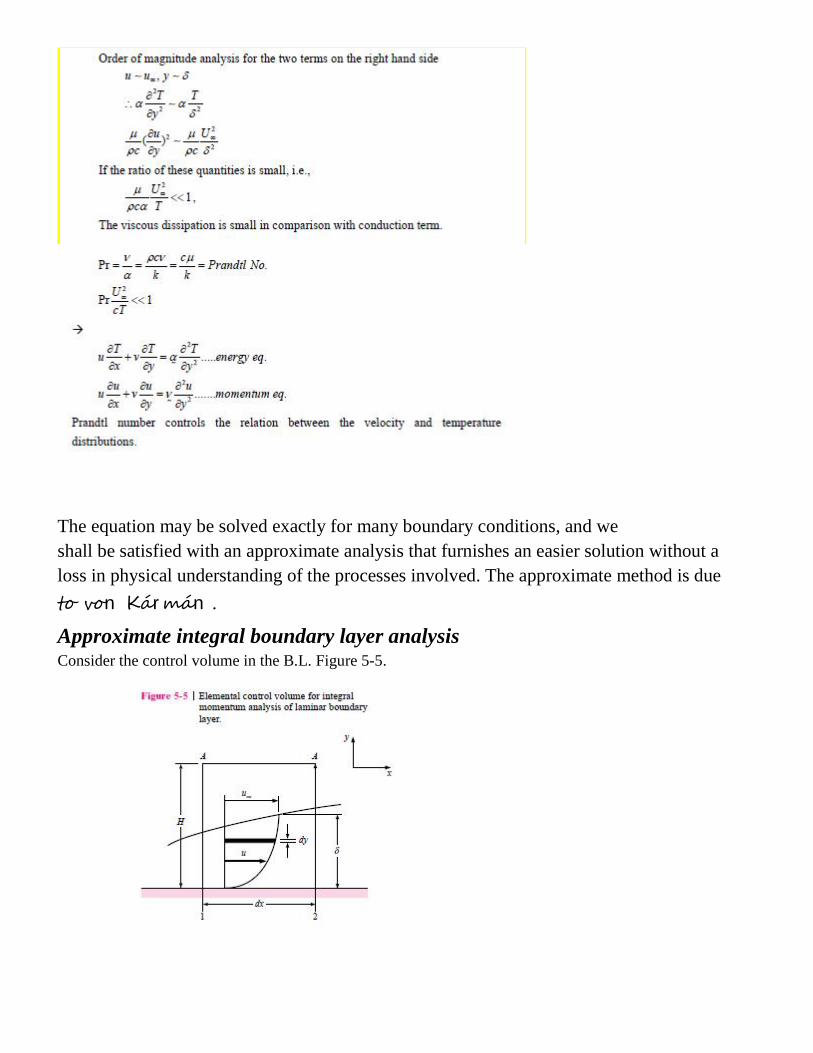
The equation may be solved exactly for many boundary conditions, and we shall be satisfied with an approximate analysis that furnishes an easier solution without a loss in physical understanding of the processes involved. The approximate method is due to von Kármán .
Approximate integral boundary layer analysis Consider the control volume in the B.L. Figure 5-5.
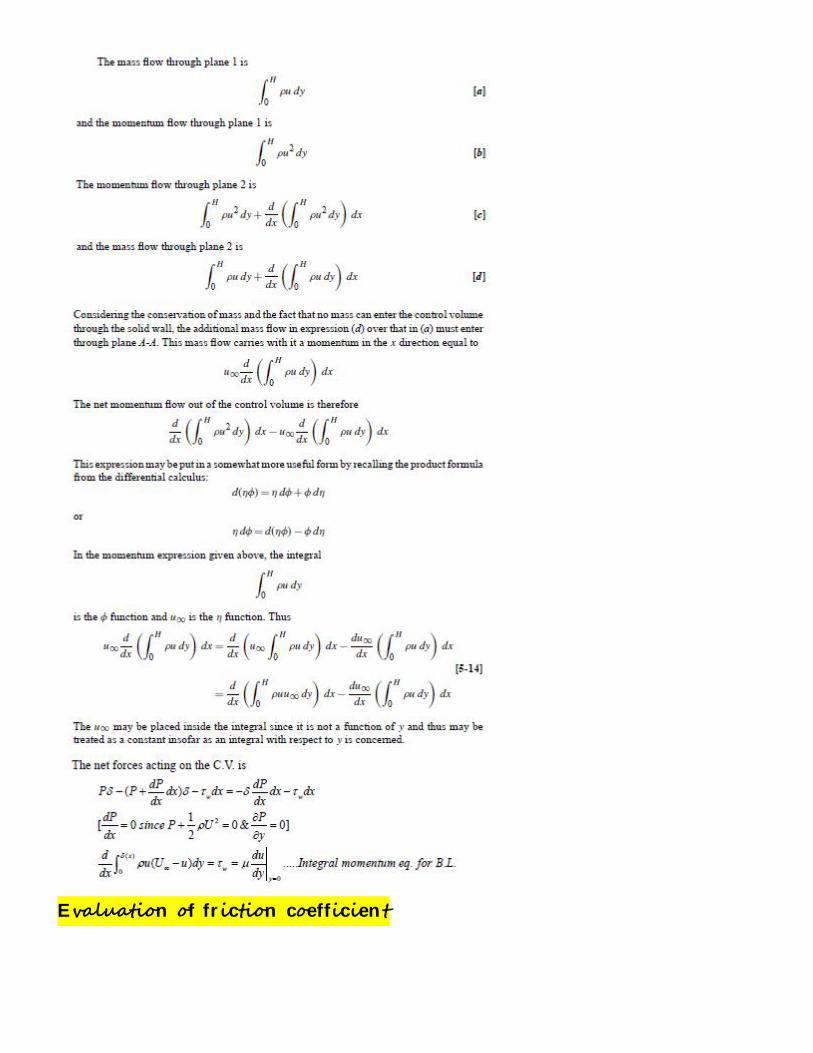
Evaluation of friction coefficient
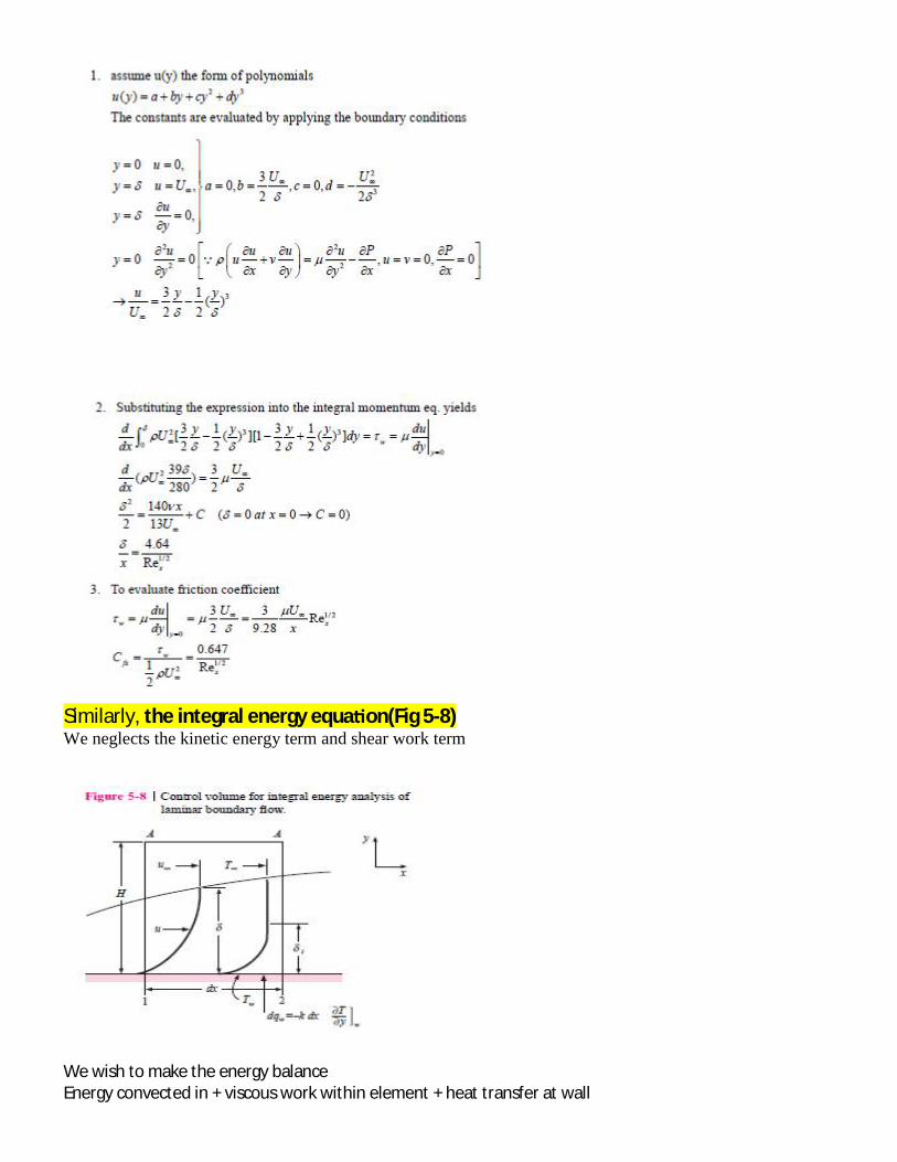
Similarly, the integral energy equa on(Fig 5-8) We neglects the kinetic energy term and shear work term
We wish to make the energy balance Energy convected in + viscous work within element + heat transfer at wall
=energy convected out [5-31] enthalpy enter across plane 1:∫ ( ) enthalpy leaves across plane 2:∫ ( ) + [∫ ( ) ] dx The enthalpy carried into the C. V. across the upper face is
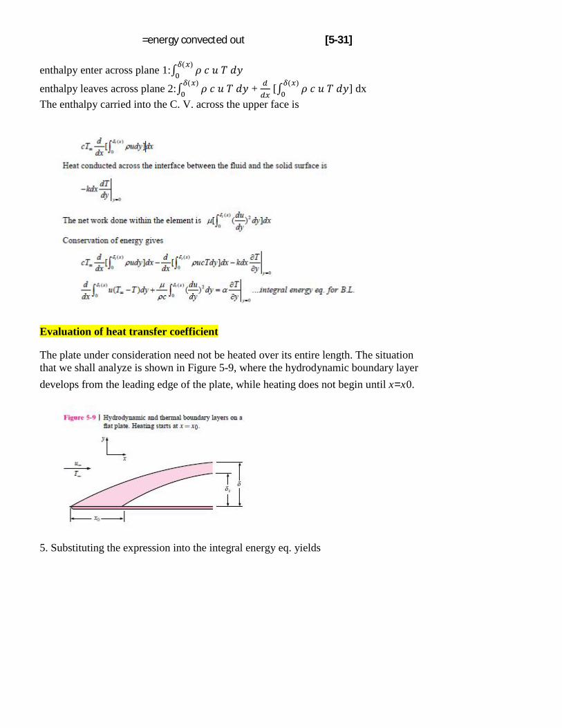
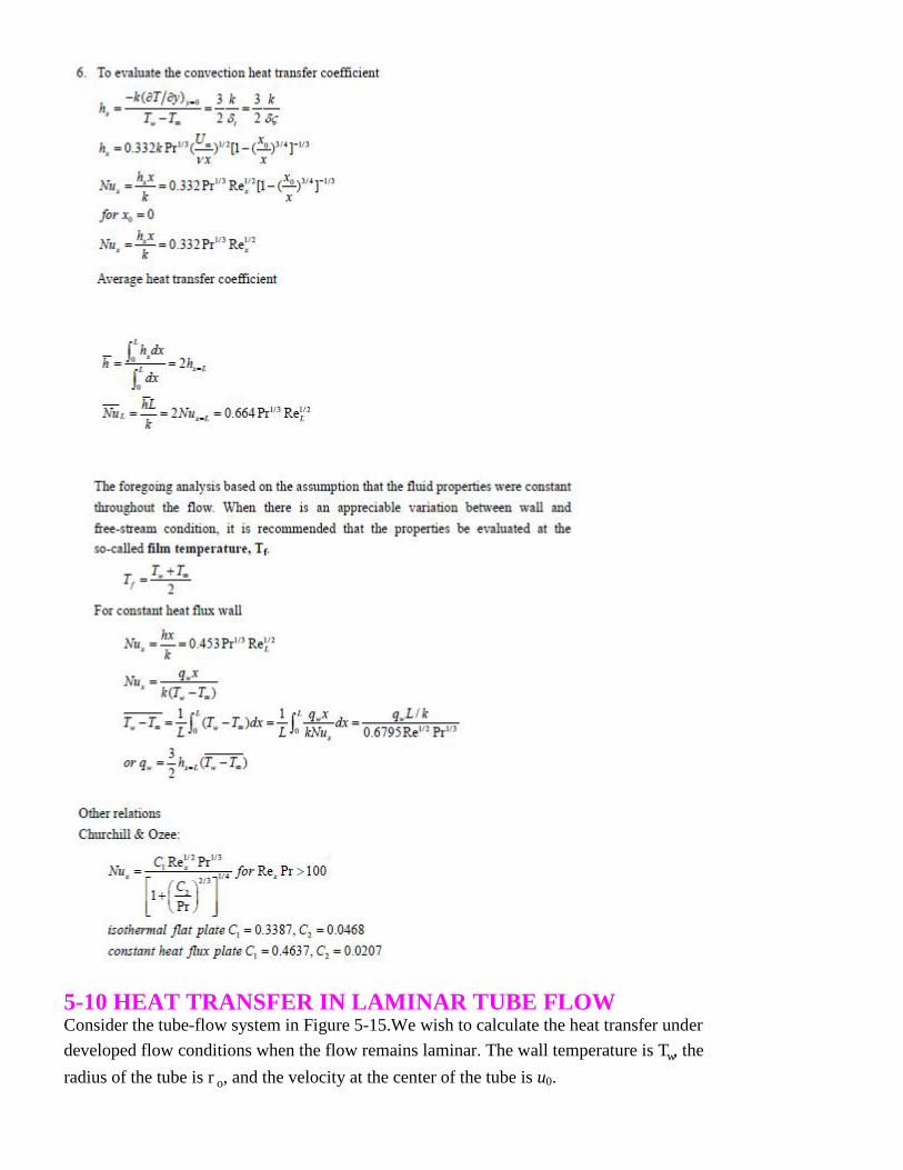
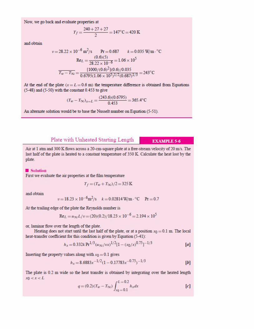
Evaluation of heat transfer coefficient The plate under consideration need not be heated over its entire length. The situation that we shall analyze is shown in Figure 5-9, where the hydrodynamic boundary layer develops from the leading edge of the plate, while heating does not begin until x=x0.
5. Substituting the expression into the integral energy eq. yields
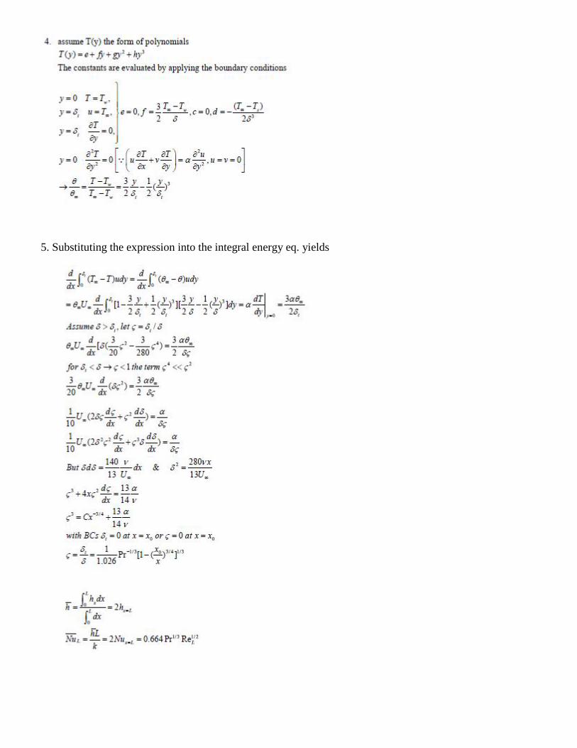
5. Substituting the expression into the integral energy eq. yields
5-10 HEAT TRANSFER IN LAMINAR TUBE FLOW Consider the tube-flow system in Figure 5-15.We wish to calculate the heat transfer under developed flow conditions when the flow remains laminar. The wall temperature is Tw, the radius of the tube is ro, and the velocity at the center of the tube is u0.
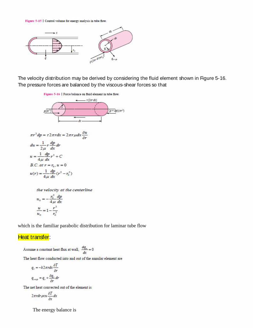
The velocity distribution may be derived by considering the fluid element shown in Figure 5-16. The pressure forces are balanced by the viscous-shear forces so that
which is the familiar parabolic distribution for laminar tube flow
Heat transfer:
The energy balance is
Net energy convected out=net heat conducted in
Neglecting second-order differentials, The energy balance gives
T h e b u l k t e m p e r a t u r e
L o c a l h e a t t r a n s f e r
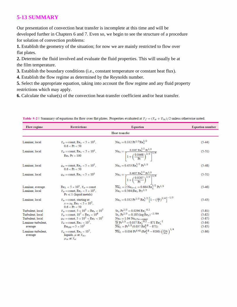
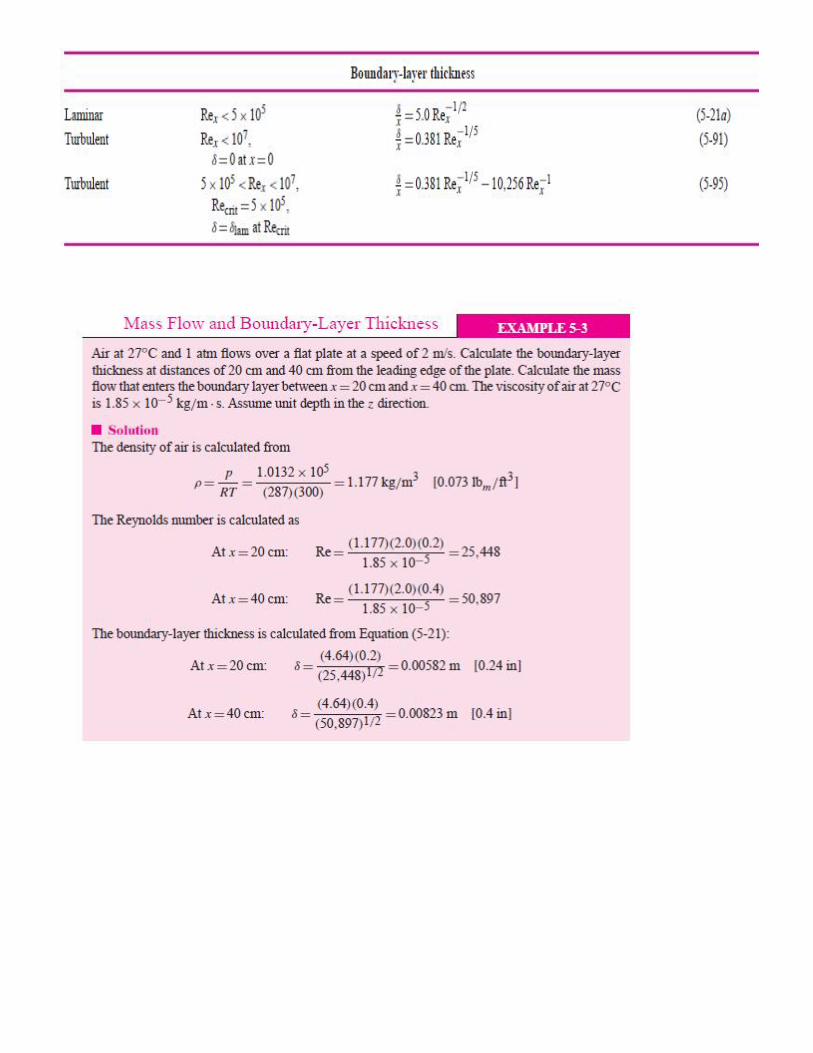
5-13 SUMMARY
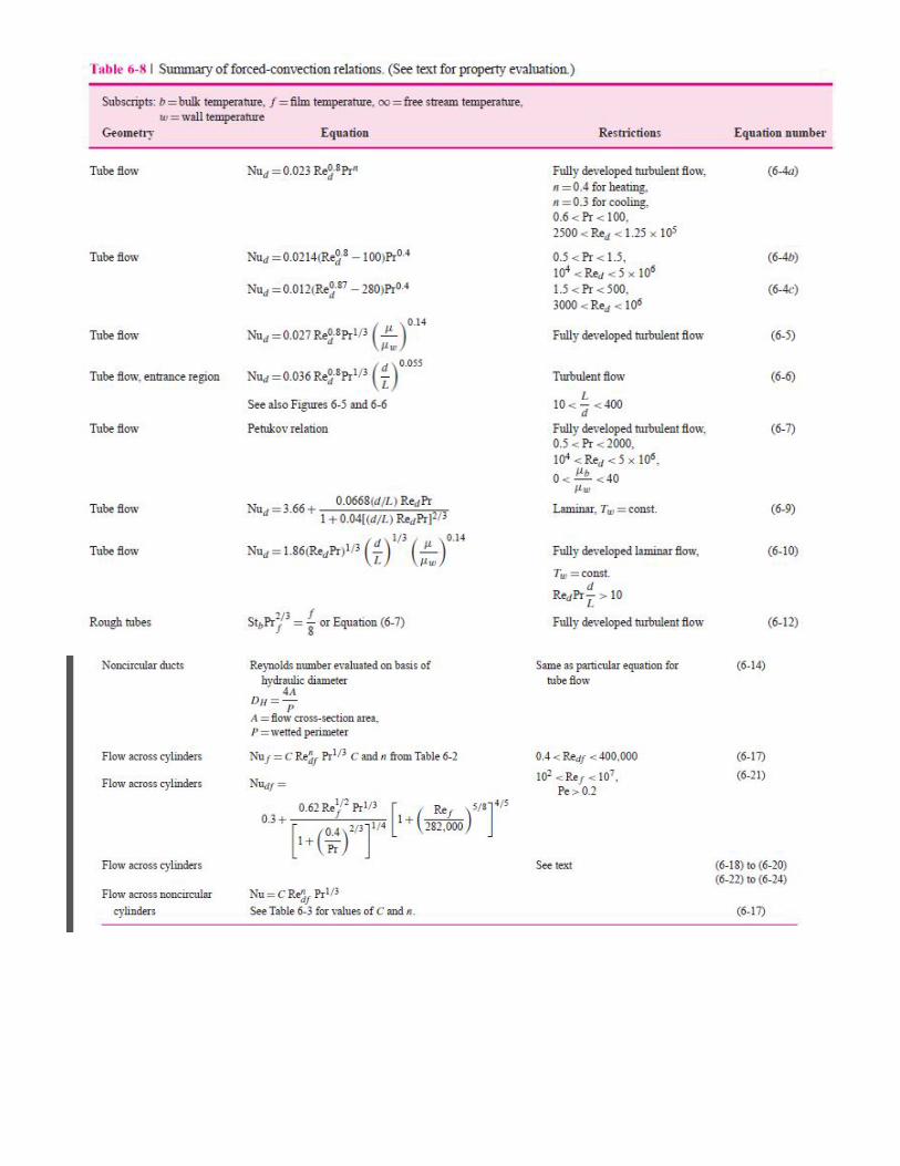
Our presentation of convection heat transfer is incomplete at this time and will be developed further in Chapters 6 and 7. Even so, we begin to see the structure of a procedure for solution of convection problems: 1. Establish the geometry of the situation; for now we are mainly restricted to flow over flat plates. 2. Determine the fluid involved and evaluate the fluid properties. This will usually be at the film temperature. 3. Establish the boundary conditions (i.e., constant temperature or constant heat flux). 4. Establish the flow regime as determined by the Reynolds number. 5. Select the appropriate equation, taking into account the flow regime and any fluid property restrictions which may apply. 6. Calculate the value(s) of the convection heat-transfer coefficient and/or heat transfer.
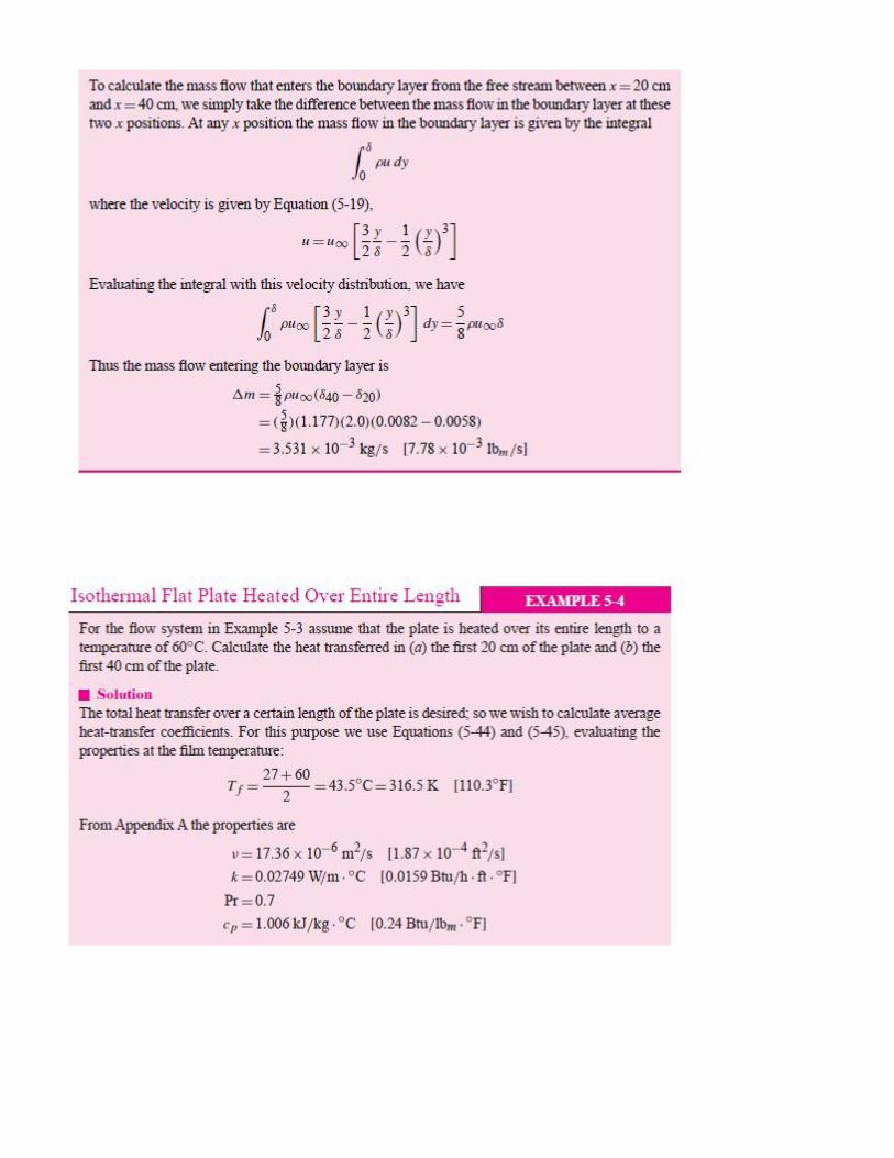
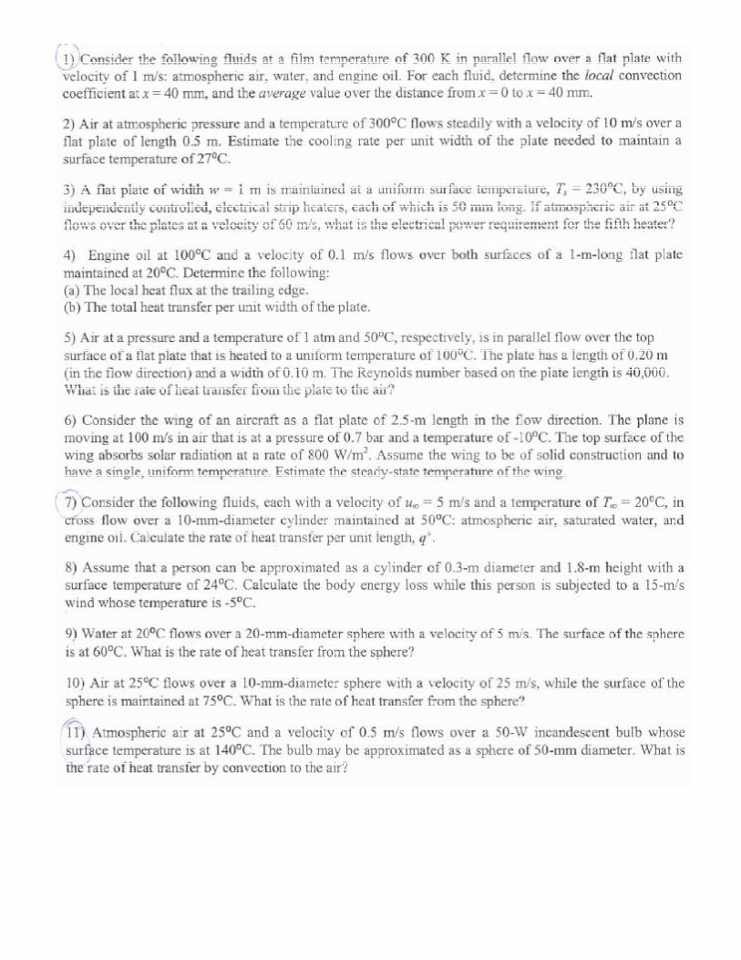
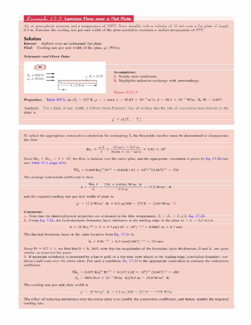
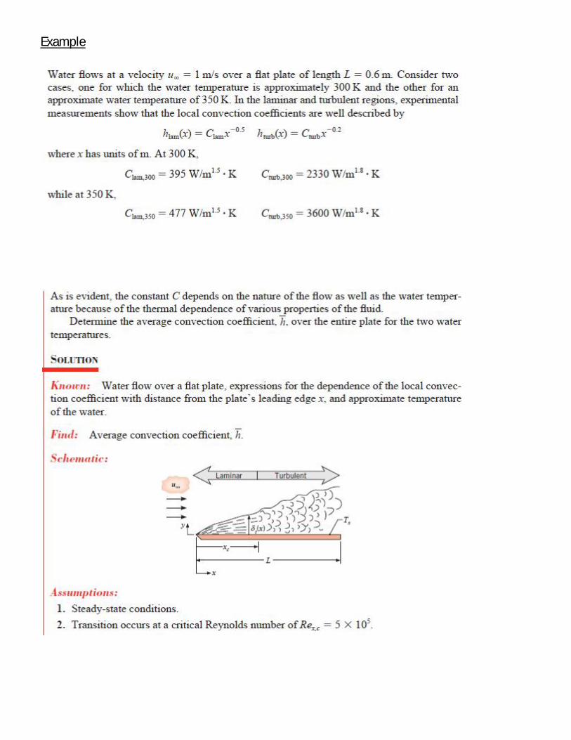
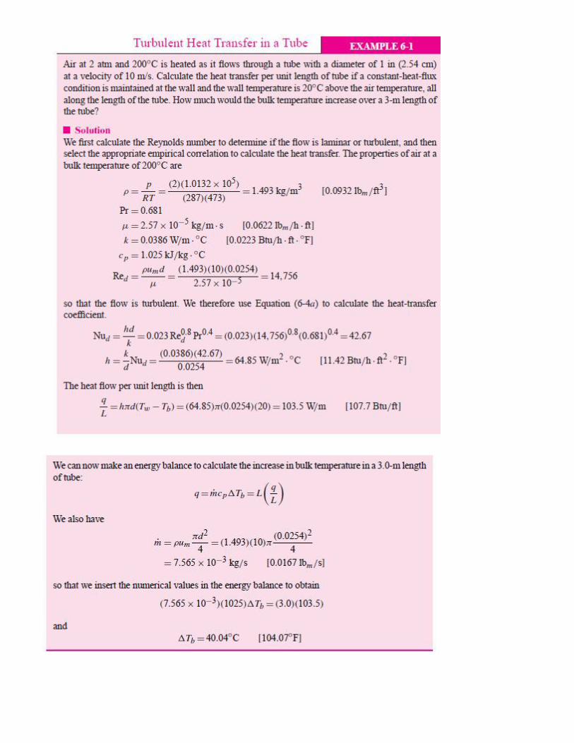
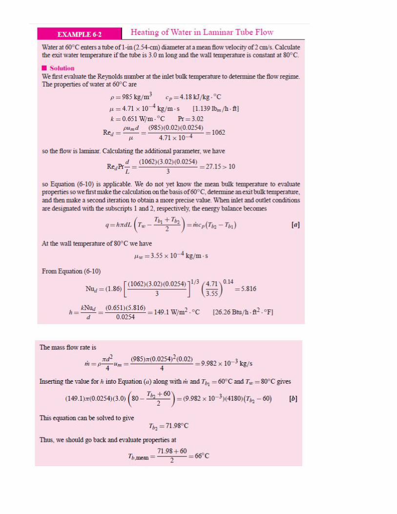
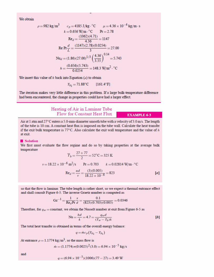
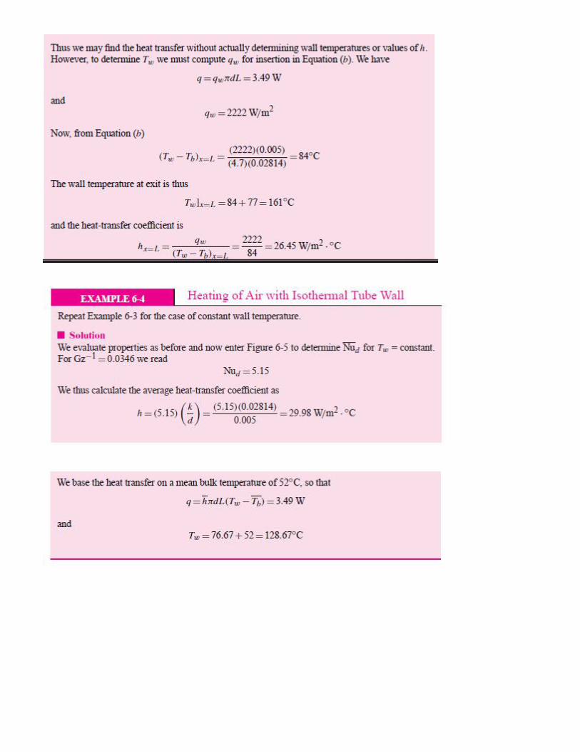
Example
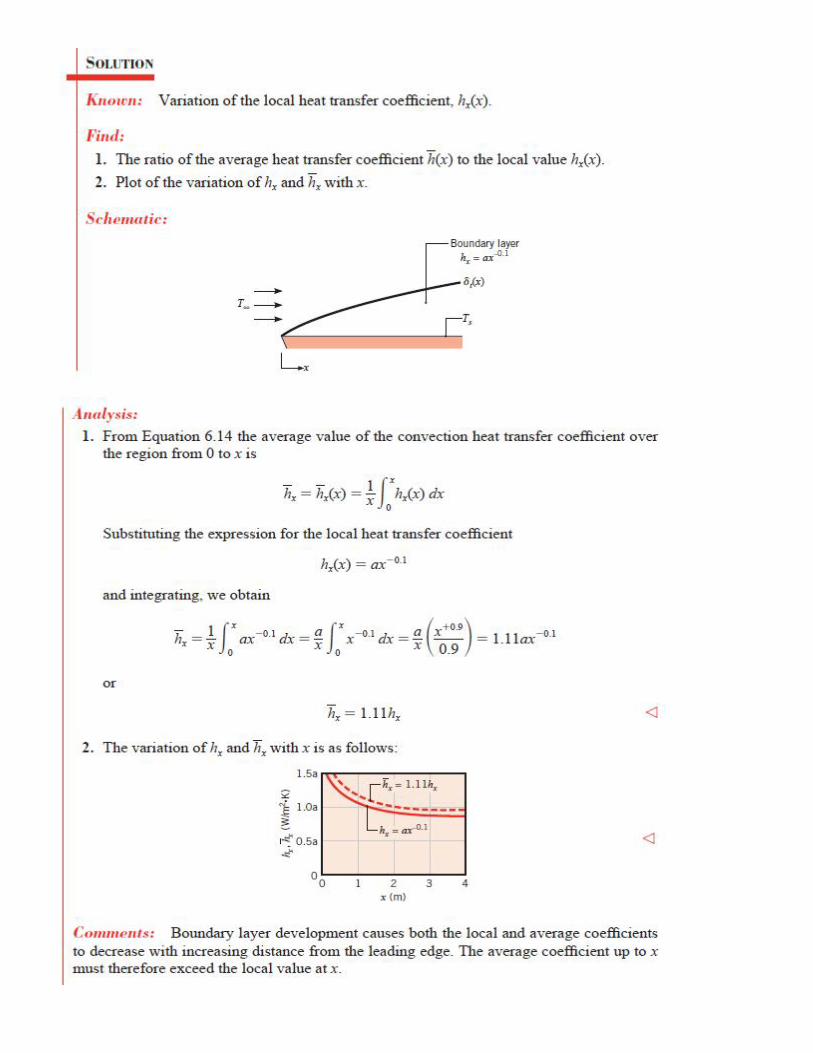
Example
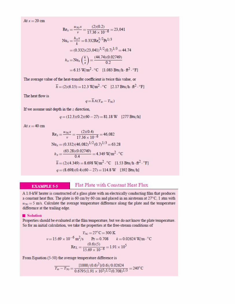
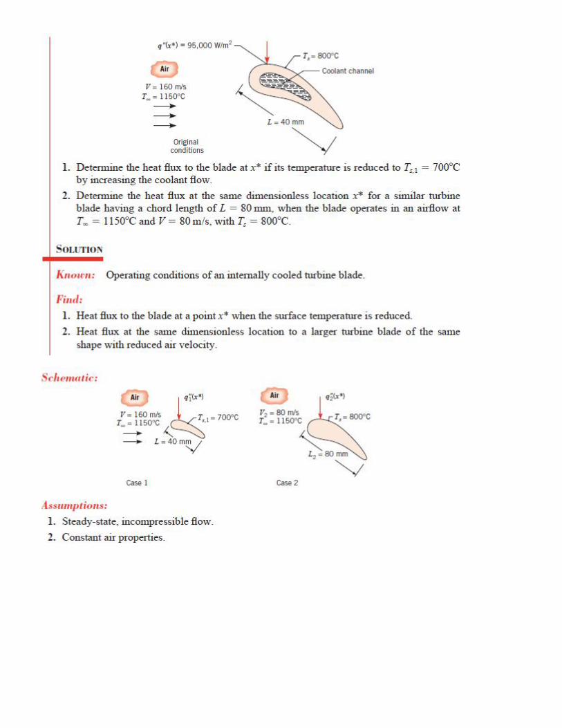
Example
Chapter 6
Empirical and Practical Relations for Forced – Convection Heat Transfer
Regrettably, it is not always possible to obtain analytical solutions to convection problems, and the individual is forced to resort to experimental methods to obtain design information, as well as to secure the more elusive data that increase the physical understanding of the heat-transfer processes.
6-2 EMPIRICAL RELATIONS FOR PIPE AND TUBE FLOW
In this section we present some of the more important and useful empirical relations and point out their limitations In Chapter 5 we noted that the bulk temperature represents energy average or “mixing cup” conditions. Thus, for the tube flow depicted in Figure 6-1 the total energy added can be expressed in terms of a bulk-temperature difference by
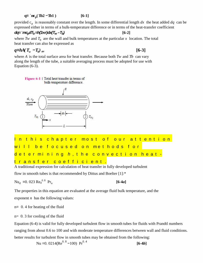
q= ˙mcp(Tb2 −Tb1 ) [6-1] provided cp is reasonably constant over the length. In some differential length dx the heat added dq can be expressed either in terms of a bulk-temperature difference or in terms of the heat-transfer coefficient dq= ˙mcpdTb =h(2πr)dx(Tw −Tb) [6-2] where Tw and Tb are the wall and bulk temperatures at the particular x location. The total heat transfer can also be expressed as
q=hA(Tw −Tb)av [6-3] where A is the total surface area for heat transfer. Because both Tw and Tb can vary along the length of the tube, a suitable averaging process must be adopted for use with Equation (6-3).
I n t h i s c h a p t e r m o s t o f o u r a t t e n t i o n
w i l l b e f o c u s e d o n m e t h o d s f o r
d e t e r m i n i n g h t h e c o n v e c t i o n h e a t, -
t r a n s f e r c o e f f i c i e n t . A traditional expression for calculation of heat transfer in fully developed turbulent
flow in smooth tubes is that recommended by Dittus and Boelter [1]:*
Nud =0.023 Red0.8 Prn [6-4a]
The properties in this equation are evaluated at the average fluid bulk temperature, and the
exponent n has the following values:
n= 0.4 for heating of the fluid
n= 0.3 for cooling of the fluid
Equation (6-4) is valid for fully developed turbulent flow in smooth tubes for fluids with Prandtl numbers
ranging from about 0.6 to 100 and with moderate temperature differences between wall and fluid conditions.
better results for turbulent flow in smooth tubes may be obtained from the following: Nu =0.0214(Re0.8 −100) Pr0.4 [6-4b]
for 0.5<Pr <1.5 and 104 <Re<5×10⁶ or
Nu =0.012( Re0.87 −280) Pr0.4 [6-4c] for 1.5<Pr <500 and 3000<Re<106
As described above, we may anticipate that the heat-transfer data will be dependent on the Reynolds and Prandtl numbers. A power function for each of these parameters is a simple type of relation to use, so we assume Nud =CRed
mPrn where C, m, and n are constants to be determined from the experimental data.
To take into account the property variations, Sieder and Tate [2] recommend the following relation: Nud =0.027 Red
0.8Pr1/3(μ/μw)0.14 [6-5]
All properties are evaluated at bulk-temperature conditions, except μw, which is evaluated at the wall temperature. Equations (6-4) and (6-5) apply to fully developed turbulent flow in tubes. In the entrance region the flow is not developed, and Nusselt [3] recommended the following equation: Nud =0.036 Red
0.8 Pr1/3(d/L)0.055 for 10< L/d <400 [6-6] where L is the length of the tube and d is the tube diameter. The properties in Equation (6-6) are evaluated at the mean bulk temperature.
If the channel through which the fluid flows is not of circular cross section, it is recommended that the heat-transfer correlations be based on the hydraulic diameter DH, defined by
DH = 4A/P [6-14] where A is the cross-sectional area of the flow and P is the wetted perimeter.
The hydraulic diameter should be used in calculating the Nusselt and Reynolds numbers.
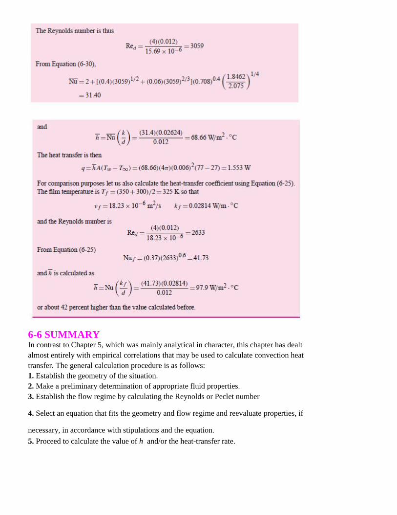
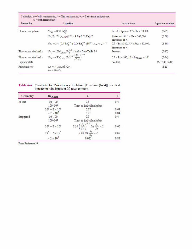
6-6 SUMMARY In contrast to Chapter 5, which was mainly analytical in character, this chapter has dealt almost entirely with empirical correlations that may be used to calculate convection heat transfer. The general calculation procedure is as follows: 1. Establish the geometry of the situation. 2. Make a preliminary determination of appropriate fluid properties. 3. Establish the flow regime by calculating the Reynolds or Peclet number 4. Select an equation that fits the geometry and flow regime and reevaluate properties, if necessary, in accordance with stipulations and the equation. 5. Proceed to calculate the value of h and/or the heat-transfer rate.