CHAPTER 5leeds-faculty.colorado.edu/.../FNCE4030-Fall-2012-ch05-handouts.pdfINVESTMENTS | BODIE, KANE, MARCUS 5-2 Interest Rate Determinants • Supply –Households • Demand –Businesses

INVESTMENTS | BODIE, KANE, MARCUS

Copyright © 2011 by The McGraw-Hill Companies, Inc. All rights reserved. McGraw-Hill/Irwin

CHAPTER 5

Introduction to Risk, Return, and

the Historical Record


5-2

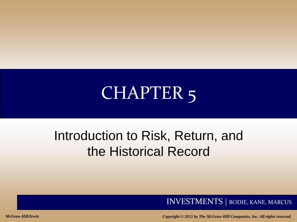
Interest Rate Determinants

• Supply

– Households

• Demand

– Businesses

• Government’s Net Supply and/or

Demand

– Federal Reserve Actions


5-3

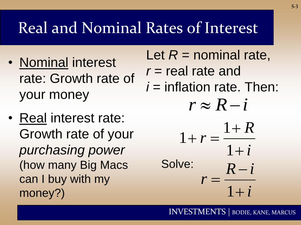
Real and Nominal Rates of Interest

• Nominal interest

rate: Growth rate of

your money

• Real interest rate:

Growth rate of your

purchasing power (how many Big Macs

can I buy with my

money?)

Let R = nominal rate,

r = real rate and

i = inflation rate. Then:

iRr

i

Rr

1

11

i

iRr

1

Solve:


5-4

Equilibrium Real Rate of Interest

• Determined by:

–Supply

–Demand

–Government actions

–Expected rate of inflation


5-5

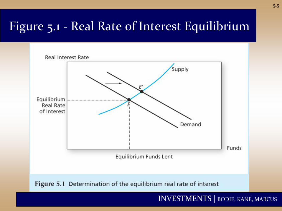
Figure 5.1 - Real Rate of Interest Equilibrium


5-6

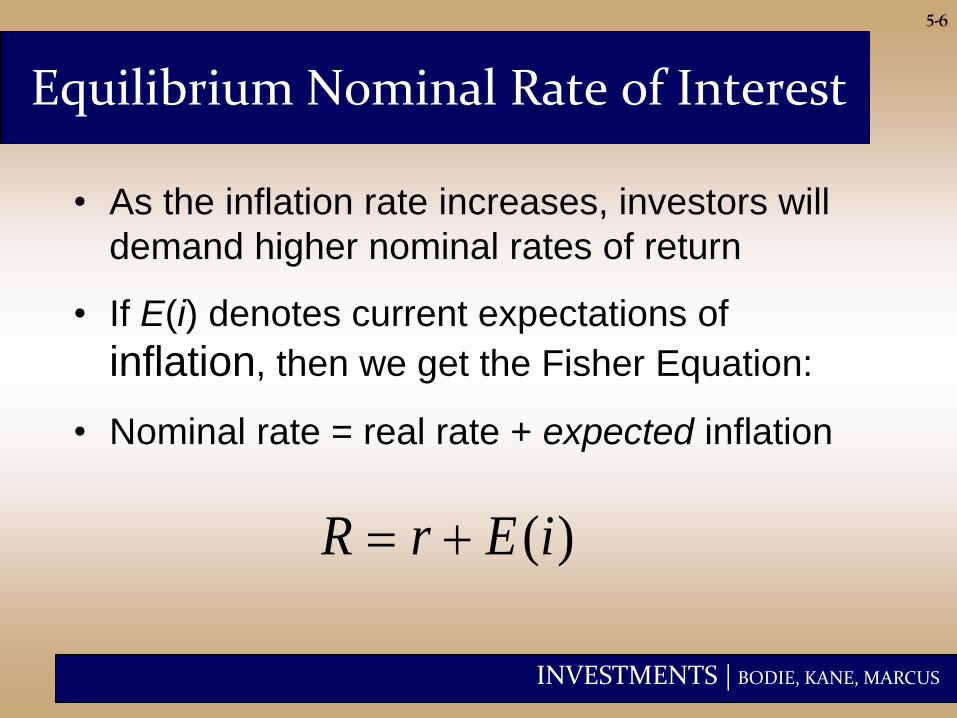
Equilibrium Nominal Rate of Interest

• As the inflation rate increases, investors will

demand higher nominal rates of return

• If E(i) denotes current expectations of

inflation, then we get the Fisher Equation:

• Nominal rate = real rate + expected inflation

( )R r E i


5-7

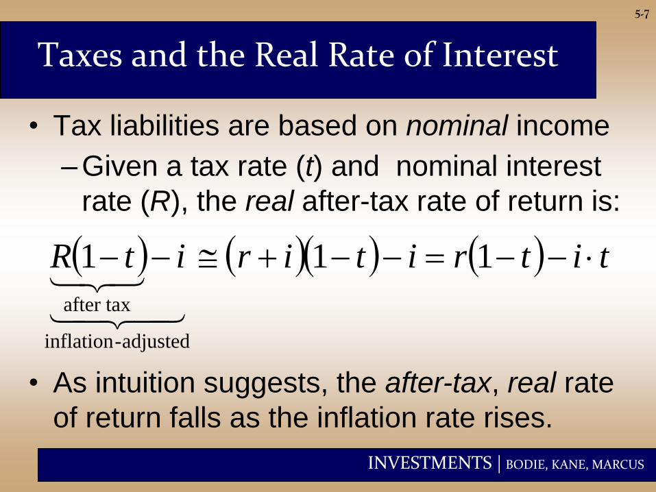
Taxes and the Real Rate of Interest

• Tax liabilities are based on nominal income

– Given a tax rate (t) and nominal interest

rate (R), the real after-tax rate of return is:

titritiritR 111

adjusted-inflation

after tax

• As intuition suggests, the after-tax, real rate

of return falls as the inflation rate rises.


5-8

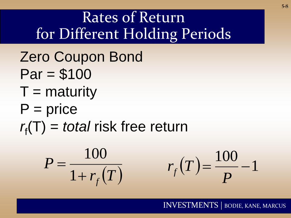
Rates of Return for Different Holding Periods

Zero Coupon Bond

Par = $100

T = maturity

P = price

rf(T) = total risk free return

TrP

f

1

100 1

100

PTrf


5-9

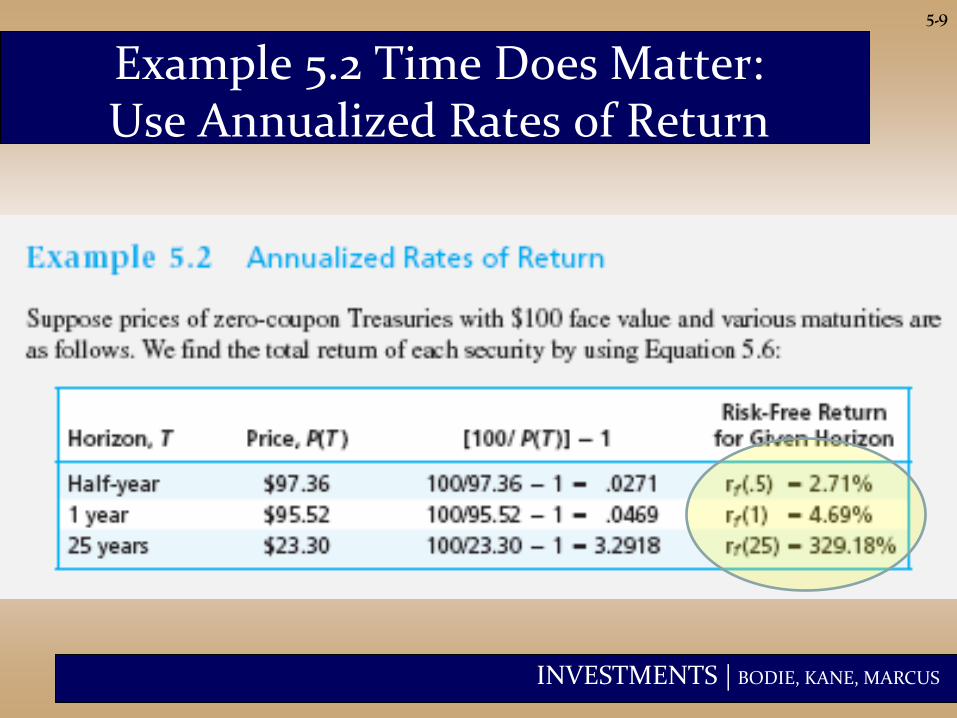
Example 5.2 Time Does Matter: Use Annualized Rates of Return


5-10

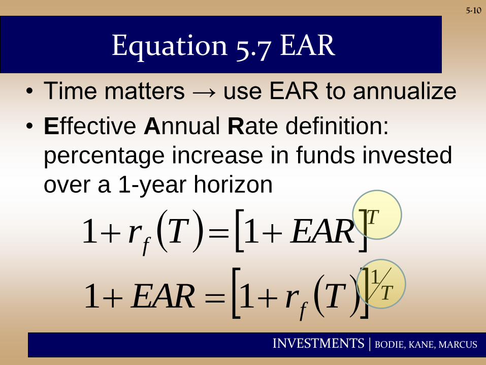
Equation 5.7 EAR

• Time matters → use EAR to annualize

• Effective Annual Rate definition:

percentage increase in funds invested

over a 1-year horizon

Tf EARTr 11

Tf TrEAR

1

11


5-11

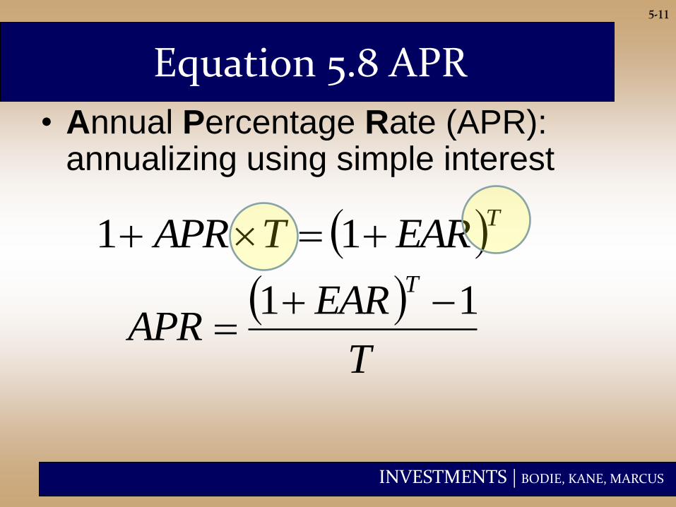
Equation 5.8 APR

• Annual Percentage Rate (APR): annualizing using simple interest

TEARTAPR 11

T

EARAPR

T11


5-12

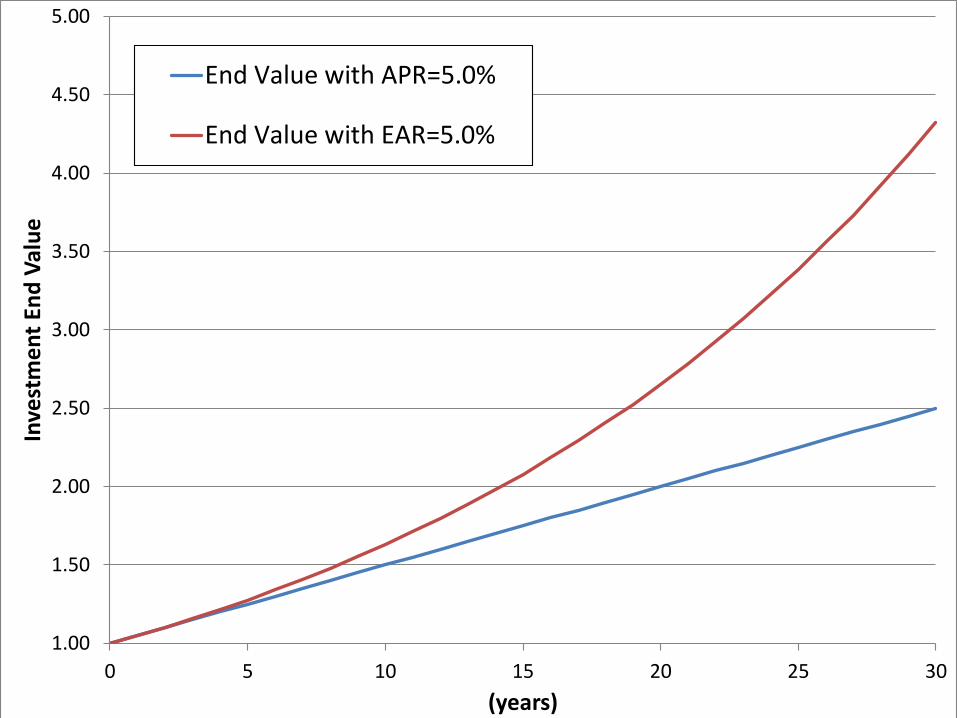
1.00

1.50

2.00

2.50

3.00

3.50

4.00

4.50

5.00

0 5 10 15 20 25 30

Inve

stm

en

t En

d V

alu

e

(years)

End Value with APR=5.0%

End Value with EAR=5.0%


5-13

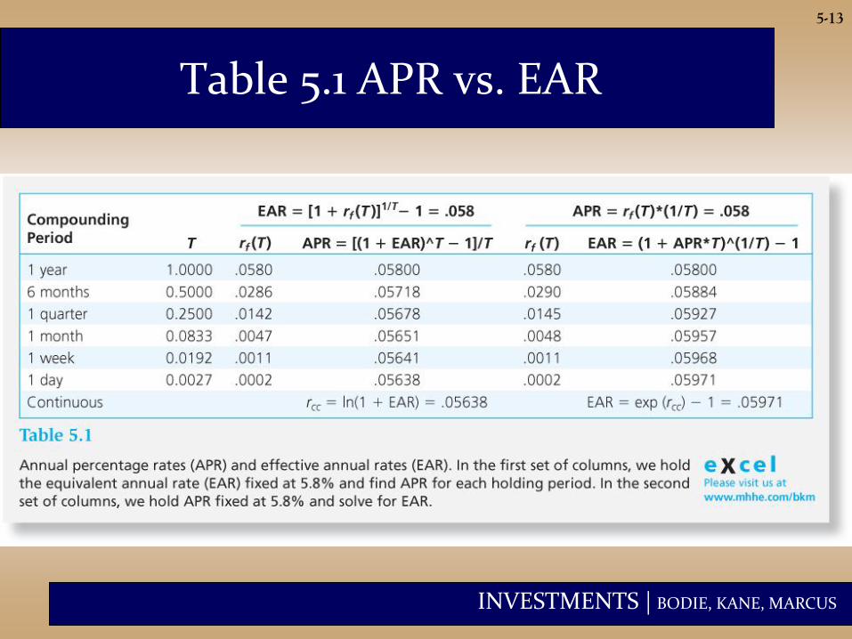
Table 5.1 APR vs. EAR


5-14

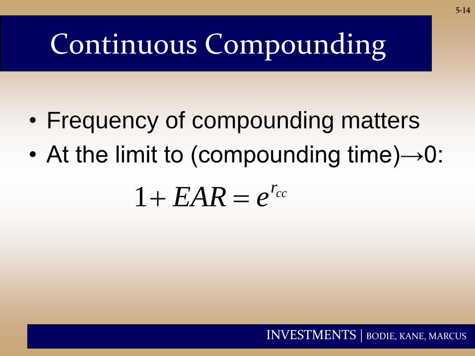
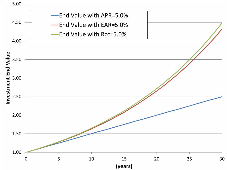
Continuous Compounding

• Frequency of compounding matters

• At the limit to (compounding time)→0:

ccreEAR 1


5-15

1.00

1.50

2.00

2.50

3.00

3.50

4.00

4.50

5.00

0 5 10 15 20 25 30

Inve

stm

en

t En

d V

alu

e

(years)

End Value with APR=5.0%

End Value with EAR=5.0%

End Value with Rcc=5.0%


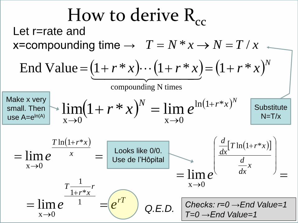
S

xTNxNT /* Let r=rate and

x=compounding time →

Nxrxrxr *1*1*1 Value End

timesN gcompoundin

NxrNexr *1ln

0x0x lim*1lim

How to derive Rcc

Substitute

N=T/x

x

xrT

e

*1ln

0xlim

xdx

d

xrTdx

d

e

*1ln

0xlim

rT

rxr

T

ee

1

*1

1

0xlim

Looks like 0/0.

Use de l’Hôpital

Q.E.D.

Make x very

small. Then

use A=eln(A)

Checks: r=0 →End Value=1

T=0 →End Value=1


5-17

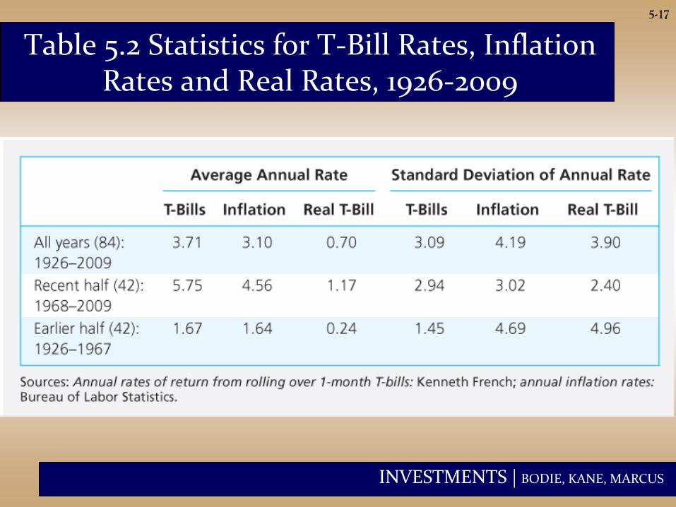
Table 5.2 Statistics for T-Bill Rates, Inflation Rates and Real Rates, 1926-2009


5-18

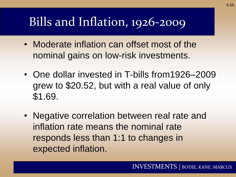
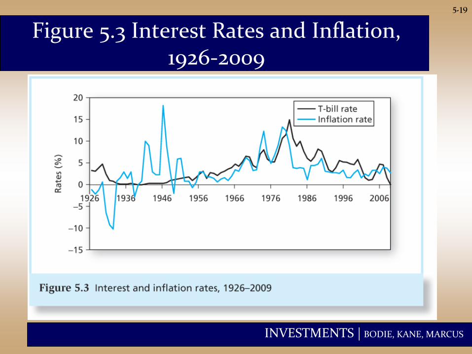
Bills and Inflation, 1926-2009

• Moderate inflation can offset most of the

nominal gains on low-risk investments.

• One dollar invested in T-bills from1926–2009

grew to $20.52, but with a real value of only

$1.69.

• Negative correlation between real rate and

inflation rate means the nominal rate

responds less than 1:1 to changes in

expected inflation.


5-19

Figure 5.3 Interest Rates and Inflation, 1926-2009


5-20

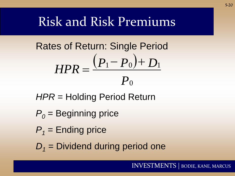
Risk and Risk Premiums

P

DPPHPR

0

101

HPR = Holding Period Return

P0 = Beginning price

P1 = Ending price

D1 = Dividend during period one

Rates of Return: Single Period


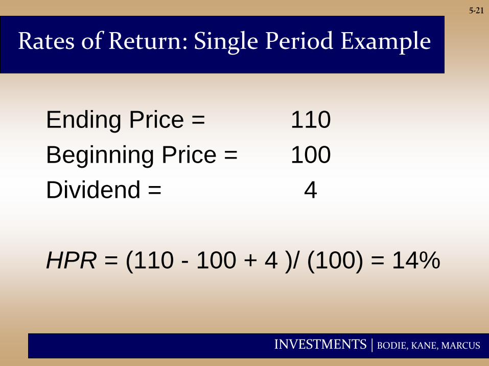
5-21

Ending Price = 110

Beginning Price = 100

Dividend = 4

HPR = (110 - 100 + 4 )/ (100) = 14%

Rates of Return: Single Period Example


5-22

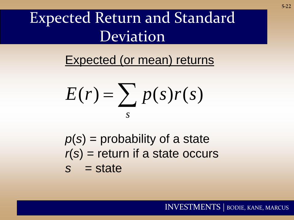
Expected (or mean) returns

p(s) = probability of a state

r(s) = return if a state occurs

s = state

Expected Return and Standard Deviation

( ) ( ) ( )s

E r p s r s


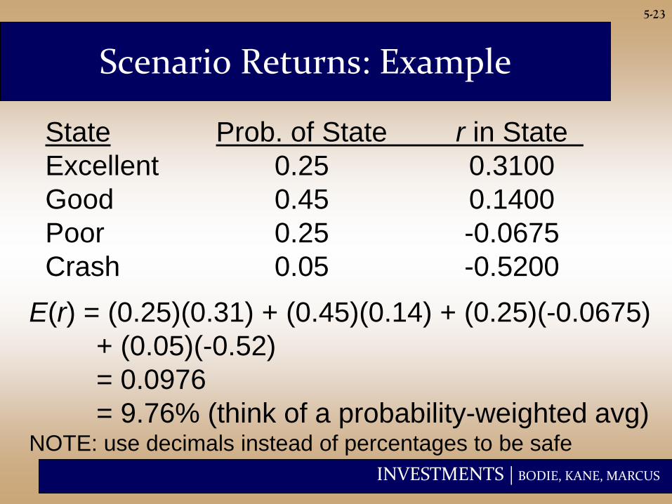
5-23

State Prob. of State r in State

Excellent 0.25 0.3100

Good 0.45 0.1400

Poor 0.25 -0.0675

Crash 0.05 -0.5200

E(r) = (0.25)(0.31) + (0.45)(0.14) + (0.25)(-0.0675)

+ (0.05)(-0.52)

= 0.0976

= 9.76% (think of a probability-weighted avg) NOTE: use decimals instead of percentages to be safe

Scenario Returns: Example


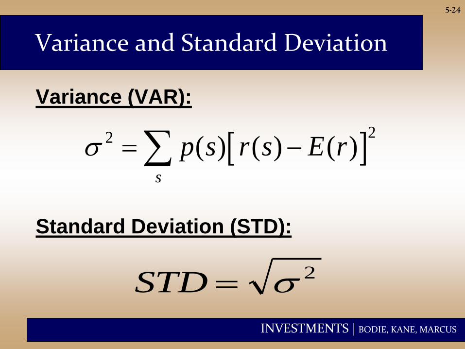
5-24

Variance (VAR):

Variance and Standard Deviation

22 ( ) ( ) ( )

s

p s r s E r

2STD

Standard Deviation (STD):


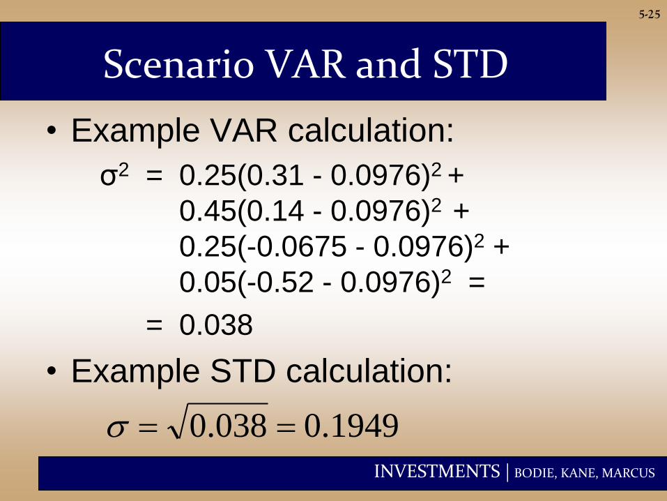
5-25

Scenario VAR and STD

• Example VAR calculation:

σ2 = 0.25(0.31 - 0.0976)2 +

0.45(0.14 - 0.0976)2 +

0.25(-0.0675 - 0.0976)2 +

0.05(-0.52 - 0.0976)2 =

= 0.038

• Example STD calculation:

1949.0038.0


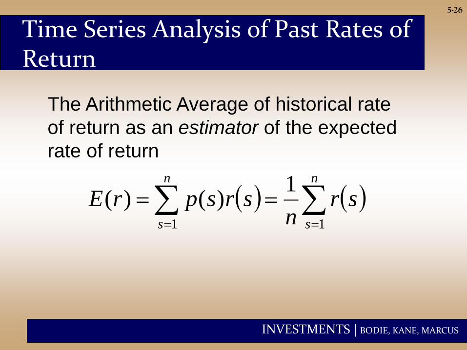
5-26

Time Series Analysis of Past Rates of Return

n

s

n

s

srn

srsprE11

1)()(

The Arithmetic Average of historical rate

of return as an estimator of the expected

rate of return


5-27

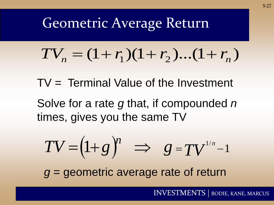
Geometric Average Return

1/1 1 TVggTV nn

TV = Terminal Value of the Investment

g = geometric average rate of return

)1)...(1)(1( 21 nn rrrTV

Solve for a rate g that, if compounded n

times, gives you the same TV


5-28

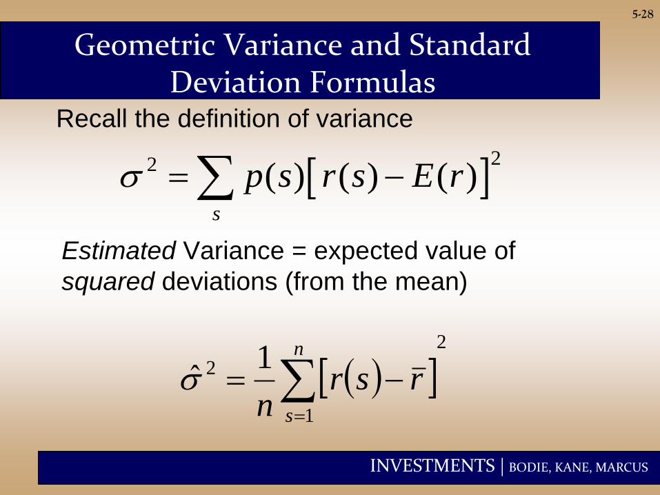
Geometric Variance and Standard Deviation Formulas

Estimated Variance = expected value of

squared deviations (from the mean)

2

1

2 1ˆ

n

s

rsrn

22 ( ) ( ) ( )

s

p s r s E r

Recall the definition of variance


5-29

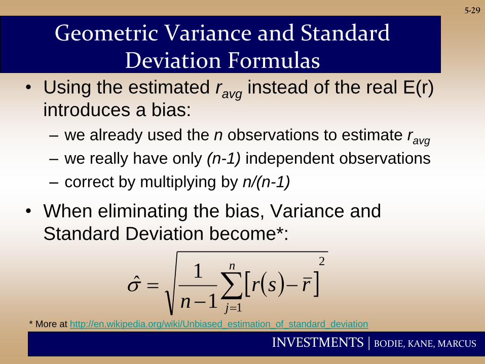
Geometric Variance and Standard Deviation Formulas

• Using the estimated ravg instead of the real E(r)

introduces a bias:

– we already used the n observations to estimate ravg

– we really have only (n-1) independent observations

– correct by multiplying by n/(n-1)

• When eliminating the bias, Variance and

Standard Deviation become*:

2

11

1ˆ

n

j

rsrn

* More at http://en.wikipedia.org/wiki/Unbiased_estimation_of_standard_deviation

http://en.wikipedia.org/wiki/Unbiased_estimation_of_standard_deviation


5-30

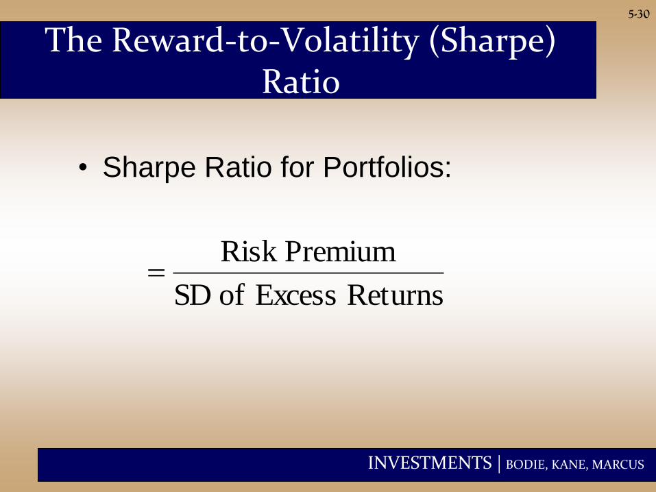
The Reward-to-Volatility (Sharpe) Ratio

• Sharpe Ratio for Portfolios:

Returns Excess of SD

PremiumRisk


5-31

The Normal Distribution

• Investment management math is easier

when returns are normal

– Standard deviation is a good measure of risk

when returns are symmetric

– If security returns are symmetric, portfolio

returns will be, too

– Assuming Normality, future scenarios can be

estimated using just mean and standard

deviation


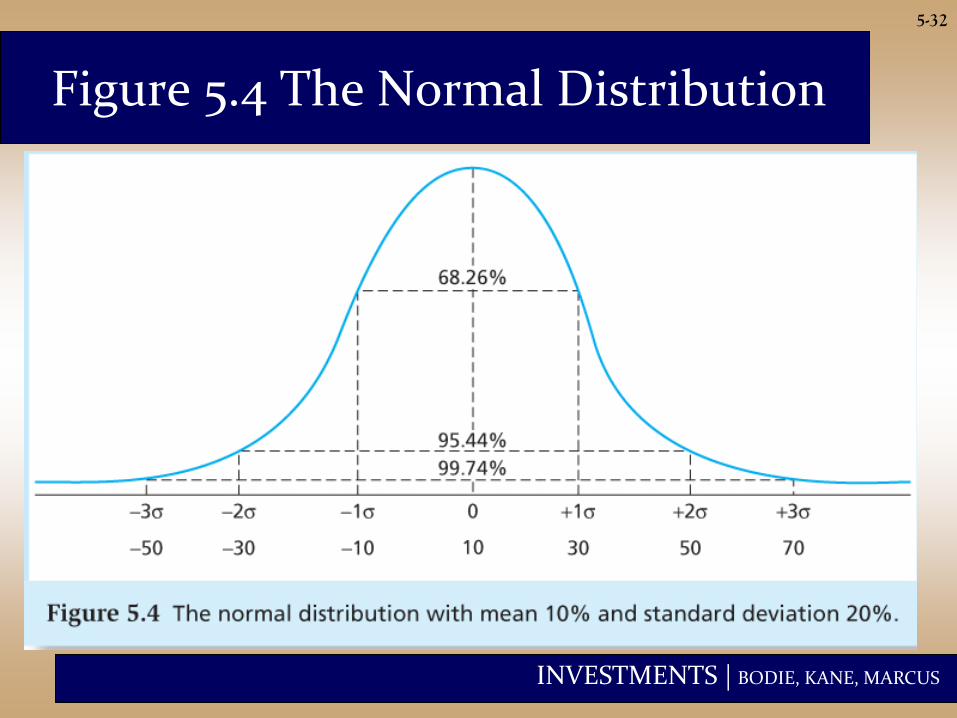
5-32

Figure 5.4 The Normal Distribution


5-33

Normality and Risk Measures

• What if excess returns are not normally

distributed?

– Standard deviation is no longer a complete

measure of risk

– Sharpe ratio is not a complete measure of

portfolio performance

– Need to consider skew and kurtosis


5-34

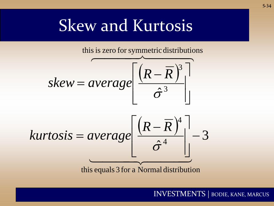
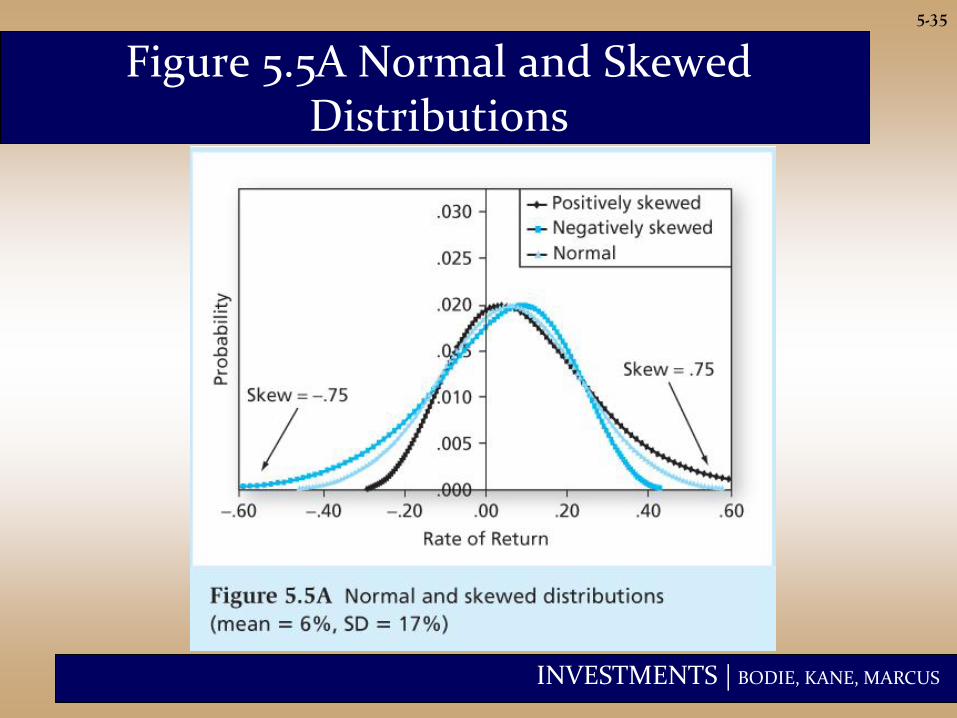
Skew and Kurtosis

3

3

RRaverageskew

3

ˆ 4

4

RRaveragekurtosis

onsdistributi symmetricfor zero is this

ondistributi Normal afor 3 equals this


5-35

Figure 5.5A Normal and Skewed Distributions


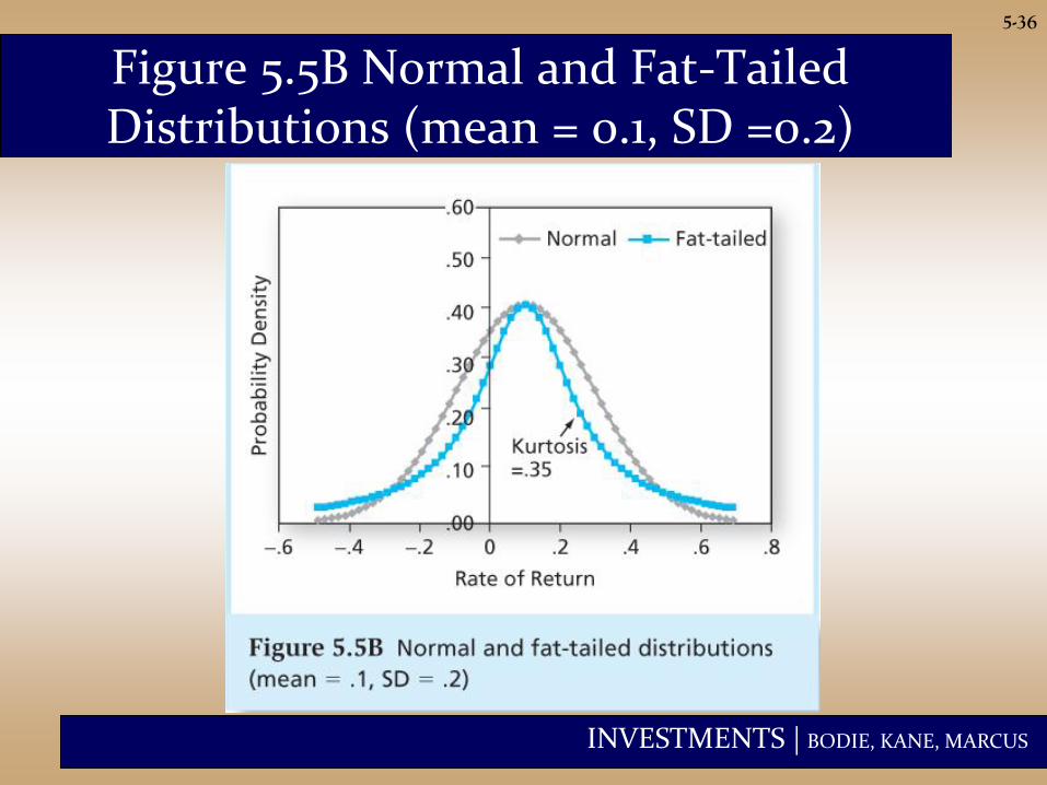
5-36

Figure 5.5B Normal and Fat-Tailed Distributions (mean = 0.1, SD =0.2)


5-37

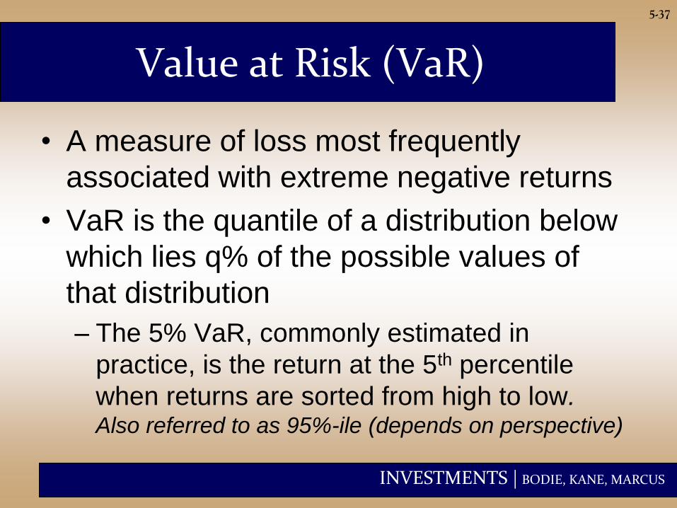
Value at Risk (VaR)

• A measure of loss most frequently

associated with extreme negative returns

• VaR is the quantile of a distribution below

which lies q% of the possible values of

that distribution

– The 5% VaR, commonly estimated in

practice, is the return at the 5th percentile

when returns are sorted from high to low. Also referred to as 95%-ile (depends on perspective)


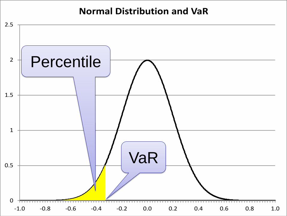
5-38

0

0.5

1

1.5

2

2.5

-1.0 -0.8 -0.6 -0.4 -0.2 0.0 0.2 0.4 0.6 0.8 1.0

Normal Distribution and VaR

Percentile

VaR


5-39

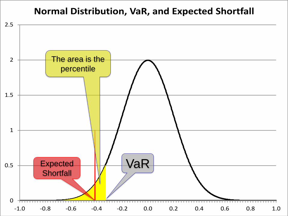
Expected Shortfall (ES)

• a.k.a. Conditional Tail Expectation (CTE)

• More conservative measure of downside

risk than VaR:

– VaR takes the highest return from the worst

cases

– Real life distributions are asymmetric and

have fat tails

– ES takes an average return of the worst cases


5-40

0

0.5

1

1.5

2

2.5

-1.0 -0.8 -0.6 -0.4 -0.2 0.0 0.2 0.4 0.6 0.8 1.0

Normal Distribution, VaR, and Expected Shortfall

Expected

Shortfall

The area is the

percentile

VaR


5-41

Lower Partial Standard Deviation (LPSD) and the Sortino Ratio

• Issues with real life returns:

– Need to look at negative returns separately to

account for asymmetry and fat tails

– Need to consider excess returns: deviations

of returns from the risk-free rate.

• LPSD: similar to usual standard deviation,

but uses only negative deviations from rf

• Sortino Ratio replaces Sharpe Ratio


A game with a coin

Let’s play a game: flip a (non-fair) coin, and

receive $1 if heads

• Assume Pr[Heads]= p (for example p=50%)

Q. What is the game’s expected outcome?

Q. What is the Variance?

Q. What is the St.Dev?

5-42


A game with two coins

Let’s play a game: flip 2 fair coins, and

receive $1 for each head

Q. What is the portfolio expected return?

Q. What is the portfolio Variance?

Q. What is the portfolio St.Dev?

5-43


A lot more coins

Let’s play a game: flip 30 fair coins, and

receive $1 for each head.



Q. What is the portfolio St.Dev?

5-44


A Portfolio of 2 stocks

• Portfolio = 0.5 * A + 0.5 * B

• A: rA = 0.08 StDevA = 0.1

• B: rB = 0.10 StDevB = 0.1



Q. What is the portfolio Standard Deviation?

5-45


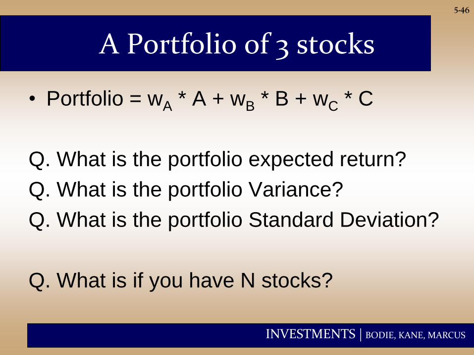
A Portfolio of 3 stocks

• Portfolio = wA * A + wB * B + wC * C



Q. What is the portfolio Standard Deviation?

Q. What is if you have N stocks?

5-46


S

5-47

(A)

(B) (C)

(D) (E)

30% (A) 50% (B) 20% (D)

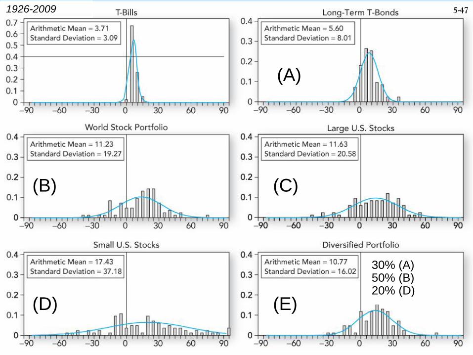
1926-2009


5-48

Historic Returns on Risky Portfolios

• Returns appear approximately normally distributed

• Returns are lower over the most recent half of the period (1986-2009)

• SD for small stocks became smaller; SD for long-term bonds got bigger

• Better diversified portfolios have higher Sharpe Ratios

• Negative skew


5-49

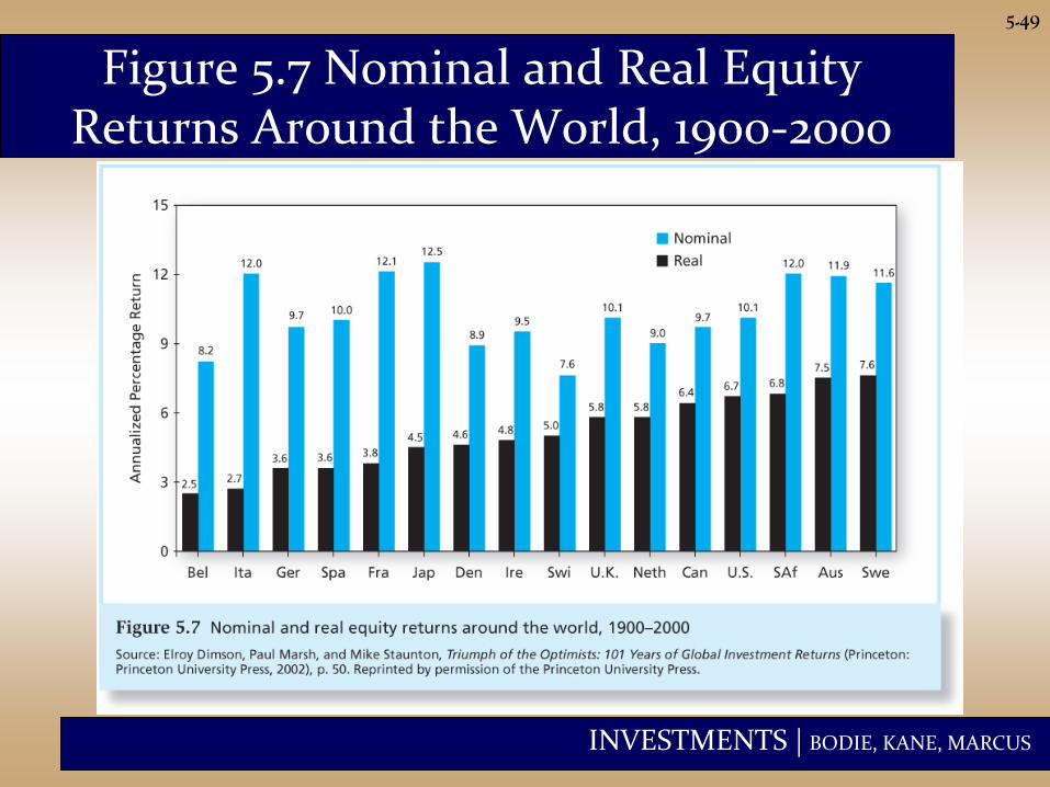
Figure 5.7 Nominal and Real Equity Returns Around the World, 1900-2000


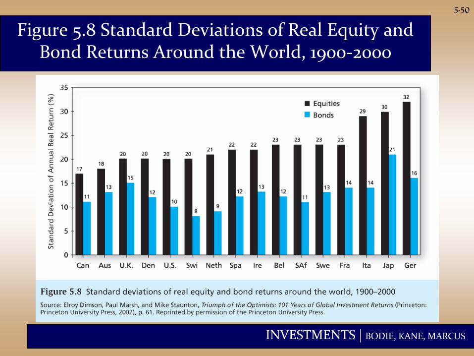
5-50

Figure 5.8 Standard Deviations of Real Equity and Bond Returns Around the World, 1900-2000


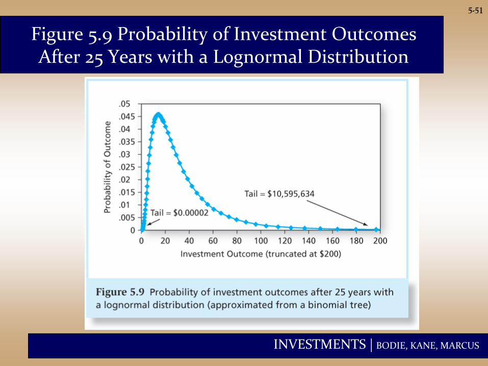
5-51

Figure 5.9 Probability of Investment Outcomes After 25 Years with a Lognormal Distribution


5-52

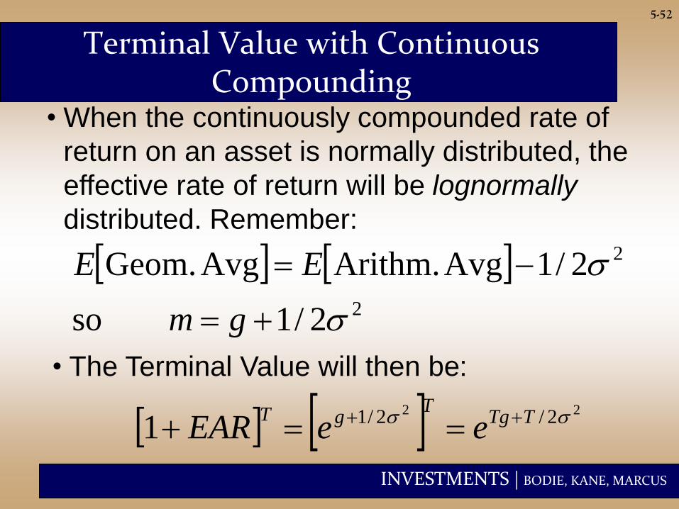
Terminal Value with Continuous Compounding

• When the continuously compounded rate of

return on an asset is normally distributed, the

effective rate of return will be lognormally

distributed. Remember:

22 2/2/11 TTgT

gTeeEAR

2

2

2/1 so

2/1Avg Arithm.Avg Geom.

gm

EE

• The Terminal Value will then be:


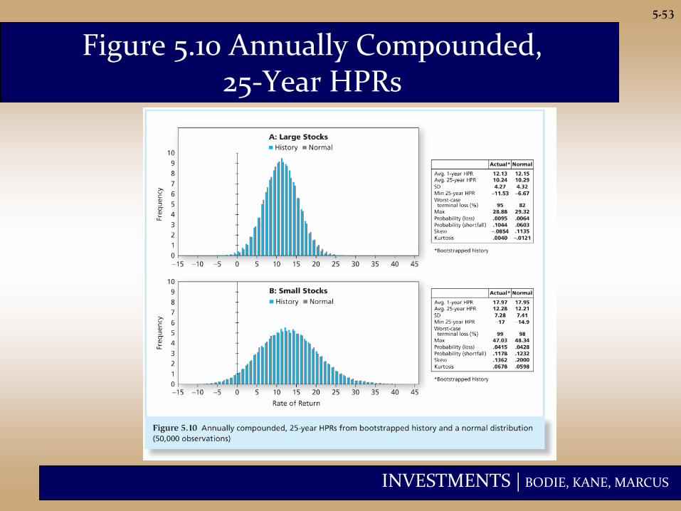
5-53

Figure 5.10 Annually Compounded, 25-Year HPRs


5-54

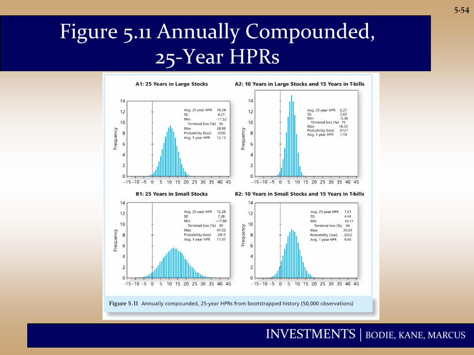
Figure 5.11 Annually Compounded, 25-Year HPRs


5-55

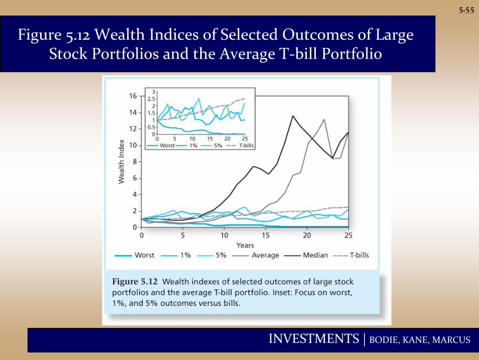
Figure 5.12 Wealth Indices of Selected Outcomes of Large Stock Portfolios and the Average T-bill Portfolio

Documents

CHAPTER 5leeds-faculty.colorado.edu/.../FNCE4030-Fall-2012-ch05-handouts.pdfINVESTMENTS | BODIE, KANE, MARCUS 5-2 Interest Rate Determinants • Supply –Households • Demand –Businesses