Embed Size (px)
DESCRIPTION
CHAPTER 6. The Three Common Approaches for Calculating Value at Risk. INTRODUCTION. VaR is is a good measure of risk it combines information on the sensitivity of the value to changes in market-risk factors with information on the probable amount of change in those factors. - PowerPoint PPT Presentation
Citation preview

CHAPTER 6
The Three Common Approaches for Calculating Value at Risk

INTRODUCTION
• VaR is is a good measure of risk– it combines information on the sensitivity of the value to changes
in market-risk factors with information on the probable amount of change in those factors.
– VaR tries to answer the question: how much could we lose today given our current position and the possible changes in the market?
– VaR formalizes that question into the calculation of the level of loss that is so bad that there is only a 1 in 100 chance of there being a loss worse than the calculated VaR.
– VaR estimates this level by knowing the current value of the portfolio and calculating the probability distribution of changes in the value over the next trading day.
– From the probability distribution we can read the confidence level for the 99-percentile loss.
INTRODUCTION
• To estimate the value's probability distribution, we use two sets of information. the current position, or holdings, in the bank's trading portfolio, and an estimate of the probability distribution of the price changes over the next day.
• The estimate of the probability distribution of the price changes is based on the distribution of price changes over the last few weeks or months.
• The goal of this chapter is to explain how to calculate VaR using the three methods that are in common use:– Parametric VaR– Historical Simulation– Monte CarloSimulation.
LIMITATIONS SHARED BY ALL THREEMETHODS
• It is important to note that while the three calculation methods differ, they do share common attributes and limitations.
• Each approach uses market-risk factors– Risk factors are fundamental market rates that can be derived
from the prices of securities being traded– Typically, the main risk factors used are interest rates, foreign
exchange rates, equity indices, commodity prices, forward prices, and implied volatilities
– By observing this small number of risk factors, we are able to calculate the price of all the thousands of different securities held by the bank
– This risk-factor approach uses less data than would be required if we tried to collect historical price information for every security.
LIMITATIONS SHARED BY ALL THREEMETHODS
• Each approach uses the distribution of historical price changes to estimate the probability distributions. – This requires a choice of historical horizon for
the market data– how far back should we go in using historical
data to calculate standard deviations?– This is a trade-off between having large
amounts of information or fresh information
LIMITATIONS SHARED BY ALL THREEMETHODS
• Because VaR attempts to predict the future probability distribution, it should use the latest market data with the latest market structure and sentiment– However, with a limited amount of data, the es
timates become less accurate– There is less chance of having data that conta
ins those extreme, rare market movements which are the ones that cause the greatest losses

LIMITATIONS SHARED BY ALL THREEMETHODS
• Each approach has the disadvantage of assuming that past relationships between the risk factors will be repeated– it assumes that factors that have tended to
move together in the past will move together in the future
LIMITATIONS SHARED BY ALL THREEMETHODS
• Each approach has strengths and weaknesses when compared to the others, as summarized in Figure 6-1– The degree to which the circles are shaded
corresponds to the strength of the approach– The factors evaluated in the table are
• the speed of computation• the ability to capture nonlinearity
– Nonlinearity refers, to the price change not being at linear function of the change in the risk factors. This is especially important for options
• the ability to capture non-Normality– non-Normality refers to the ability to calculate the potential
changes in risk factors without assuming that they have a Normal distribution
• the independence from historical data

LIMITATIONS SHARED BY ALL THREEMETHODS

PARAMETRIC VAR
• Parametric VaR is also known as Linear VaR, Variance-Covariance VaR
• The approach is parametric in that it assumes that the probability distribution is Normal and then requires calculation of the variance and covariance parameters.
• The approach is linear in that changes in instrument values are assumed to be linear with respect to changes in risk factors.
• For example, for bonds the sensitivity is described by duration, and for options it is described by the Greeks
PARAMETRIC VAR
• The overall Parametric VaR approach is as follows:– Define the set of risk factors that will be sufficient to calculate the
value of the bank's portfolio– Find the sensitivity of each instrument in the portfolio to each risk
factor– Get historical data on the risk factors to calculate the standard d
eviation of the changes and the correlations between them– Estimate the standard deviation of the value of the portfolio by m
ultiplying the sensitivities by the standard deviations, taking into account all correlations
– Finally, assume that the loss distribution is Normally distributed, and therefore approximate the 99% VaR as 2.32 times the standard deviation of the value of the portfolio
PARAMETRIC VAR
• Parametric VaR has two advantages:– It is typically 100 to 1000 times faster to calcul
ate Parametric VaR compared with Monte Carlo or Historical Simulation.
– Parametric VaR allows the calculation of VaR contribution, as explained in the next chapter.
PARAMETRIC VAR
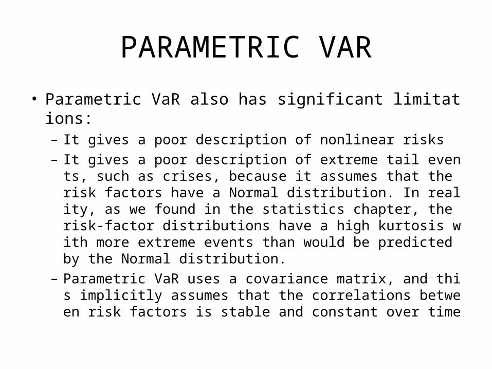
• Parametric VaR also has significant limitations:– It gives a poor description of nonlinear risks– It gives a poor description of extreme tail events, such
as crises, because it assumes that the risk factors have a Normal distribution. In reality, as we found in the statistics chapter, the risk-factor distributions have a high kurtosis with more extreme events than would be predicted by the Normal distribution.
– Parametric VaR uses a covariance matrix, and this implicitly assumes that the correlations between risk factors is stable and constant over time

PARAMETRIC VAR
• To give an intuitive understanding of Parametric VaR, we have provided three worked-out examples.
• The examples are fundamentally quite simple, but they intro-duce the method of calculating Parametric VaR.
• There are a lot of equations, but the underlying math is mostly algebra rather than complex statistics or calculus
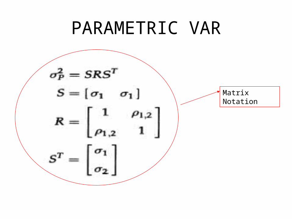
• Three different notations are used in this chapter– Algebraic– Summation– matrix.
PARAMETRIC VAR
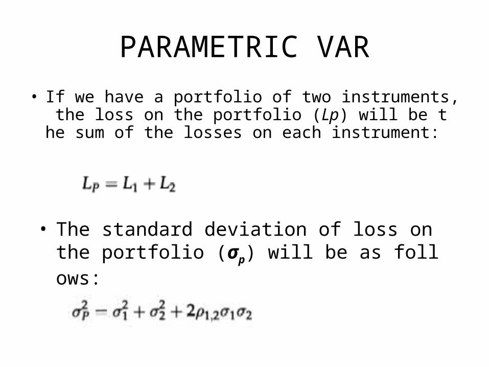
• If we have a portfolio of two instruments, the loss on the portfolio (Lp) will be the sum of the losses on each instrument:
• The standard deviation of loss on the portfolio (σp) will be as follows:

PARAMETRIC VARAlgebraic Notation
Summation Notation
PARAMETRIC VAR
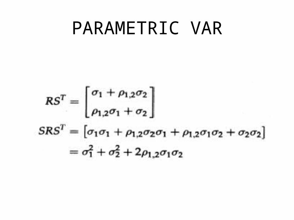
Matrix Notation
PARAMETRIC VAR
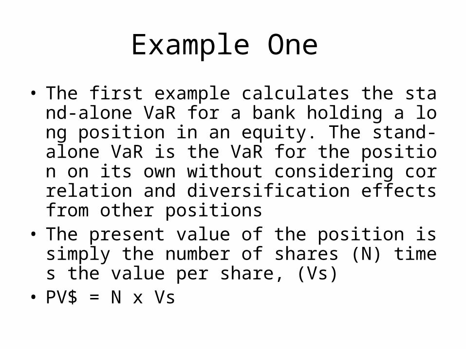
Example One
• The first example calculates the stand-alone VaR for a bank holding a long position in an equity. The stand-alone VaR is the VaR for the position on its own without considering correlation and diversification effects from other positions
• The present value of the position is simply the number of shares (N) times the value per share, (Vs)
• PV$ = N x Vs

Example One• The change in the value of the position is simply the number of shar
es multiplied by the change in the value of each share:
• ΔPV$ = N x ΔVs• • The standard deviation of the value is the number of shares multipli
ed by the standard deviation of the value of each share
• σv = N x σs
• we have assumed that the value changes are Normally distributed, there will be a 1chance that the loss is more than 2.32 standard deviations; therefore, we can calculatethe 99 VaR as follows
• VaR = 2.32 x N xσs

Example Two
• As a slightly more complex example, consider a government bond held by a U.K. bank denominated in British pounds with a single payment.
• The present value in pounds (PVp) is simply the value of the cash flow in pounds (Cp) at time t discounted according to sterling interest rates for that maturity, rp:

Example Twopresent value
The derivative of PVp with respect to rp
Example Two
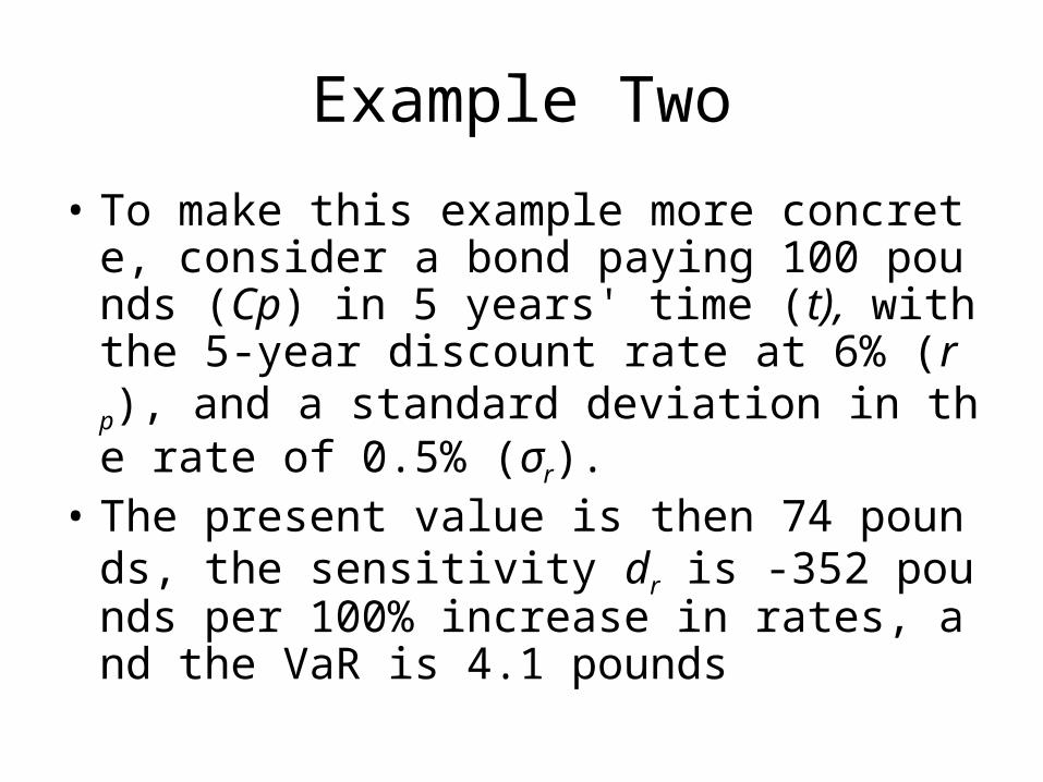
• To make this example more concrete, consider a bond paying 100 pounds (Cp) in 5 years' time (t), with the 5-year discount rate at 6% (rp), and a standard deviation in the rate of 0.5% (σr).
• The present value is then 74 pounds, the sensitivity dr is -352 pounds per 100% increase in rates, and the VaR is 4.1 pounds

Example Two

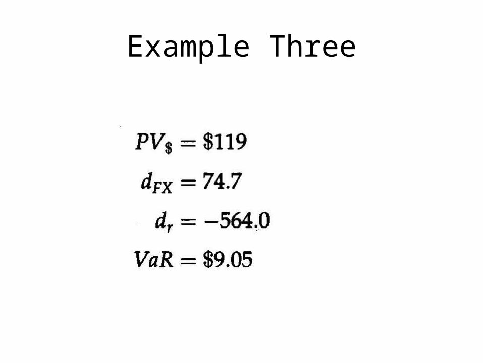
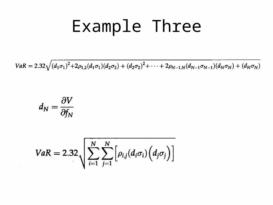
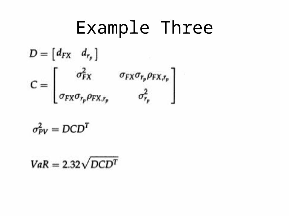
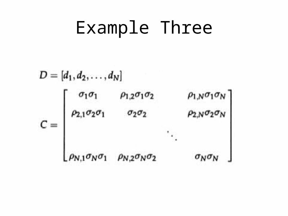
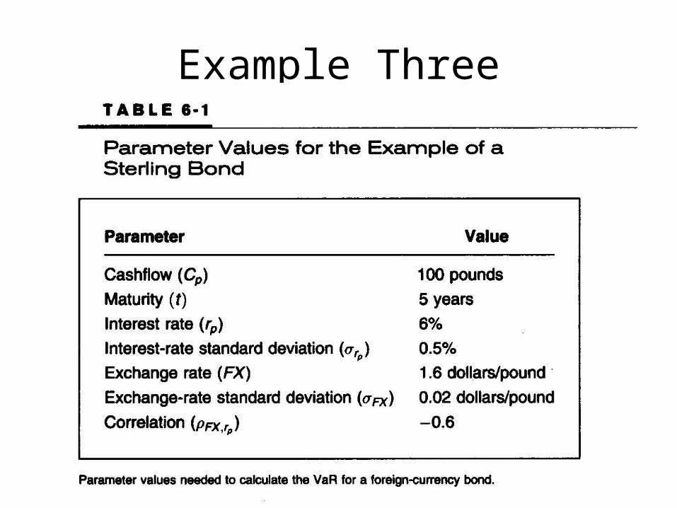
Example Three
• The two examples above were simple because they had only one risk factor
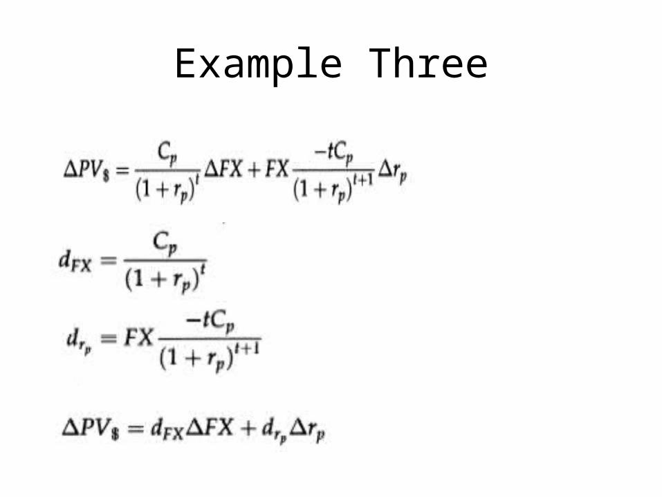
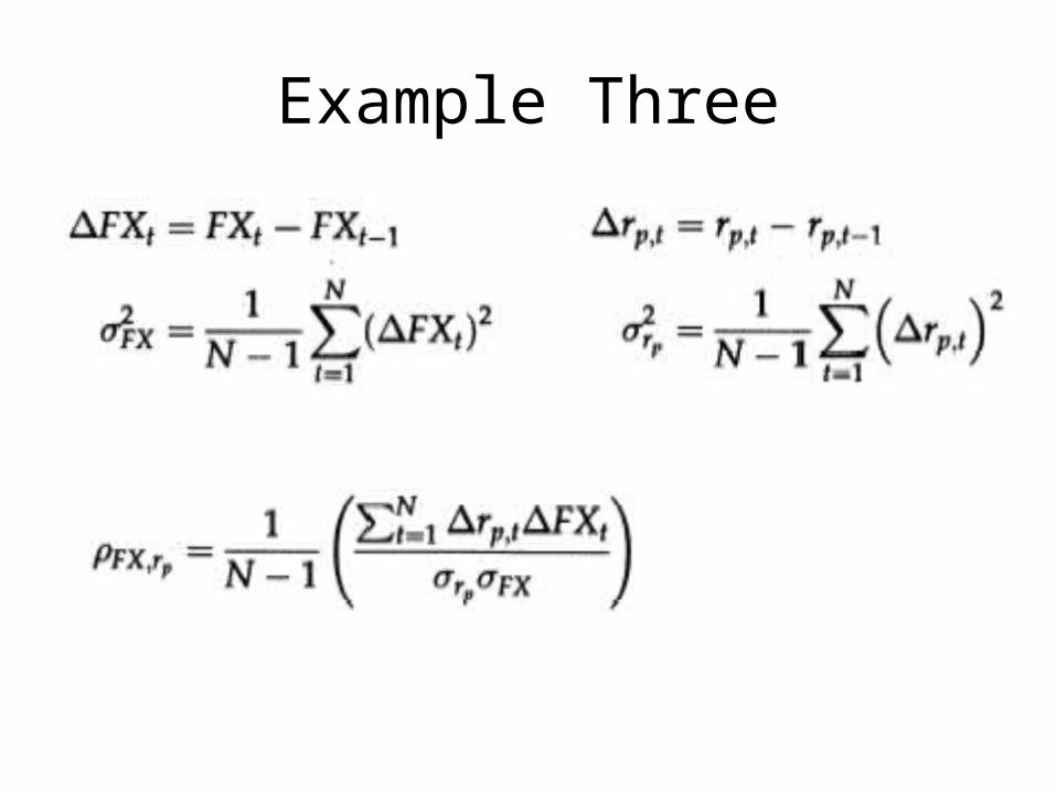
• Now let us consider a multidimensional case: the same simple bond as before, but now held by a U.S. bank.
• The U.S. bank is exposed to two risks: changes due to sterling interest rates and changes due to the pound-dollar exchange rate.
• The value of the bond in dollars is the value in pounds multiplied by the FX rate

Example Three
Example Three

Example Three
Example Three


Example Three

Example Three
Example Three
Example Three
Example Three

Example Three
Example Three
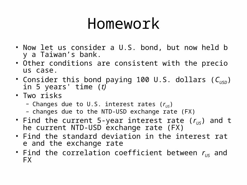
Homework
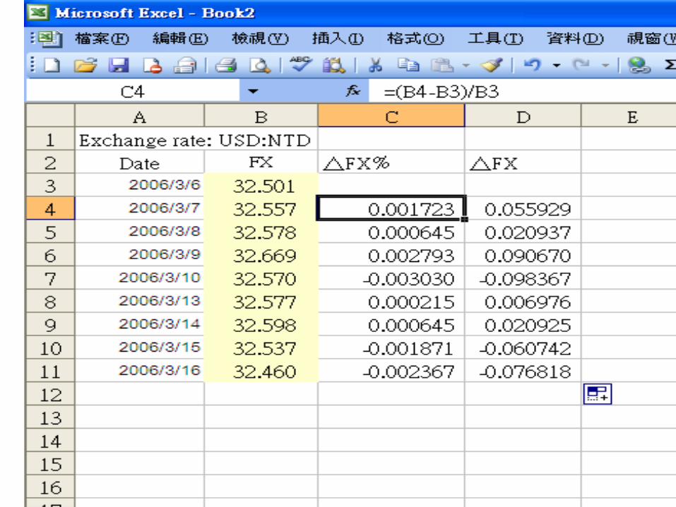
• Now let us consider a U.S. bond, but now held by a Taiwan’s bank.
• Other conditions are consistent with the precious case. • Consider this bond paying 100 U.S. dollars (CUSD) in 5 ye
ars' time (t)• Two risks
– Changes due to U.S. interest rates (rUS) – changes due to the NTD-USD exchange rate (FX)
• Find the current 5-year interest rate (rUS) and the current NTD-USD exchange rate (FX)
• Find the standard deviation in the interest rate and the exchange rate
• Find the correlation coefficient between rUS and FX

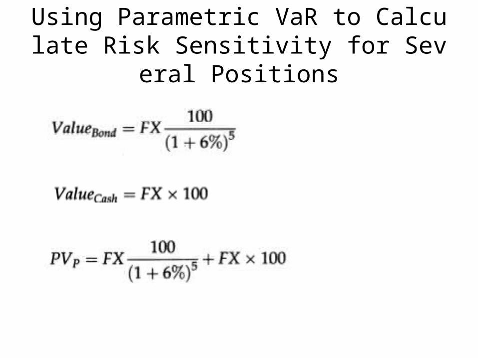
Using Parametric VaR to Calculate Risk Sensitivity for Several Positions
• In the example above, we had one security that was sensitive to two different risk factors.
• If the portfolio is made up of several securities, each of which is affected by the same risk factor, then the sensitivity of the portfolio to the risk factor is simply the sum of these sensitivities for the individual positions.
• For example, consider a portfolio holding our example 100-pound five-year bond and 100 pounds of cash
Using Parametric VaR to Calculate Risk Sensitivity for Several Positions

Using Parametric VaR to Calculate Risk Sensitivity for Several Positions

Using Parametric VaR to Calculate Risk Sensitivity for Several Positions
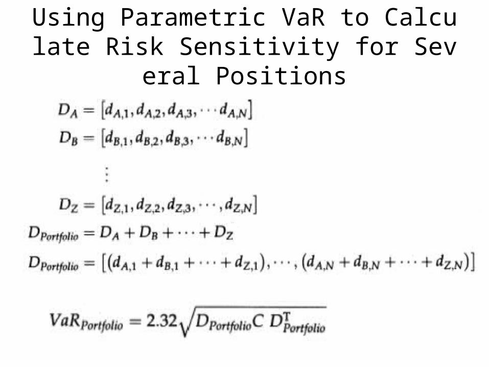
Using Parametric VaR to Calculate Risk Sensitivity for Several Positions

Homework
• Now let us consider a bond portfolio with a U.S. bond and a U.K. bond,
• The bond portfolio is held by a Taiwan’s bank.• Other conditions are consistent with the precious case. • Consider the US and UK bonds paying 100 US dollars
(CUSD) and 100 British pound (CBP), respectively, in 5 years' time (t)
• Four risk factors– Changes due to U.S. interest rates (rUS) – changes due to the NTD-USD exchange rate (FXUSD)– Changes due to U.K. interest rates (rUK) – changes due to the NTD-BP exchange rate (FXBP)
HISTORICAL-SIMULATION VAR
• Conceptually, historical simulation is the most simple VaR technique, but it takes significantly more time to run than parametric VaR.
• The historical-simulation approach takes the market data for the last 250 days and calculates the percent change for each risk factor on each day
• Each percentage change is then multiplied by today's market values to present 250 scenarios for tomorrow's values.
• For each of these scenarios, the portfolio is valued using full, nonlinear pricing models. The third-worst day is the selected as being the 99% VaR.
HISTORICAL-SIMULATION VAR
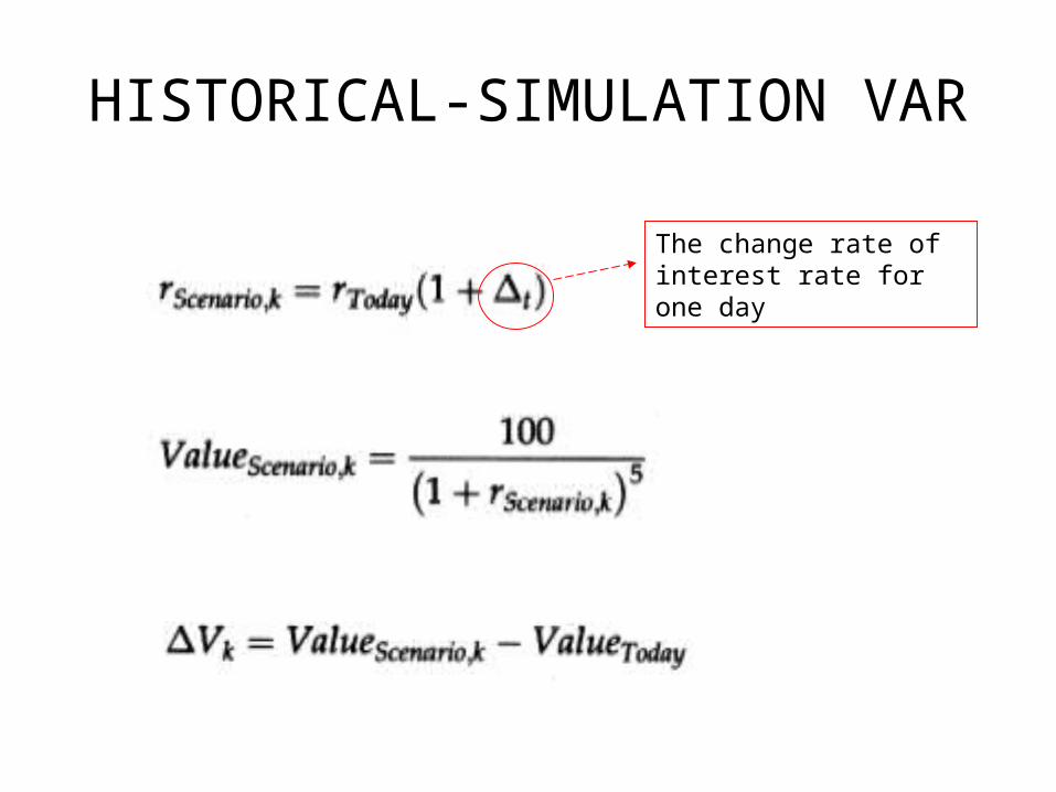
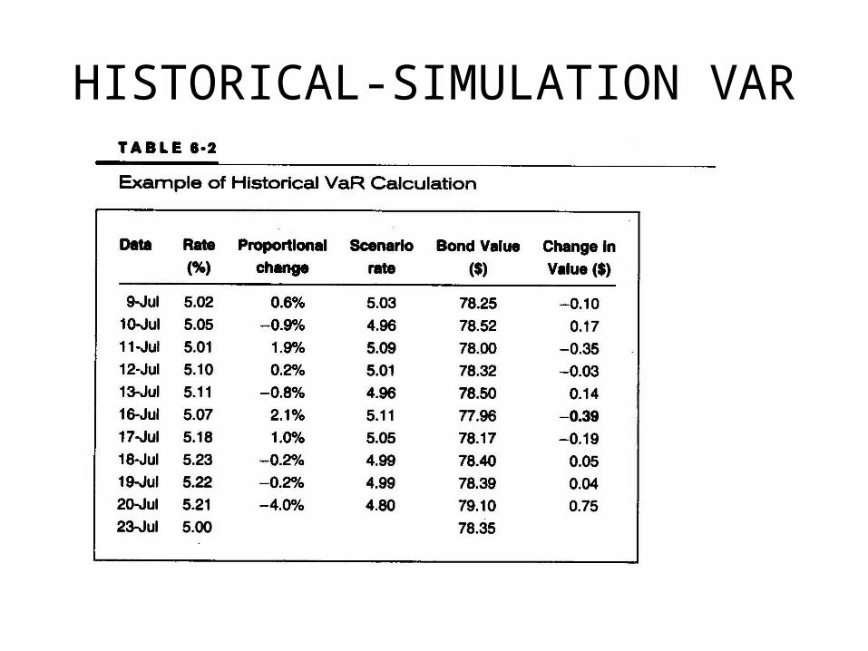
• As an example, let's consider calculating the VaR for a five-year, zero-coupon bond paying $100
• We start by looking back at the previous trading days and noting the five year rate on each day.
• We then calculate the proportion by which the rate changed from one day to the next
HISTORICAL-SIMULATION VAR
The change rate of interest rate for one day
HISTORICAL-SIMULATION VAR
Homework
• Consider a Taiwan bond held by a Taiwan’s bank.
• Other conditions are consistent with the precious case.
• Consider this bond paying 100 NT dollars (CNTD) in 5 years' time (t)
• One risk factor– Changes due to Taiwan interest rates (rTAIWAN)
• Use the historical simulation approach to calculate the VaR
• Use one-year historical data at least
HISTORICAL-SIMULATION VAR
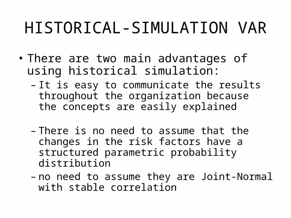
• There are two main advantages of using historical simulation:– It is easy to communicate the results
throughout the organization because the concepts are easily explained
– There is no need to assume that the changes in the risk factors have a structured parametric probability distribution
– no need to assume they are Joint-Normal with stable correlation
HISTORICAL-SIMULATION VAR
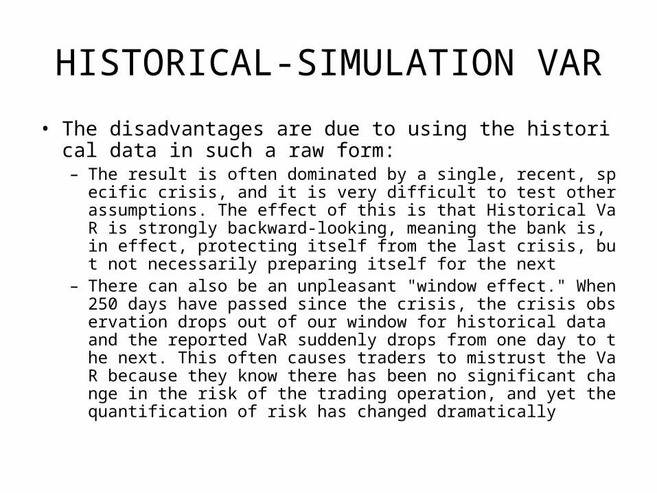
• The disadvantages are due to using the historical data in such a raw form:– The result is often dominated by a single, recent, specific crisis,
and it is very difficult to test other assumptions. The effect of this is that Historical VaR is strongly backward-looking, meaning the bank is, in effect, protecting itself from the last crisis, but not necessarily preparing itself for the next
– There can also be an unpleasant "window effect." When 250 days have passed since the crisis, the crisis observation drops out of our window for historical data and the reported VaR suddenly drops from one day to the next. This often causes traders to mistrust the VaR because they know there has been no significant change in the risk of the trading operation, and yet the quantification of risk has changed dramatically
MONTE CARLO SIMULATION VAR
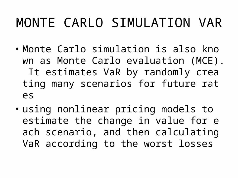
• Monte Carlo simulation is also known as Monte Carlo evaluation (MCE). It estimates VaR by randomly creating many scenarios for future rates
• using nonlinear pricing models to estimate the change in value for each scenario, and then calculating VaR according to the worst losses

MONTE CARLO SIMULATION VAR
• Monte Carlo simulation has two significant advantages:– Unlike Parametric VaR, it uses full pricing mo
dels and can therefore capture the effects of nonlinearities
– Unlike Historical VaR, it can generate an infinite number of scenarios and therefore test many possible future outcomes

MONTE CARLO SIMULATION VAR
• Monte Carlo has two important disadvantages:– The calculation of Monte Carlo VaR can take
1000 times longer than Parametric VaR because the potential price of the portfolio has to be calculated thousands of times
– Unlike Historical VaR, it typically requires the assumption that the risk factors have a Normal or Log-Normal distribution.
MONTE CARLO SIMULATION VAR
• The Monte Carlo approach assumes that there is a known probability distribution for the risk factors.
• The usual implementation of Monte Carlo assumes a stable, Joint-Normal distribution for the risk factors.
• This is the same assumption used for Parametric VaR.
• The analysis calculates the covariance matrix for the risk factors in the same way as Parametric VaR

MONTE CARLO SIMULATION VAR
• But unlike Parametric VaR– Decomposes the covariance matrix and ensures that t
he risk factors are correlated in each scenario– The scenarios start from today's market condition and
go one day forward to give possible values at the end of the day
– Full, nonlinear pricing models are then used to value the portfolio under each of the end-of-day scenarios.
– For bonds, nonlinear pricing means using the bond-pricing formula rather than duration
– for options, it means using a pricing formula such as Black-Scholes rather than just using the Greeks.
MONTE CARLO SIMULATION VAR
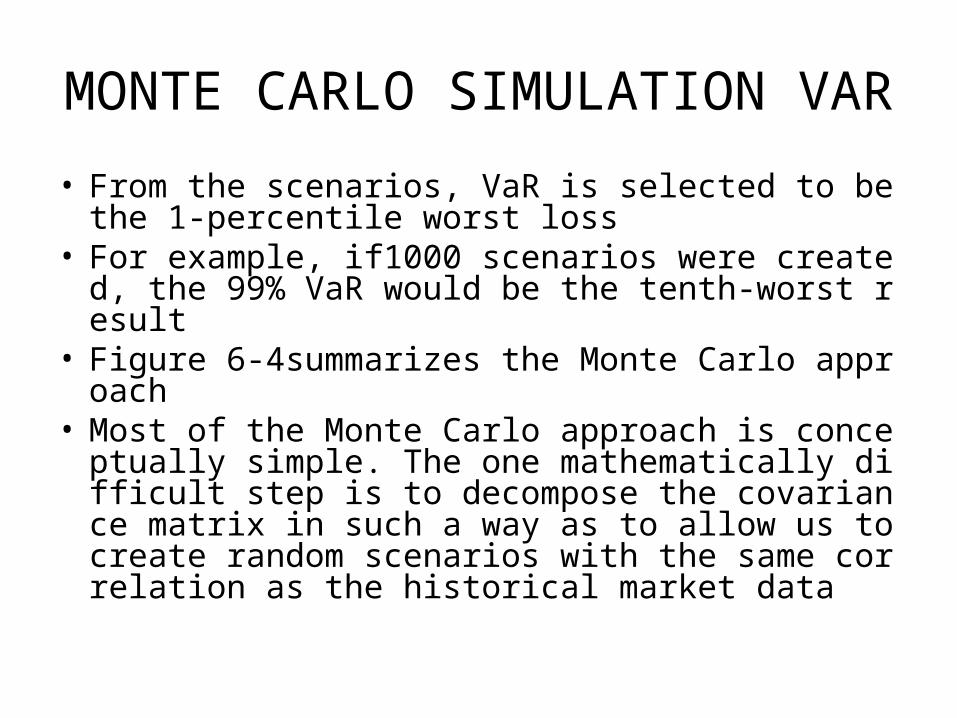
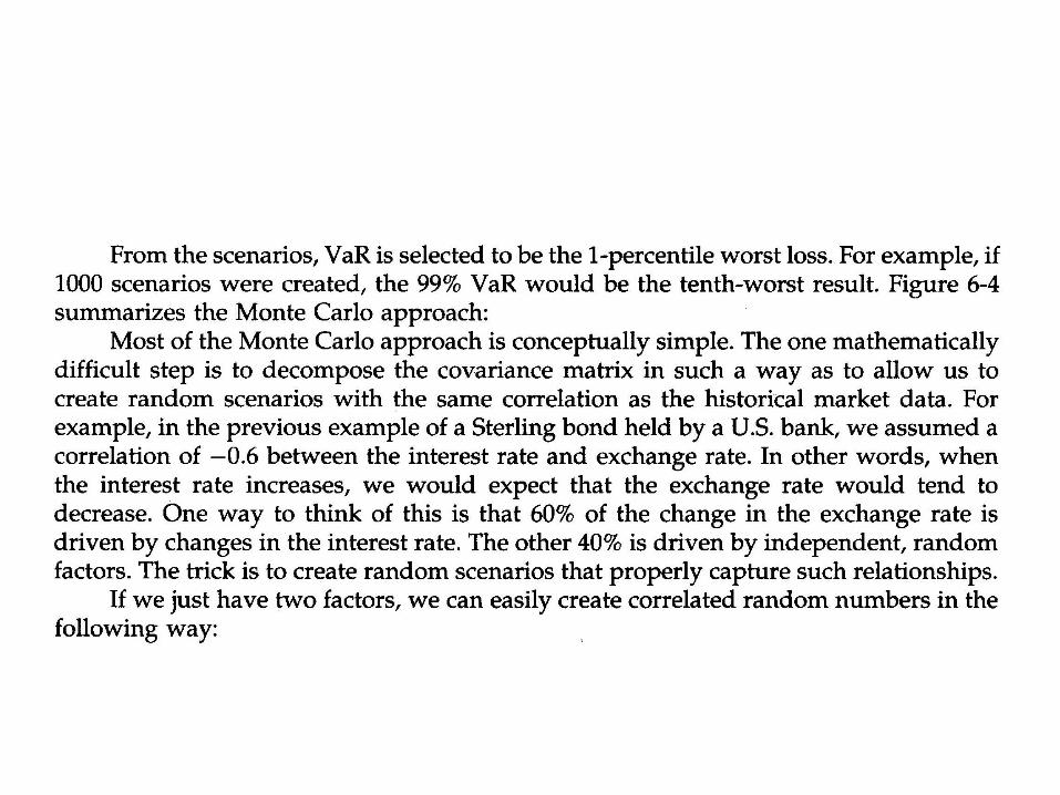
• From the scenarios, VaR is selected to be the 1-percentile worst loss
• For example, if1000 scenarios were created, the 99% VaR would be the tenth-worst result
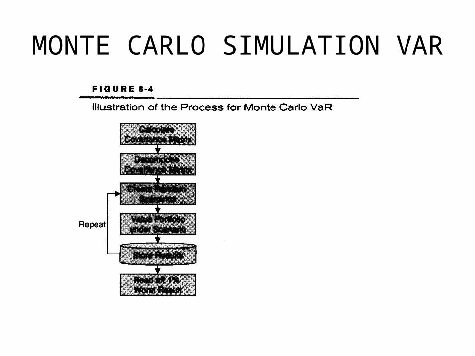
• Figure 6-4summarizes the Monte Carlo approach
• Most of the Monte Carlo approach is conceptually simple. The one mathematically difficult step is to decompose the covariance matrix in such a way as to allow us to create random scenarios with the same correlation as the historical market data
MONTE CARLO SIMULATION VAR

MONTE CARLO SIMULATION VAR
• For example, in the previous example of a Sterling bond held by a U.S. bank, we assumed a correlation of -0.6 between the interest rate and exchange rate
• In other words, when the interest rate increases, we would expect that the exchange rate would tend to decrease.
• One way to think of this is that 60% of the change in the exchange rate is driven by changes in the interest rate. The other 40% is driven by independent, random factors.
• The trick is to create random scenarios that properly capture such relationships
MONTE CARLO SIMULATION VAR
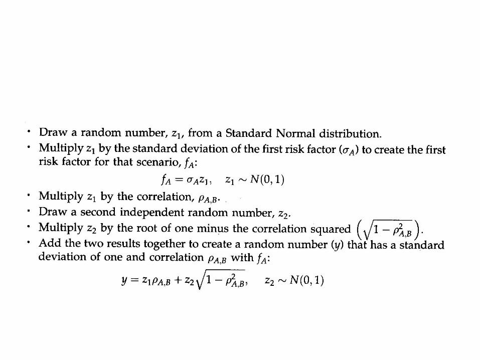
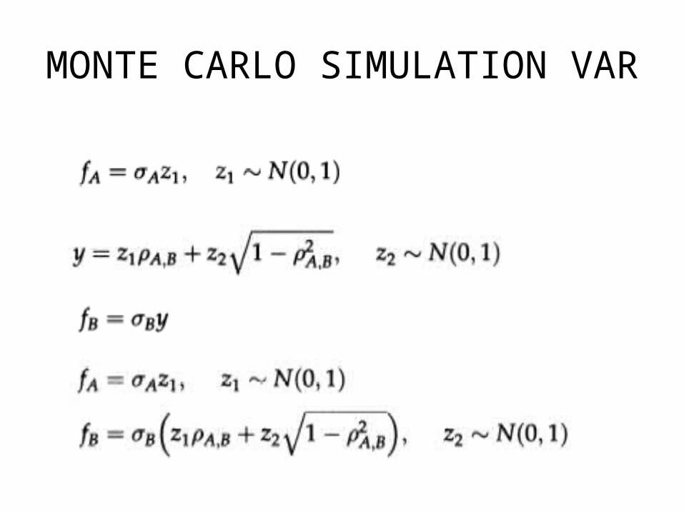
• If we just have two factors, we can easily create correlated random numbers in a simple way:
• Please refer to P120


MONTE CARLO SIMULATION VAR
Example Three

Example Three
MONTE CARLO SIMULATION VAR
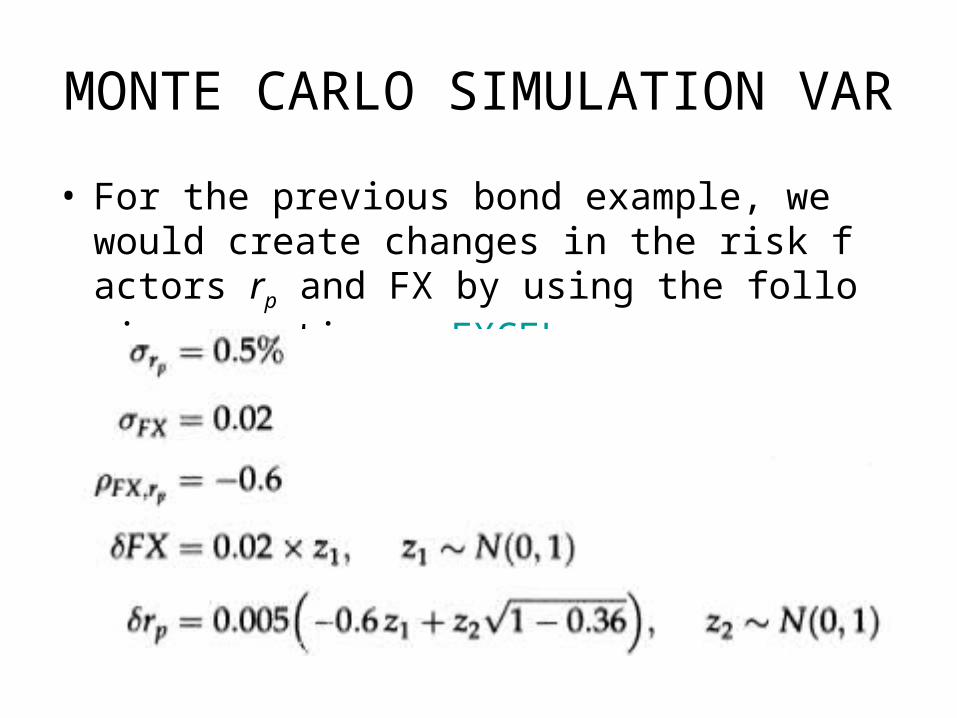
• For the previous bond example, we would create changes in the risk factors rp and FX by using the following equations: EXCEL

Homework
• Find the realized data to redo the sample example in the previous homework
• Three approaches are asked to apply– Parametric VaR– Historical VaR– Monte Carlo VaR
• Compare the differences among them

Homework
• Now let us consider a U.S. bond, but now held by a Taiwan’s bank.
• Other conditions are consistent with the precious case.
• Consider this bond paying 100 U.S. dollars (CUS
D) in 5 years' time (t)
• Two risk factors– Changes due to U.S. interest rates (rUS)
– changes due to the NTD-USD exchange rate (FX)

Quick Quiz
• Four popular limitations for VaR ?– Calculation speed– Non-normality– Nonlinearity– Too heavily dependent on historical data
• Three common approaches for VaR– The main advantage/disadvantage for each of
them?

LIMITATIONS SHARED BY ALL THREEMETHODS