197

Chapter 6

BUILDING ON THE COUNTERCYCLICAL BUFFERCONSENSUS: AN EMPIRICAL TEST FOR THE PHILIPPINES

ByRoselle R. Manalo1

1. Introduction

The global financial crisis that began in 2007 highlighted the weaknesses inthe prevailing regulatory framework for banks. In particular, the crisis emphasisedthe need to address the procyclical nature of banks’ behaviour, with the financialsystem amplifying the business cycle by boosting credit in good times andcontracting credit in bad times. Prior to a crisis, risks are deemed low and creditexpanded rapidly which usually requires low amount of capital. During a crisis,the measure of banks’ riskiness climbs, prompting for higher capitalisation thatis more costly and difficult to source during stress period. Against suchenvironment, existing regulations on bank capitalization have somehow increasedthe pressure for banks to reduce the size of their balance sheets through sharpdeleveraging and constriction of credit supply, which negatively affects overalleconomic activity.2

The recent crisis also showed that static capital requirements are notenough.3 Loan loss provisions and capital ratio requirements, which fail to increasein economic booms, contribute to the procyclicality of the financial system. Borio,et al. (2010) noted that financial stability will be enhanced if such provisioningwill also increase in good times, tracking risks better and acting as a built-in

________________1. Roselle R. Manalo is Bank Officer V of the Department of Economic Research (DER) of

the Bangko Sentral ng Pilipinas (BSP). The views expressed in this paper are those of theauthor and do not necessarily represent those of the BSP or BSP policy. The author ismost thankful for the technical assistance provided by Mauro E. Jasmin, Jay G. Pineda,and Merzinaida Donovan and helpful comments of Evelyn R. Santos.

2. Chen, D. X. and I. Christensen, (2010), “The Countercyclical Bank Capital Buffer: Insightsfor Canada,” Bank of Canada Financial System Review.

3. Riksbank Studies, “Countercyclical Capital Buffers as a Macroprudential Instrument,”December 2012, p. 7.

198

stabiliser when capital is generally cheaper and easier to raise in normal timesthan in recessions.4

In reducing the procyclicality of bank lending to improve bank’s capacity towithstand future losses and help maintain the continued flow of credit in theeconomy, the Basel Committee on Banking Supervision (BCBS) in 2010 finalisedthe third installment of the Basel Accords which include among others theestablishment of a countercyclical capital buffer (CCCB).5

In the Philippines, where the banking sector remains the core of the financialsystem and the primary source of credit for the economy (see Annex Table 1),the establishment of a CCCB appears beneficial. Banks in the country providealmost 80% of credit with the total loan portfolio amounting to P4,892 billion asof end-December 2013. Domestic banks capture the largest share of the physicallandscape at 98% while the rest of the 2% are foreign banks. In 2013, bankfunds are channeled to real estate, renting and business activities (RERBA) andfinancial intermediation sectors.6 The said sectors accounted for the highestshares in the total loan portfolio (TLP) of the banking system at 18.5% and17.0%, respectively, followed by loans to the manufacturing at 13.7% andwholesale and retail trade at 12.8%. Loans extended to agriculture, on the otherhand, comprised 4.4% of the banking system’s TLP.7

With banks as the primary provider of funds in the Philippines, any failureto efficiently intermediate in the system can have significant adverse effect tothe economy. This is evidenced by the substantial losses incurred by the publicsector in periods where the government has to provide liquidity and guaranteesto bring stability to the system. For instance, Gochoco-Bautista (2000) notedthat when the Philippines experienced severe banking distress in the early 1980s,the crisis led to the contraction of the economy in 1984-1985. Prior to this crisis,the ratio of domestic credit to GDP recorded a sustained increase which only

________________4. Borio, C.; C. Furfine and P. Lowe, (2001), “Procyclicality of the Financial System and

Financial Stability: Issues and Policy Options,” Bank of International Settlements Paper,No. 1.

5. Basel Committee on Banking Supervision (2010), “Basel III: A Global Regulatory Frameworkfor More Resilient Banks and Banking System,” December, Rev. June 2011.

6. Inclusive of interbank loans, loans to BSP and reverse repurchase (RRP) transactions7. The Agrarian Reform Credit Act of 2009 (Section 6) states that all banking institutions,

whether government or private, shall set aside at least 25% of their total loanable fundsfor agriculture and fisheries credit in general, of which at least 10% of loanable funds shallbe made available for agrarian reform beneficiaries.

199

shows the procyclical nature of banks’ behaviour in the country. Bank closuresreached a peak in 1985 as 2 commercial banks, 6 thrift banks, and 35 ruralbanks closed.8 Closures continued in 1986 and 1987 as efforts to weed out thesystem with weak and inefficient banks became the main focus of the thenCentral Bank of the Philippines. By mid-1990s, the number of closed banks roseagain particularly in 1997 as the Asian financial crisis tested the strength of thelocal banking system. In 1998, 40 banks closed, higher than the 14 banks thatclosed in 1997.

Since 1980s, the Philippine banking system had gone through several episodesof policy reforms which aimed to improve the capacity of banks to face adverseshocks and reinforce the institutional framework to deal with problem banks.After the crisis, the BSP embarked on an aggressive and wide-ranging reformprocess in order to promote a sound, stable and globally-competitive bankingsystem geared towards greater commitment to risk management, strengtheningof supervisory framework, restructuring of the local banking system andpromotion of corporate governance. More recently, the banking reforms werefocused on the implementation of macroprudential measures to enhance theeconomy’s resilience against systemic shocks and reduce the build-up of aggregaterisks. In particular, on 1 January 2014, the Philippines implemented the capitalrequirements consistent with Basel III, which include the capital conservationbuffer applicable to universal and commercial banks.

This paper aims to arrive at a consensus in terms of finding appropriateindicators and framework to be used in the establishment of a CCCB in thePhilippines. The first part of the study (Sections 1-3) introduces the basics ofthe Basel III capital requirements, focusing on the motivation and mechanics indesigning a countercyclical capital buffer component. A survey of literature onthe challenges and cross-country experiences follows along with a brief surveyon early warning indicators. The second part (Sections 4-6) focuses on theselection of appropriate indicators and threshold levels in the establishment ofa CCCB mechanism in the Philippines. The rest of the paper discusses issuesconcerning the amount of optimal buffer to be used, indicator, mode and timingof release, and on the methods of communicating the CCCB measure.

________________8. The number of rural banks closure rose drastically to 20 in 1980 and further to 30 in 1981

when a financial scam involving millions of pesos in debt owed to various financialinstitutions triggered a financial crisis and a spate of insolvencies in investment houses andfinance companies.

200

2. Comparative Evidences

2.1 The Road to Basel III Reforms

The severity of the 2007 global financial crisis was traced to banks’ excessivebuild-up of on- and off-balance sheet borrowings while the level and quality oftheir capital base eroded significantly. Banks were holding insufficient buffersthat made them incapable of absorbing the resulting trade and credit losses. Theprocyclical deleveraging process where banks constrain credit in bad times whilebecoming increasingly interconnected, amplified such losses which rapidly erodedconfidence in the banking system, affecting overall liquidity and solvency conditionof the financial system.9

This prompted the public sector to step in via liquidity injection, capital support,and credit guarantees while regulators examined the market failure unveiled bythe crisis. It appears that existing capital requirements are not enough to addresssystemic risks that vary over time, and that the most efficient way to handlesuch risks is to let the capital requirement vary over time as well.10 Theprocyclicality of banks’ capital management led to the amplification of losses,which could have been addressed by appropriate buffers that adjust during theboom and bust cycles of the economy.

By building on the pillars of Basel II, the Group of Central Bank Governorsand Heads of Supervision (the oversight body of the BCBS) introduced acomprehensive set of measures to strengthen the regulation, supervision, andrisk management of the banking system with the aim of reducing the probabilityand severity of economic and financial stress. In September 2009, the groupagreed to improve the Basel II framework by introducing macroprudentialmeasures that shall address the risks arising from the increasingly systemic andinterconnected banking system.

These measures include capital conservation tools such as constraints oncapital distribution that are expected to result in “higher capital and liquidityrequirements and less leverage in the banking system, less procyclicality, andgreater banking sector resilience to stress and strong incentives to ensure that

________________9. Stefan Walter, (2010), “Basel III and Financial Stability,” Speech Delivered at the 5th

Biennial Conference on Risk Management and Supervision, Financial Stability Institute,Bank for International Settlements, Basel, 3-4 November.

10. Borio, et.al., Procyclicality, p.1

201

compensation practices are properly aligned with long-term performance andprudent risk-taking.”11

The following are the agreed measures in strengthening the regulation ofthe banking sector: 1) raise the quality, consistency and transparency of the Tier1 capital base which should comprise primarily of common shares and retainedearnings; 2) introduce a leverage ratio as a supplementary measure to the BaselII risk-based framework; 3) introduce a minimum global standard for fundingliquidity that includes a stressed liquidity coverage ratio requirement, underpinnedby a longer-term structural liquidity ratio; and 4) introduce a framework forcountercyclical capital buffers above the minimum requirement.

2.2 The Countercyclical Capital Buffer under the Basel III Regime12

To guide supervisors in the transition towards a higher level and quality ofcapital in the banking system, the oversight group endorsed the framework onbuilding countercyclical capital buffer as part of the requirements of banks tostrengthen their capital base.

The BCBS confirmed the framework in September 2010 with the CCCBas part of the reform package to global capital standards. In December 2010,the BCBS issued the procedure and guidelines for national authorities in operatingthe countercyclical capital buffer. The implementation of a CCCB, as part ofthe Basel III reforms on capital framework, aims to protect the banks fromperiods of excess credit growth that has often been associated with the build-up of a system-wide risk. More specifically, this macroprudential tool aims toensure that the banking system as a whole has sufficient capital to help maintainthe flow of credit in the economy in a period of great financial stress.

Table 1 shows the calibration of the capital framework under the Basel IIIregime. The minimum common equity capital ratio was set at 4.5% of risk-weighted asset, minimum Tier 1 ratio at 6%, and total capital at 8%. From theseminimum requirements, a 2.5% capital conservation buffer is added to increase

________________11. “Comprehensive Response to the Global Banking Crisis,” Bank of International Settlements

Press Release: 7 September 2009.12. “Guidance for National Authorities Operating the Countercyclical Capital Buffer,” Basel

Committee on Banking Supervision, Bank of International Settlements, December 2010.

202

the ability of banks to absorb shocks in periods of stress.13 On top of thesecapital requirements, the Basel III recommends the activation of a CCCB whencredit growth is perceived to be associated with the rise in system-wide risk.

Table 1Calibration of the Capital Framework

(in percent)

Source: BCBS (2010a).

*Consistent with the conservation buffer, the Common Equity Tier 1 ratio in this contextincludes amounts used to meet the 4.5% minimum Common Equity Tier 1 requirement butexcludes any additional Common Equity Tier 1 needed to meet the 6% Tier 1 and 8% TotalCapital requirements.

In activating a CCCB, the buffer add-on is raised to the recommended2.5% of a bank’s risk-weighted assets in normal times, which effectively extendsthe capital conservation buffer. When the CCCB is deactivated in period ofdistress, or when bank losses tend to deplete capital, the CCCB will return tozero for banks not to curtail the availability of credit in the system. Moreover,the activation of a CCCB should be preannounced 12 months in advance (oreven shorter than 12 months) to give time for banks to meet the higher capitalrequirement. However, reductions in the buffer rate should be announcedimmediately to help reduce the risk of a credit crunch.

________________13. The 2.5% additional capital buffer that banks are required to hold above the regulatory

minimum should be in the form of Common Equity Tier 1 capital, the higher quality formof capital. Operationally, the BCBS proposes that Common Equity Tier 1 must be firstused to meet the minimum capital requirements (including the 6% Tier 1 and 8% TotalCapital requirements, if necessary) before the remainder can be included to the capitalconservation buffer. Capital distribution constraints will be imposed on banks when capitallevels fall within this range.

203

The CCCB may vary between zero and 2.5% of total risk-weighted assets(RWA) depending on the judgment of the national authorities as to the extentof the build-up of system-wide risk. Banks must meet this buffer with CommonEquity Tier 1 or other fully loss absorbing capital or be subject to the restrictionson the distribution of earnings such as dividends and share buybacks, in particular.

For banks with purely domestic credit exposures, they will be subject to thefull amount of the add-on determined by the national authorities. For banks withinternational credit exposures, the buffer add-ons will be calculated for each ofthe jurisdictions in which they have credit exposures using the buffers implementedin each of these jurisdictions. Moreover, the national authorities should ensurethat the CCCB requirements are calculated and publicly disclosed at least withthe same frequency as their minimum capital requirement.

The CCCB is targeted to be implemented gradually in parallel with thecapital conservation buffer from 1 January 2016 up to end-2018 and fullyeffective by 1 January 2019. Countries should begin to set-up their CCCBframework as the requirement for international reciprocity at 0.625% of RWAin 2016, which is subject to increase gradually to 2.5% in 2019. Should a countryexperience significant credit growth within this period, the establishment of theirCCCBs can be accelerated while the reciprocity will still apply according toschedule.

2.3 Progress of Basel III Implementation in the Philippines14

The Philippines officially implemented the capital requirements consistentwith Basel III on 1 January 2014 which covers the enhancement of the risk-based capital adequacy framework and introduction of a capital conservationbuffer. The adoption of the reform aims to strengthen the quality and level ofcapital and to enhance the risk coverage against financial and economic stress.It also seeks to improve risk management and governance and strengthen banks’transparency and disclosure practices.

To give banks ample time to raise the higher capital requirements, theimplementing guidelines on capital adequacy was released on 15 January 2013,a year before the target implementation under Circular No. 781 which applies

________________14. Box Article 4, “Basel III Implementation in the Philippines,” Bangko Sentral ng Philipinas

Annual Report: 2013.

204

to universal and commercial banks (U/KBs)15 and their subsidiary banks andquasi-banks.16 For foreign bank branches (FBBs), which operate under the U/KB license, a calibrated Basel III framework was issued under Circular No 822dated 13 December 2013.

The 10% minimum capital adequacy ratio (CAR) was retained which ishigher than the minimum international standard of 8%. However, the compositionof eligible capital and the minimum sub-ratios that go into the 10% CAR thresholdwere changed. Relative to Basel II, Tier 3 capital has been eliminated. A newform of Tier 1 capital is introduced and it is referred to as Common Equity Tier1 (CET1).17 The CET1 is at the core of the capital reform and this is set at6% of RWAs at the minimum. Tier 1 capital as a ratio to RWA must be at 7.5%at the minimum while Tier 2 capital makes up the rest of eligible bank capital.

To further ensure that banks have sufficient capital during periods ofeconomic downturn, the BSP also adopted the 2.5% capital conservation bufferwhich can only be complied with using CET1 instruments.18 Thus, when youconsider the buffer, the CET1 minimum effectively is set at 8.5% of RWAs.The Table 2 shows a comparison of the minimum ratios (with and without theconservation buffer) under the Basel III and BSP guidelines.

Table 2Basel III and BSP Capital Requirements

(in percent)

Source: Bangko Sentral ng Pilipinas.________________15. Banks operating in the Philippines are classified according to their authorities. The main

bank categories are universal, commercial, thrift, rural and cooperative bank. Special typesof banks include microfinance and Islamic banks (Section 3, General Banking Law of 2000or Republic Act No. 8791).

16. Standalone thrift banks and rural banks are still under the Basel 1.5 regime.

17. For foreign bank branches (FBBs), a “Permanently Assigned Capital” is designated whichis the CET1 equivalent for FBBs.

18. For the capital conservation buffer, it shall be applied on both solo and consolidated basis.

205

Banks that do not meet the 2.5% capital conservation buffer will be restrictedfrom paying dividends, buying back shares and paying discretionary employeebonuses. The intention is to build up the required capital by retaining whatotherwise will be distributed through dividends and bonuses. The restriction onthe distribution shall be implemented as follows:

Table 3Restriction on Distribution of Earnings

(in percent)

Source: Bangko Sentral ng Pilipinas.* Expressed as a percentage of earnings.

2.4 Progress of Basel III Implementation in Korea19

As a member of the Basel Committee and a founding member of the G20,Korea is committed to comply with the implementation of the Basel IIIcomponents. The rules and implementation of Basel III was finalised on 30 May2013 and took effect on 1 December 2013. Banks are required to maintain aminimum common equity capital ratio of 3.5%, a minimum Tier 1 Capital Ratioof 4.5% and a minimum Total Capital Ratio of 8% in the first phase.

With the capital of most Korean banks comprised mostly ofcommon equityand the amount of capital measured against their assets is relatively large, theimpact of the Basel III rules is expected to be manageable. Despite the seriesof financial crises over the past 15 years, Korean banks were able to maintaintheir strong liquidity and high capital buffer positions. The exposure to securitisedproducts is also not significant. As of end-2013, Korean banks’ CAR for commonequity is at 11% with total capital at 14%, higher than the 10.5% required by2019 under the Basel III regime. The Basel III leverage and liquidity standardswill be implemented beginning 2015.20

________________19. “Korea to Implement Basel III Capital Regulations from December 2013,” Financial Services

Commission, Press Release, 30 May 2013.20. Statistics lifted from Bank of Korea website.

206

Meanwhile, the implementation of CCCB in Korea remains a challenge.Business cycle differs from industry to industry, hence, depending on portfolioexposure, it will be difficult to assess whether to accumulate or use down abuffer. The accuracy of the implementation of the buffer will also be problematicsince business cycles also differ from region to region (i.e., some parts of theKorean peninsula that rely on ship construction are in their early stage ofdevelopment while in other regions, there are companies such as SamsungElectronics which are already booming).

3. Related Literature

The implementation of the new capital requirements under the Basel IIIregime is expected to benefit the economy by reducing the probability of a severefinancial crisis from occurring. The reforms aim to enhance the resilience ofbanks and financial institutions, reduce economic volatility, and increasetransparency. Even before the proposal for a CCCB by the BCBS was finalisedin 2010, many banks in Asia have been practicing the principles behind the CCCBframework. Packer and Zhu (2012) noted that many economies in Asia adoptedstricter provisioning requirements following the Asian financial crisis. Evidencefrom the 240 banks surveyed in 12 Asian economies suggests that countercyclicalloan-loss provisioning has dominated throughout emerging Asia which made themresilient from the global financial crisis that started in 2007.

However, the benefits from these reforms come with a cost. It is expectedto cause greater regulatory burdens, higher transaction costs, slower credit growth,and reduced innovations in the financial sector.21 KPMG (2011) highlighted thatweaker banks will find it difficult to raise the required capital which can resultin intense competition and to more mergers and acquisitions among bankinginstitutions. Pressure on banks’ profitability will rise as the cost of fundingincreases with the higher capital requirement. Return to investors will likely dropin a time when firms need investors the most to build and restore the requiredbuffers. Banks will have difficulty raising funds as debt and equity issuanceswill become less attractive to investors given that dividends are expected to bereduced to allow firms to build a stronger capital base. Finally, the higherprovisioning requirement may curtail growth of lending and economic output.22

_________________21. Morgan, P. and V. Pontines (2013), “An Asian Perspective on Global Financial Reforms,”

Asian Development Bank Institute Working Paper, No. 433.22. KPMG, (2011), Basel III: Issues and Implications.

207

A number of studies already quantified the impact of the higher capitalrequirement to gross domestic product (GDP). The BSBS and Financial StabilityBoard (FSB) in February 2010 showed that bringing the global common equitycapital ratio to the set minimum plus the capital conservation buffer will causeGDP to decline by a maximum of 0.22% from the forecast baseline that willoccur after 35 quarters. In a subsequent study where banks are assumed tocomplete the transition to new levels of capital and liquidity requirements, resultsreflected that a percentage point increase in the capital ratio results to a 0.09%drop in output while meeting the liquidity requirement will cause GDP to contractby 0.08%. Empirical studies on a country-specific basis also reflected similarresults. Parcon-Santos and Bernabe (2012) estimated that an accumulated 1%change in capital requirement leads to a 0.01% drop in real GDP per annum inthe Philippines. These studies imply that the impact of higher capitalisation ongrowth could be marginal.

On a granular perspective, the implementation of a CCCB, which uses thecredit-to-GDP gap in determining the timing of the implementation of the buffer,has attracted numerous criticisms. Doubts on the use of the credit-to-GDP gapin identifying periods of excessive credit growth were raised by Edge andMeisenzahl (2011) and by Buncic and Melecky (2013) while Shin (2013) proposedthe use of other macroeconomic variables as early warning indicators or anchorsfor the CCCB. Repullo and Saurina (2011) suggested the use of credit growthor the deviation of the growth of credit with its long-run average as a leadingindicator of systemic banking crisis.

Repullo and Saurina (2011) further stressed that the credit-to-GDP gap maytrigger procyclical changes in the buffer that can prompt an increase in capitalwhen GDP growth is high and a decline in period when GDP growth is low.Results showed that the minimum capital required is highly negatively correlatedwith the business cycle. Drehmann and Tsatsaronis (2014) counter-argued thatthe negative correlation between the credit gap and real GDP growth could onlybe partly correct and occurs during period “when credit gap was low and thecapital buffer would not have been activated, or periods following crises whenthe buffer would have been released.” However, Drehmann and Tsatsaronis(2014) acknowledged the inconsistencies between financial and business cyclesand should warrant further studies.23 Drehmann, et al. (2012) showed that theboom and bust periods in the financial cycle are more aligned with periods ofbanking crisis than fluctuations in the business cycle.

________________23. BIS Quarterly Review, March 2014.

208

In the Philippines, the credit-to-GDP gap and business cycle models havebeen used as anchors in bank provisioning behaviour, which has been observedto be highly procyclical. Leitner (2005) noted that despite the call of acountercyclical approach during the boom and bust cycle, the Philippines applieda procyclical stabilisation policy with the highly positive and strong correlationof government expenditures and money supply with output. The findings fromFloro (2010) support further the procyclical behaviour of provisioning of banksin the Philippines, in particular, for low-capitalised banks.

The procyclical nature of provisioning in the country is evidenced by therise in financial crisis assistance by the central bank to banks confronted withtemporary liquidity problem during the Philippine banking crisis 1981-1987 asidentified by Gochoco-Bautista (2000). Outstanding emergency loans reachedP32.9 billion in April 1985 from a low of P2.5 billion in 1980. Outstanding bankoverdrafts also increased significantly to P152.2 billion in March 1986 from P31.7billion in December 1983. In addition, the central bank attempted to stabilise thesystem by infusing additional liquidity through the Industrial Rehabilitation Fundand Stock Financing Programme. During the Asian financial crisis in 1997, theBSP released P5.2 billion in emergency loans to banks with liquidity problems.Moreover, the BSP’s financial assistance to the Philippine Deposit InsuranceCorporation (PDIC), which was primarily intended to rehabilitate ailing banks,grew dramatically to P177.0 billion in 1999 from P2.1 billion in February 1985.Meanwhile, the political crisis in 2000, led to a rise in emergency loans thatreached P21.6 billion, attributed largely to the assistance extended to a bankfaced with heavy withdrawals due to its involvement in the impeachment trialof former President Joseph E. Estrada. A year later, emergency loans increasedfurther to P31.359 billion as the banking system suffered dwindling investors’confidence.24

4. Empirical Analysis

This study aims to arrive at a consensus in terms of finding the appropriateindicator to be used in the establishment of a CCCB in SEACEN membereconomies, in the Philippines, in particular. While the BIS recommends the useof the credit-to-GDP gap (or the “GAP”) as the choice variable in taking bufferdecisions, the guidelines suggest the need to assess a broad set of information

________________24. Gochoco-Bautista, M.S., (1999), The Past Performance of the Philippine Banking Sector

and Challenges in the Post-crisis Period.

209

which include the use of macroeconomic, banking, and financial variables thatcan guide authorities in the buffer-decision making process in both the build-upand release phase of a CCCB.

This section begins with the selection of indicator variables that showproperties of an early warning indicator (EWI). The assessment of the credit-to-GDP gap as the conditioning buffer guide for the Philippines follows bycomparing the performance of the GAP series in signaling banking crises againstother variables such as credit growth, GDP growth, stock market returns, andchanges in residential capital values.

Using the credit-to-GDP gap as a choice variable, the gap series is calculatedin accordance with the BIS framework of a rule-based CCCB guide. Further,the study extends the analysis by conducting a series of filter iterations inestablishing the trend which can best fit the credit cycle in the Philippines. Whilethe BIS suggests a one-sided Hodrick-Prescott (HP) filter analysis, the studyexplores the results from conducting alternative specifications from a two-sidedHP filter with different smoothing parameters.

A series of robustness tests are employed in examining the strength of thevariable as an EWI beginning with the conduct of a stepwise regression analysisbetween the credit gap series and the growth of non-performing assets (NPA)as well as its lag values. The selection of the threshold levels that can triggerthe build-up and release of the buffer follows and is assessed on the basis ofits noise-to-signal ratio and Sarel’s method of total fit combined with the BISrule of an “L+8” band methodology.

Finally, for the release phase, a number of supplementary variables arelikewise examined on how they impact the banking and macroecnomic variablesand on their ability to timely signal a crisis. This is done through correlationsanalysis between the supplementary indicators and bank NPAs.

4.1 Data Description

The conditioning variables that can guide the accumulation and release phaseof the CCCB are divided into three groups: macroeconomic indicators, bankingdata, and financial variables (see Appendix Table 4). The macroeconomicvariables include: nominal and real GDP, real credit growth, and deviations ofthe credit-to-GDP ratio from its long-term trend. The measures of banking sectorperformance include the loss indicator or NPA of the banking system. In thefinancial indicator group, variables include growth in the Philippine Stock Exchange

210

index (PSEi) and residential capital values which serve as supplemental variablesrelevant in the release phase of the CCCB exercise.

The frequency and data coverage of the identified variables vary. The macro,banking indicators, and stock market data are on a quarterly basis from 4Q1988 to 2Q 2014 with 103 observations. For financial indicators, the residentialcapital values cover data from 3Q 1995 to 3Q 2014 with 77 observations. TheGDP and credit variables are both annualised and deseasonalised using the CensusX12 methodology. The macro, banking and asset price variables are denominatedin peso while the stock market data are in index points. Most of themacroeconomic and banking indicators are sourced from the Department ofEconomic Statistics of the BSP while the other financial variables are extractedfrom the Bloomberg while real capital values are from Colliers International.25

The descriptions of the major variables used are as follows:

In measuring aggregate macroeconomic condition and the country’s businesscycle, the nominal GDP growth is used in this study. The nominal GDP formspart of the Basel-proposed conditioning variable, the credit-to-GDP ratio.

Credit is defined as the private domestic credit that includes all sources ofprivate sector debt, even those debts funded or sourced abroad. Empirical worksby Borio and Lowe (2002) and Kaminsky and Reinhart (1999) suggest thatdevelopments in the credit market may provide an early warning indicator ofvulnerability in the financial system. As boom periods are characterised by rapidcredit expansion and declines in overall credit are typically considered assymptomatic of a credit crunch, deviations of credit growth from a trend canbe informative of an impending financial crisis.

Non-performing assets refer to the sum of non-performing loans (NPL)and real and other properties acquired (ROPA). Meanwhile, NPL refers to pastdue loan accounts whose principal and/or interest is unpaid for 30 days or moreafter due date while ROPA refers to real and other properties, other than thoseused for banking purposes or held for investment, acquired by the bank insettlement of loans through foreclosure or dacion in payment and/or for otherreasons. In this paper, NPA is used as indicator of financial stress given the risein loans that are likely to default which can impact the ability of a financial

______________25. See Annex Table 1 for the basic statistics of the sample data.

211

institution to intermediate effectively, causing credit channels to functioninefficiently.

Financial data includes stock market returns which is measured by takingthe growth of the PSEi which is a weighted aggregate index of 30 stocksrepresentative of the six sector indices of the country’s stock market. Theseindices include the financial, industrial, holding firms, property, services, and miningand oil indices. Studies suggest that changes in the stress level in the globalbanking system became highly correlated with stock market returns.

Finally, in the absence of housing prices, residential capital values publishedby Colliers International are used as proxy for property price growth. Thedeviation of property prices from the trend can help identify crisis period whichcan be used in the activation phase of a buffer.

4.2 Identifying the Key Indicator

The BIS guidance framework posted a caveat on the use of credit-to-GDPgap as the common reference in operating a CCCB, noting that “the guide doesnot always work well in all jurisdictions.” Many authors have proposed the useof indicators other than the credit-to-GDP gap as anchor variable that can beused in designing a CCCB guide.

Drehmann and Tsatsaronis (2014) compared the performance of sixindicators, which include the credit-to-GDP gap, credit growth, GDP growth,residential property price growth, debt service ratio, and non-core liability ratio.The indicators were assessed in terms of their strength as an EWI for bankingcrisis. The results showed that the credit-to-GDP gap is statistically the bestsingle EWI indicator for forecast horizon between five and two years.

Meanwhile, Repullo and Saurina (2011) proposed the use of real creditgrowth, or the deviations of credit growth with respect to its long-run average,as the common reference variable for taking buffer decisions. The study showedthat real credit growth appears to be a good signaling variable in the build-upof systemic risk and does not exacerbate the underlying procyclicality of Basel’sminimum capital requirements.

In this section the performance of different conditioning variables areanalysed by visually inspecting the movement of these variables against thecountry’s historical banking crises. As discussed in Section 3, severe bankingcrisis in the Philippines occurred in 1980s which led to the contraction of the

212

economy in 1984-85. Another crisis followed in 1997 when a significant numberof banks closed in the aftermath of the Asian financial crisis. Financial stresscontinued in the next five years with the BSP primarily supporting the bankingsystem through emergency loans. During this period, non-performing loansreached its peak, reflecting the rapid decline in operational efficiency of thebanking system which has been the main concern during the Asian crisis. Thesystem was subject to more pressures arising from defaults of payments ofbanks’ corporate clients and rise in total expenditures were not translated intohigher returns as their income generating activities were tempered by theslowdown in economic activity.

In this study, the crisis period captured by the available data includes onlythe 1997 Asian financial crisis. Charts 1.A to 1.C show the evolution of theselected variables around historical banking crisis. The charts reflect the abilityof credit-to-GDP gap and credit growth variables in anticipating stress period asthey rise strongly before a crisis worsens. On the other hand, developments ofthe property price gap indicator may not be conclusive in identifying a crisisperiod which can be due to the lack of long data series. For the stock marketreturn, given its volatile behaviour, the indicator fails to appropriately signal acrisis period in advance as it rises rapidly in a stress event and subsequentlyfalls after its peak. Given the above observations, the credit-to-GDP gap appearsthe best indicator in identifying banking stress.

Chart 1 Performance of Conditioning Variables and Banking Crisis

(in percent)

Note: Shaded area represents crisis period. Credit-to-GDP ratio and property prices are deviationsfrom its long- term trend using the highest smoothing parameter, while GDP and credit growthare in real terms. NPA is in billion pesos.

213

4.3 Using the BIS Framework26

The BCBS has identified a common starting reference point to guideregulators in setting their appropriate CCCBs. The standard BIS framework,which was based on empirical evidence drawn from periods of more than 40systemic banking crises in 36 countries, relies on the use of the credit-to-GDPgap as the key indicator in the accumulation phase of the CCCB. The empiricsfrom the BIS framework showed that the credit-to-GDP gap has the most suitablesignaling properties among the indicators.

Applying the BIS framework, the credit-to-GDP gap for the Philippines iscalculated as follows:

RATIOt =CREDITt/GDPt x 100% (1)

GDPt is domestic GDP and CREDITt is private domestic credit whichincludes loans granted to the private sector and securities issued by private entitiesin period t. Both GDP and CREDIT are in nominal terms and on a quarterlybasis. The BIS recommends the use of such broad definition of credit whichcaptures all sources of debt funds for the private sector in calculating the bufferguide.

The credit-to-GDP ratio is compared to its long-term trend. If the credit-to-GDP ratio is significantly above its trend (i.e., there is a large positive gap),this is an indication that credit may have grown to excessive levels relative toGDP. The gap (GAP) in period t is calculated as the actual credit-to-GDP ratiominus its long-term trend (TREND):

GAPt = RATIOt - TRENDt (2)

The TREND is a way of approximating a sustainable average ratio of credit-to-GDP based on the historical experience of the economy. The BIS framework

________________26. Guidance for National Authorities, p. 12.-14.

214

recommends a one-sided Hodrick-Prescott (HP) filter27 with a high smoothingparameter in establishing the trend (TRENDt). The smoothing parameter, referredto as the lambda, is set at 400,000 to capture the long-term trend in the behaviourof the credit-to-GDP ratio in each jurisdiction.

The credit-to-GDP gap is transformed into the guide buffer add-on. Thesize of the buffer add-on (VBt), expressed as a percentage of risk-weightedassets, is zero when GAPt is below a certain threshold (L). It then increaseswith the GAPt until the buffer reaches its maximum level (VBmax) when theGAP exceeds an upper threshold H. The BCBS work has found that an adjustmentfactor based on L = 2 and H= 10 may provide reasonable and robust specificationbased on historical banking crises.

Setting L = 2 means that when:

((CREDITt/GDPt) X 100%) – (TRENDt)) < 2%, the bufferadd-on is zero (3)

Setting H = 10 means that when:

((CREDITt/GDPt) X 100%) – (TRENDt)) > 10%, the bufferadd-on is at its maximum (4)

Operationally, the maximum buffer add-on (VBmax) is 2.5% of risk-weightedassets. When the credit-to-GDP ratio is two-percentage points or less its long-term trend, the buffer add-on (VBt) will be 0%. When the credit-to-GDP ratioexceeds its long-term trend by 10 percentage points or more, the buffer add-on will be 2.5% of risk-weighted assets. When the credit-to-GDP ratio is between

________________27. A one-sided HP filter has the advantage of giving higher weights to more recent observations

and deals more effectively with structural breaks. Technically, the HP filter is a two-sidedlinear filter that computes the smoothed series of s of y by minimising the variance of yaround s, subject to a penalty that constrains the second difference of s. That is, the HP

filter chooses s to minimise: .

The penalty parameter controls the smoothness of the series s. The larger the γ, thesmoother the s. As γ = “, s approaches a linear trend. The original Hodrick and Prescottvalues for γ using a power rule of 2 for quarterly data is 1,600, but the BCBS has set alarger lambda or γ to smoothen a long-term series. Source: “Balance Sheet Approach inDetermining the Countercyclical Buffer for Philippine Banks,” Bangko Sentral ng PilipinasFinancial Stability Report, 2012.

8

215

two and 10 percentage points of its trend, the buffer add-on will vary linearlybetween 0 and 2.5%. This will imply, for example, a buffer of 1.25% when thecredit-to-GDP gap is 6 (i.e., halfway between 2 and 10).

The results of the implementation of the BIS standard framework for thePhilippines are presented in Charts 2 and 3. Chart 2 shows the development ofthe country’s credit-to-GDP ratio and its long-term trend during the period 3Q1988 to 2Q 2014. The ratio is above the trend beginning 3Q 1990 and reachedits peak at 50.6% in 2Q 1998. Since then, the ratio dropped to 26.1% in 3Q2007 and trended below its long-term average. Following the decline, the ratiostarted to climb up in 4Q 2012 and has been above the trend in the last sevenquarters, settling at 36.6% in 2Q 2014.

Chart 2Credit-to-GDP Ratio and Trend

(in percent)

Note: HP1STREND 400K refers to the trend of the credit-to-GDP ratio derivedfrom using a 1-sided HP filter with a smoothing parameter or λ=400,000.

216

Chart 3 shows the credit-to-GDP gap or the deviation of the ratio from itslong-term trend along with the lower (L) and the upper (H) thresholds of 2%and 10%, respectively. Prior to the 1997 Asian financial crisis, the gap waspositive as credit grew faster than the country’s GDP. Real credit grew at anaverage of 37.3% in the last 8 quarters since its peak in 4Q 1996 at 44.2%.After the gap reached its widest at 9.7% in 3Q 1997, the gap fell rapidly, droppingsignificantly to a low of minus 14.2% in 2Q 2002 and has remained negativefor 56 quarters until 3Q 2012 which turned positive since then. Given the gaptrend, the chart also shows periods when the gap is within the 2% and 10%thresholds as suggested by the BIS, capturing the 1997 crisis and recent quartersfollowing the 2008 global financial crisis.

Chart 3Credit-to-GDP Gap and BIS L&H Threshold

(in percent)

Note: HP1GAP400K refers to the trend of the credit-to-GDP gap derived fromusing a 1-sided HP filter with a smoothing parameter or λ=400,000.

217

Chart 4 shows the time series calculation of the credit-to-GDP gap and thehistorical performance of the buffer guide following the BIS guidance. The chartreferences a buffer build-up 12 quarters prior to 3Q 1997 when the bufferreached its high of 2.4%. A subsequent accumulation of capital buffer startedin 3Q 2013, running 4 quarters to 2Q 2014, which may signal an impendingbanking crisis driven by the volatilities arising from adjustments in the interestrate environment in the external market.

Alternatively, Table 4 presents the development of the credit-to-GDP gapfor 12 quarters prior to a crisis (i.e., Q-1 is the first quarter preceding the crisis).It is worth noting that the buffer guide was ‘off” for the 12 consecutive quartersprior to September 2008 given that the Philippines did not experience a creditboom during this period.

Chart 4Credit to GDP Gap and the Buffer add-on

(in percent)

Note: Gap1S400K refers to the credit-to-GDP gap derived from using a 1-sided HP filter with a smoothing parameter or λ=400,000.

Table 4 Credit-to-GDP Gap Before the Crises

(in percent, L=2 H=10)

218

On the other hand, the double digit growth in real credit beginning 2Q 2013to 1Q 2014, which averaged 10% (y-o-y), triggered a buffer accumulation inresponse to potential risks that may arise from such growth in private sectorborrowings. During this period, borrowers were seen taking advantage of therelatively low interest rate environment prior to the adjustments in the monetarypolicy in the US, in particular. The rise in the credit-to-GDP gap triggered abuild-up of capital buffer given the ensuing rise in volatility in interest and exchangerates and the expected increase in borrowing costs as monetary policy conditiontightens. If such is the case, the buffer model is signaling an impending crisisin the next 9 quarters by building up buffer throughout this period.

4.4 Filter Selection Iteration for Credit-to-GDP Gap

The use of a credit-to-GDP gap as the anchor variable may be successfulin predicting or identifying the 1997 Asian financial crisis as the gap peaks duringthe height of the crisis and fell rapidly after. The period of negative gaps coincidewith the full effects of the Asian financial crisis as evidenced by the rise in thenon-performing loans and decline in operational efficiency of banks. The politicalcrisis in 2000 that affected the confidence of the public in the banking systemmay have exacerbated the impact of the financial crisis to the local financialmarket.

With the gap staying negative for 56 quarters, this may imply that thePhilippine banking system experienced a severe financial crisis that lasted forabout 14 years. However, it was not the case for the country. Evidence showsthat some recovery has taken place when the level of NPA fell significantlyfrom its peak in 1997 and has consistently remained low since then. It is worthnoting that the regulatory reforms implemented by the BSP after the crisiscontributed largely to the improvement in banks’ asset quality which temperedthe emergence of another banking crisis.

Hence, the use of a 1-sided HP filter with a smoothing parameter or alambda of 400,000, which the BIS guidance recommends, may not be theappropriate framework for the Philippines. The wider gaps exhibited by the modeldistinctively before and after the identified crisis may not coincide with the actualcredit and business cycles in the Philippines which can impact the signalingability of the choice variable as a buffer guide.

A number of literatures noted that the performance of the credit-to-GDPgap can be affected by measurement problems related to the calculation of thelong-term trend of the ratio. Literature suggests that the lambda is set according

219

to the expected duration of the average business or credit cycle and the frequencyof observations. For instance, Hodrick and Prescott proposed the use oflambda=1,600 as the standard for business cycle analysis when using quarterlydata and a business cycle frequency of around 7.5 years. Ravn and Uhlig (2002)noted that an optimal lambda is set to 1,600 multiplied by the fourth power ofthe observation frequency ratio.28 Meanwhile, Borio and Lowe (2002) suggestedthe use of a one-sided, backward-looking HP filter with lambda set at 400,000.The BIS also specified the use of a much larger smoothing parameter given thatcredit cycles are, on average, four times longer than standard business cyclesand crises tend to occur once every 20-25 years.29

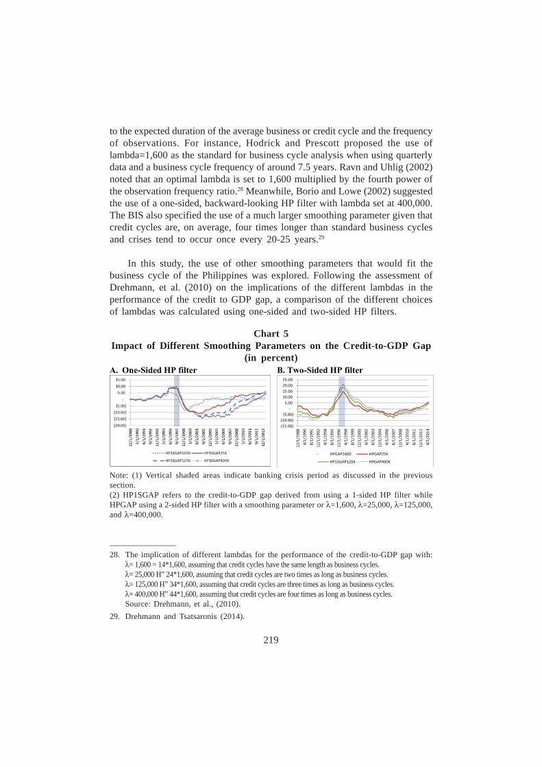
In this study, the use of other smoothing parameters that would fit thebusiness cycle of the Philippines was explored. Following the assessment ofDrehmann, et al. (2010) on the implications of the different lambdas in theperformance of the credit to GDP gap, a comparison of the different choicesof lambdas was calculated using one-sided and two-sided HP filters.

Chart 5Impact of Different Smoothing Parameters on the Credit-to-GDP Gap

(in percent)

Note: (1) Vertical shaded areas indicate banking crisis period as discussed in the previoussection.(2) HP1SGAP refers to the credit-to-GDP gap derived from using a 1-sided HP filter whileHPGAP using a 2-sided HP filter with a smoothing parameter or λ=1,600, λ=25,000, λ=125,000,and λ=400,000.

________________28. The implication of different lambdas for the performance of the credit-to-GDP gap with:

λ= 1,600 = 14*1,600, assuming that credit cycles have the same length as business cycles.λ= 25,000 H” 24*1,600, assuming that credit cycles are two times as long as business cycles.λ= 125,000 H” 34*1,600, assuming that credit cycles are three times as long as business cycles.λ= 400,000 H” 44*1,600, assuming that credit cycles are four times as long as business cycles.Source: Drehmann, et al., (2010).

29. Drehmann and Tsatsaronis (2014).

220

Chart 5 shows the time series of Philippine credit-to-GDP gap using lambdaof 1,600, 25,000, 125,000 and 400,000 under one- and two-sided HP filters. Byvisually inspecting gap movements around historical banking crisis, gaps withhigher lambdas of 400,000 and 125,000, in both one-sided and two-sided HPfilters, appear to have wider positive and negative gaps before and after a crisis.Eliminating the wider gaps, Chart 6 shows the less volatile credit-to-GDP gaptime series, in particular, using lambda of 25,000 both in one- and two-sided HPfilters.

5. Lag Length Determination

5.1 Credit-to-GDP Gap as an EWI for Banking Crises

Several empirical studies have already documented the ability of the credit-to-GDP gap to act as an EWI for banking crises. Drehmann and Tsatsaronis(2014), for instance, documented evidences when credit-to-GDP gap performsbest as EWI based on certain criteria proposed by Drehman and Juselius (2014).The study suggests that an EWI must be able to provide signals in advance forpolicy measures to take effect. In the BIS guidance, “the indicator should breachthe minimum critical threshold at least two to three years prior to a crisis.”Further, an EWI should be a stable indicator and should not signal periods withoutcrisis to reduce uncertainty in the variable which serves as basis for policymakersin their decision making. Finally, an EWI should be easy to interpret andunderstand for both the regulators and the financial institution.

In this study, the EWI property of the credit-to-GDP gap was examined bycomparing the gap series with the Philippine banking system’s indicator of financialdistress or the NPA. Chart 6 shows the ability of the gap as an EWI given thelead time of the indicator to turn positive several quarters before a run-up inbanks’ NPAs. In particular, the gap series, calculated by means of a one-sidedHP filter with a lambda of 25,000, shows a lead lag of 40 quarters or gapturning positive before NPA reached its peak in 1Q 2002. After the crisis, thegap fell rapidly and turned negative for 39 quarters from 3Q 1998 to 1Q 2008and turned positive again in 2Q 2008 and has consistently increased up to 2Q2014.

Relative to a two-sided HP filter using a similar smoothing parameter, thelead lag is 25 quarters or the period when gap turned positive and rose consistentlyuntil the gap reached its widest in 4Q 1997. The gap fell after the crisis andreached the negative territory after 15 quarters, in contrast to the series usingone-sided HP where the gap turned negative only in 6 quarters from its widest

221

in 4Q 1996. This may imply that using a one-sided HP filter, rather than the 2-sided HP, can give policymakers more time in announcing and implementingcapital buffer add-ons especially during the accumulation phase.30

Chart 6Comparison of 1- and 2-Sided HP Filter with l=25,000 and

Banks’ Non-Performing Assets (NPA)(Gap in percent, NPA in million pesos)

Note: HP1SGAP25K refers to the credit-to-GDP gap derived from usinga 1-sided HP filter while HPGAP25K using a 2-sided HP filter, both witha smoothing parameter or λ=25000.

To statistically assess if the key variable has the property of an EWI, alead-lag relationship between a banking indicator of stress and the gap serieswas conducted. The regression analysis between the growth in the bankingsystem’s NPA (dependent variable) and lagged values of the credit-to-GDP gap(independent variable) was estimated as described in equation 5.

NPA Growth = f(credit – to – GDP gap (–1 to – 20)) (5)

The results indicate a credit-to-GDP gap series with lag values of 8-10quarters register statistically significant relationship with NPA growth (see AnnexTable 5). A lag of 9 quarters has the highest coefficient and is statisticallysignificant at 99% probability and can explain about 25% of the changes in NPA

________________30. On this note, Drehmann and Tsatsaronis (2014) stressed that applying a 2-sided HP filter

may not be practical for policymakers since future values of the credit-to-GDP ratio isunobservable, reducing the signaling ability of the credit-to-GDP gap.

222

growth. This means that NPA is expected to reach its peak level in about 9quarters after the credit-to-GDP gap hit its highest point level, giving enoughtime for the policymakers to announce a potential accumulation of CCCB.

To further test the signaling ability of the choice variable, this study employeda signal extraction methodology in the assessment of the appropriate lambdavalues of the credit-to-GDP gap as the conditioning variable for CCCB. Kaminskyand Reinhart (1999) and Drehmann, et al. (2010) noted that an ideal indicatoris generally chosen by their ability to signal all impending crises and not thecrises that did not happen. The best indicator is chosen on the basis of thelowest noise-to-signal ratio (NTSR), or the fraction of Type II errors (a signalis issued but no crisis occurs) over 1 minus the fraction of Type I errors (nosignal is issued but a crisis occurs).This is represented by equation 6.

(6)

Where:

The equation also implies that the smaller the NTSR, the lower the noise.Using the same equation, the probability of an indicator correctly signaling acrisis is computed using equation 7.

P (crisis|signal) = (7)

The model assumes that a signal of 1 (0) is judged to be correct if a crisis(no crisis) occurs any time within a two-year horizon. A range of threshold forthe gap series using different lambda values 1,600, 25,000, 125,000, and 400,000are assessed. Annex Table 6 summarises the result of the NTSR test. Theanalysis shows that a gap series based on lambda of 25,000 has the smallestNTSR and satisfies the condition that at least two-thirds of crises are predictedwhen setting the threshold at 5.

Table 5True and False Crisis Signals

223

Further, using the same signaling extraction methodology employed in thecredit-to- GDP gap, Annex Table 7 shows the NTSR results for othermacroeconomic conditioning variables that are often used by literatures as EWIof financial crises. The results indicate that the credit-to-GDP gap still has thelowest NTSR and higher crisis predicted than other variables.

On the other hand, it is important to note that the conditioning variablesidentified should already signal a build-up in vulnerabilities 8 quarters or 2 yearsprior to the peak of a crisis. As stressed in the Drehman, et al. (2010) study,such signal will be counted as “false” despite the indicator providing a signalonly in advance. This increases the likelihood of a Type II error and a higherNSTR results, implying that no single variable can provide the perfect signal fora banking crisis. Hence, there is a need for constant discretion from the regulatorsin managing the timing and degree of a CCCB.

The empirical results from the analysis in Sections 4 and 5 propose the useof a credit-to-GDP gap as a conditioning variable in the adoption of a CCCBmetric in the Philippines. The choice of a 25,000 lambda in a one-sided HP filterappears to be the best smoothing parameter among the filter iterations performedas compared to the 400,000 specification suggested by the BIS.

As EWI for banking sector crises, the credit-to-GDP gap likewise showssignificant statistical performance given its low noise-to-signal ratio and the abilityto predict at least two-thirds of crises at a threshold of 5. Similarly, the variableexhibits a significant lag relationship with growth in NPA of the banking systemat a lag of 8-10 quarters. The credit-to-GDP gap as the choice variable givespolicymakers ample time in preparing banks especially for the accumulation phaseof the CCCB.

5.2 Sarel’s Methodology

The mechanical use of the credit-to-GDP gap as a common reference pointfor taking buffer decisions is constantly challenged in terms of its ability to actas a leading indicator of systemic banking crisis. In this section, the strength ofthe credit-to-GDP gap is tested further with regard to how it may relate to thebanking sector’s NPA at a particular threshold. The threshold level of the triggervariable was evaluated by using the model of Sarel (1996) which identifies therelationship of the growth in banking sector’s NPA (dependent variable) withthe credit-to-GDP gap and a threshold variable Xi. Equation 8 estimates theregression:

224

GrowthNPA = f(Gap, Xi) (8)

Where:

Variable (Xi) = Credit-to-GDP gap * DummyDummy Variable = Credit-to-GDP gap > ThresholdThreshold = 0-9

Annex Table 8 summarises the results of the regression. It showed that thecredit-to-GDP gap and the Xi variables are positively and significantly relatedwith the growth in NPA given p-values at 0 and t-statistics of above 3. The bestthreshold that can explain the growth in NPA is at level 5 with the highestcoefficient of 12.5 and lowest AIC of 8.1.

5.3 Calibration of Thresholds

The BIS guidelines set the thresholds, i.e., gap level L and gap level H, thatdetermine when the buffer is turned “on” and “off.” The gap level L is thethreshold which indicates that banks should start building up their capital buffers.The gap level H is when the buffer is at its maximum, i.e., the point that shouldbe reached before the onset of a crisis. At this level, no additional capital willbe required even if the gap will continue to increase.

As such, L should be low enough so that the banks are able to build upcapital in gradual fashion before the potential crisis. Banks are given one yearto raise additional capital which means that the indicator should breach theminimum at least 2-3 years prior to a crisis. In addition, L should be high enoughso that it will not be breached during normal times when no additional capitalis required. On the other hand, H should be low enough so that the capitalbuffer will be fully complied with before a major banking crisis.

In the case of the Philippines, the NTSR robustness test showed a thresholdsignificant at level 5 while results of the Sarel’s methodology suggest a thresholdof 5 to 6. If L should be low enough to give banks ample time to build up buffersand high enough so that the capital buffer may not be triggered in the absenceof a crisis, an L equal to 4 or 5 can be considered. Meanwhile, in determiningthe upper bound threshold H, the BIS guidelines recommend an “L+8” rule.With L set at 4-5, the H can be set at around 12-13.

225

Chart 7Credit to GDP Gap and Buffer

(in percent, L=4 H=12)

Note: Gap1s25K refers to the credit-to-GDP gap derived from using a 1-sidedHP filter with a smoothing parameter or λ=25000.

Given the above results, the lower threshold L, or the period when thebuffer guide will start to indicate the need to build up capital can be set at 4while the maximum H, at which the point where no additional capital is requiredeven if the gap will continue to increase, can be set at 12. With L=4 and H=12,the buffer guide is turned “on” 12 quarters or 3 years prior to 4Q 1997, justenough time for authorities to announce and implement the accumulation phaseof a CCCB. The buffer hit its highest level of 1.5% in 3Q 1997 when the gapis at its maximum. Further, the buffer declined immediately after the peak level,signaling the release phase which requires the reduction in the buffer to takeeffect at once to help reduce the risk of a contraction in the supply of creditas previously constrained by the buffer measure. In contrast with the resultsusing the BIS framework, the buffer was turned “on” 18 quarters prior to thepeak of the crisis which indicate that L=2 may be too low and translates to anearlier-than-recommended trigger when banks are supposed to start building upbuffers.

Moreover, the calibrated threshold points to a build-up in buffer beginning3Q 2011 and is set “on” in the next 12 quarters up to 2Q 2014. The buffer build-up is triggered by the increase in the credit-to-GDP gap brought about by highergrowth in private domestic credit which started to register at a double digit rateof 15.4%. It is noted that during this period, the Philippines did not experiencea banking crisis, although was not totally immune from the external headwinds

226

of the global financial crisis. The impact was largely through higher volatility inthe financial markets, causing large fluctuations in domestic asset prices.

5.4 Buffer Level and Progression

The previous sections focused on the timing of the build-up and release ofcapital buffers in a CCCB model. However, the indicators do not necessarilyindicate the optimal level of a countercyclical buffer. The above results werebased on a maximum buffer add-on set at 2.5% of bank’s risk weighted assets.When the credit-to-GDP ratio exceeds its long-term trend by 12 percentagepoints or more, the buffer add-on will be 2.5% of risk weighted assets. Whenthe credit-to-GDP ratio is four-percentage points or less its long-term trend, thebuffer add-on will be 0%. When the credit-to-GDP ratio is between four and12 percentage points of its trend, the buffer add-on will vary linearly between0 and 2.5%.

It maybe recalled that the aim of a CCCB is to ensure that banks havesufficient capital in such a way that they can operate efficiently during periodsof stress without limiting the supply of credit in the economy. Hence, it is importantto identify the period where required capital is expected to fall in a stressedsituation and the corresponding impact of the additional capital requirment oneconomic activity during normal times. The size of the buffer may depend onthe amount of expected losses that banks may incur in periods of financial stress.In identifying the optimal level of the buffer guide, the use of stress testing toolscan be employed or by directly examining the losses incurred by banks in pastcrises periods.31

In the case of the Philippines, the results from the previous exercise showthat the maximum buffer reached was only at 1.5%. There may be a need tore-assess the application of a 2.5% buffer add-on for a CCCB. A lower bufferamount can be examined in terms of its applicability in the local banking system.There may be country-specific factors that warrant an optimal capital bufferamount which can efficiently balance the cost of higher capital requirements oneconomic growth in non-crisis times as well as the benefit of easing the requiredcapital in periods of financial stress.

________________31. ibid., Riksbank, p.31.

227

6. Release Phase

The BIS was clear about the need to assess a broad range of indicatorsin taking decisions on buffer. The authorities should be mindful of how the choicevariable moves with other factors especially in taking buffer decision both in thebuild-up and release phase.

For instance, Drehman, et al. (2010) noted that the credit-to-GDP ratio andcredit growth indicators may perform well in anticipating crises as both variablesincrease consistently well above the trend before a crisis period but fall too lateand too slow especially during the onset of a crisis. If used in the release phaseof a CCCB, the timing can be late and the timing of the release may not beas immediate as what is required. Moreover, deviations of the property priceindicators were also found to be helpful in the build-up phase but not in therelease phase as difference from its long-term trend tends to narrow before acrisis emerge which can prompt an early release of the buffer. This can runcounter to what a CCCB aims to achieve, in particular, in reducing the risk ofcontracting the supply of credit in crisis time by promptly reducing the amountof buffer during this period.

In the same paper, high-frequency financial variables such as credit spreadsindicated strength in their usefulness as indicators for the release phase of aCCCB. These variables tend to perform well in a crisis period, rising faster asstrains emerge after staying below their long-term average in normal times.They are good in capturing the current level of stress in the financial sector butless useful in signaling an impending crisis since they reflect the materialisationof risks rather than its build-up.32

Countercyclical buffer decisions should not only depend on the choiceindicators such as the GAP ratio or credit growth variables. As reflected in theprevious section, the credit-to-GDP gap alone was unable to fully anticipate acrisis from happening. The low R-squared values of around 20-25% reflect thatthe credit gap series can explain only a portion of the changes in banks’ NPA.In addition, the gaps remained high even after the crisis which could affect thetiming of the release of the buffer.

________________32. ibid., Riksbank, p.21.

228

6.1 Supplementary Indicators

In this section, a number of supplementary indicators are examined in termsof their ability to signal in the release phase of the buffer. A simple correlationbetween the NPA growth and the lag of selected macroeconomic and financialmarket indicators was conducted. Annex Table 9 presents the correlationcoefficients, t-statistics, and p-values between the main variables in our model.The results show that NPA growth and changes in residential capital values hasthe highest correlation coefficient and is significant at a lag of 1. Meanwhile,significant correlation between growth in NPA and growth in stock market returnsis highest at lag 2. The negative and significant correlation between NPA growthand growth in capital land values and stock market return may imply a wealtheffect that negatively impacts the collateral channel such that when growth incapital values and stock market returns decline, growth of banks’ NPA increases.

As an indicator of financial stress, the results show that the identified variablescan be useful indicators in the release phase of the buffer as these variablestend to signal one or two quarters ahead of NPA. On the other hand, thecorrelation between NPA growth and real credit growth is significant at lag 8which reflects the strength of the variable as an early warning indicator and notas indicator in the release phase.

With the indicators identified, the next step will be to look at the modalitiesin the release of the buffer, i.e., immediate or gradual drawdowns. A buffershould be released if various stress indicators are signaling a high level of stresson the financial sector. The BIS noted that the release should be in periodswhen banks are already incurring losses such that the buffer is depleted firstbefore banks begin tapping their normal capital conservation buffer. If a bufferis released before losses have been incurred, there is a risk that the extra capitalcan be used to pay out dividends instead of lending it out. The release shouldbe timely to allow banks to use the capital and thereby lessen the potential riskof a credit crunch. It is therefore important for regulators to be clear about thepurpose of the buffer release in order to identify the appropriate modalities ineasing buffer restrictions, which can be a choice between absorbing losses orin maintaining credit flow in the system. This study recommends a further analysison this matter.

6.2 Communication

The need to pre-announce buffer requirements with a lead time of two tothree years to give banks ample time to adjust their capital position warrants the

229

development of an appropriate communication strategy from the regulators. TheBIS stressed the necessity of communicating buffer decisions in a timely mannerto promote accountability from the regulators and sound decision making fromfinancial institutions. In the build-up phase, planning the timing of the announcementcan help reduce the risk of the buffer not being in place before the credit cycleturns. In the release phase, communicating the immediate deactivation of thebuffer is essential so as not to contract the supply of credit in periods whenbanks needed the reprieve the most.

Since there are limited number of central banks that have already adoptedthe measure and with most of these banks from advanced economies, there isa need to design a communication plan that can work for economies like thePhilippines. This should be aligned with the appropriate analytical tools that allowfor an efficient announcement of an entry and exit decision by regulators. Thecommunication strategy should form part of regulator’s periodic assessment ofmacroeconomic and financial condition to determine whether the CCCB shouldbe activated, adjusted or turned off. Pronouncements should be reviewed andupdated on a regular basis so that any changes in the authorities’ outlook canbe publicly announced in a timely manner. This can help smoothen out theexpectations and give banks enough time to adjust and plan their capital positions.The BIS suggests that the authorities should revisit and comment on potentialchanges and updates in the model at least once a year using the variouscommunication tools available.

Should the Philippines implement a CCCB, the assessment as well as theannouncement can form part of the BSP’s Financial Stability Report (FSR).33

With the FSR providing a comprehensive assessment of the robustness as wellas vulnerabilities of the domestic financial system against the emerging economicand financial developments both in the global and domestic environment, theassessment for the build-up and release of a CCCB can leverage from theresults of the FSR report.

The semi-annual frequency of the publication of the FSR by the BSP willkeep the market well informed with regard to the developments of financialrisks and exposures that can potentially impact the overall stability and efficiencyof the economy which can subsequently trigger the activation of additional capitalbuffer. Overall, communicating CCCB decisions through the FSR will help: 1)

________________33. As of writing, the FSR is published by the BSP internally since 2007.

230

improve the understanding of risks to financial intermediaries in the economy;2) alert financial institutions and market participants on the possible collectiveimpact of their individual actions/decisions; and 3) build a consensus for financialstability and the improvement of the financial and regulatory infrastructure.34

7. Consensus, Recommendations and Conclusions

The study aims to arrive at a consensus in terms of finding the appropriateindicator to be used in the establishment of a CCCB in SEACEN membereconomies. For the Philippines, the empirical results suggest the use of the credit-to-GDP gap as a choice variable in taking buffer decisions especially in thebuild-up phase of a CCCB. The study highlights the ability of the GAP seriesto signal a financial stress event compared with other variables such as creditgrowth, GDP growth, stock market returns, and changes in residential capitalvalues.

With the credit-to-GDP gap as a choice variable, the calculation of a rule-based CCCB guide using the BIS framework showed the need to recalibratesome assumptions that will best fit the Philippine credit cycle. The results of thefilter iteration exercises in establishing the trend of the GAP series showed thata lower smoothing parameter or a lambda equal to 25,000 using a one-sided HPfilter can best capture stress events in the domestic financial system. In examiningthe strength of the variable as an EWI, the results of the stepwise regressionindicate a credit-to-GDP gap series with lag values of 8-10 quarters registerstatistically significant relationship with NPA growth. This means that NPA isexpected to reach its peak level in about 2.5 years after the credit-to-GDP gaphit its highest level, giving enough time for the policymakers to announce apotential accumulation of the CCCB. In selecting threshold levels that shouldtrigger the build-up phase of the buffer, the results of the robustness tests onthe basis of the lowest noise-to-signal ratio and from Sarel’s method of total fitsuggest the use of a lower and upper bound thresholds of 4 and 12, respectively,different from the L=2 and H=10 thresholds proposed by the BIS.

The study also highlights that countercyclical buffer decisions should notonly depend on a single choice indicator such as the GAP ratio or credit growthvariables. In this study, the correlation analysis of supplementary indicators andbanks’ NPA suggest that high frequency financial variables such as growth in

________________34. 2013 BSP Financial Stability Report.

231

stock market returns and changes in capital land values can be useful indicatorsin the release phase of the buffer as these variables peak one or two quartersahead of NPA. On the other hand, since these are just two of the financialmarket data available, there may be a need to examine further other quantitativeand qualitative indicators of banks’ risk taking behaviour such as banks’ creditdefault swaps and financial stability index as supplementary indicators in therelease phase of the buffer.

On the other hand, the study raises some issues in the conduct of a CCCBmeasure in the Philippines. First, the guide may be successful in “predicting” theAsian financial crisis and in signaling the appropriate buffers amount but this isonly one event. There may be a need to lengthen the series of the choice variablesto capture other banking crisis and the development of the choice variablesduring these events. Second, while the study focused on identifying the timingof the build up and release of capital buffers in a CCCB model, the indicatorsdo not necessarily reflect the optimal level of a countercyclical buffer. Theremay be a need to re-assess the 2.5% maximum buffer add-on as suggested bythe BIS. There can be country-specific factors that warrant an optimal capitalbuffer amount which can efficiently balance the cost of higher capitalrequirements on economic growth in non-crisis times as well as the benefit oflower capital in periods of financial stress. Finally, there is a need to developan appropriate communication strategy should regulators start to implement aCCCB. Since there are limited number of central banks that have already adoptedthe measure and with most of these banks coming from advanced economies,there is a need to design a communication plan that can work for economieslike the Philippines. This should be aligned with the appropriate analytical toolsthat allow for an efficient announcement of the entry and exit decisions byregulators.

232

References

Association of Financial Markets in Europe, (AFME), “Countercyclical CapitalBuffers Limiting Procyclicality,” Available at: <http//www/afme.eu/WorkArea/DownloadAsset.aspx?id=118>.

Bangko Sentral ng Philipinas, (2013), “Basel III Implementation in the Philippines,”Box Article 4, Bangko Sentral ng Philipinas Annual Report 2013.

Basel Committee on Banking Supervision, (2010), “Basel III: A Global RegulatoryFramework for More Resilient Banks and Banking System,” December,Rev. June 2011.

Basel Committee on Banking Supervision, (2009), “Comprehensive Response tothe Global Banking Crisis,” Bank of International Settlements, PressRelease: 7 September.

Basel Committee on Banking Supervision, (2010), “Guidance for NationalAuthorities Operating the Countercyclical Capital Buffer,” Bank ofInternational Settlements, December.

Borio, C.; C. Furfine; and P. Lowe, (2001), “Procyclicality of the Financial Systemand Financial Stability: Issues and Policy Options,” Bank of InternationalSettlements Paper, No. 1.

Chen, D. X. and I. Christensen, (2010), “The Countercyclical Bank Capital Buffer:Insights for Canada,” Bank of Canada Financial System Review.

Drehmann, M.; C. Borio; and K. Tsatsaronis, (2012), “Characterising the FinancialCycles: Don’t Lose Sight of the Medium Term,” BIS Working Papers,No. 380.

Drehmann, M.; C. Borio; L. Gambacorta; G. Jimenez and C. Trucharte, (2010),“Countercyclical Capital Buffers: Exploring Options,” BIS Working Paper,No. 317, July.

Drehmann, M. and K. Tsatsaronis, (2014), “The Credit-to-GDP Gap andCountercyclical Capital Buffers: Questions and Answers,” Bank ofInternational Settlement Quarterly Review, March.

233

Floro, D., (2010), “Loan Loss Provisioning and the Business Cycle: Does CapitalMatter? Evidence from Philippine Banks,” BIS Working Paper.

Gochoco-Bautista, M. S., (1999), The Past Performance of the Philippine BankingSector and Challenges in the Post-crisis Period.

KPMG, (2011), Basel III: Issues and Implications.

Leitner, S., (2005), “The Business Cycles in the Philippines: A Characterisation,”Philippine Management Review, Vol. 12, pp. 9-22.

Morgan, P. and V. Pontines, (2013), “An Asian Perspective on Global FinancialReforms,” Asian Development Bank Working Paper, No 433.

Misina, M. and G. Tkacz, (2009), “Credit, Asset Price, and Financial Stress,”International Journal of Central Banking, Vol. 5, No. 4.

Packer, F. and H. Zhu, (2012), “Loan Loss Provisioning Practices of AsianBanks,” BIS Working Papers, No. 375.

Parcon-Santos, H. and E. Bernabe, (2012), “The Macroeconomic Effects ofBasel III Implementation in the Philippines: A Preliminary Assessment,”Bangko Sentral ng Pilipinas Working Paper Series, No. 2012-02.

Pouvelle, C., (2012), “Bank Credit, Asset Prices, and Financial Stability: Evidencefrom French Banks,” IMF Working Paper, No. WP/12/103.

Repullo, R. and J. Saurina, (2011), “The Countercyclical Capital Buffer of BaselIII: A Critical Assessment,” CEMFI Working Paper, No. 1102.

Sveriges Riksbank, (2012), “Countercyclical Capital Buffers as a MacroprudentialInstrument,” Sveriges Riksbank Studies, December.

234

Annex Table 3 Descriptive Statistics

Annex Table 2 CCCB Policy Progress in the Philippines

Appendices

Annex Table 1 Characteristics of the Banking Sector in the Philippines

235

Annex Table 6Comparison of Different Choices of the Credit-to-GDP Gap Lambda Values

Annex Table 5 Regression Results of Credit-to-GDP gap and NPA growth

(Gap using 1-Sided HP Filter with l=25,000)

Annex Table 4Summary Findings for the Philippines

Note: NPA growth is the dependent variable and credit to GDP gap as independentvariable

236

Annex Table 9 Correlation Coefficient of Selected Variables

Annex Table 8 Summary of Regression Results

Annex Table 7 Comparison of Macroeconomic Conditioning Variables

Note: X5 is the interactive dummy variable with thresold level equals 5.

*** Significant at the threshold of 1%, ** at 5%, * at 10%.Growth in residential capital land values and credit are in real terms.

237

Annex 10Using Other Conditioning Variables

The BIS guidance framework posted a caveat on the use of credit-to-GDPgap as the common reference in operating a CCCB, noting that “the guide doesnot always work well in all jurisdictions.” Many authors have proposed the useof indicators other than the credit-to-GDP gap as anchor variable.

Drehmann and Tsatsaronis (2014) compared the performance of sixindicators, which include the credit-to-GDP gap, credit growth, GDP growth,residential property price growth, debt service ratio, and non-core liability ratio.The indicators were assessed in terms of their strength as an early warningindicator (EWI) for banking crisis. The results showed that the credit-to-GDPgap is statistically the best single EWI indicator for forecast horizon betweenfive and two years.

Meanwhile, Repullo and Saurina (2011) proposed the use of real creditgrowth, or the deviations of credit growth with respect to its long-run average,as the common reference variable for taking buffer decisions. The study showedthat real credit growth appears to be a good signaling variable in the build-upof systemic risk and does not exacerbate the underlying procyclicality of Basel’sminimum capital requirements.

In this study, the use of real credit growth as an alternative conditioningvariable for the CCCB was also examined. The GDP deflator was used to getthe real credit from the existing nominal values. Chart 6 shows the series of realprivate sector credit with respect to the country’s GDP growth. The dotted lineshows credit for the period 4Q 1989 to 1Q 2014 and exhibits peak levels in 4Q1996, 3Q 2008, and 3Q 2013 while showing negative values in 3Q 1991, 4Q1998, 2Q 2002, and 2Q 2006. The solid line represents real GDP growth. Thechart reflects the positive correlation between the two variables with real creditgrowth lagging behind GDP growth in two periods, in 3Q 2008 and in 2Q 2010.

238

Chart 8 Real Private Sector Credit versus GDP growth

(in percent)

When compared against a banking sector variable or the NPA, Chart 7shows that the real credit growth peaked in 4Q 1996 which represents a lag of8 quarters prior to 3Q 1998 when NPA reached its highest growth. However,the relationship weakened after the crisis as the growth in NPA deceleratedwhile the growth in real credit exhibited a rising trend. The weakening abilityof the indicator to act as a signaling variable for a banking sector crisis couldbe a result of the series of regulatory and prudential measures implemented bythe BSP after the crisis that resulted in improvements in the banking system’sasset quality (i.e., lower NPAs amid rising growth in credit).

Chart 9 Real Private Sector Credit versus NPA growth

(in percent)