Embed Size (px)
Citation preview

©Goodwin, Graebe, Salgado, Prentice Hall 2000Chapter 6
Chapter 6
Classical PID ControlClassical PID Control

©Goodwin, Graebe, Salgado, Prentice Hall 2000Chapter 6
This chapter examines a particular control structurethat has become almost universally used in industrialcontrol. It is based on a particular fixed structurecontroller family, the so-called PID controllerfamily. These controllers have proven to be robustand extremely beneficial in the control of manyimportant applications.
PID stands for: P (Proportional)I (Integral)D (Derivative)

©Goodwin, Graebe, Salgado, Prentice Hall 2000Chapter 6
Historical NoteEarly feedback control devices implicitly orexplicitly used the ideas of proportional, integral andderivative action in their structures. However, it wasprobably not until Minorsky’s work on ship steering*
published in 1922, that rigorous theoreticalconsideration was given to PID control.This was the first mathematical treatment of the typeof controller that is now used to control almost allindustrial processes.
* Minorsky (1922) “Directional stability of automatically steered bodies”, J. Am. Soc. Naval Eng., 34, p.284.

©Goodwin, Graebe, Salgado, Prentice Hall 2000Chapter 6
The Current Situation
Despite the abundance of sophisticated tools, includingadvanced controllers, the Proportional, Integral,Derivative (PID controller) is still the most widelyused in modern industry, controlling more that 95% ofclosed-loop industrial processes*
* Åström K.J. & Hägglund T.H. 1995, “New tuning methods for PIDcontrollers”, Proc. 3rd European Control Conference, p.2456-62; andYamamoto & Hashimoto 1991, “Present status and future needs: The viewfrom Japanese industry”, Chemical Process Control, CPCIV, Proc. 4th Inter-national Conference on Chemical Process Control, Texas, p.1-28.

©Goodwin, Graebe, Salgado, Prentice Hall 2000Chapter 6
PID Structure
Consider the simple SISO control loop shown inFigure 6.1:
Figure 6.1: Basic feedback control loop
C(s)R(s) E(s) Y (s)U(s)
−+Plant
©Goodwin, Graebe, Salgado, Prentice Hall 2000Chapter 6
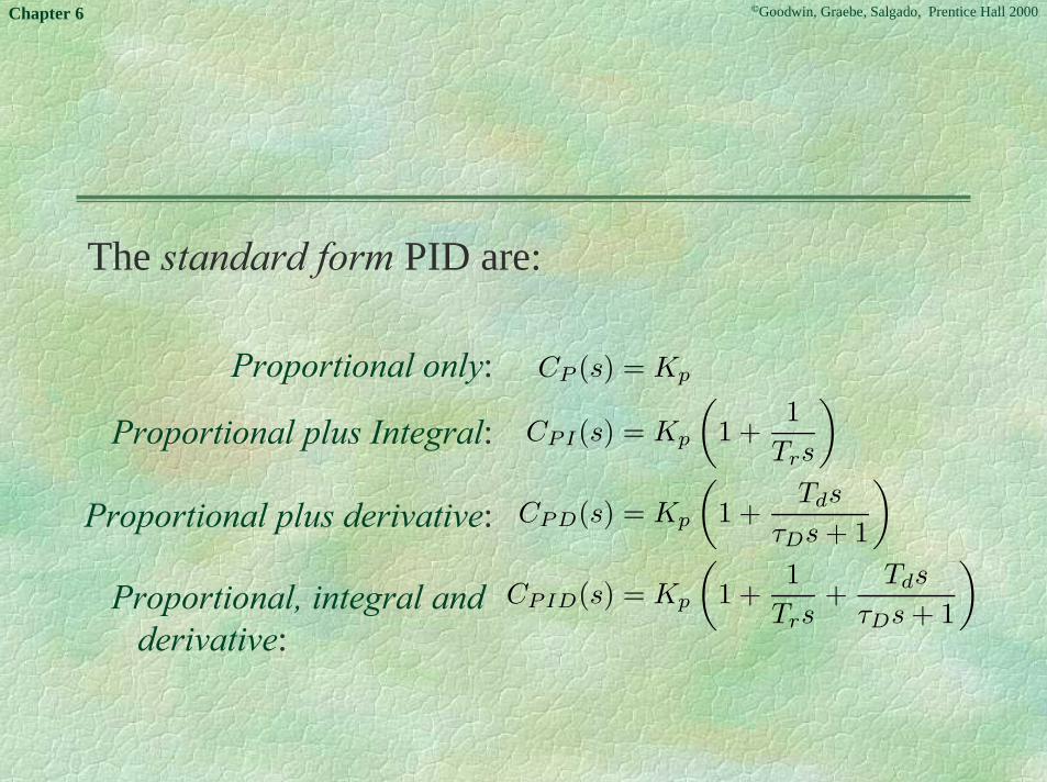
The standard form PID are:
CP (s) = Kp
CPI(s) = Kp
(1 +
1Trs
)
CPD(s) = Kp
(1 +
Tds
τDs + 1
)
CPID(s) = Kp
(1 +
1Trs
+Tds
τDs + 1
)
Proportional only:
Proportional plus Integral:
Proportional plus derivative:
Proportional, integral and derivative:

©Goodwin, Graebe, Salgado, Prentice Hall 2000Chapter 6
An alternative series form is:
Cseries(s) = Ks
(1 +
Is
s
) (1 +
Dss
γsDss + 1
)
Yet another alternative form is the, so called,parallel form:
Cparallel(s) = Kp +Ip
s+
Dps
γpDps + 1
©Goodwin, Graebe, Salgado, Prentice Hall 2000Chapter 6
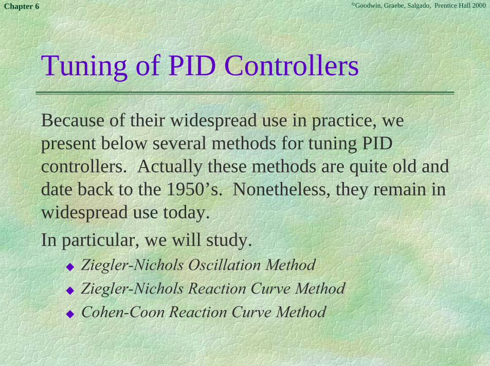
Tuning of PID Controllers
Because of their widespread use in practice, wepresent below several methods for tuning PIDcontrollers. Actually these methods are quite old anddate back to the 1950’s. Nonetheless, they remain inwidespread use today.In particular, we will study.
◆ Ziegler-Nichols Oscillation Method◆ Ziegler-Nichols Reaction Curve Method◆ Cohen-Coon Reaction Curve Method

©Goodwin, Graebe, Salgado, Prentice Hall 2000Chapter 6
(1) Ziegler-Nichols (Z-N) Oscillation Method
This procedure is only valid for open loop stableplants and it is carried out through the followingsteps
◆ Set the true plant under proportional control, with avery small gain.
◆ Increase the gain until the loop starts oscillating. Notethat linear oscillation is required and that it should bedetected at the controller output.

©Goodwin, Graebe, Salgado, Prentice Hall 2000Chapter 6
◆ Record the controller critical gain Kp = Kc and theoscillation period of the controller output, Pc.
◆ Adjust the controller parameters according to Table6.1 (next slide); there is some controversy regardingthe PID parameterization for which the Z-N methodwas developed, but the version described here is, to thebest knowledge of the authors, applicable to theparameterization of standard form PID.

©Goodwin, Graebe, Salgado, Prentice Hall 2000Chapter 6
Table 6.1: Ziegler-Nichols tuning using theoscillation method
Kp Tr Td
P 0.50Kc
PI 0.45KcPc
1.2PID 0.60Kc 0.5Pc
Pc
8

©Goodwin, Graebe, Salgado, Prentice Hall 2000Chapter 6
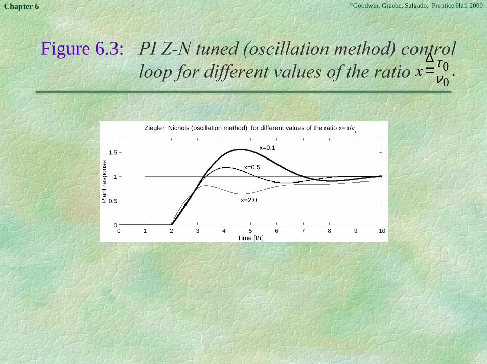
General System
If we consider a general plant of the form:
then one can obtain the PID settings via Ziegler-Nichols tuning for different values of τ and ν0. Thenext plot shows the resultant closed loop stepresponses as a function of the ratio
0;1)( 000
0 >+=−
γγτ
seKsG
s
.0ν
τ∆=x
©Goodwin, Graebe, Salgado, Prentice Hall 2000Chapter 6
Figure 6.3: PI Z-N tuned (oscillation method) controlloop for different values of the ratio .
00
ντ∆
=x
0 1 2 3 4 5 6 7 8 9 100
0.5
1
1.5
Time [t/τ]
Pla
nt r
espo
nse
Ziegler−Nichols (oscillation method) for different values of the ratio x= τ/νo
x=0.1
x=0.5
x=2.0

©Goodwin, Graebe, Salgado, Prentice Hall 2000Chapter 6
Numerical Example
Consider a plant with a model given by
Find the parameters of a PID controller using theZ-N oscillation method. Obtain a graph of theresponse to a unit step input reference and to a unitstep input disturbance.
Go(s) =1
(s + 1)3

©Goodwin, Graebe, Salgado, Prentice Hall 2000Chapter 6
Solution
Applying the procedure we find:
Kc = 8 and ωc = √3.
Hence, from Table 6.1, we have
The closed loop response to a unit step in thereference at t = 0 and a unit step disturbance at t = 10are shown in the next figure.
Kp = 0.6 ∗ Kc = 4.8; Tr = 0.5 ∗ Pc ≈ 1.81; Td = 0.125 ∗ Pc ≈ 0.45

©Goodwin, Graebe, Salgado, Prentice Hall 2000Chapter 6
Figure 6.4: Response to step reference and stepinput disturbance
0 2 4 6 8 10 12 14 16 18 200
0.5
1
1.5
Time [s]
Pla
nt o
utpu
t
PID control tuned with Z−N (oscillation method)

©Goodwin, Graebe, Salgado, Prentice Hall 2000Chapter 6
Different PID Structures?
A key issue when applying PID tuning rules (such asZiegler-Nichols settings) is that of which PIDstructure these settings are applied to.To obtain an appreciation of these differences weevaluate the PID control loop for the same plant inExample 6.1, but with the Z-N settings applied to theseries structure, i.e. in the notation used in (6.2.5),we have
Ks = 4.8 Is = 1.81 Ds = 0.45 γs = 0.1

©Goodwin, Graebe, Salgado, Prentice Hall 2000Chapter 6
Figure 6.5: PID Z-N settings applied to seriesstructure (thick line) and conventionalstructure (thin line)
0 2 4 6 8 10 12 14 16 18 200
0.5
1
1.5
2
Time [s]
Pla
nt o
utpu
t
Z−N tuning (oscillation method) with different PID structures

©Goodwin, Graebe, Salgado, Prentice Hall 2000Chapter 6
Observation
In the above example, it has not made muchdifference, to which form of PID the tuning rules areapplied. However, the reader is warned that this canmake a difference in general.

©Goodwin, Graebe, Salgado, Prentice Hall 2000Chapter 6
(2) Reaction Curve Based Methods
A linearized quantitative version of a simple plantcan be obtained with an open loop experiment, usingthe following procedure:
1. With the plant in open loop, take the plant manually to anormal operating point. Say that the plant output settles aty(t) = y0 for a constant plant input u(t) = u0.
2. At an initial time, t0, apply a step change to the plantinput, from u0 to u∞ (this should be in the range of 10 to20% of full scale).
Cont/...

©Goodwin, Graebe, Salgado, Prentice Hall 2000Chapter 6
3. Record the plant output until it settles to the new operatingpoint. Assume you obtain the curve shown on the nextslide. This curve is known as the process reaction curve.
In Figure 6.6, m.s.t. stands for maximum slope tangent.
4. Compute the parameter model as follows
Ko =y∞ − yo
u∞ − uo; τo = t1 − to; νo = t2 − t1

©Goodwin, Graebe, Salgado, Prentice Hall 2000Chapter 6
Figure 6.6: Plant step response
The suggested parameters are shown in Table 6.2.
Time (sec.)
y∞
yo
to t
1 t
2
m.s.t.

©Goodwin, Graebe, Salgado, Prentice Hall 2000Chapter 6
Table 6.2: Ziegler-Nichols tuning using the reactioncurve
Kp Tr Td
Pνo
Koτo
PI0.9νo
Koτo3τo
PID1.2νo
Koτo2τo 0.5τo

©Goodwin, Graebe, Salgado, Prentice Hall 2000Chapter 6
General System Revisited
Consider again the general plant:
The next slide shows the closed loop responsesresulting from Ziegler-Nichols Reaction Curvetuning for different values of
1)(00
0 +=−
seKsG
s
γτ
.0ν
τ∆=x

©Goodwin, Graebe, Salgado, Prentice Hall 2000Chapter 6
Figure 6.7: PI Z-N tuned (reaction curve method)control loop
0 5 10 150
0.5
1
1.5
2
Time [t/τ]
Pla
nt r
espo
nse
Ziegler−Nichols (reaction curve) for different values of the ratio x= τ/νo
x=0.1
x=0.5
x=2.0

©Goodwin, Graebe, Salgado, Prentice Hall 2000Chapter 6
Observation
We see from the previous slide that the Ziegler-Nichols reaction curve tuning method is verysensitive to the ratio of delay to time constant.

©Goodwin, Graebe, Salgado, Prentice Hall 2000Chapter 6
(3) Cohen-Coon Reaction CurveMethod
Cohen and Coon carried out further studies to findcontroller settings which, based on the same model,lead to a weaker dependence on the ratio of delay totime constant. Their suggested controller settingsare shown in Table 6.3:
Kp Tr Td
Pνo
Koτo
[1 +
τo
3νo
]
PIνo
Koτo
[0.9 +
τo
12νo
]τo[30νo + 3τo]
9νo + 20τo
PIDνo
Koτo
[43
+τo
4νo
]τo[32νo + 6τo]
13νo + 8τo
4τoνo
11νo + 2τo
Table 6.3: Cohen-Coon tuning using the reaction curve.

©Goodwin, Graebe, Salgado, Prentice Hall 2000Chapter 6
General System Revisited
Consider again the general plant:
The next slide shows the closed loop responsesresulting from Cohen-Coon Reaction Curve tuningfor different values of
1)(00
0 +=−
seKsG
s
γτ
.0ν
τ=x

©Goodwin, Graebe, Salgado, Prentice Hall 2000Chapter 6
Figure 6.8: PI Cohen-Coon tuned (reaction curvemethod) control loop
0 5 10 150
0.5
1
1.5
2
Time [t/τ]
Pla
nt r
espo
nse
Cohen−Coon (reaction curve) for different values of the ratio x= τ/νo
x=0.1
1.0
x=5.0

©Goodwin, Graebe, Salgado, Prentice Hall 2000Chapter 6
Lead-lag Compensators
Closely related to PID control is the idea of lead-lagcompensation. The transfer function of thesecompensators is of the form:
If τ1 > τ2, then this is a lead network and when τ1 < τ2,this is a lag network.
C(s) =τ1s + 1τ2s + 1

©Goodwin, Graebe, Salgado, Prentice Hall 2000Chapter 6
Figure 6.9: Approximate Bode diagrams for leadnetworks (τ1=10τ2)
ω
ω
π4
20[dB]
|C|dB
∠C(jω)
1τ2
10τ2
1τ1
110τ1

©Goodwin, Graebe, Salgado, Prentice Hall 2000Chapter 6
Observation
We see from the previous slide that the lead networkgives phase advance at ω = 1/τ1 without an increasein gain. Thus it plays a role similar to derivativeaction in PID.

©Goodwin, Graebe, Salgado, Prentice Hall 2000Chapter 6
Figure 6.10: Approximate Bode diagrams for lagnetworks (τ2=10τ1)
−π4
−20[dB]
ω
ω
|C|dB
∠C(jω)
1τ2
110τ2
1τ1
10τ1

©Goodwin, Graebe, Salgado, Prentice Hall 2000Chapter 6
Observation
We see from the previous slide that the lag networkgives low frequency gain increase. Thus it plays arole similar to integral action in PID.

©Goodwin, Graebe, Salgado, Prentice Hall 2000Chapter 6
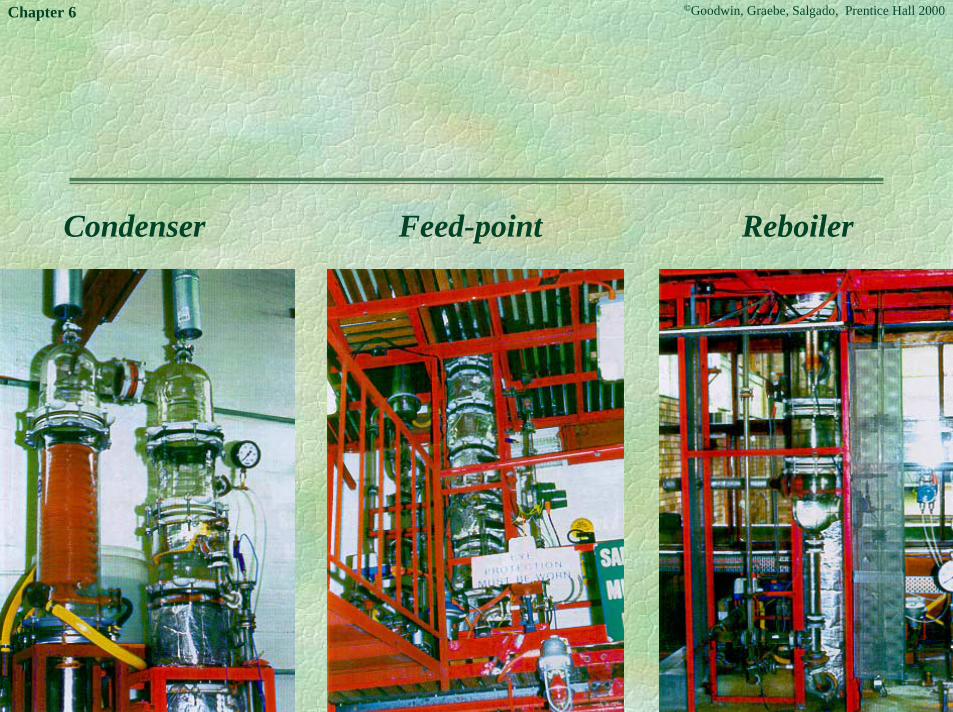
Illustrative Case Study: Distillation Column
PID control is very widely used in industry. Indeed,one would we hard pressed to find loops that do notuse some variant of this form of control.Here we illustrate how PID controllers can beutilized in a practical setting by briefly examiningthe problem of controlling a distillation column.

©Goodwin, Graebe, Salgado, Prentice Hall 2000Chapter 6
Example System
The specific system we study here is a pilot scaleethanol-water distillation column. Photos of thecolumn (which is in the Department of ChemicalEngineering at the University of Sydney, Australia)are shown on the next slide.
©Goodwin, Graebe, Salgado, Prentice Hall 2000Chapter 6
Condenser Feed-point Reboiler

©Goodwin, Graebe, Salgado, Prentice Hall 2000Chapter 6
Figure 6.11: Ethanol - water distillation column
A schematic diagram of the column is given below:

©Goodwin, Graebe, Salgado, Prentice Hall 2000Chapter 6
Model
A locally linearized model for this system is asfollows:
where
Note that the units of time here are minutes.
[Y1(s)Y2(s)
]=
[G11(s) G12(s)G21(s) G22(s)
] [U1(s)U2(s)
]
G11(s) =0.66e−2.6s
6.7s + 1
G12(s) =−0.0049e−s
9.06s + 1
G21(s) =−34.7e−9.2s
8.15s + 1
G22(s) =0.87(11.6s + 1)e−s
(3.89s + 1)(18.8s + 1)

©Goodwin, Graebe, Salgado, Prentice Hall 2000Chapter 6
Decentralized PID Design
We will use two PID controllers:
One connecting Y1 to U1
The other, connecting Y2 to U2 .

©Goodwin, Graebe, Salgado, Prentice Hall 2000Chapter 6
In designing the two PID controllers we will initiallyignore the two transfer functions G12 and G21. Thisleads to two separate (and non-interacting) SISOsystems. The resultant controllers are:
We see that these are of PI type.
C1(s) = 1 +0.25s
Cs(s) = 1 +0.15s

©Goodwin, Graebe, Salgado, Prentice Hall 2000Chapter 6
Simulations
We simulate the performance of the system with thetwo decentralized PID controllers. A two unit stepin reference 1 is applied at time t = 50 and a oneunit step is applied in reference 2 at time t = 250.The system was simulated with the true coupling(i.e. including G12 and G21). The results are shownon the next slide.

©Goodwin, Graebe, Salgado, Prentice Hall 2000Chapter 6
Figure 6.12:Simulation results for PI control ofdistillation column
It can be seen from the figure that the PID controllers give quite acceptableperformance on this problem. However, the figure also shows something that isvery common in practical applications - namely the two loops interact i.e. a changein reference r1 not only causes a change in y1 (as required) but also induces atransient in y2. Similarly a change in the reference r2 causes a change in y2 (asrequired) and also induces a change in y1. In this particular example, theseinteractions are probably sufficiently small to be acceptable. Thus, in commonwith the majority of industrial problems, we have found that two simple PID(actually PI in this case) controllers give quite acceptable performance for thisproblem. Later we will see how to design a full multivariable controller for thisproblem that accounts for the interaction.
0 50 100 150 200 250 300 350 400 450−1
−0.5
0
0.5
1
1.5
2
2.5
Pla
nt o
utpu
ts &
ref
.
Time [minutes]
r1(t)
y1(t)
r2(t)
y2(t)

©Goodwin, Graebe, Salgado, Prentice Hall 2000Chapter 6
Summary
❖ PI and PID controllers are widely used inindustrial control.
❖ From a modern perspective, a PID controller issimply a controller of (up to second order)containing an integrator. Historically, however,PID controllers were tuned in terms of their P, Iand D terms.
❖ It has been empirically found that the PIDstructure often has sufficient flexibility to yieldexcellent results in many applications.

©Goodwin, Graebe, Salgado, Prentice Hall 2000Chapter 6
❖ The basic term is the proportional term, P, whichcauses a corrective control actuation proportionalto the error.
❖ The integral term, I gives a correction proportionalto the integral of the error. This has the positivefeature of ultimately ensuring that sufficientcontrol effort is applied to reduce the trackingerror to zero. However, integral action tends tohave a destabilizing effect due to the increasedphase shift.

©Goodwin, Graebe, Salgado, Prentice Hall 2000Chapter 6
❖ The derivative term, D, gives a predictivecapability yielding a control action proportional tothe rate of change of the error. This tends to havea stabilizing effect but often leads to large controlmovements.
❖ Various empirical tuning methods can be used todetermine the PID parameters for a givenapplication. They should be considered as a firstguess in a search procedure.
©Goodwin, Graebe, Salgado, Prentice Hall 2000Chapter 6
❖ Attention should also be paid to the PID structure.
❖ Systematic model-based procedures for PIDcontrollers will be covered in later chapters.
❖ A controller structure that is closely related to PIDis a lead-lag network. The lead component actslike D and the lag acts like I.

©Goodwin, Graebe, Salgado, Prentice Hall 2000Chapter 6
Useful Sites
The following internet sites give valuableinformation about PLC’s:
www.plcs.net
www.plcopen.org
For example, the next slide lists the manufacturersquoted at the above sites.

©Goodwin, Graebe, Salgado, Prentice Hall 2000Chapter 6
ABBAlfa LavalAllen-BradleyALSTOM/CegelecAromatAutomation Direct/PLC Direct/Koyo/
B&R Industrial AutomationBerthel gmbh
Cegelec/ALSTROMControl MicrosystemsCouzet AutomatismesControl Technology CorporationCutler Hammer/IDT
Divelbiss
EBERLE gmbhElsag BaileyEntertron
Festo/Beck ElectronicFisher & PaykelFuji Electric
GE-FanucGould/ModiconGrayhillGroupe Schneider
Cont/�.

©Goodwin, Graebe, Salgado, Prentice Hall 2000Chapter 6
HimaHitachiHoneywellHorner Electric
IdecIDT/Cutler Hammer
Jetter gmbh
KeyenceKirchner SoftKlockner-MoellerKoyo/Automation Direct/PLC Direct
MicroconsultantsMitsubishiModicon/GouldMoore Products
OmronOpto22
PilzPLC Direct/Koyo/Automation Direct
RelianceRockwell AutomationRockwell Software
Cont/�.

©Goodwin, Graebe, Salgado, Prentice Hall 2000Chapter 6
SAIA-BurgessSchleicherSchneider AutomationSiemensSigmatekSoftPLC/Tele-DenkenSquare D
Tele-Denken/Soft PLCTelemecaniqueToshibaTriangle Research
Z-World

©Goodwin, Graebe, Salgado, Prentice Hall 2000Chapter 6
Additional Notes: Examplescommercially available PID controllersIn the next few slides we briefly describe some of thecommercially available PID controllers. There are, ofcourse, a great many such controllers. The examples wehave chosen are selected randomly to illustrate the kindsof things that are available.There are several variations in algorithms, with the threemain types being series, parallel and ideal form.Some controllers are configured to act on the error andsome apply the D term to the feedback only. Most havespecial features to deal with saturation and slew ratelimits on the plant input. (This topic is discussed inChapter 11).

©Goodwin, Graebe, Salgado, Prentice Hall 2000Chapter 6
Allen Bradley PLC-5 PID Block
The PID function in this controller is an outputinstruction that must be executed periodically atspecified intervals determined by the external code.

©Goodwin, Graebe, Salgado, Prentice Hall 2000Chapter 6
There are 4 different forms of the controller equation:
(1) With derivative action on the output
biasyeKus
sTsTc dT
di
+��
��
�
��
��
�
��
���
+
�
�� +=
+16111
(2) With derivative action in the error
biaseKus
sTsTc dT
di
+��
��
�
��
��
�
��
���
+
�
�� +=
+16111

©Goodwin, Graebe, Salgado, Prentice Hall 2000Chapter 6
(3) Similar to (1) but with different gains
biasyeKupKsdK
di sKs
Kp +
��
�
�
��
�
�
+���
��� +=
+161
(4) Similar to (2) but with different gains
biaseKupKsdK
di sKs
Kp +
��
�
�
��
�
�
++=+161

©Goodwin, Graebe, Salgado, Prentice Hall 2000Chapter 6
GEM 80 PIDABS Block
The GEM family of PLC’s have a PID block whichmust be executed periodically at specified intervalsdetermined by the external code. This function isimplemented by a velocity type algorithm, with thecontroller being converted to an absolute controllerby adding the previous output value. Thus thecontroller output is of the form:
( ) ( )100
2 2111
−−−−
+−++−+= tttctcttctt
eeeDeIeePuu

©Goodwin, Graebe, Salgado, Prentice Hall 2000Chapter 6
The reader can convert the above discreteimplementation to approximate continuous timeform by noting that
where ∆ is the sampling interval. Thus the controllaw is roughly equivalent to the following:
dtdett ee ≅∆
− −1
22
2212
dtedttt eee ≅
∆+− −−
���
��� ∆+∆+= esDeIsePsu c
cc
2100
1

©Goodwin, Graebe, Salgado, Prentice Hall 2000Chapter 6
Two comments regarding this equation are:
(1) Much more will be said on the relationshipbetween and and Chapters 12, 13and 14.
(2) Note that to achieve approximately the sameperformance with different sampling rates, Icand Dc need to be scaled.
∆− −= 1tt eeeδ dt
de

©Goodwin, Graebe, Salgado, Prentice Hall 2000Chapter 6
Yokogawa DCS Function Block
This DCS offers nine types of regulatory control blocks -◆ PID◆ Sampling PI◆ PID with batch switch◆ two position on/off controller◆ three position on/off controller◆ time proportioning on/off controller◆ PD with manual reset◆ blending PI◆ self tuning PID

©Goodwin, Graebe, Salgado, Prentice Hall 2000Chapter 6
The basic PID controller has 5 variations. The main3 structures being:
(1)
(2)
(3)
Note that the parameters in these controllers are(roughly) invariant w.r.t. ∆.
( ) ( )���
��
� +−∆+∆+−+= −−−− 2111 2 tttd
ti
ttpstt eeeTeTeeKKuu
( ) ( )���
��
� +−∆+∆+−+= −−−− 2111 2 tttd
ti
ttpstt yyyTeTeeKKuu
( ) ( )���
��
� +−∆+∆+−+= −−−− 2111 2 tttd
ti
ttpstt yyyTeTyyKKuu

©Goodwin, Graebe, Salgado, Prentice Hall 2000Chapter 6
Additional features of these controllers are◆ Selection of the type of equation, including the facility to invert the
output;◆ Automatic or manual mode selection, with an option for tracking;◆ Bumpless transfer;◆ Separate input and output limits, including rate and absolute limits;◆ Additional non-linear scaling of the output;◆ Integrator anti-windup (called reset-limiter);◆ Selectable execution interval as a multiple of scan time;◆ Feed forward, either to the feedback or controller output;◆ A dead-band on the controller output.

©Goodwin, Graebe, Salgado, Prentice Hall 2000Chapter 6
Fisher Controls 4195K GaugePressure Controller
This pressure controller is a pneumatic device, withmechanical linkages, that is coupled to a controlvalve, specifically for providing pressure regulation.One advantage of pneumatic controllers is that, asthey are powered by instrument air, there is noelectrical power employed.The controller can be configured as a P, PI or PIDcontroller, which can be configured as direct orreverse acting. Features such as anti-windup areoptional.