Chapter 6 Data Directed Importance Sampling for …ghuerta/papers/manuscript_v2_combined.pdf · Wiley STM / Editor: Advanced Computational Infrastructures for Parallel and Distributed

[Book Title], Edited by [Editor’s Name]. ISBN 0-471-XXXXX-X Copyright © 2000 Wiley[Imprint], Inc.

Chapter 6

Data Directed Importance Sampling for Climate Model Parameter Uncertainty Estimation

Charles S. Jackson1, Mrinal K. Sen1,2, Paul L. Stoffa1, and Gabriel Huerta3

1Institute for Geophysics, The University of Texas at Austin

2Department of Geological Sciences, The University of Texas at Austin

3Department of Statistics, University of New Mexico

Abstract Assessments of uncertainty in climate prediction require a meaningful ensemble of model

configurations that represent the limitation of observations to constrain arbitrary choices

in model formulation such as the values assigned to its multiple, non-linearly related

parameters. We present a data directed importance sampling strategy that makes optimal

use of distributed computing resources and improves the sampling efficiency over

uniform or random sampling strategies by several orders of magnitude. The algorithm is

then further developed to take into account uncertainties in our ability to establish a

Wiley STM / Editor: Advanced Computational Infrastructures for Parallel and Distributed Adaptive Applications, Chapter 6 / Authors Jackson, Sen, Stoffa, Huerta / filename: ch6.doc

page 2

normalized metric of model-data distance owing to the correlations that exist in space and

time among the 15 fields that are used to evaluate model skill. By incorporating estimates

of this uncertainty in the prior, further improvements can be attained in the accuracy and

efficiency of the stochastic sampling algorithm. The algorithm is then applied to

estimating an a posteriori probability density for 6 parameters important to clouds and

convection of the Community Atmosphere Model version 3.1. The top six performing

parameter sets improved model skill by 10% with nearly identical skill scores, but for

different reasons related to the wide range of selected parameter values. Efficiently

quantifying these uncertainties will provide important insights into the limitations of

climate model predictive skill within a time frame practical for climate model

development.

1. Introduction The 2001 Working Group I report from the Intergovernmental Panel on Climate Change

(IPCC, 2001) documents a wide disparity among existing models of the climate system in

their response to projected increases in atmospheric CO2 concentrations. Predictions of

global mean surface air temperature sensitivity to a doubling of atmospheric CO2

concentration (in ~100 years) range from ~2 to 6 degrees (LeTreut and McAvaney, 2000;

Cubasch et al., 2001). There are a number of possible reasons why these differences exist.

Although each climate model has been tuned to reproduce observational means, each

model contains slightly different choices of model parameter values as well as different

parameterizations of under-resolved physics (e.g. clouds, radiation, convection). Climate

model uncertainties are primarily estimated from model intercomparison projects (e.g.

Gates et al. 1999; Joussaume and Taylor 2000; Meehl et al., 2000; also see


page 3

www.clivar.org/science/mips.htm for a list of 31 ongoing projects). It is often assumed

that the range of behaviors exhibited by models that participate in the intercomparison

projects is representative of a realistic range of probable outcomes (e.g. Meehl et al.,

2000). Although there may be some recognition of which models perform better than

others, the qualitative approach to evaluating model performance does not lend itself to

assigning quantitative likelihoods to model predictions. The 2001 IPCC report, in its

assessment of current research needs, calls for “…a much more comprehensive and

systematic system of model analysis and diagnosis, and a Monte Carlo approach to model

uncertainties associated with parameterizations…” (Section 8.10, McAvaney et al.,

2001). The computational expense of typical atmosphere-ocean general circulation

models (AOGCMs) is a major barrier to reaching this goal. Two approaches have been

taken to address uncertainties arising from climate model parameters. One is based on a

reduced complexity climate model (Forest et al., 2000, 2001, 2002) and the other one

distributes the computational burden among thousands of under-utilized personal

computers (see www.climateprediction.net; Allen, 1999; Stainforth et al., 2005). Data

directed importance sampling for climate model parameter uncertainty estimation

concerns an improved framework for taking advantage of distributed computing

resources toward the goal of identifying multiple, non-linearly related parameter values

of a single climate model that reflect observational constraints on climate model

uncertainty. This goal is not trivial insofar as a single climate model experiment typically

uses a 30-year simulation or 1500 cpu hours to characterize a climate state and one may

need to complete millions of experiments to randomly sample all the potentially relevant

combinations of 10 or more parameter values.


page 4

Predictive uncertainty up to this point has been mainly associated with uncertainty in

CO2 emissions and/or natural variability, factors that may be treated in a fairly

straightforward manner. A far greater challenge is to represent the uncertainty that arises

from arbitrary differences in climate model parameter values when the parameters

themselves are non-linearly related (Kheshgi and White, 2001). This fact presents unique

challenges to those working to improve climate model predictions. One example of this

challenge became apparent within a presentation at the 2001 NCAR Community Climate

System Model (CCSM) Workshop in Breckenridge, Colorado. In an effort to improve

simulations of arctic climate, changes were made within the infrared radiation scheme to

make it more physical. This had the effect of improving the simulation of arctic climate

but at the expense of drying out the tropics. This was remedied in part by increasing the

amount of water that is allowed to evaporate from hydrometeors (rain drops) within

unsaturated downdrafts of convective clouds. In another particularly dramatic example,

Williams et al. (2001) document the effect of specific changes made in the process of

creating the next version of HadCM2 (Hadley Center Climate Model 2, United

Kingdom). The authors noticed that the response of precipitation over the tropical Pacific

to a doubling of atmospheric CO2 concentration within HadCM3 was entirely different

from the distribution found within HadCM2. The cause of these differences was found to

originate from the combined influence of small changes within two parameters affecting

mixing within the boundary layer and the critical humidity for cloud formation. Many of

these non-linear behaviors within models go unpublished, as the root causes are often

hard to identify and there often is not a strong link to any particular science question.


page 5

However, even these few examples underscore the need for a systematic approach for

evaluating climate model performance and a way to navigate through the seemingly

endless cycle of ‘educated guessing’ that now takes place each time a new version of a

climate model is released.

There are two useful objectives to an uncertainty analysis that considers how non-ideal

parameter value choices affect model predictions of climate. The first is to identify sets of

model parameter values that define members of an ensemble that is assured to be

representative of the combined uncertainty in the observations and model physics. The

second is the ability to identify an optimal set of parameter values that maximizes climate

model performance. As of yet, there has been little progress on meeting these objectives

outside of what can be gleaned from individual sensitivity experiments and model

intercomparison projects. The principal reason for this lack of progress is that most

traditional methods for meeting the first objective (e.g. Monte-Carlo or

Metropolis/Gibbs’ ‘importance sampling’) require 104 to 106 model evaluations

(experiments) for problems involving fewer than ten parameters.

Over the past decade, there has been significant progress within the mathematical

geophysics community for solving non-linear problems in geophysical inversion using

statistical methods to account for the possibility of multiple solutions (interpretations) of

geophysical data (for a review, see Barhen et al., 2000). Like climate models,

geophysical models are complex, computationally expensive, and involve many potential

degrees of freedom. Within the geophysics community, particular emphasis has been


page 6

placed on efficiency, although with some measured compromises. Similarly dramatic

advances have taken place within the statistics community over the past decade on a class

of methods of statistical inference known as Markov Chain Monte-Carlo (MCMC). In

particular, greater awareness now exists for how different challenges in robust statistical

inference can be addressed with Bayesian inference and sampling rules that obey the

properties of a Markov chain. In what follows we document progress being made on both

these fronts to advance the feasibility of quantifying climate model uncertainties that

stem from multiple, non-linearly related parameters.

Other, potentially useful approaches exist to estimating parameters and

uncertainties for complex systems. Examples include Latin-hypercube sampling and

kriging interpolation techniques to reduce the number of experiments that may be needed

to estimate the multidimensional dependencies (Sacks et al. 1989; Welch et al. 1992;

Bowman et al. 1993; Chapman et al. 1994; Santer et al., 2003). Within the climate

community, there has been some interest to apply the Ensemble Kalman Filter which uses

time trajectories of the climate system in much the same way traditional data assimilation

works in numerical weather prediction (e.g. Grell and Devenyi, 2002; Evensen, 2003;

Annan et al., 2007). This may provide another computationally feasible approach to the

tuning problem, but this approach still needs to prove its viability for the longer-term

climate problem. One concern is that many of the effects and feedbacks of model

parameter changes take time to express themselves. The parameter choices constrained

by short term weather would not be the same or ideally suited for a model meant for

predicting climate change (Lea et al., 2000). The point that will be developed below is

that estimates of the posterior distribution and optimization of model skill can be


page 7

performed through direct sampling, in parallel, with relatively few iterations and without

surface approximations.

2. Computing Climate Model Parameter Uncertainties in Parallel

The computation of parametric uncertainties in a climate model will take advantage of

two levels of parallelism; the parallelism of the climate model code and the parallelism

permitted by the stochastic sampler. In order to appreciate the advantages of the choice

of stochastic sampler it will be helpful to first document the computational characteristics

of the Community Atmosphere Model version 3.1 (CAM3.1) for which we are currently

testing the effects of 6 model parameters important to clouds and convection. CAM3.1

resolves the physics and fluid motions of the atmosphere on a 64 x 128 spectral grid with

26 vertical levels. For parallelism, the code exploits domain decomposition by the 64

latitude bands which place an effective upper limit on number of processors for which the

model can be run efficiently. The performance of CAM3.1 may be expressed by the

number of simulated years per wall clock day for a given number of processors. This

number may be normalized by the number of processors (years per day per processor) to

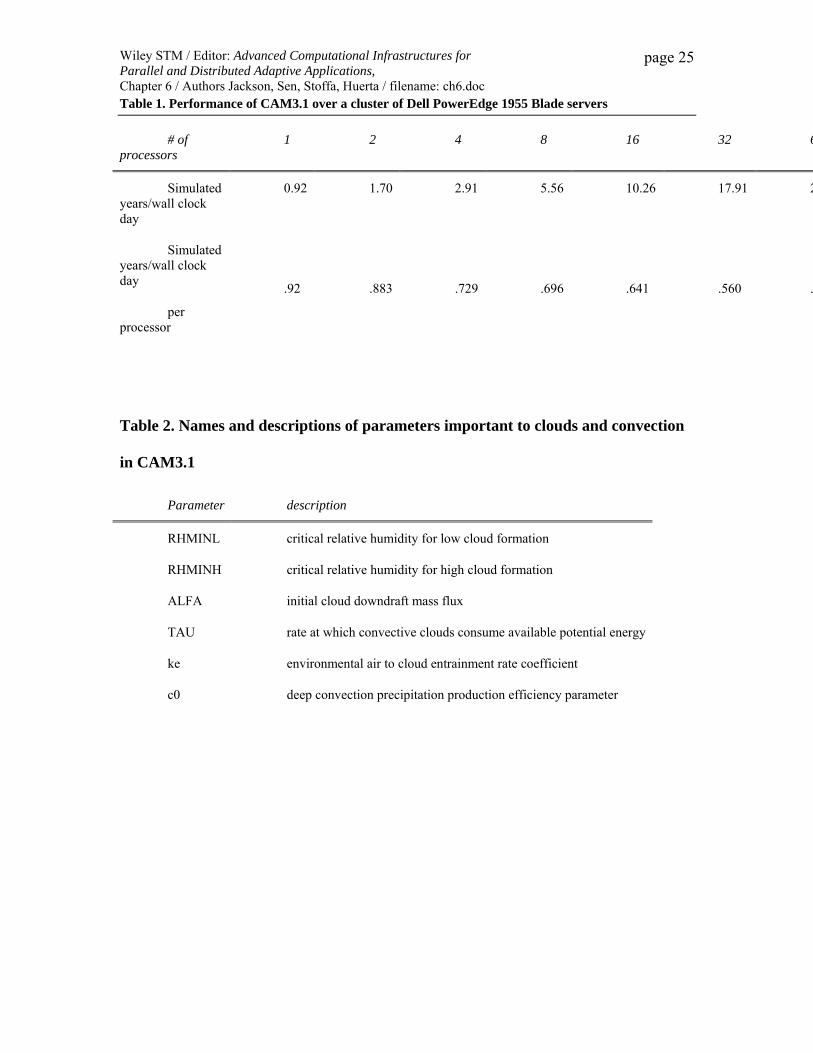
give a measure of the scaling efficiency of the code. Table 1 shows the performance of

CAM3.1 on a distributed computing platform available at the Texas Advanced

Computing Center. This platform consists of a distribution of Dell PowerEdge 1955

Blade servers each with dual socket/dual core 2.66 GHz Intel 64-Bit Xeon (Woodcrest)

processors and a 1333 MHz Front Side Bus and dual channel 533 MHz fully buffered

DIMMS. Each server is interconnected by an InfiniBand switch with a nominal

bandwidth of 1 Gigabit/s with 6µs latency, the overhead time for sending a packet of


page 8

information between any two processors. Climate models do not scale particularly well

within distributed computing environments because of the frequency at which

information needs to be shared among processors. This makes scaling performance

numbers more sensitive to latency numbers.

The performance numbers of table 1 provide a reality check on the enormity of the

problem to systematically evaluate all possible combinations of parameter values.

Without model parallelism, a single 10-year long experiment would take over a week. In

order to take advantage of the data-directed importance sampling described below, one

needs at least 150 of these experiments to be run sequentially. We therefore depend on

the model parallelism in addition to the stochastic sampling algorithm parallelism to

obtain scientifically relevant results within a reasonable time frame.

3. Stochastic Inversion Bayesian statistics uses rules of conditional probabilities to infer how a set of parameters

may be constrained by available observations given knowledge of a system’s physics.

The desired result is known as a posteriori probability density function (PPD). The PPD

is a powerful summary of information about how observational data can inform us about

key relationships of a physical system. The key to making this work efficiently is to allow

data to be involved in selecting candidate parameter values through a meaningful metric

of the distance between observations and model predictions. That is, the improved

efficiencies come from the process by which the choices of candidate parameter values

depend on past values. This dependency is not great news for application in distributed

computing environments as one wants to be completing as many experiments at once as


page 9

possible. Moreover, most algorithms for choosing candidate parameter values are not

terribly efficient, even when directed by data, and whatever efficiency they do achieve is

sensitive to characteristics of the shape of the likelihood function, the metric of model-

data discrepancies as a function of model parameters.

The optimal approach to stochastic inversion for data and/or computational demanding

problems is a subject of current research. One strategy that provides an adequate blend of

efficiency and accuracy is Multiple Very Fast Simulated Annealing (Sen and Stoffa,

1996; Jackson et al. 2004). The rules for selecting samples is similar to a

Metropolis/Gibbs sampler insofar as candidate parameter set values are either accepted or

rejected (for stepping through parameter space) in proportion to a probability

⎟⎠⎞

⎜⎝⎛ ∆−

=T

EP exp , (1)

where is the change in the metric of model-data discrepancies,

also called the “cost function”, for going from a model with parameter set values mk to

model with parameter set values mk+1. The mathematical form of E(m) is defined below.

The Metropolis/Gibbs sampler is sensitive to the algorithm “temperature” parameter T

which controls how freely the stochastic sampler will jump around parameter space. If

too high a temperature is selected, then the benefits of data-directed sampling are lost. If

too low a temperature is selected, then sampling will not be representative of the range of

possible solutions. Multiple Very Fast Simulated annealing avoids the ambiguity of

knowing in advance what the ideal temperature is by starting at a relatively high

temperature and allowing the stochastic sampler to experience a range of temperatures

according to the schedule in which iteration (k) has temperature

)()( 1 kk EEE mm −=∆ +


page 10

( )2/1)1(9.0exp −= kTT ok . (2)

The size of the steps that are taken through parameter space within MVFSA is connected

to temperature with larger steps at higher temperatures and smaller steps as T approaches

0. After a relatively few number of iterations, depending primarily on the dimensionality

of m, the MVFSA algorithm will converge on a solution that tends to favor the global

minimum of the cost function. The convergence process should be repeated 10 to 100s of

times to accumulate sufficient statistics to estimate the PPD. The advantage of MVFSA

for distributed computing is that the convergence attempt chains can be run in parallel

with the final estimate of the PPD coming from an accumulation of statistics across

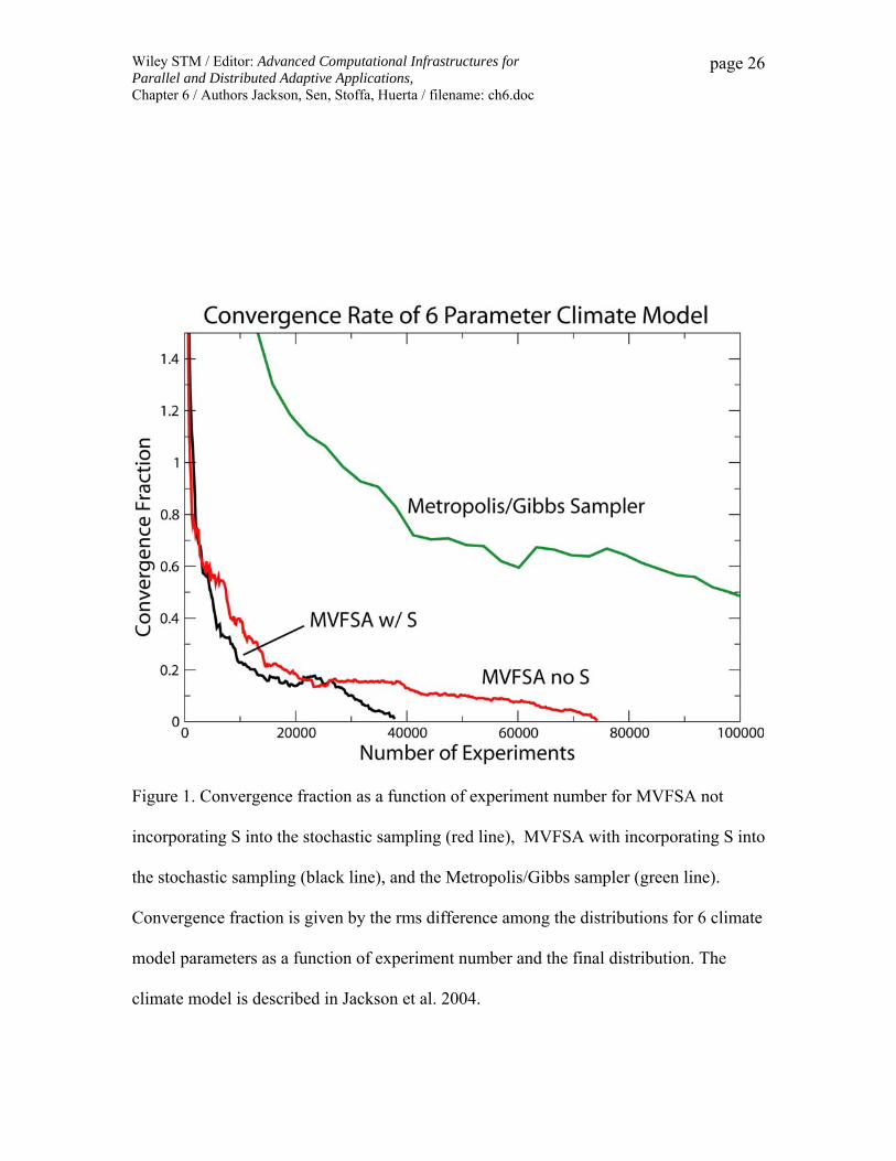
chains. Because of its data-directed sampling, MVFSA can be several orders of

magnitude more efficient than the Metropolis/Gibbs sampler (Figure 1). So the

combination of the sampling efficiency and the fact that one can separate the problem

into multiple pieces brings a new class of problems within reach of Bayesian stochastic

inversion.

4. Application to Climate Prediction Within the Bayesian formulation of probability, the likelihood of a given choice in

parameters is measured by an exponential of the effects of those parameters on model

performance (i.e. the cost function) relative to all other parameter choices tested. The use

of exponential implies Gaussian errors in both the data and observations. Many potential

applications of Bayesian stochastic inversion may not know or may not depend heavily

on quantifying these errors. For instance, in some cases it may be sufficient to simply

identify the locations of the peaks in the PPD and exhibit the uncertainty as a qualitative


page 11

re-weighting of the PPD given slightly different scaling factors, S, for the uncertainty in

size in the error normalization (data covariance) part of the metric of model performance,

∫ ⋅−

⋅−=mm

mmdES

ESPPD))(exp(

))(exp()( . (3)

For the climate prediction problem, where there is more interest in quantifying the

likelihood of extremes, it is necessary to develop a more formal way to incorporate

information about sources of uncertainty. In the following two sections, we discuss why

there exists a need for incorporating prior information acknowledging uncertainties in

selecting ‘S’ into the definition of the metric of model performance and its role in

improving the efficiency and accuracy of estimating the PPD.

4.1 Definition of the Metric of Model

Performance

The cost function E(m) contains an inverse of the data covariance matrix which

provides a means to normalize the significance of model-data mismatch among N

different fields dobs (e.g. surface air temperature, precipitation, etc…) and model

predictions g(m) at M points (note that each field may contain a different number of

points M),

1−C

[∑=

− −−=N

iiobs

Tobs gg

NE

1

1 ))(())((21)( mdCmdm ] . (4)

Equation (1) includes vector m of model parameter values and T for the matrix transpose.

The data covariance matrix includes information about sources of observational or model


page 12

uncertainty, including information about uncertainty originating from natural (internal)

variability, measurement errors, or theory. This form of the mean square error E is the

appropriate form for assessing more rigorously the statistical significance of modeled-

observational differences when it is known that distributions of model and observational

uncertainty are Gaussian. Our focus here will be entirely on sources of uncertainty that

arise from natural variability.

If one assumes uncertainties are spatially uncorrelated, the data covariance matrix will

contain non-zero elements only along the diagonal. When considering uncertainty

originating from spatially uncorrelated natural variability, each of these elements is equal

to the variance of the natural variability within the corresponding grid point where model

predictions are compared to observations. However data points are correlated in space,

season, and among fields. Some points and/or fields have very little associated variance,

such as rain over a desert. The cost function can be very sensitive to the choices one

makes in accounting for these correlations and/or singularities within the data covariance

matrix (Mu et al., 2004). Estimating normalizing factors for complex systems is an area

of active research (Gelman et al., 2004, see page 345). Although not satisfactory to a

statistician, some have treated this unknown through a re-weighting of the posterior

distribution (i.e. S within equation 3). The problem is that such a re-weighting does not

give the statistical sampling algorithm the opportunity to only sample from the posterior

which can lead to in-efficiencies and biases in the results. A more statistically correct

procedure would be to introduce a renormalizing factor before sampling. One empirical

Bayesian approach is to estimate S in advanced through an ensemble of experiment in


page 13

which one imposes uncertainties. For instance, in the climate problem where the

uncertainty is from natural variability, one may consider how the cost function would be

affected if the climate model (or data) were taken from different segments of a long

integration. One may estimate a fixed re-normalizing factor to be ES ∆= 2 where

represents the 2σ range in cost function values that arise from internal

variability. One may then apply the logic that parameter sets that are ∆E away from the

optimal parameter set will be given a likelihood measure of exp(-2), which is equivalent

to the 95% probability measure for a normalized Gaussian distribution.

095 EEE −=∆

4.2 Incorporating Uncertainties in Error

Normalization in the Prior

The re-weighting of samples according to equation (3) give a skewed perspective of the

PPD as it tends to have more narrow peaks and fat tails relative to a cost function that had

been correctly normalized. This is because correlations among constraints in the data tend

to increase the significance of changes in the cost function. Thus stochastic sampling

uninformed about the effects of these correlations will tend to sample more frequently the

regions that end up being weighted down in equation (3). This represents a sampling

inefficiency.

Along the lines suggested by Gelman et al. (2004) it is possible to treat S as one of the

uncertain parameters within MVFSA and use principles of Bayesian inference to select


page 14

candidate choices of S from a prior Gamma distribution whose mean and variance is

determined by a process similar to the choice of S in Section 4.1. The choice of a Gamma

distribution was mostly for mathematical convenience and given that a Gamma prior is

"conditionally conjugate" to our definition of the cost function. It is a mathematical way

to express uncertainties in the denominator (i.e. the variance). The Gamma distribution

looks alike a skewed Gaussian distribution with no probability for a value of 0, a mean

value that corresponds to the choice of S from the previous section, and a tail that

conveys uncertainties in defining an appropriate S. In a fully Bayesian approach, one can

construct candidate choices of S to depend on a corresponding evaluation of E(m) in

order to incorporate uncertainties in the data covariance matrix into the stochastic

sampling algorithm (Jackson et al, in prep).

Although this revised method adds a randomly generated number S to the

acceptance/rejection criterion (equation 1), there can be significant improvements in the

accuracy and efficiency (Figure 1) to estimating the PPD. In fact, samples selected in the

case where S is included through a prior no longer require weighting for estimating the

PPD as these samples are now assumed to be drawn directly from a distribution that is

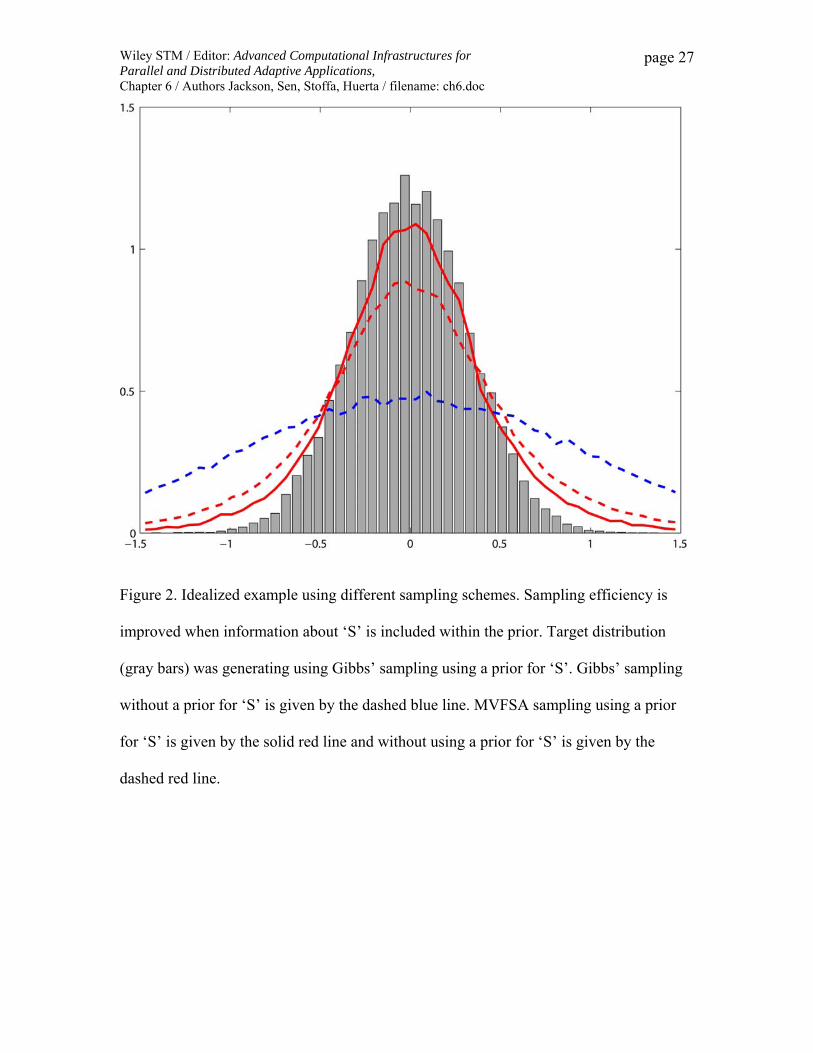
proportional to the actual PPD. The effect of this choice can be dramatic as illustrated in

Figure 2 where the PPD derived from including S as a prior is a much better match to the

target distribution of an idealized example than without it.

5. Results


page 15

The MVFSA stochastic sampler has been applied to estimating the PPD of six

parameters (Table 2) of the Community Atmosphere Model version 3.1 (CAM3.1)

important to clouds and convection as constrained by observations or reanalysis of 15

fields separated into 4 seasons and 6 regions covering the globe (Mu et al., 2004). In

addition MVFSA incorporates a prior distribution estimate for S, the parameter

controlling inadequacies of properly defining the data covariance matrix (Jackson et al, in

prep).

Each experiment testing the sensitivity of CAM3.1 to combined changes in select

parameters follows an experimental design in which the model is forced by observed sea

surface temperatures (SST) and sea ice for an 11-year period (March 1990 through Feb.

2001). The model includes 26 vertical levels and uses an approximately 2.8˚ latitude by

2.8˚ longitude (T42) resolution.

Up to this point 518 experiments have been completed over 6 independent VFSA

convergence attempt “lines”. Each line starts at a randomly chosen point in the multi-

dimensional parameter space. Each model experiment runs in parallel over 64 processors,

bringing the total number of processors being occupied at any point in time to 384. The

average number of experiments that we anticipate will be required to reach convergence

for each line is 150 (Jackson et al, 2004). We therefore estimate that we are about two

thirds of the way toward a stationary estimate of the PPD.


page 16

Of the 518 completed experiments, 332 configurations have cost values the same or

better relative to the default model configuration with the optimal experiments in each

line averaging a respectable 10% improvement in their cost values. The size of the cost

function gives a normalized perspective of the distance between observations and model

predictions with the units relating to the size of the effect of internal variability on each

component. Large cost values tend to be associated with fields that have very little

variability. In this case the field with the largest associated cost value in the default model

configuration is the annual mean global mean radiative balance at the top of the

atmosphere with a value of 202 cost units. The field with the lowest cost value is

precipitation with a value of 24.2 cost units.

We have separately analyzed the six top performing experiments, one for each of the

independent lines considered. The fields that improved the most across these six

experiments were shortwave radiation reaching the surface (averaging 14%

improvement), net radiative balance at the top of the atmosphere (33% improvement),

and precipitation (12% improvement). However, the performance gains or losses for the

other fields were not consistent. The similar cost values achieved for all six optimal

model configurations is achieved through different compromises in model skill for

predicting particular fields.

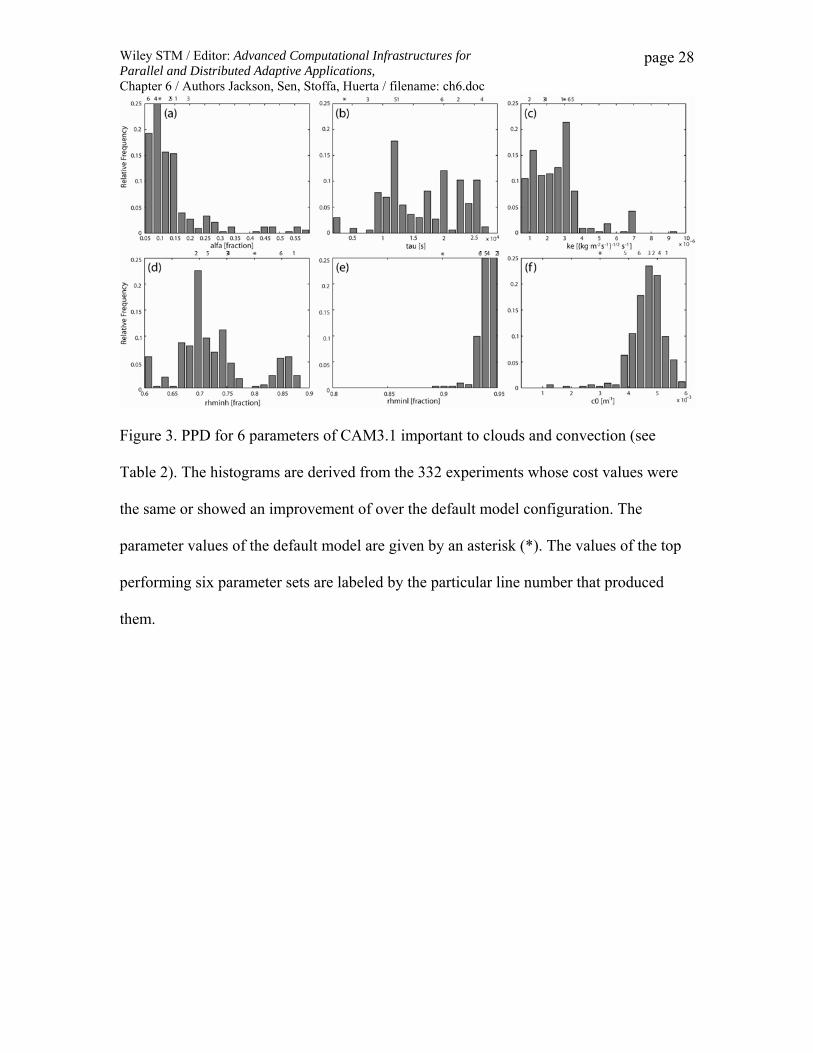
The marginal PPD for each of the six model parameters along with the position of the

default model and the optimal values chosen by the six lines is shown in Figure 3. The

PPD is generated only from the 332 configurations that have the same or better cost than


page 17

the default configuration. The range of parameter values that improved model

performance is quite broad for all parameters except for the critical relative humidity for

low cloud formation. Also of interest is the desired result that the six optimal parameter

sets are representative of the uncertainty as quantified by the PPD. Capturing climate

model parametric uncertainties within a limited number of candidate model

configurations is the key step in quantifying observational constraints on these important

degrees of freedom for model development. For instance, one may use these different

parameter sets to test the impacts of these uncertainties on the model’s sensitivity to CO2

forcing. Although we are still a third of the away from completing the number of

necessary experiments to draw a firm conclusion, the implication of the wide ranges

apparent in Figure 3 is that it may be very difficult to use available observations to

constrain sufficiently some of the choices that need to be made in assigning values to

parameters that are involved in clouds and convection which are processes thought to be

key sources of climate prediction uncertainty.

6. Summary

The increase in availability in distributed computing provides an opportunity for

the climate sciences to address more quantitatively the sources and impacts of

uncertainties in climate model development on climate predictions. This is achieved

through a selection of alternate climate model configurations that reflect the scientific

values for how these models are constrained by observations (i.e. the definition of the

cost function). One of the barriers to achieving this goal is the substantial computational


page 18

expense of climate models where the ideal choice of multiple parameter values is inter-

dependent. For these cases, one needs to draw inferences about the relative likelihood of

different possible choices from a random sampling of candidate parameter combinations

that do not bias the end result. Data directed importance sampling achieves improved

efficiency from sampling more often, and in proportion to the final PPD, those regions of

parameter space that contribute effectively to the PPD. There exist many types of

stochastic samplers that make use of data-direction. However, many of these approaches

depend on the sequential integration of experiments which make it difficult to fully

exploit available computational resources. Moreover, the efficiency of most methods

depends on knowledge about the characteristics of the problem which may be difficult to

gage without significant experimentation. We present Multiple Very Fast Simulated

Annealing (MVFSA) as an alternative which is less sensitive to problem characteristics

and produces helpful estimates of the PPD.

We also show that additional improvements in accuracy and efficiency of the

MVFSA algorithm can be incorporated into data-directed importance samplers when

prior information is incorporated about the size of the effects of sources of uncertainty on

the cost function through a parameter ‘S’ which is conceptually correcting for errors in

defining a data covariance matrix that appropriately accounts for correlations that may

exist among the many data constraints.

The results of estimating a PPD for 6 parameters of the CAM3.1 climate model

reinforce the notion that there exist many possible model configurations that can do an


page 19

equally adequate job in reproducing a multi-field average skill score. More sampling will

be required to establish with greater confidence the relative likelihood of the solutions

that have been identified so far. The main point of this exercise is to illustrate the

practicality of data-directed importance sampling and uncertainty characterization of

parameters within a non-idealized climate model.

References

Allen, M., 1999: Do-it-yourself climate prediction. Nature, 401, 642.

Annan, J. D., and J. C. Hargreaves (2007), Efficient estimation and ensemble generation

in climate modeling, Phil. Trans. R. Soc. A, 365, 2077-2088, doi:10.1098/rsta.2007.2067.

Barhen, J., J.G. Berryman, L. Borcea, J. Dennis, C. de Groot-Hedlin, F. Gilbert, P. Gill,

M. Heinkenschloss, L. Johnson, T. McEvilly, J. More, G. Newman, D. Oldenburg, P.

Parker, B. Porto, M. Sen, V. Torczon, D. Vasco, and N.B.Woodward, 2000: Optimization

and Geophysical Inverse Problems, Report of a Workshop at San Jose, California,

February 5-6, 1999. Lawrence Berkeley National Laboratory report number 46959, 33pp.

Bowman, K. P., J Sacks, and Y-F. Chang, 1993: On the design and analysis of numerical

experiments, J. Atmos. Sci., 50, 1267-1278.


page 20

Chapman, W. L., W. J. Welch, K. P. Bowman, J. Sacks, and J. E. Walsh, 1994: Arctic sea

ice variability: Model sensitivities and a multidecadal simulation, J. Geophys. Res.,

99(C1), 919-935.

Cubasch, U., G.A. Meehl, G.J. Boer, R.J. Stouffer, M. Dix, A. Noda, C.A. Senior, S.

Raper, K.S. Yap, 2001: Projections of Future Climate Change. Climate Change 2001:

The Scientific Basis. Contribution of Working Group I to the Third Assessment Report of

the Intergovernmental Panel on Climate Change, Houghton, J.T., Y. Ding, D.J. Griggs,

M. Noguer, P.J. van der Linden, X. Dai, K. Maskell, and C.A. Johnson, Eds., Cambridge

University Press, Cambridge, United Kingdom and New York, NY, USA, 881pp.

Evensen, G. 2003. The ensemble Kalman filter: Theoretical formulation and practical

implementation. Ocean Dyn. 53, 343–367.

Forest, C., M. R. Allen, P. H. Stone, and A. P. Sokolov, 2000: Constraining uncertainties

in climate models using climate change detection techniques. Geophys. Res. Lett., 27(4),

569-572.


page 21

Forest, C., M. R. Allen, A. P. Sokolov, and P. H. Stone, 2001: Constraining climate

model properties using optimal fingerprint detection methods. Climate Dynamics, 18,

277-295.

Forest, C., P. H. Stone, A. P. Sokolov, M. R. Allen, and M. D. Webster, 2002:

Quantifying uncertainties in climate system properties with the use of recent climate

observations. Science, 295, 113-117.

Gates, W. L., J. S. Boyle, C. Covey, C. G. Dease, C. M. Doutriaux, R. S. Drach, M.

Fiorino, P. J Gleckler, J. J. Hnilo, S. M. Marlais, T. J. Phillips, G. L. Potter, B. D. Santer,

K. R. Sperber, K. E. Taylor, D. N. Williams, 1999: An Overview of the Results of the

Atmospheric Model Intercomparison Project (AMIP I). Bulletin of the American

Meteorological Society 80(1), 29-56.

Gelman, A., J. B. Carlin, H. S. Stern, and D. B. Rubin (2004) Bayesian Data Analysis,

Second Ed., Chapman & Hall/CRC, 668p.

Grell, G. A., and D. Dévényi (2002), A generalized approach to parameterizing

convection combining ensemble and data assimilation techniques, Geophys. Res. Lett.,

29(14), 1693, doi:10.1029/2002GL015311


page 22

Jackson, C., M. Sen, and P. Stoffa (2004) An Efficient Stochastic Bayesian Approach to

Optimal Parameter and Uncertainty Estimation for Climate Model Predictions, Journal of

Climate, 17(14), 2828-2841.

Joussaume, S., and K.E. Taylor, 2000: The Paleoclimate Modeling Intercomparison

Project. Paleoclimate Modeling Intercomparison Project (PMIP): proceedings of the

third PMIP workshop, Canada, 4-8 October 1999, P. Braconnot, Ed., WCRP-111,

WMO/TD-1007, pp. 271.

Kheshgi, H., B.S. White, 2001: Testing distributed parameter hypotheses for the

detection of climate change. Journal of Climate, 14, 3464-3481.

Lea, D.J., M.R. Allen and T.W.N. Haine, 2000: Sensitivity analysis of the climate of a

chaotic system. Tellus, 52A, 523-532.

LeTreut, H., and B.J. McAvaney, 2000: A model intercomparison of equilibrium climate

change in response to CO2 doubling. Note du Pole de Modelisation de l'IPSL, Number

18, Institut Pierre Simon LaPlace, Paris, France.


page 23

McAvaney, B.J., C. Covey, S. Joussaume, V. Kattsov, A. Kitoh, W Ogana, A.J. Pitman,

A.J. Weaver, R.A. Wood, and Z.-C. Zhao, 2001: Model Evaluation. Climate Change

2001: The Scientific Basis. Contribution of Working Group I to the Third Assessment

Report of the Intergovernmental Panel on Climate Change, Houghton, J.T., Y. Ding, D.J.

Griggs, M. Noguer, P.J. van der Linden, X. Dai, K. Maskell, and C.A. Johnson, Eds.,

Cambridge University Press, Cambridge, United Kingdom and New York, NY, USA,

881pp.

Meehl, G.A., G.J. Boer, C. Covey, M. Latif, R.J. Stouffer, 2000: The Coupled Model

Intercomparison Project (CMIP). Bulletin of the American Meteorological Society 81(2),

313-318.

Mu, Q., C. S. Jackson, and P. L. Stoffa (2004) A multivariate empirical-orthogonal-

function-based measure of climate model performance, J. Geophys. Res., 109, D15101,

doi:10.1029/2004JD004584.

Sacks, J., S. B. Schiller, and W. J. Welch, 1989: Designs for computer experiments,

Technometrics, 31, 41-47.


page 24

Santner, T. J., B. J. Williams, and W. I. Notz (2003) The Design and Analysis of

Computer Experiments, Springer-Verlag, Inc.

Sen, M. K., and P. L. Stoffa (1996) Bayesian inference, Gibbs’ sampler and uncertainty

estimation in geophysical inversion. Geophys. Prospect., 44, 313–350.

Stainforth, D. A., T. Aina, C. Christensen, M. Collins, N. Faull, D. J. Frame, J. A.

Kettleborough, S. Knight, A. Martin, J. M. Murphy, C. Piani, D. Sexton, L. A. Smith, R.

A. Spicer, A. J. Thorpe and M. R. Allen, 2005: Uncertainty in predictions of the climate

response to rising levels of greenhouse gases Nature 433, 403-406.

Welch, W. J., R. J. Buck, J. Sacks, H. P. Wynn, T. J. Mitchell, and M D. Morris, 1992:

Screening, predicting, and computer experiments, Technometrics, 34, 15-25.

Williams K. D., C. A. Senior, J. F. B. Mitchell, 2001: Transient climate change in the

Hadley Centre models: The role of physical processes, Journal of Climate, 14 (12), 2659-

2674.


page 25

Table 1. Performance of CAM3.1 over a cluster of Dell PowerEdge 1955 Blade servers

# of processors

1 2 4 8 16 32 6

Simulated years/wall clock day

0.92 1.70 2.91 5.56 10.26 17.91 2

Simulated years/wall clock day

per processor

.92 .883 .729 .696 .641 .560 .4

Table 2. Names and descriptions of parameters important to clouds and convection

in CAM3.1

Parameter description

RHMINL critical relative humidity for low cloud formation

RHMINH critical relative humidity for high cloud formation

ALFA initial cloud downdraft mass flux

TAU rate at which convective clouds consume available potential energy

ke environmental air to cloud entrainment rate coefficient

c0 deep convection precipitation production efficiency parameter


page 26

Figure 1. Convergence fraction as a function of experiment number for MVFSA not

incorporating S into the stochastic sampling (red line), MVFSA with incorporating S into

the stochastic sampling (black line), and the Metropolis/Gibbs sampler (green line).

Convergence fraction is given by the rms difference among the distributions for 6 climate

model parameters as a function of experiment number and the final distribution. The

climate model is described in Jackson et al. 2004.


page 27

Figure 2. Idealized example using different sampling schemes. Sampling efficiency is

improved when information about ‘S’ is included within the prior. Target distribution

(gray bars) was generating using Gibbs’ sampling using a prior for ‘S’. Gibbs’ sampling

without a prior for ‘S’ is given by the dashed blue line. MVFSA sampling using a prior

for ‘S’ is given by the solid red line and without using a prior for ‘S’ is given by the

dashed red line.


page 28

Figure 3. PPD for 6 parameters of CAM3.1 important to clouds and convection (see

Table 2). The histograms are derived from the 332 experiments whose cost values were

the same or showed an improvement of over the default model configuration. The

parameter values of the default model are given by an asterisk (*). The values of the top

performing six parameter sets are labeled by the particular line number that produced

them.

Documents

Chapter 6 Data Directed Importance Sampling for …ghuerta/papers/manuscript_v2_combined.pdf · Wiley STM / Editor: Advanced Computational Infrastructures for Parallel and Distributed