Embed Size (px)
Citation preview

Chapter 6Double-SidebandSuppressed-CarrierAmplitude Modulation
Contents
Slide 1 Double-Sideband Suppressed-CarrierAmplitude Modulation
Slide 2 Spectrum of a DSBSC-AM SignalSlide 3 Why Called Double-SidebandSlide 4 Ideal Coherent ReceiverSlide 5 Coherent Receiver AnalysisSlide 6 Spectra in DSBSC-AM SystemSlide 7 Demodulator Using the Pre-EnvelopeSlide 8 Costas Loop DemodulatorSlide 9 Costas Loop (cont. 1)Slide 10 Costas Loop (cont. 2)Slide 11 Costas Loop (cont. 3)Slide 12 Costas Loop (cont. 4)
Generating the Phase EstimateSlide 13 Costas Loop (cont. 4)
Generating the Phase Estimate (cont.)Slide 14 Linearized Loop ModelSlide 15 Linearized Loop Model (cont.)

Slide 15 Performance with Additive NoiseSlide 16 Performance with Noise (cont. 1)
Slide 17 Laboratory Exercises andExperiments for the Costas Loop
Slide 18 Theoretical Design ExercisesSlide 19 Hardware ExperimentsSlide 20 Hardware Experiments (cont. 1)Slide 21 Hardware Experiments (cont. 2)Slide 22 Hardware Experiments (cont. 3)
6-ii

✬
✫
✩
✪
Chapter 6
Double-Sideband Suppressed-Carrier
Amplitude Modulation and
Coherent Detection
Standard AM contains a sinusoidal component at
the carrier frequency which does not convey any
message information. It is included to create a
positive envelope which allows demodulation by
a simple inexpensive envelope detector. From an
information theory point of view, the power in the
carrier component is wasted.
Definition of the DSBSC-AM Signal
Let m(t) be a bandlimited baseband message
signal with cutoff frequency W . The DSBSC-AM
signal corresponding to m(t) is
s(t) = Acm(t) cosωct
This is the same as AM except with the sinusoidal
carrier component eliminated.
6-1

✬
✫
✩
✪
A message m(t) typically has positive and negative
values so it can not be recovered from s(t) by an
envelope detector. A demodulation method called
coherent demodulation will be explored in this
experiment.
Spectrum of a DSBSC-AM Signal
The Fourier transform of s(t) is
S(ω) = 0.5AcM(ω − ωc) + 0.5AcM(ω + ωc)
This is the same as the AM spectrum but with the
discrete line at the carrier frequency removed. An
example is shown in the figure on Slide 6-6.
• The carrier frequency must satisfy the bound,
ωc > W so that the two shifted baseband
transforms do not overlap.
• When they overlap foldover is said to have
occurred and perfect demodulation cannot be
achieved.
6-2

✬
✫
✩
✪
Why the Term Double-Sideband is
Used
When m(t) is a real signal, M(−ω) = M(ω) and
S(ωc − ω) = S(ωc + ω) for 0 ≤ ω ≤ ωc
• This equation shows that the component at
frequency ωc + ω contains exactly the same
information as the component at ωc − ω since
one can be uniquely determined from the
other by taking the complex conjugate.
• The portion of the spectrum for |ω| > ωc is
called the upper sideband and the portion for
|ω| < ωc is called the lower sideband.
• The fact that the modulated signal contains
both portions of the spectrum explains why
the term, double-sideband, is used.
6-3

✬
✫
✩
✪
The Ideal Coherent Receiver for
DSBSC-AM
��
��
- - - -
?
Local
Oscillator
�
s(t) m
1
(t)s
1
(t)
2 cos!
c
t
Bandpass
Receive Filter
Lowpass
Post Detection Filter
Mixer
B(!) G(!)
First, the received signal is passed through
a bandpass filter B(ω) centered at the carrier
frequency that passes the DSBSC signal and
eliminates out-of-band noise.
The output of B(ω) is then multiplied by
a replica of the carrier wave. This replica is
generated by a device called the local oscillator
(LO) in the receiver. The device that performs
the product is often called a product modulator or
balanced mixer.
6-4

✬
✫
✩
✪
Ideal Coherent Receiver Analysis
Assuming no noise, the product is
s1(t) = 2s(t) cosωct = 2Acm(t) cos2 ωct
= Acm(t) +Acm(t) cos 2ωct
The Fourier transform of the product modulator
output is
S1(ω) = AcM(ω) + 0.5AcM(ω + 2ωc)
+ 0.5AcM(ω − 2ωc)
and is illustrated in the figure on Slide 6-6. The
first term on the right-hand side is proportional to
the desired message. The second term has spectral
components centered around −2ωc and 2ωc. The
corresponding terms can be seen in S1(ω). The
undesired high frequency terms are eliminated by
the final lowpass filter which has cutoff frequency
W . This is often called a post detection filter.
6-5

✬
✫
✩
✪
Spectra in DSBSC-AM
Communication System
H
H
H
H�
�
�
�
H
H
H
H�
�
�
��
�
�
�H
H
H
H
H
H
H
H�
�
�
�H
H
H
H�
�
�
�
@
@
@
@�
�
�
� �
�
�
�
�
�
��
�
�
�
��
A
AU
J
J
J
M(!)
!
!
0
0
S(!)
S
1
(!)
!
0 W�W
!
c
�!
c
2!
c
�2!
c
0:5A
c
M(! � !
c
)
0:5A
c
M(! + !
c
)
0:5A
c
M(! � 2!
c
)
A
c
M(!)
0:5A
c
M(! + 2!
c
)
(a) Fourier Transform of Baseband Message
(b) Fourier Transform of DSBSC-AM Signal
(c) Fourier Transform of Mixer Output
6-6

✬
✫
✩
✪
A Demodulator Using the
Pre-Envelope
An alternative method of demodulation is to first
form the pre-envelope of the received signal. With
no additive noise, this is
s+(t) = s(t) + js(t)
= Acm(t) cosωct+ jAcm(t) sinωct
= Acm(t)ejωct
The baseband message is then recovered to within
a scale factor by forming the complex product
s+(t)e−jωct = Acm(t)
6-7

✬
✫
✩
✪
The Costas Loop Demodulator
The Costas loop locks to the carrier frequency
and phase and performs nearly ideal coherent
demodulation.
G(ω) ✲
✒✑✓✏
✲
✛✛✛❄
✛
✻
✻
✛
❄
✻
✲✲
✲
❄
✻
✻
×
e−j(·)
z−1 α
β
1− z−1
e−jφ(nT ) = e−j(ωcnT+θ2)
ωcT
σ(nT )
−j signω
φ(nT )
q(nT )
m1(nT )
s(nT )
m2(nT )
s(nT )
c1(nT ) = ℜe{s+(nT )e−j(ωcnT+θ2)}
+ +
×✒✑✓✏
c2(nT ) = ℑm{s+(nT )e−j(ωcnT+θ2)}
✒✑✓✏
✒✑✓✏
Second-Order Costas Loop Demodulator
Let the received signal after it has passed through
a bandpass receive filter be
s(nT ) = Acm(nT ) cos(ωcnT + θ1)
where ωc is the nominal carrier frequency and θ1
is a constant or slowly changing phase angle.
6-8

✬
✫
✩
✪
Costas Loop (cont. 1)
• The first step is to form the complex envelope
s+(nT ) = s(nT ) + js(nT ) = Acm(nT )ej(ωcnT+θ1)
The parallel solid and dotted lines in the figure
represent complex signals with the solid line
corresponding to the real part and dotted line to
the imaginary part.
• The system generates an estimate φ(nT ) of the
angle of the received signal that can expressed as
φ(nT ) = ωcnT + θ2(nT )
It is passed through the complex exponential box
to give the local oscillator signal e−jφ(nT ). The
method for generating this angle will be explained
shortly.
6-9
✬
✫
✩
✪
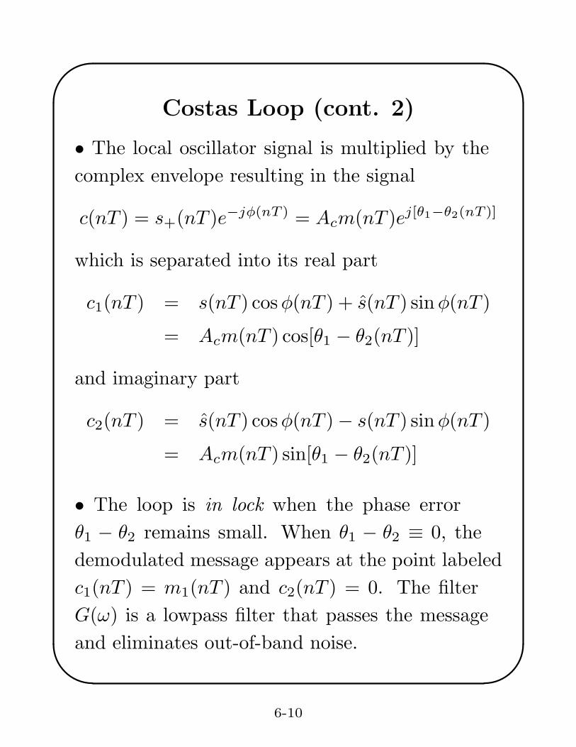
Costas Loop (cont. 2)
• The local oscillator signal is multiplied by the
complex envelope resulting in the signal
c(nT ) = s+(nT )e−jφ(nT ) = Acm(nT )ej[θ1−θ2(nT )]
which is separated into its real part
c1(nT ) = s(nT ) cosφ(nT ) + s(nT ) sinφ(nT )
= Acm(nT ) cos[θ1 − θ2(nT )]
and imaginary part
c2(nT ) = s(nT ) cosφ(nT )− s(nT ) sinφ(nT )
= Acm(nT ) sin[θ1 − θ2(nT )]
• The loop is in lock when the phase error
θ1 − θ2 remains small. When θ1 − θ2 ≡ 0, the
demodulated message appears at the point labeled
c1(nT ) = m1(nT ) and c2(nT ) = 0. The filter
G(ω) is a lowpass filter that passes the message
and eliminates out-of-band noise.
6-10

✬
✫
✩
✪
Costas Loop (cont. 3)
A lock detection strategy is to lowpass filter
c22(nT ) and declare that the loop is in lock when
this signal falls below a threshold.
• The real and imaginary parts are multiplied,
resulting in the signal
q(nT ) = c1(nT )c2(nT )
= A2cm
2(nT ) cos[θ1 − θ2(nT )] sin[θ1
− θ2(nT )]
= 0.5A2cm
2(nT ) sin{2[θ1 − θ2(nT )]}
Notice that when θ1 and θ2 differ by less than
90 degrees, q(nT ) has the same sign as the phase
error θ1 − θ2, so it indicates in which direction
the local phase estimate θ2 should be changed to
reduce the phase error to zero. When the loop is
in lock, the small angle approximation sinx ≃ x
can be used to accurately approximate q(nT ) by
q(nT ) ≃ A2cm
2(nT )[θ1 − θ2(nT )]
for |θ1 − θ2(nT )| ≪ 1
6-11

✬
✫
✩
✪
Costas Loop (cont. 4)
Generating the Phase Estimate
The lower half of the block diagram generates the
loop’s estimate of the phase of the received signal
by computing
φ((n+ 1)T ) = φ(nT ) + ωcT + αq(nT ) + σ(nT )
where
σ(nT ) = βq(nT ) + σ((n− 1)T )
and α and β are small positive constants with
β < α/50, typically.
• The basic philosophy behind these equations
is that at each new sampling instant the loop’s
phase estimate is incremented by the nominal
change in carrier phase between samples ωcT
plus a small correction term αq(nT ) roughly
proportional to the phase error.
6-12

✬
✫
✩
✪
Generating the Phase Estimate
(cont.)
• Notice that when q(nT ) = 0 for all n, φ(nT )
is the linear ramp
φ(nT ) = ωcnT + φ(0)
which has a slope equal to the nominal carrier
frequency.
• The accumulator block β/(1−z−1) is included
to allow the loop to track a carrier input
phase θ1(nT ) that is a linear ramp with zero
steady-state error. The input phase has this
form when there is a frequency offset between
the received and local carrier frequencies.
The output σ(nT ) of the accumulator reaches
the steady-state value ∆ω T which is the
phase change between samples caused by the
frequency offset ∆ω.
6-13

✬
✫
✩
✪
Linearized Loop Model
The Costas loop is a nonlinear and time-varying
system. However, when it is in lock, it can be ac-
curately approximated by a linear, time-invariant
system by using the small angle approximations
and replacing m2(nT ) by its expected value. Let
k1 = A2c E{m2(nT )}
and further approximate q(nT ) by
q(nT ) ≃ k1[θ1 − θ2(nT )]
��
��
�
��
?
+
k
1
�
1� z
�1
�
��
��
+
��
��
+
-
6
��
?
-
�
1
(nT )
�
2
(nT )
�
z
�1
Linearized Loop Block Diagram
6-14

✬
✫
✩
✪
Linearized Loop Model (cont.)
The transfer function for the linearized loop is
H(z) =Θ2(z)
Θ1(z)
=k1(α+ β)
(
1− αα+β
z−1)
z−1
1− [2− k1(α+ β)]z−1 + (1− k1α)z−2
The frequency response is obtained by letting
z = ejωT and has the shape of a narrowband
lowpass filter for small α and β. The closed loop
gain at zero frequency is H(1) = 1.
Performance with Additive Noise
Suppose the received signal without noise is
s(t) = a(t) cos(ωct)
and corrupting band limited additive noise is
n(t) = nI(t) cos(ωct)− nQ(t) sin(ωct)
where nI(t) and nQ(t) are the independent lowpass
inphase and quadrature noise components.
6-15

✬
✫
✩
✪
Performance with Additive Noise
(cont. 1)
Then, the received signal is
r(t) = s(t) + n(t)
= [a(t) + nI(t)] cos(ωct)− nQ(t) sin(ωct)
The Hilbert transform of the received signal is
r(t) = [a(t) + nI(t)] sin(ωct) + nQ(t) cos(ωct)
and the pre-envelope is
r+(t) = r(t) + jr(t)
= [a(t) + nI(t)][cos(ωct) + j sin(ωct)]
+jnQ(t)[cos(ωct) + j sin(ωct)]
= [a(t) + nI(t) + jnQ(t)]ejωct
The demodulator output is
c1(t) = Re{
r+(t)e−jωct
}
= a(t) + nI(t)
Notice that only the inphase noise component is
present in the output. The square-law demodula-
tor output contains both nI(t) and nQ(t).
6-16

✬
✫
✩
✪
Laboratory Exercises and
Experiments for the Costas
Loop
Use the signal generator to generate the AM wave
s(t) = Acm(t) cos 2πfct
where
Ac = 1
m(t) = 1 + 0.4 cos(2πfmt+Φ)
fc = 4000 Hz
fm = 400 Hz
where Φ is a random variable uniform over [0, 2π).
Actually, s(t) is an AM signal with modulation
index µ = 0.4. However, it can also be considered
to be a DSBSC-AM signal with m(t) containing
a dc value and all the theory for the Costas loop
still holds.
6-17

✬
✫
✩
✪
Theoretical Design Exercises
In these exercises you will do theoretical compu-
tations to select the Costas loop parameters for a
reasonable design. Do the following:
1. Compute k1 by the equation on Slide 6-14.
2. Choose some small values for the loop filter
constants, for example, α = 0.01 and β =
0.0002. You will find that β should be small
relative to α, perhaps, less than α/50, to get
a transient response without excess ripple.
Recursively compute the response of the
linearized loop to a unit step in θ1(nT ) using
the following realization of H(z):
θ2(nT ) = k1[(α+β)θ1((n− 1)T )−αθ1((n−2)T )]
+ [2− k1(α+ β)]θ2((n− 1)T )
− (1− k1α)θ2((n− 2)T )
Continue the computations until θ2(nT ) gets close
to its final value and plot the result. Repeat this
step for different values of α and β until you find
a pair for which the step response settles to its
final value in about 0.5 seconds.
6-18

✬
✫
✩
✪
3. Compute and plot the closed loop amplitude
response A(f) = 20 log10
|H(ej2πf/fs)| for the
values of α and β finally selected in the previous
step.
Hardware Experiments
Write a C/assembly language program for the
TMS320C6713 to do the following:
1. Initialize the DSP and codec as in Chapter 2.
2. Read samples from the ADC at a 16 kHz
sampling rate.
3. Demodulate the input signal with a Costas
loop. Make sure to keep the LO angle confined
to 0 ≤ φ(nT ) ≤ 2π.
4. Send the demodulated signal samples to the
DAC at a 16 kHz rate.
6-19

✬
✫
✩
✪
Hardware Experiments (cont. 1)
Perform the following exercises:
1. Connect the signal generator to the DSK line
input and set it to generate the AM signal
s(t) defined above. Connect the DSK line
output to the oscilloscope and debug your
DSP program if the output is not m(t).
2. Investigate your Costas loop performance in
the presence of a frequency offset.
• First set the signal generator carrier fre-
quency to the nominal 4 kHz value and let
your loop achieve lock.
• Then slowly change the carrier frequency to
a slightly different value and see if the loop
remains locked.
• Use Code Composer to watch σ(nT ) in your
DSP program and check that it has the correct
steady-state value for the frequency offset you
are using.
6-20

✬
✫
✩
✪
Hardware Experiments (cont. 2)
Creating a Watch Window
To watch a variable, right click on the
variable and then left click on “Add Watch
Expression...” Enter the variable name in the
box of the “Add Watch Expression” window.
You can move and resize the watch window as
you prefer.
3. The linearized equations describe the loop
behavior accurately when it is in lock. When
there is a large initial frequency offset, the
behavior is quite different.
• Experimentally investigate this behavior by
setting the signal generator carrier frequency
to a value that differs by 30 Hz or more
from the nominal 4 kHz value and starting
the Costas loop. The loop may take a much
longer time than you expected to achieve lock
and may not even lock. This is called its pull
in behavior.
6-21
✬
✫
✩
✪
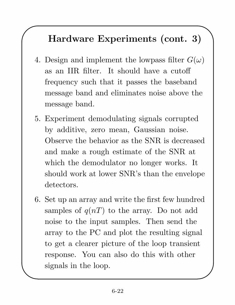
Hardware Experiments (cont. 3)
4. Design and implement the lowpass filter G(ω)
as an IIR filter. It should have a cutoff
frequency such that it passes the baseband
message band and eliminates noise above the
message band.
5. Experiment demodulating signals corrupted
by additive, zero mean, Gaussian noise.
Observe the behavior as the SNR is decreased
and make a rough estimate of the SNR at
which the demodulator no longer works. It
should work at lower SNR’s than the envelope
detectors.
6. Set up an array and write the first few hundred
samples of q(nT ) to the array. Do not add
noise to the input samples. Then send the
array to the PC and plot the resulting signal
to get a clearer picture of the loop transient
response. You can also do this with other
signals in the loop.
6-22