Chapter-6 Regional Variation and Convergence in …shodhganga.inflibnet.ac.in/bitstream/10603/68496/13/13_chapter 6.pdf · It is well known that there exist wide regional variations

Regional Variation and Convergence in Agricultural Development in India

Chapter-6


6.1 Introduction

Agriculture in India, the predominant sector of the economy, is the source of

livelihood of almost two thirds of the workforce in the country. The contribution

of agriculture and allied activities to India's economic growth in recent years has

been no less significant than that of industry and services. Agriculture continues

to be the dominant sector of Indian economy as nearly 60% of workforce is

engaged in agriculture in spite of slowing down of its contribution to GDP from

50.5 in 1950-51 to nearly 18.5 in 2007-08, whereas in the advanced countries like

the UK and United States only 2 to 3%, in France about 7% and in Australia about

6% of the working population is engaged in agriculture. Another feature of

agriculture is the dependence of the growth of other sector on agriculture.

Empirical studies show that a unit increase in agricultural output would have

positive effects on both industrial production and national income. It has also been

argued that agricultural sector has played an important role behind the observed

widespread inequality in per capita income in India (Kalirajan et al 1998,1999,

Birthal et al,20 11). It is well known that there exist wide regional variations in

Indian agriculture in terms of agro climatic conditions, persistence of rainfall,

resource base, irrigation facility and infrastructural development.

145


The history of agriculture in India after independence can be divided into three

specific periods. These arel) pre green revolution period, 2) first phase of green

revolution, 3) second phase of green revolution, 4)post reform period.

Pre green revolution period(l951-52 to 1965-66)

This period covers the time period (1950-51 - 1964-65). After achieving

independence and considering the then prevailing institutional, demographic and

sociopolitical nature of Indian agriculture, the thrust of policies given by Indian

planners was on institutional and agrarian reforms. The policies for irrigation and

land reform development received the topmost priority on the policy agenda. The

first plan also aimed at solving food crisis in India and therefore gave the highest

priority to agriculture, especially in food production by allotting 31% of the total

public sector outlay on agriculture, As a result of favourable weather condition;

the total agricultural production exceeded the target of 62 metric tons and reached

to 67 metric tons. Also a steady increase in area, average yield per hectare resulted

in increased production in agricultural output. During 1950-65, the annual growth

rate of area under crop and yield per hectare was quite impressive. The area

growth was the major source of growth of output during this period. For example,

during 1949-50 to 1964-65, the contribution to area growth to output growth was

50.16%, while that of yield growth was only 38.41% (DES,2008). Moreover,

extension of cultivable area before 1964-65 was expressed by all crops as

cultivation was extended to marginal and fallow lands and in many cases waste

land and forest lands. During this period rice recorded the most impressive growth

rate in yield of 2.1% and the yield growth rate of wheat was 1.3% during this

146


period. Among non-food grain crops cotton and sugarcane recorded modest

growth rates during this period. In the second plan main focus was on

industrialization and securing equal opportunities for all particularly for the

weaker sections. Out of total plan outlay 20% was spend on agriculture. Despite

the reduction in plan outlay on agriculture, the progress on agricultural front was

satisfactory. Foodgrain production recorded nearly 80 metric tons. The production

of cotton, oilseeds and sugarcane was increased but failed to achieve the target.

First phase of green revolution

However, experience in the second plan brought about the thought on the policy

makers that the rate of growth in agricultural production was a major limiting

factor in the development of the Indian economy. Also it was becoming clear by

the mid 60's that there was no alternative to technological change in agriculture

for achieving self sufficiency in food grain. During the third plan the Government

introduced the new agricultural technology known as Intensive Agricultural

District Programme (lADP), which was soon followed by a programme of using

improved seeds, viz, High Yielding Varieties Programme (HYVP). The outcome

of the experiment was miraculous, leading to veritable green revolution (Gulati

and Fan,2008). The total amount of food grains harvested increased from 74 mt in

1966-67 to 105 mt in 1971-72 achieving self-sufficiency in food grain (India,

Ministry of Agriculture, 2003). But those outcomes were supported by public

investment in fertilizers, power, irrigation and credit (Fan et al. 2004). Moreover,

according to Gulati et al (2008) this outstanding result was also supported by

favourable pricing policy and the availability of inputs including canal water,

147


fertilizers, power and credit. However, there were regional variations in the

performance of agriculture. During the period 1972-73 to 1979-80 two

unfortunate incidents were happened 1) Two consecutive droughts in 1972-73 and

2) Oil shock. During this period food grain production decreased by 7.7% and

India slid back into the trap of food grain imports of an average of 4 metric ton a

year from the United States between 1973 and 1976 (FAOATAT,2004).

Second phase of green revolution

The period 1980-83 to 1990-93 can be termed as second phase of green revolution

in the history of Indian agriculture. In 1980s, India gained its status of food self

sufficient country. During 80's India achieved a great success in agricultural front

with annual growth rate of 3.8%. The production of foodgrains in 1983-84 was

152 metric ton. While from 1967-68 Green Revolution arose from the

introduction of new high yielding varieties of Mexican wheat and dwarf rice

varieties, but from 1983-84, Green Revolution is said to occur with the expansion

of supplies of inputs and services to fanners, agricultural extension and better

management. The most significant development in this period was the notable

acceleration of growth rates in eastern India. The perfonnance of West Bengal

during this period was spectacular. The growth rate in agricultural output

increased to an unprecedented level of 5.39% per annum. Similarly, Bihar was

also recorded a significant acceleration in growth rates from -0.41% during 1970-

73 to 1980-83 to 2.08% during 1980-83 to 1992-95. The central and southern

region also recorded acceleration in its growth rate. While in central region

growth rates observed a mixed result, the state of Tamil Nadu in the southern

148


region recorded an unprecedented growth of 4.59% per annum. The state Andhra

Pradesh had also experienced with a notable acceleration in this growth rate

during this period. In case of yield, All India registered a growth of 3.15% per

annum. All the regions during this time period experienced a high growth in yield.

The eastern region specially made a turnaround with a high yield growth of

3.32%. The state of West Bengal achieved a spectacular yield growth rate of

4.39% per annum highest over all periods during this period. It was observed that

the sources of yield growth were different in different region whereas in eastern

states it was mainly from high yield rate of rice, in central region it was changes

in cropping pattern (shift from low value coarse cereal to oilseeds), in southern

region it was from rapid increase in rice as well as oilseeds, in north-western

region it was from rice, wheat, cotton and to some extent sugarcane (Bhalla and

Singh,200 1 ).

Post reform period

After 1991, India adopted a series of macroeconomic and structural reforms in

industry specially relating to the exchange rate and foreign investment. These

policy changes ushered in an era of higher economic growth with GDP recording

a high of6.5% per year growth between 1991-92 and 1996-97 compared to 5.2%

in the 1980's. According to Gulati and Fan (2008), although the reforms were

implemented in off-farm activities, they affected agriculture in two ways.

1) The higher rate of economic growth has led to a consequent rise in PCI

during 1991-93. This has, in fact, led to the diversification of food demand

149


into non-foodgrain crops such as fruits and vegetables, as well as meat

mainly poultry and dairy products.

2) The lowering of industrial protection significantly improved the incentive

framework for the sector through improvement in the domestic TOT

between agriculture and industry.

In spite of the above facts the agricultural GDP in India faced a deceleration

during post reform period covering almost all the major sectors including those

such as horticulture, livestock, fisheries. During 9th and 1oth plan agricultural GDP

was far below the target fixed. In most of the crop acreage expansion has been

observed to follow a declining trend. Only wheat experienced a modest growth in

area of 0.11% during the period 1995-96 to 2004-05. At the all India level, the

output growth decelerated to 1.74% per annum during 1990-93 to 2003-06. At the

regional level, the growth of agricultural output decelerated to 1.58% per annum

in north-western region, to 1.0% per annum in eastern region, to 3.15% pa in

central region, to 0.48% pa in southern region. All states except Gujarat and to

some extent Maharashtra registered a sharp decline in their output growth rates in

the post reform period (Bhalla and Singh, 2009). Given the stagnant NSA and

GCA, there has been a substitution in area expansion from one crop to another.

The availability of land for agriculture got constrained because of the pressure of

demand for land for nonagricultural sector and rapid urbanization in recent years.

Along with area, the growth of productivity of majority crops faced sharp

deceleration. At the ali India level, the productivity growth rate decelerated to

1.52% per annum during this period. The productivity growth of rice and wheat

150


decelerated to 0.82% per annum and 0.56% per annum respectively from 2.4%

per annum and 2.61% per annum respectively in the previous decade. Only cotton

and maize registered productivity growth rate of 2% during 1995-96 to 2004-05.

At the regional level also the productivity growth decelerated for all regions

except the state Gujarat compared with the period 1980-83 -1990-93.

There is a plethora of literature about the growth, instability, cropping pattern and

interstate difference in agriculture in India. Several studies such as Rao (1975),

Dharm Narain (1977), Mehra (1981), Hazell (1982), Rao et al(1988) etc. have

pointed out that the new strategy of agricultural production based on HYV seed

fertilizer technology has contributed to the growth in production and productivity

in India. In an elaborate study, Bhalla and Singh (200 1) showed that a marked

acceleration took place in both the output and yield growth rate in Indian

agriculture during 1980-83 to 1992-95. This result was supported by many authors

like Sa want and Achutah (1995) claiming that the yield rate of both foodgrain and

non-foodgrain crops accelerated significantly along with output growth during

80's. The study by Bhalla and Singh (2001) also evidenced that increase in

regional disparity during the first phase of green revolution was followed by

decline in the same during the second phase of green revolution, the effect of

HYV spreading everywhere the country. According to them during the first phase,

the most gainers were western region and most low producing zone was eastern

region. But in the second phase ( 1981-1991 ), eastern region experienced a notable

acceleration in both output and yield growth especially the state of West Bengal.

Several attempts have also been made to explain the variability in agricultural

151


production in India and its causes. Dev (1987) shows a higher degree of instability

in agricultural production in less irrigated area compared to irrigated area. Using

Panel data framework Mathur et al. (2006), show that the deceleration in both

output and yield growth during 90's was dependent mainly on government

expenditure on agriculture, fertilizer usage, rainfall and population. Janaiah et al.

(2005) explained the long term growth in yield which was noticeable from the

adoption of modem techniques has been slowed down by decreasing impact of

modem technologies. In order to explain the factors behind deceleration in

agricultural output and yield during 90's, Chand et al. (2001) in their study

claimed the slowdown in growth of fertilizer use, irrigation, energy and crop

intensity to be the major reasons behind the downturn of agricultural growth.

About convergence/ divergence of agricultural growth across Indian states, the

study by Kalirajan et al.( 1998) found the long term divergence and cyclical

pattern in agricultural growth. According to them, the investment climate in

agriculture and operation of both the supply and demand factors are responsible

for slowing down of growth rates and the regional divergence in agricultural

production and productivity. Another study by Ghosh (2006) examined the

regional disparities in agricultural development across 15 major states in India

during 1960-61 to 2001-02. He found absolute p and a divergence in land

productivity, labour productivity and per capita agricultural output across states

after the dissemination of new HYV technology and large scale economic

reforms. He also found conditional convergence in agricultural development

taking human capital, physical capital and rural infrastructure as conditional

152


variable. Through the unit root test he proved 6 states out of 15 states are

following different steady state path than that of all India. Under this backdrop,

the main objectives of this study are

1. To analyse the trend in the rate of growth of value of output in agriculture

as well as yield in the states of India from 70's to the current decade

including the phases of green revolution and new economic reform.

2. To look into the trend in the disparity in respect of value of output from

agriculture and yield among the states during 70's,80's and post reform

period.

3. To examine the nature of cropping pattern prevailing in the states. How far

the states are able to diversify their crop production overtime.

4. To test whether the states are converging in terms of per capita value of

output from agriculture. What are the factors responsible behind the

convergence or divergence of Indian states in per capita value of

agricultural output?

6.2 Data source & Methodology

The period of the study covers 38 years period from 1970-71 to 2007-08. Twenty

major states have been studied for interstate comparisons. The study uses

exclusively the secondary data. The state wise and crop wise value of output for

the period 1970-71 to 2005-06 have been taken from different issues of CSO,

Govt of India publication. The state wise data on inputs and operated area for

different years are taken from different issues of Indian Agriculture in Brief,

153


Directorate of Economics and statistics, Ministry of Agriculture and Centre for

Monitoring Indian Economy, Agriculture. The data for area, yield and production

of some selected crop for India and the states are collected from different issues of

Centre for Monitoring Indian Economy, Agriculture. The time series data of

values of output and yield has been converted to 1999-00 prices. Eight major

crops have been selected for this study. Those are rice, wheat, jute, cotton,

sugarcane, rapeseed and mustard and potato.

The methodologies which have been followed in this chapter can be summarized

under four headings relating to the estimation of growth, changes in cropping

pattern, measuring diversity in agriculture and convergence analysis.

A. Growth estimation:

1. The Exponential Growth rate of agricultural output over the study period has

been measured. To examine the nature of acceleration and deceleration of

trend growth, log quadratic equation is fitted. For the decomposition of

growth rates in several sub-periods the Kinked Exponential Technique has

been used. For details see chapter 3, pg-.36-38

B. Changes in cropping pattern:

Changes in cropping pattern overtime have been measured in terms of relative

change in area under crops to the changes in GCA. Moreover, the cropped area

GCA elasticity measure of cropping pattern has been applied. This technique

enables us to identify the crops which are very sensitive in the changes of

cropping pattern (see chapter 3 for detail methodology pg-57 for details). In

154


addition to this the crop diversity of Indian states has been measures using

Herfindal Index.

C. Composite Index Agricultural Infrastructure CIA/:

For measuring disparity among the states in respect of different agricultural

indicators, one diversity index has been computed. The Composite Index

Agricultural Infrastructure is computed using deprivation method. Eight

indicators relating to agricultural development have been chosen to construct the

index (for details consult chapter 3 on methodology section, pg-53-55)

D. Convergence Analvsis

!.Absolute Convergence:

Following Barro-Salai-Martin's methodology of convergence, Absolute ~

convergence and a convergence have been estimated (explained in

methodology section of chapter 3 pg-46).

2.Conditional Convergence: To test conditional convergence of PCVOA,

Generalized Method of Moments ( GMM) estimation technique has been used

in the dynamic panel data model. The methodology has already been

discussed in the methodology chapter 3, pg-46-49.

3.Unit Root Test:

The econometric method of time senes analysis for testing convergence

examines the long run behavior of per capita output across countries. This

methodology treats this difference as transitory and as the forecast horizon

grows the difference between any pair of countries converges to zero. Within

a neoclassical Solow type model it produces that the long run behavior of the

155


economy will be independent of initial condition. The test for convergence is

translated to a test for stationary of output differential. A test of the null

hypothesis of no convergence (ie non-stationary) against the alternative of

convergence (ie stationary) is undertaken here.

The null hypothesis is expressed as

Ho: Zi,t =[In(Yi,t)- In-(Y *,t)]- l(t) for all i

The alternative hypothesis is

H1: Zi,t= [In(Yi,t) -In-(Y *,t)] '- l(O) for all i

Where Zi,t is the logarithm of per capita income of ith state relative to national

average. ln(Yi,t) and ln(Y *,t) respectively denote the logarithm of the ith

state's and national average per capita income. I(l) and I(O) are respectively

integrated of the order 1 (non-stationary) and zero (stationary) processes.

6.3 Growth performance of Indian states in agriculture

6.3.1 Growth rate of value of output

An attempt has been made in this section to analyse the growth rates in value of

agricultural output in India and the states as well. In order to obtain a detail idea

about the patterns of growth rates, the period has been divided into three sub

periods. The first sub period covers the period (1970-71 to 1980-81) which can be

looked upon as the first phase of green revolution. The second sub period

covering the period (1980-81 to 1990-91) can be termed as the second phase of

green revolution and the third sub period covering the period ( 1991-92 to 2005-

156


06) can be termed as post reform period. The exponential growth 1 rates are

calculated for the value of output from agriculture and for the yield of output as

well. The analysis of the exponential growth rates of value of agricultural output

taking all crops for the whole period reveal that in India value of agricultural

output grew at the rate of 2.6% per annum. The growth rates of the states exhibit

that the states like Haryana, Maharashtra, Rajasthan, West Bengal, Goa, Himachal

Pradesh, Madhya Pradesh, Manipur, and Punjab have grown at a higher rate than

all Indian average. Among them the highest growth rate was achieved by Haryana

(3.46%) followed by Madhya Pradesh (3.38), Rajasthan (3.36%), Goa (3.3%) and

West Bengal (3.24%). But the state which lagged most was Jammu & Kashmir

with negative growth rate of -0.26%. Otherwise all the states registered positive

growth rate during the whole period ( 1970-71 to 2005-06).

The exponential growth rates of value of agricultural output for the state as well as

for the country have been computed for the 1st sub period (1970-71 to 1979-80).

All India growth during this phase was 1.88%.The states like Manipur (6.46%),

Arunachal Pradesh (5.9%), Maharashtra (5.78%), Punjab (5.43%) and Haryana

(3.36%) occupied the five topmost positions during this period. The five states

recording the lowest growth were Madhya Pradesh (-0.94%), Kerala (-0.8%),

Orissa (0.4%), Bihar (0.6%) and Rajasthan (0.8%) in the same period. Except the

top five states, the states- Gujarat, Goa, West Bengal and Kamataka managed to

register a growth rate higher than the national average. Other states like Andhra

Pradesh, Assam, Himachal Pradesh, Jammu &Kashmir, Tamil Nadu, and Delhi

1 lnYr=a + br+ Ur (Semi logarithmic equation is estimated to derive the exponential growth rate)

157


achieved modest growth rate (see table 6.1). It is clear from the growth figures

that high rate of growth of the value of agricultural output remained concentrated

only in few states. The growth rate of majority of the States was centering around

2 per cent per annum during the period (See Table 6.1 ).

The second sub period (1980-81 to 1990-91) has been regarded as the 2nd phase of

green revolution. Most of the studies mention that fruits of green revolution were

spread to almost all regions during 80's. Moreover, in 1991 the new economic

reform was introduced in all over India. Agricultural sector in India was expected

to get a significant break in its level and trend of growth rate. In this respect,

kinked growth rate2 has been computed for the period 1980-81 to 2005-06 with

1991 as kink.

It is observed from the results of the kinked exponential growth rate that the

period (1980-81 to 1990-91) made a remarkable improvement in the growth rate

of agricultural output in India and allover states. At the all India level the growth

rate accelerated at a rate of 3.34%. The highest growth rate was achieved by the

state Tamil Nadu (5.46%). Except Tamil Nadu , the top five states were West

Bengal (5.25%), Rajasthan (5.5%), Punjab(4.9%), Haryana (4.78%) and Madhya

Pradesh (4.62%).The other states viz Andhra Pradesh (3.16%), Uttar Pradesh

(3.14%), Kamataka(3.94%) made a significant improvement compared to the

previous period. Thus it is evident from the results that gradually the good effects

of the new technology spread to different regions without being concentrated to

some selected part. The states of different regions ie West Bengal of eastern

2 lnY1= a +b,D1t+b2D2t+u1 (Boyce,l987)

158


region, Rajasthan of central region, Tamil Nadu of Southern region contributed to

the higher Growth rate in India. Also the states like Bihar, Orissa, Kerala,

Himachal Pradesh and Assam registered higher growth rate compared to previous

period. Further, decline in the growth rate were recorded by the states like

Maharashtra, Gujarat, Goa, Manipur, Arunachal Pradesh and Delhi respectively.

Among the above states, three states (Maharashtra, Manipur, Arunachal Pradesh)

were on the topmost position in the previous period. The important point to be

noted here is that the poorer states have grown quite well during this period. In

this period Gujarat and Delhi registered a negative growth (see Table 6.1 ).

TABLE6.1: TREND GROWTH RATE OF VALUE OF OUTPUT OF AGRICULTURE DURING

197Q-71 to 2005-06 OF INDIAN STATES

Exponential Growth rate Kinked exponential growth rate

Growth rate Whole period 1st subperiod 2nd subperiod 3rd subperiod

(1970-71 to 2005-06) 1970-71 to 1979-80 1980-81 tol990-91 1990-91to2005-06 b1 b2

Andhra Pradesh 2.406 1.93 3.16 1.46

Arunachal Pradesh 1.065 5.9 3.87 2.32

Assam 2.098 1.67 2.63 1.45

Bihar 2.549 0.61 2.26 1.98

Goa 3.3 3.01 1.46 3.12

Gujarat 2.082 2.76 -0.37 3.29

Haryana 3.463 3.36 4.78 2.34

Himachal Pradesh 2.797 1.4 2.63 1.08 Jammu & Kashmir -0.263 1.79 1.75 -0.03

Karnataka 2.251 2.1 3.94 2.07

Kerala 1.189 -0.8 2.76 2.57 Madhya Pradesh 2.76 -0.93 4.61 1.84 Maharashtra 3.38 5.78 2.2 3.94 Manipur 2.8 6.46 0.45 2.16 Orissa 1.57 0.44 1.66 0.17 Punjab 2.88 5.43 4.9 1.47 Rajasthan 3.36 0.83 5.5 2.58 Tamil Nadu 1.896 1.77 5.46 0.15 Uttar Pradesh 1.918 1.09 3.14 1.58 West Bengal 3.24 2.26 5.25 2.09 Delhi 2.054 1.59 -1.9 1.23 India 2.6 1.88 3.34 2

' Source.Author s calculation

159


The result of third sub period (1991-92 to 2005-06) ie post reform period portrays

completely a different scenario. The growth rate in crop output at all India level

declined to 2% from a high rate of 3.34% in the previous period. It is clear from

all India figure that most of the states experienced a severe setback in agricultural

output. It has been observed that almost all the states experienced with a

deceleration trends in agricultural growth during this period. Only the states

Maharashtra, Goa, Gujarat, Manipur and Delhi managed to improve their growth

rate compared to previous period. The top three states in this phase were

Maharashtra (3.9%), Gujarat (3.3%) and Goa (3.1 %) respectively. A negative

growth was achieved by Jammu& Kashmir.

The most important factor for this agricultural downturn may be the result of

slowdown of food grain production in the post reform period in India. Since

foodgrain comprises nearly 60% of the total crop output in India and majority of

the states are dependent on production of foodgrain, the deceleration in foodgrain

production is reflected in the result of growth of value of crop output.

6.3.2 Yield Growth Rates

After independence, growth in output of crop was mainly contributed by the

growth in area. During the period of 50's and 60's the contribution of yield was

meager. But gradually after the technological breakthrough occurring through

green revolution, yield growth took a dominant part in output growth. According

160


to Bhalla and Singh (2009), during 1949-50 to 1964-65, the contribution of area

growth to output growth was 50.16%, while that of yield growth was only

38.41%. During 1962 to 2003-06, the yield growth accounted for 85.2% of growth

of output while the contribution of area growth was only 14.41%.

The yield of agricu1tura1land has grown at the rate of 1.43% per annum over the

period (1970-71 to 2005-06). The top five states in respect of high yield rate are

Madhya Pradesh (2.81 %), Rajasthan (2.5%), Haryana (2.5%), Punjab (2.12%) and

Uttar Pradesh (2.04%).The states like Orissa and Jammu &Kashmir had registered

negative growth whereas the performance of the states like Assam, Himachal

Pradesh, Karnataka, Kerala and West Bengal has been very poor in respect of

yield growth.

In order get a vivid picture about the growth of yield of the foodgrain and non

foodgrain crops across states the exponential growth rates of the yield of

foodgrain and non-foodgrain crops have been computed for the period 1970-71 to

2009-0fr In this study major eight crops have been selected. At the all India level

the land productivity of foodgrain grew at 2.26% in India whereas the same for

non-foodgrain crops grew at 1.48%. The interstate variations in growth rate of

yield in case of foodgrain and non-foodgrain crops are prominent. The highest

growth in yield for foodgrain for the overall period was achieved by Haryana

(3.61 %). The states in the queue after Haryana were Andhra Pradesh (2.98), Uttar

Pradesh (2.6), West Bengal (2.45) and Punjab (2.21). The lowest growth in this

161


field had attained by the state Jammu & Kashmir (0.812). Except this all the states

considered here have grown at the rate of more than 1% during this period. On the

other hand, the picture of productivity growth in non-foodgrain crop is not

satisfactory. The state of Kerala (1.92) topped in the yield growth rate of non

foodgrain crops. The top four states after Kerala were Himachal Pradesh (1.82),

Rajasthan (1.33), West Bengal (1.18) and Uttar Pradesh (1.15). The trend growth

rate is negative for two states-Maharashtra (-0.361) and Orissa (-0.0104). Other

than that the growth rate of yield for the states Andhra Pradesh, Assam, Punjab,

and Karnataka were very poor.

The segregation of the whole period in three sub-periods reveals that the first sub

period did not experience much improvement in yield rate. At the all India level,

yield rate has grown for total crop at the rate of 1.48% during 1970-71 to 1979-80.

During this time period, the maximum improvement in yield rate was made by

Punjab, Maharashtra, Manipur whereas Orissa, Madhya Pradesh, Kamataka and

Bihar registered negative growth. Also the states like Haryana, Andhra Pradesh,

Kamataka and Jammu &Kashmir achieved a modest growth. The states like Uttar

Pradesh, Rajasthan, and Himachal Pradesh recorded very low rate. During this

period, the positive impact of green revolution was observed to remain

concentrated to some selected zones. For this reason regional variation in yield

was also very high (see Table 6.2).

162


TABLE 6.2: TREND GROWTH RATE OF YIELD FROM AGRICULTURE DURING 1970-71 to

2005-06 OF INDIAN STATES

Exponential Kinked exponential Exponential Growth

Growth rate growth rate rate Whole 1st 2nd

States pd subpd subpd 3rd subpd Whole period(1970-08)

1970to 1970-- 1991-92to2008- Foodgrain Non-

2006 80 1980-91 09 Crop foodgra in

Andhra Pradesh 1.87 2.56 2.64 1.56 2.98 0.192

Assam 0.4 -0.37 2.98 0.021 1.37 0.219

-Bihar 1.91 0.0005 3.86 1.24 1.9 0.917

Gujarat 1.35 2.26 -0 .34 2.93 2.05 0 .657

Haryana 2.5 2.5 6.25 0.19 3.61 0.8

Himachal Pradesh 0.27 1.053 4.46 -0.34 1.39 1.82

Jammu & Kash mir -2.79 0.69 2.08 -1.22 0.812 -3.46

Karnataka 0.82 2.5 2.73 2.06 1.49 0.413

Kerala 0.7 -0.62 3.42 1.58 1.31 1.92

Madhya Pradesh 2.81 -1.21 6.1 1.95 1.89 0.754

Maharashtra 1.92 4.54 2.32 3.02 1.89 -0.361

Manipur 1.64 3.23 3.21 -0.41

Orissa -0.64 -0.19 2.22 -0.28 1.55 -0.0104

Punjab 2.12 3.9 6.38 -1.07 2.21 0.378

Rajasthan 2.52 0.56 4.76 1.79 2.32 1.33

Tamil Nadu 1.96 3.15 4.33 1.53 1.55 0.713

Uttar Pradesh 2.04 0.73 4.71 0.19 2.6 1.15

West Bengal 0.78 1.25 5.48 -0.29 2.45 1.18 India 1.43 1.48 3.38 1.16 2.26 1.48

Source: Author's calculation

Note: The latest available data set for the yield of agricultural output was pertaining to the year 2005-06 while the

segregated data for foodgrain and non-foodgrain could arranged till the period 2007-08.

4

YIELD GROWTH OF FOODGRAIN AND NONFOODGRAIN

CROPS DURING THE PERIOD 1970-71 TO 2007-08 OF

INDIAN STATES

3 ----------------- ---

2

1

0 ~'~ ~~~~~roz~I~~ -1 -a:- ~ -~ ~ .=j- >--a: ""' ·o:t: <r 0 - Vl <~: -I~I <(~I~Vl~~~w~ O

-2 ~:--UJOO'---~;;.--<f'--3:1---od'------t<t---'0 = OC z b z 0 z z Z<( ~=>i7l <(W ~ ~<( ~<(=~ro

~ ~~~~ I ~~~~ <( ~ ~ s

-3

-4

Figure 6.1

• FOODGRAIN

• NONFOODGRAIN


The period (1980-81 to 1991-92) ie the decade of 80's experienced a huge jump

in yield growth in the country. Most of the states experienced an upsurge in the

yield growth during this period. As in this period the effect of new seed fertilizer

technology had spread to all over India, all the regions got the benefit of it. It is

revealed from the results of kinked exponential yield growth rate that almost all

the states registered acceleration in their yield growth during this period. All India

achieved unprecedented growth of 3.38% in yield whereas the states Punjab

(6.38), Haryana (6.29), Madhya Pradesh (6.11) and West Bengal (5.48)

accelerated at a rapid rate. Again the states like Bihar, Himachal Pradesh, Kerala,

Manipur, Rajasthan, Tamil Nadu and Uttar Pradesh registered higher rate. Except

Gujarat remaining all the states had experienced with a higher rate of growth

compared to the previous period.

To examine the effect of New Economic Reform in yield growth, the kinked

exponential growth rate for the period 1991-92 to 2005-06 has been calculated for

India and the states as well. The result of yield growth in the post reform period

reveals a precarious picture. The all India growth rate has been decelerated to

1.16% in this period compared to 3.38% of the previous period. Surprisingly, the

states like Himachal Pradesh, Punjab, West Bengal, Jammu & Kashmir and Orissa

recorded a negative growth in the post reform period. In fact, again except Gujarat

and Maharashtra, all the states had experienced a significant deceleration trends in

yield growth rates during the post refonn period.

164


6.3.3 Acceleration and Deceleration in growth of value of agricultural

output and yield in India

In order to investigate whether the growth rate of value of agricultural output and

yield accelerated or decelerated over time, the log quadratic equation has been

estimated (see methodology section of chapter 3, pg-38). In fact, log quadratic

equation has been fitted for the sub-periods 1970-71 to 1990-91, 1980-81 to 1990-

91, 1991-92 to 2005-06and also for the whole period 1970-71 to 2005-06,. The

results show a significant positive 'c' for the period 1980-81 to 1990-91 in both

for the value of output and for yield of crop respectively. Whereas, the same

estimation for the period 1991-92 to 2005-06 has shown negative coefficient for

'c' (see Table 6.3).

TABLE 6.3:ACCELERATION/DECELERATOIN IN GROWTH OF VALUE OF OUTPUT AND

YIELD

Value of output Yield

b c b c

1970-06 0.007 3.19e-04 0.006 0.0002 •'

1970-91 -0.0064 7.86e-04 -0.024 0.0022

1980-91 -0.044 0.06 -0.067 0.09

1991-06 0.029 -7.52e-04 0.025 -6.16e-04

Source:Author' s calculation

165


Thus, the results establish that there was a significant acceleration in growth rate

in both the value of output and yield during the 2nd phase of green revolution but

the period in the post liberalization has marked a sign of depression both in

agricultural output and its yield rate in India.

6.4 Cropping Pattern in India

Cropping pattern is defined by the proportion of area under different crops at a

point of time. It is a mix of agricultural crops that are grown in particular

geographical area (De,2003). Changes in cropping pattern can be seen as a change

in the proportion of area or value of production under different crops to total

agricultural area. The cropping pattern is governed by the law of comparative

advantage in relation to agro climatic conditions, technical and institutional

factors (Vaidyanathan, 1994). The change in cropping pattern is mainly a

switchover from low value crop to high value crop. This is successfully possible

through large scale irrigation, institutional change and introduction of technical

breakthrough.

In India, from 80's the process of change in cropping pattern hastened and the

change was prominent in favour of non-foodgrain crop. It is reflected from the

ratio of area in food grain crop to GCA. During the period 1970-71 to 1980-81 the

proportion of area under foodgrain experienced a small decline from 74.3% in

1970-71 to 72.6% in 1980-81 (see Table 6.4). But from 80 onwards the share of

area under foodgrain to total GCA declined persistently to 66.9% in 1991-92,

64.6% in 2000-01 and 63.4% in 2007-08 respectively. Taking all the selected non-

166


foodgrain crops together the area allocation reveals an upward trend at the all

India level over the period 1970-71(8.8%) to 2007-08(11.6%).

TABLE 6.4: CHANGE IN PERCENTAGE OF AREA UNDER FOODGRAIN AND

NONFOODGRAIN CROPS OF INDIAN STATES

FOODGRAIN NONFOODGRAIN

States 1970-71 1990-91 2007-08 1970-71 1990-91 2007-08

Andhra Pradesh 71.07 56.33 54.45 3.3 7.15 10.18

Assam 75.44 71.24 65.59 11.6 13.07 10.32

Bihar 89.86 80.24 88.86 4.4 6.46 6.05

Gujarat 50.78 37.10 36.66 16.5 15.81 24.33

Haryana 77.58 64.36 69.31 9.7 25.11 19.21

Himachal Pradesh 90.15 87.42 83.67 2.7 2.56 2.58

Jammu & Kashmir 89.41 83.76 81.01 3.1 5.55 5.01

Karnataka 66.00 58.01 61.05 10.2 7.26 6.00

Kerala 31.58 19.01 8.80 0.5 0.55 0.12

Madhya Pradesh 81.96 66.12 55.29 4.7 6.83 6.52

Maharashtra 66.93 63.83 64.69 15.8 15.78 21.13

Orissa 68.50 73.90 60.88 1.8 2.76 1.11

Punjab 69.16 75.10 80.09 11.4 12.10 10.43

Rajasthan 76.96 62.39 61.27 3.1 16.03 13.00

Tamil Nadu 70.36 57.43 53.27 6.2 7.18 9.61

Uttar Pradesh 84.59 78.71 76.56 16.1 12.58 14.24

West Bengal 86.22 73.80 65.17 8.7 14.40 14.77

India 74.26 66.87 63.35 8.8 10.96 11.57

Source:Author' s calcu1atJOn

Statewise changes in cropping pattern

Statewise pattern of changes in area of crops overtime in India has been widely

dispersed and varied ( see Appendix Table 6AI 1 to 6AI 17). It is mention worthy

167


that foodgrain occupies the most important place in area composition in almost all

states still now. Only the state of Kerala experienced a significant and notable

decline in foodgrain area allocation. In Kerala, the area under foodgrain to GCA

was 31.6% in 1970-71, it fell to 19% in 1991-92 and further reduced to only 8.8%

in 2007-08. The change is very much prominent in the reform period. It can be

assumed from this result that there was a spectacular triumph made by Kerala in

case of crop diversification. According to Bhalla and Singh (2009), about 90% of

Kerala's area is under high value plantation crops like condiment and spices and

remaining crops. Because of the preponderance of high value crops in the state,

Kerala along with Punjab has the highest level of crop productivity in the country.

India is mostly a foodgrain producing country. In recent years especially in the

post reform period there is observed to be a marginal shift towards in cropping

pattern in favour of non-food crops. However, there are substantial inter-state

variations to this result. In foodgrain crop, the proportion of area declined at a

high rate in the states like Andhra Pradesh, Gujarat, Rajasthan, Tamil Nadu,

Madhya Pradesh and West Bengal. The other states like Haryana, Himachal

Pradesh, Jammu &Kashmir, Uttar Pradesh also experienced deceleration in the

composition of area under foodgrain, but at a moderate rate. In Bihar around 90%

of GCA was under foodgrain crop in 1970-71. In 1980-81 this percentage

decreased to 66.55. Again the same proportion faced a sharp increase from 66.55

to 80.2% in 1991-92, 90.7% in 2000-01 and 88.9% in 2007-08 respectively.

Further, the state of Punjab experienced an increase in the proportion of area

168


under foodgrain from 69.2% in 1970-71 to 80.1% in 2007-08. Except Punjab and

Bihar, all most all the states show a diversification of cropping pattern in favour

of non-food crops.

The states like Andhra Pradesh, Gujarat, Haryana, Jammu & Kashmir, Madhya

Pradesh, Maharashtra, Rajasthan, Tamil Nadu and West Bengal experienced with

an increase in area allocation under major non-food crops over the study period.

However, the pace of diversification got accelerated in the post reform period for

a majority of states. Among the 17 states considered here, more than 9 states faced

a deceleration in share of non-foodgrain crops after the year 1991-92. Among the

remaining states Andhra Pradesh, Maharashtra and Tamil Nadu managed to

maintain a steady upward trend in terms of area allocation towards selected non

foodgrain crops. The states like Gujarat, Madhya Pradesh, Punjab and Rajasthan

experienced with an increase in area allocation under non-food crops especially in

the post reform period. Crop as well as state-wise analysis is given in appendix

table 6AI I-6A 16

6.5 Measuring the shift of cropping pattern: Crop area-Gross Cropped

Area Elasticity

In most of the states including in India, area effect is found to be negative for food

grain crops, which implies that the area under foodgrain has declined over the

period. On the other hand, the area under non-food grain crops increased

substantially over the period 1970-71 to 2007-08 (see table 6.5 and 6.6). A simple

169


measure to examine the shift in cropping pattern or the acreage change of each

crop due to intercrop substitution of areas and expansion of GCA is the 'crop area-

GCA elasticity' 3 measure. The result of elasticity measure for foodgrain and non-

foodgrain crops are provided in the table 6.5 and 6.6. It is evident that elasticity

value is greater than unity for non-foodgrain crops and less than zero for

foodgrain crops in India. This implies that there is a shift in cropping pattern

towards non-food grain crops from foodgrain crops during the period in the

country.

The elasticity analysis of different states in India provides a comprehensive

picture about the cropping pattern and the crop diversification during the period

1970-71 to 2007-08. From the table it appears that the states Andhra Pradesh,

Gujarat, Himachal Pradesh, Karnataka, Kerala, Maharashtra, and Uttar Pradesh

faced a negative elasticity value for foodgrain crops indicating diversion of area

against foodgrain crops whereas the states Bihar, Madhya Pradesh, Punjab and

Tamil Nadu, achieved a value greater than one implying a skewed cropping

pattern towards food grain. Again for non-food grain crops the elasticity value is

greater than one for the states Andhra Pradesh, Gujarat, Haryana, Jammu

&Kashmir, Maharashtra, Rajasthan and West Bengal. On the other hand the value

lies between 0 and 1 for the states Assam, Bihar, Himachal Pradesh, Karnataka,

Orissa and Punjab. For these states, the increase in area allocation under non-

foodgrain crops is found to be less than the increase in GCA. Moreover, the states

3 E-= :c;:.=:1ge- :::: t:.s. s~o:·;:~: of S:'"E-3 '-.:!:::.~:~ c~·::,~

::·~ cl:s::g~: :~ c~:A

170


Kerala, Madhya Pradesh, Uttar Pradesh and Tamil Nadu attained a negative

elasticity value implying a diversion of area from selected non-foodgrain crops.

The result of elasticity measure for individual crop is presented in the tables in

appendix table 6AII 1 to 6AII 17.

TABLE6.5:AREA EFFECT, YIELD EFFECT AND CROP AREA-GCA ELASTICITY OF

FOODGRAIN CROPS OF INDIAN STATES DURING 1970-71 TO 200U-08

FOODGRAIN

States Area Effect Yield Effect total change increase in Area E'

in Production under Crop

Andhra Pradesh -6268.11 19336.41 13068.30 -2017.40 E<O

Assam 334.41 1034.19 1368.60 406.50 O<E<1

Bihar 173.63 2128.34 2301.97 -3148.50 E>1

Gujarat -947.31 2382.81 1435.50 -1317.40 E<O

Haryana 501.84 7842.56 8344.40 519.57 O<E<l

Himachal Pradesh -23.50 514.36 490.87 -15.67 E<O

Jammu & Kashmir 185.40 412.46 597.87 128.37 O<E<1

Karnataka 649.37 5146.63 5796.00 452.67 E<O

Kerala -1101.63 386.90 -714.73 -657.63 E<O

Madhya Pradesh -142.28 2168.62 2082.57 -5270.70 E>1

Maharashtra -1603.65 4922.08 5608.00 -1464.00 E<O

Orissa 3124.85 5312.25 2511.90 -331.20 O<E<1

Punjab -178.86 12204.65 18464.80 2380.40 E>1

Rajasthan -3058.32 3435.06 5066.17 44.00 O<E<1

Tamil Nadu 36.32 255.92 16.73 -2001.60 E>1

Uttar Pradesh 1106.13 17712.56 21464.73 -74.67 E<O

West Bengal 517.59 8288.21 8805.80 417.90 O<E<1

India -5478.91 131726.91 126248.00 -1201.03 E<O

Source:Author' s calculatiOn

171


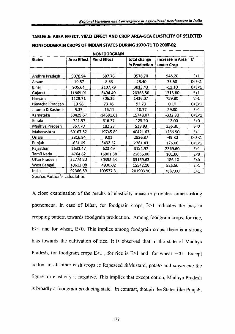
TABLE6.6: AREA EFFECT, YIELD EFFECT AND CROP AREA-GCA ELASTICITY OF SELECTED

NONFOODGRAIN CROPS OF INDIAN STATES DURING 1970-71 TO 200J-Oi

NONFOODGRAIN States Area Effect Yield Effect total change increase in Area E'


Andhra Pradesh 9070.94 507.76 9578.70 945.20 E>1

Assam -19.87 -8.53 -28.40 73.50 O<E<1 Bihar 905.64 2107.79 3013.43 -11.10 O<E<1 Gujarat 11869.01 8494.49 20363.50 1315.80 E>1 Haryana 1129.71 306.36 1436.07 759.80 E>1 Himachal Pradesh 19.58 73.16 92.73 0.10 O<E<1 Jammu & Kashmir 5.35 -16.11 -10.77 29.80 E>1 Karnataka 30429.67 -14681.61 15748.07 -332.90 O<E<1 Kerala -741.57 616.37 -125.20 -12.00 E<O Madhya Pradesh 357.70 182.23 539.93 356.30 E<O Maharashtra 60167.52 -19745.89 40421.63 1266.50 E>1 Orissa 2816.94 9.93 2826.87 -49.80 O<E<1 Punjab -651.09 3432.52 2781.43 176.00 O<E<1 Rajasthan 2531.47 623.49 3154.97 2369.60 E>1 Tamil Nadu 4764.62 16901.38 21666.00 101.00 E<O Uttar Pradesh 32774.20 30395.43 63169.63 -186.10 E<O West Bengal 10612.08 4930.02 15542.10 825.50 E>1 India 92366.59 109537.31 201903.90 7887.60 E>1 Source:Author' s calculation

A close examination of the results of elasticity measure provides some striking

phenomena. In case of Bihar, for foodgrain crops, E> 1 indicates the bias in

cropping pattern towards foodgrain production. Among foodgrain crops, for rice,

E> I and for wheat, E<O. This implies among foodgrain crops, there is a strong

bias towards the cultivation of rice. It is observed that in the state of Madhya

Pradesh, for foodgrain crops E> 1 , for rice is E> 1 and for wheat E<O . Except

cotton, in all other cash crops ie Rapeseed &Mustard, potato and sugarcane the

figure for elasticity is negative. This implies that except cotton, Madhya Pradesh

is broadly a foodgrain producing state. In contrast, though the States like Punjab,

172


Tamil Nadu are broadly foodgrain dominated, there is observed to be a marginal

shift in cropping pattern towards the cultivation of non-food crops.

6.6 Measuring Diversity in cropping pattern Herfindal Index

The change in cropping pattern can further be analysed by using the indices of

crop diversification. There are different indices to measure the extent of crop

diversification like Herfindal Index, Simpson Index, Ogive Index and Entropy

Index etc. Among them Herfindal Index, Simpson Index and Entropy Index are

used widely. These indices are calculated on the basis of proportion of GCA under

different crop cultivated in a particular geographical area. Crop diversification

index is actually a measure to show the direction of change of cropping pattern of

a particular state or region at a point of time. The more the state is diversified in

cropping the more the change in cropping pattern is expected towards high value

crop.

In this study we have used the Herfindal Index to measure the pace of crop

diversification across states in India during the period 1970-71 to 2009-G&. The

computation of index enable us to make an interstate comparison about the extent

to which the states are able to diversify overtime and the question that whether the

agriculturally advanced states with better provision of irrigation, fertilizer and

assured supply of variety of input usage are able to diversify more than their

poorer counterpart. That means, is the rich-poor gap plays any role in crop

diversification?

173


Basically the nature of crop diversification is amenable to agro climatic

environment, weather condition, soil quality, temperature etc. Some crops are

better produced in the tropical zone whereas some are better produced in arid zone

and coastal area. So production of a crop is essentially dependent on the weather

condition of the particular region. Despite this, provision of assured irrigation, use

of HYV seeds, use of fertilizers may change the cropping pattern a lot.

Therefore, spatial variation in respect of supply of assured irrigation and others

plays a major role in crop diversification.

TABLE6.7: HERFINDAL INDEX OF CROP DIVERSIFICATION OF INDIAN STATES

1970-71 1980-81 1991-92 2000-o1 2007-o8

Andhra Pradesh 0.494 0.490 0.679 0.673 0.696

Assam 0.415 0.446 0.476 0.490 0.559

Bihar 0.192 0.557 0.355 0.176 0.210

Gujarat 0.717 0.749 0.849 0.885 0.827

Haryana 0.997 0.993 0.975 0.987 0.985

Himachal Pradesh 0.187 0.143 0.235 0.221 0.300

Jammu & Kashmir 0.200 0.261 0.295 0.334 0.341

Karnataka 0.556 0.605 0.661 0.595 0.626

Kerala 0.900 0.913 0.964 0.985 0.992

Madhya Pradesh 0.327 0.655 0.561 0.695 0.692

Maharashtra 0.531 0.528 0.574 0.596 0.638

Orissa 0.531 0.376 0.454 0.557 0.629

Punjab 0.516 0.478 0.428 0.371 0.352

Rajasthan 0.407 0.493 0.593 0.644 0.612

Tamil Nadu 0.503 0.567 0.668 0.608 0.711

Uttar Pradesh 0.272 0.447 0.373 0.354 0.405

West Bengal 0.253 0.352 0.448 0.531 0.568


174


In this section the Herfmdal Index is computed for each state for the years 1970-

71, 1980-81, 1990-91, 2000-01 and 2007-08 respectively. The result of the

calculated HH Index is presented in the table 6.7. HHI is basically a concentration

index and thus the higher value is an indicator of specialization of crop activities.

So, to obtain the index of diversification it is subtracted from 1. The index value

above 0.5 mentions that the crop diversification is high while the value below 0.5

means the reverse that is the rate of crop diversification is slow. In other words it

means concentration or specialization in some crops.

From the result it is obvious that the states like Kerala, Gujarat, Kamataka,

Maharashtra, Madhya Pradesh and Tamil Nadu were able to diversify their crop

from the beginning of the period. Crop diversification is higher in these states.

Further, the states Andhra Pradesh and Rajasthan hastened the process of crop

diversification from the reform period. The same is true for the state West Bengal

from the year 2000-01. The state of Assam began this process recently as the

index value surpassed 0.5 for this state in 2007-08. Moreover, the state of Orissa

initially being diversified slowed down in later years. But since 2000-01 the

process of diversification has started again. On the other hand, the rate of crop

diversification has been slow in the states like Bihar, Himachal Pradesh, Jammu

&Kashmir, Punjab, and Uttar Pradesh. Otherwise it can be said that the above

states are concentrated in the production of some selected crops. Crop

concentration is high for these states. In fact, these states are mainly foodgrain

based.

175


6.7 Regional Disparity in Agricultural Infrastructure In India: An

Interstate Analysis

India is characterized by wide regional variation m agro-climatic condition.

Output in different region is varied due to varied agro-climatic factors, physical

resource endowment and also varying level of investment in rural infrastructure

and technological innovation. After the advent of new seed fertilizer technology

the improvement in growth in output and yield per hectare in India became

dependent more on irrigation condition, use of inputs i.e. use of fertilizers,

tractors, pumpsets, rural electrification etc. The use of HYV seeds is very much

amenable to the fertilizers and irrigation. The states with better irrigation status

got better results in yield growth than the states with poorer irrigation condition.

The correlation coefficient between yield growth and the quantum and intensity of

inputs used is found to be strong.

This study attempts to examine the disparities prevailing in the use of various

agricultural inputs across states and to investigate the regional variation in

agricultural development. A composite index of agricultural infrastructure has

been constructed by 'Deprivation Method' to explore the disparity in agricultural

infrastructure across the states of India. The detailed methodology of constructing

the index is explained in the chapter 3 {pg-53-55).

For constructing this index eight agricultural development indicators are selected.

They are following

);>Cropping intensity (CI)

);>Percentage irrigated area to GCA(IAGC)

176


~Fertilizer consumption per hectare of GCA ( fcgc)

~Credit to agriculture (CCA)

~Number of tractors and pumpsets used per 1 000 hectares (TAP)

~Average yield of agricultural land (A Y)

~Road length per 100 sq km (RL)

~Percentage share to total consumption of electricity in agriculture (CELA)

The regional variation in the use of agricultural inputs in India is quite high. A

close examination of the statistics of few selected indicators reveals this striking

phenomenon. Use of fertilizer per hectare varies from 44.41 to 215.73 Kg/beet in

the year 2007-08. The percentage of area irrigated to GCA varies from 2.4

hectare in Assam to 97.7 hectare in Punjab in the same year. In per capita credit to

agriculture the state of Jammu& Kashmir lagged far behind the other states in

India during the period 1981 to 2008. There is a substantial difference in the

percentage use of electricity for agriculture purpose across states. It varies from

0.53% in HP to 40.17% in Haryana . Further, there remains a huge gap across

states in road length in km per hundred square Km.

In order to make an account of whether regional variation across states has

widened overtime in terms of the selected development indicators, two measures

of inequality are employed. They are Coefficient of variation (COV)4 and Gini

concentration coefficient (GINIC) 5.

4 (SD/Mean) * I 00 5

GiniC= 2Cov(y,r)IN y (see Pyatt eta!., 1980)

177


TABLE6.8: INEQUALITY MEASURES OF AGRICULTURAL INFRASTRUCTURE INDICATORS

DURING THE PERIOD 1981,1991,2001 AND 2007

Coefficient of Variation GINIC

1981 1991 2001 2007 1981 1991 2001 2007

Cl 0.137 0.151 0.163 0.302 -0.075 -0.082 -0.088 -0.139

IAGC 0.668 0.635 0.620 0.617 -0.336 -0.319 -0.334 -0.337

FCGC 0.832 0.603 0.535 0.496 -0.403 -0.330 -0.293 -0.273

CCA 0.733 0.652 0.713 0.677 -0.400 -0.358 -0.395 -0.375

TAP 1.161 1.064 0.862 0.858 -0.540 -0.505 -0.419 -0.030

AY 0.400 0.496 0.434 0.405 -0.213 -0.265 -0.232 -0.224

RL 0.903 0.923 0.855 0.962 -0.378 -0.391 -0.381 -0.100

CELA 0.891 0.701 0.762 0.749 -0.478 -0.388 -0.419 0.211


The results of the computed coefficient of variation and GINIC measures are

presented in the table 6.8. The COV and GINIC measures have provided more or

less identical results in exhibiting the inequality trend across states in terms of the

selected development indicators. For cropping intensity and road length in km per

100 sq km a sharp rising trend is observed in both COV and GINIC for the whole

period (1980-81 to 2007-08). Fortunately, in the factors like percentage irrigated

area to GCA,. fertilizer consumption per hectare of GCA, credit to agriculture,

number of tractors and pumpsets used per 1 000 hectares, percentage share to total

consumption of electricity in agriculture, the inequality measures have shown a

downward trend for overall period. Only the factor average yield shows a

fluctuating trend during the time period.

178


Though it has been revealed by the inequality measures that disparity in terms of

the above mentioned development indicators are diminishing across states

overtime but the formation of index would reveal actually whether it is possible

for any agriculturally poor state to catch up or going ahead of a agriculturally

developed states over the chosen period of time. The computed index of all the

states and the subsequent rank of each state according to the value of the index are

presented in the table 6.9 for the year 1980-81, 1990-91, 2000-01 and 2007-08

respectively. From the ranking of the index appearing in the table it is apparently

clear that the states which was in topmost position in 1980-81 are still remaining

in the same position in the year 2007-08 ie the states occupying the top five

position in 1980-81 are successful to maintain the similar position in the year

2007-08 whereas Assam and Orissa remained as two least developed states

throughout the whole period. Other than these seven states, it has been observed

for few states to change their position in the course of time. For example the state

of Madhya Pradesh being in the lowest position in 1980-81 staged up to lth

position in 2007-08. Again the state Kamataka and Himachal Pradesh being in the

same position in 1980-81 went to different destinations in 2007-08, while

Kamataka triggered to achieve a position of 9th in 2007-08, Himachal Pradesh

trailed behind by getting a position of 15th among the 17 states in the same year.

Moreover, the performance of Jammu& Kashmir has been remained poor

throughout the period. Its position deteriorated from 9th in 1980-81 to 14th in the

terminal year. Also it is noticeable that West Bengal being in the position 11 in

1980-81 improved its performance to reach a position ofih in 2007-08.

179


TABLE6.9: COMPOSITE INDEX OF AGRICULTURE INFRASTRUCTURE OF INDIAN

STATES DURING 1980-81 TO 2007-08 (CIAI)

INDEX RANK 1980- 1990- 2000- 2007- 1980- 2000- 2007-81 91 01 08 81 1990-91 01 08

AndhraPradesh 0.33 0.52 0.57 0.58 5 4 4.5 4

Assam 0.10 0.10 0.10 0.08 16.5 17 17 16 Bihar 0.21 0.29 0.39 0.39 11 8.5 8 8 Gujarat 0.28 0.31 0.32 0.45 7 7 10 6 Haryana 0.60 0.72 0.73 0.76 2 2 2 2 Himachal Pradesh 0.17 0.17 0.16 0.16 13.5 15 15 15 Jammu&Kashmir 0.22 0.22 0.20 0.23 9 12.5 14 14 Karnataka 0.17 0.33 0.41 0.37 13.5 6 7 9 Kerala 0.31 0.28 0.33 0.27 6 10 9 13 Madhya Pradesh 0.10 0.21 0.22 0.31 16.5 14 13 12 Maharashtra 0.21 0.26 0.28 0.32 11 11 11 11 Orissa 0.12 0.13 0.12 0.07 15 16 16 17 Punjab 0.90 0.94 0.85 0.85 1 1 1 1 Rajasthan 0.24 0.22 0.27 0.34 8 12.5 12 10 TamiiNadu 0.51 0.50 0.57 0.54 4 5 4.5 5 UttarPradesh 0.53 0.61 0.61 0.63 3 3 3 3 WestBengal 0.21 0.29 0.42 0.41 11 8.5 6 7


Thus the fact: is that contrary to agriculturally poor states, some agriculturally

advanced states have been successful in creating agricultural infrastructures and

thus they are enjoying the benefits of modem agricultural development. This

resulted in the prevalence of disparities across states

6.8 Agricultural Growth in India: A Convergence Analysis

This section deals with the convergence analysis of per capita value of agricultural

output during the period 1970-71 to 2008-09. Following Barro and Salai- Martin's

notions of convergence, sigma convergence and ~ convergence of PCVOA have

been measured. Again in order to measure the factors that are responsible for

creating divergence across states, conditional convergence tests are performed.

180


Using dynamic panel data model, the regression analysis for testing conditional

convergence has been done using the Generalized Method of Moments technique.

Moreover, to specify the states that are responsible for overall divergence or the

states that are not converging to national average, unit root test has been

performed.

The analysis of growth rate of total value of agricultural output and yield for

Indian states during the period reveals the fact that on an average value of output

for the country grew at the rate of 2.6% whereas the yield grew at a rate of 1.43%

for the whole period. The segregation of the whole period into three phases reveal

that during the post green revolution period both output and yield growth

accelerated but in the post reform period growth rate decelerated for the country

as well as for majority of the states. Moreover, the growth rate achieved at the

national level is not uniform across the states. After the initiation of Green

Revolution disparity among states has, in fact, increased at a high rate. Some

Western and Eastern states got the benefit of better irrigation, sufficient rainfall,

good soil quality etc initially. But after sometime good effects of Green

Revolution spread to all over India and disparity somewhat diminished. After the

introduction of New Economic Reform, in the neoliberal regime, inequality again

started increasing. The estimation of coefficient of variation of value of

agricultural output for the states show that coefficient of variation increased from

0. 79 in 1970-71 to 0.95 in 2002-03 and again marginally dropped to 0.89 in 2005-

06, still it is much higher than the level in 1970-71.

181

c: 0 ·.;::;

"' ·;:

"' > -0 .... c: <II ·;::; :;:: -<II 0 u


Coefficient of variation of total and per capita value of output

100 90 80 70 60 50 40 30 20 10

0

AT1/ , ._.,...,~ - .

.-t <:t l' o rY'l lDC'lNU'lOO .-t <:tl' ~~r:--ooD?~~q'~c;'9 9 9 OrY'l<Dcf.,NLI'lOO.-t<:ti' O rY'llD r--r--r--,..._oooooommmooo 0'\0'\ C'lC'IC'lC'lO'\C'lC'lmOO O ~MM MMMMMHMr-.JNN

Figure 6.2

- per ca pita va lue of output

- total va lue of output

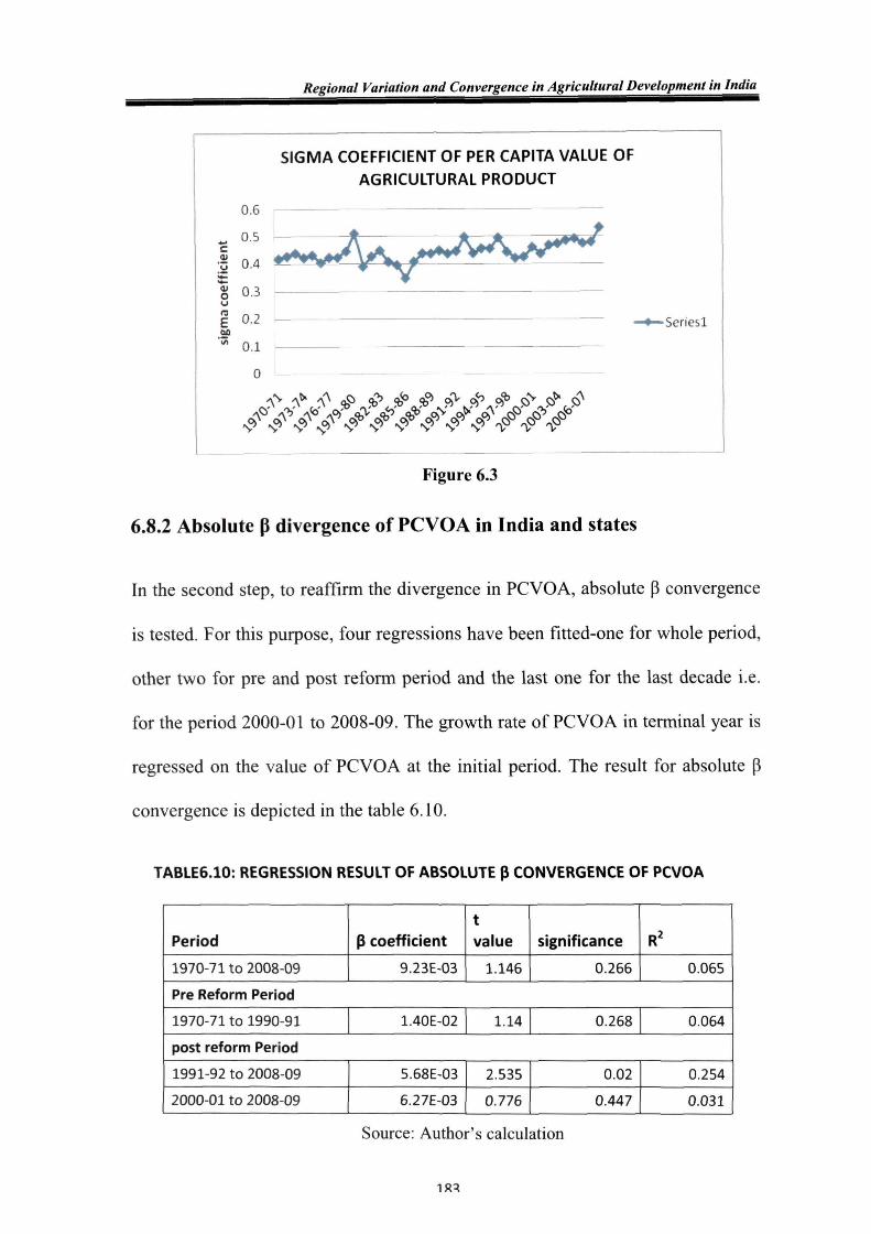
6.8.1 Sigma Convergence of PCVOA across states of India

Next, an attempt has been made to examine the nature of divergence/convergence

of per capita value of agricultural output in Indian states. In this regard, first of all

we have tested the sigma convergence for PCVOA across states overtime. The

result is displayed in figure 6.3. The figure plots standard deviation of logarithm

of PCVOA of states for the period 1970-71 to 2008-09. The standard deviation

increased from 0.4 in 1970-71 to 0.53 in 2008-09 indicating a trend of divergence.

In the figure it is observed that during 1975-76 disparity increased considerably

but it slowed down during 80's ie in the second phase of green revolution but

from the year 1991-92 it again picked up and continued to rise till 2008-09. In

other words, the test of sigma convergence confirms the divergence of per capita

value of agricultural output across Indian states over time.


0.6

SIGMA COEFFICIENT OF PER CAPITA VALUE OF AGRICULTURAL PRODUCT

~ o.s~-~ ·;:; 0 .4 y :;:: -~ 0.3 u ro E 0.2 -+-Series l till

·u; 0.1

0

Figure 6.3

6.8.2 Absolute ~ divergence of PCVOA in India and states

In the second step, to reaffirm the divergence in PCVOA, absolute ~ convergence

is tested. For this purpose, four regressions have been fitted-one for whole period,

other two for pre and post reform period and the last one for the last decade i.e.

for the period 2000-01 to 2008-09. The growth rate ofPCVOA in terminal year is

regressed on the value of PCVOA at the initial period. The result for absolute ~

convergence is depicted in the table 6.1 0.

TABLE6.10: REGRESSION RESULT OF ABSOLUTE p CONVERGENCE OF PCVOA

t Period p coefficient value significance R2

1970-71 to 2008-09 9.23E-03 1.146 0.266 0.065

Pre Reform Period

1970-71 to 1990-91 1.40E-02 1.14 0.268 0.064

post reform Period

1991-92 to 2008-09 5.68E-03 2.535 0.02 0.254

2000-01 to 2008-09 6.27E-03 0.776 0.447 0.031



The results indicate absolute divergence for all the four periods. Absence of

absolute convergence in PCVOA calls for examination of conditional

convergence.

6.8.3 Conditional p convergence in PCVOA in India

We have estimated the dynamic panel data model by GMM methods. In

explaining divergence in agriculture across states, we have chosen explanatory

variables as the rainfall of different states, composite index of agricultural

infrastructure and literacy rate. It is to be noted that <b~.oS~index is an weighted

index computed from an array of infrastructural variable in agriculture across

states. These are - Cropping intensity (CI), percentage irrigated area to GCA

(IAGC), fertilizer consumption per hectare of GCA (Fertc) credit to agriculture

(CCA), number of tractors and pumpsets used per 1000 hectares (TAP), average

yield of agricultural land (A Y), road length per 100 sq km (RL ), percentage share

to total consumption of electricity in agriculture (CELA). It is mentioned in

previous sections that the weights are determined by applying PCA for the

variables. The use of CIAI facilitates us from avoiding the problem of

multicollinearity. In the present section we use the panel of four years for the

entire period (1980-81 to 2007-08). There are 7 panels. The total number of

observation for 16 states becomes 112 and the GMM estimation method is used.

The regression equation that has been fitted here is

184


In the GMM estimation analysis (see table 6.11), the coefficient of 1+~ becomes

0.104 ie the estimated coefficient of~ is -0.896 which is significant at 10% level.

This implies conditional ~ convergence. It is revealed from the result that the

coefficient of CIAI is positive and highly significant. This implies clearly that the

factors determining the condition of agricultural infrastructure which are the main

backbone of agricultural development are significantly responsible for widespread

divergence in agriculture across states of India. It has been also observed from the

result that the coefficient on rainfall is positive and significant. It is an expected

result as rainfall has a significant role to play in agriculture. Variations in rainfall

create divergence among states. Moreover, the coefficient of literacy rate is also

significant but at 14% level. The speed of convergence is 0.224 which is also

high. Thus the result of conditional convergence in case ofPCVOA among Indian

states implies that states are converging to their own steady states. Actually the

states are converging to divergent steady states. It can be said that the index of

agricultural infrastructure acts as a package of agricultural infrastructure across

states and thus play a significant role in explaining divergence in PCVOA.

TABLE6.11: RESULT OF GMM ANALYSIS WITH DETERMINANT CIAI, RAIN AND LITERACY RATE

DURING THE PERIOD 198o-81 TO 2007-08

Variable Coefficient t-Statistic Prob.

PCVOA(-1) 0.104089 1.346821 0.182

CIA I 1.356878 3.277818 0.0016

RAIN 0.000136 7.519695 0

LIT 0.002709 1.476619 0.1439

Source :Author' scalculation

Note: On the availability of comparable figures for the chosen variables, 16 states have been

identified and compiled data over a period of 28 years 1980-81 to 2007-08

185


However, the composite index of agricultural infrastructure (CIAI) encompasses

several indicators of agricultural development. As observed in India, the

variability in agricultural production is mainly responsible to the variations in

agricultural inputs like rainfall, use of fertilizers and irrigation intensity.

Accordingly a renewed attempt has been taken to examine the role of these

individual indicators on the convergence or divergence of agricultural output over

the period 1970-71 to 2007-08 in Indian agriculture.

Using the same equation of regression, we again consider in this case the panel of

four years with 17 states for the period 1970-71 to 2007-08, there are 9 panels and

therefore total number observation becomes 153.

TABLE 6.12: RESULT OF GMM ANALYSIS WITH DETERMINANT RAIN,FERTC,IA AND LIT

DURING THE PERIOD 1970-71 TO 2007-08

Variable Coefficient t-Statistic Pro b. PCVOA(-1) 0.563143 6.701233 0 RAIN 0.268853 6.450424 0 FERTC 0.297185 3.168496 0.002 lA -0.133 -1.5255 0.1299 LIT -0.51982 -3.11569 0.0023

Source:Author' scalculation

Note: On the availability of comparable figures for the chosen variables, 17 states have been identified

and compiled data over a period of 3 8 years 1970-71 to 2007-08

The result (see table 6.12) of the estimation analysis reveals that the estimated

coefficients for ~ is negative ie (-0.437), (1+~=0.563) confirming further

conditional convergence. The coefficient of rain and fertilizer are found to be

positive and significant. Only the coefficient of the factors IA and literacy bears a

negative sign. This may be is attributable to the problem of multicollenearity. This

186


result implies that supply of input is also a major factor of explaining divergence

in per capita value of agricultural output.

Thus, overall it can be asserted that absolute divergence in PCVOA across states

of India can be rectified and convergence of states can be possible if proper

infrastructure in agriculture can be set up in agriculturally backward states and

thereby the gap can be reduced. In this connection it is also the fact that the

uneven distribution of input is creating a major barrier in bringing a converging

outcome in agricultural production across states.

6.8.4 Unit root test of Divergence: An Interstate Analysis

Historically, the conventional cross sectional regressiOn for determining

convergence has come under criticisms (Quah, 1993, Friedman, 1992). Quah

showed that this bias is similar to Galton's Fallacy whereas Friedman comments

that convergence is indicated by a diminution of the variance among countries

overtime. Several studies now relied on time series information for determining

the existence or lack there of of convergence rather on cross

section.(BenDevid,1993,1994, Bernard and Duarlof,l995,1996), Li and

Papell,1999, Cheung and Pascual,2004). Long run forecast of difference between

any pair of countries PCGDP converges to zero as the forecast horizon grows

according to this new methodology. Within a neoclassical set up the test for

convergence of per capita income is translated to a test for the stationarity of

output differential (see chapter3 for methodology, pg-49-50).

187


In this context we examine in this section the behavior of each state's per capita

agricultural output differential with the national average overtime and to ascertain

whether there is any noticeable evidence of convergence over time.

The statistical tests of long run convergence hinges on the time series properties

of [In(Yi,t)-In(-Y •t)] where In(Yi,t) and In(-Y •t) are respectively the logarithm of

per capita value of output of ith state and the national average. In this section the

behavior of [In(Y i,t)-In(-Y •t)] has been tested for the period 1980-81 to 2008-09

for 18 states.

TABLE 6.13: PHILIPS-PERRON UNIT ROOT TEST FOR CONVERGENCE OF PCVOA OF

INDIAN STATES

State PP Test Statistics P-value Andhra Pradesh -4.6* 0

Arunachal Pradesh -2.84 0.19

Assam -5.27* 0

Bihar -3** 0.14

Goa -5.78* 0

Gujarat -4.68* 0

Haryana -4.15 0.01

Himachal Pradesh -4.28* 0

Jammu & Kashmir -2.79 0.2

Karnataka -3.7** 0.03

Kerala -2.42 0.36

Madhya Pradesh -1.82 0.36

Maharashtra -4.18** 0.01

Manipur -3.77** 0.03

Orissa -4.89* 0.002

Punjab -4.16 0.01

Rajasthan -6.37* 0

Tamil Nadu -3.48** 0.01

Uttar Pradesh -4.19** 0.01

West Bengal -2.56 0.29

Notes:* and** denote significance at 1 and 5 percent level respectively


188

Regional Variation and Convergence in Agriculturel Development in India

The result of the unit root test for convergence shows a diverging pattern across

states in case of agricultural output. The result is depicted in the table 6.13. The

null hypothesis of unit root for Phillips Pheron test is rejected for the states

Andhrapradesh,Assam, Goa,HimachalPradesh,Kamataka,Maharashtra,Manipur, Or

issa,TamilNadu,UttarPradesh whereas the existence of unit root is accepted for the

states Arunachal Pradesh, Bihar, Jammu& Kashmir, Kerala, Madhya Pradesh,

Punjab, Haryana and West Bengal. Therefore, while 10 states are converging

towards national average in PCVOA overtime, the 8 states are following a

different steady state from national average. Interestingly, out of eight states three

states like Punjab, Haryana and West Bengal belong to the category of

agriculturally advanced states while the remaining five states Arunachal Pradesh,

Bihar, Jammu& Kashmir, Kerala and Madhya Pradesh belong to the category of

backward states. Thus our results establish the argument that the wide variety in

agricultural infrastructure among these eight states is responsible for wide

variability in agricultural production and thus making the growth path divergent.

6.9 Analysis of possible reasons for divergence in PCVOA in India

In the preceding analysis it has been observed that the crucial detenninants of

difference in agricultural growth across states of India are agricultural

infrastructure, rainfall as well as individually irrigated area, consumption of

fertilizer, rainfall. The index of agricultural infrastructure has been constructed

taking into account an array of relevant infrastructural variables. It can be said that

the development of agricultural infrastructure is one of the basic responsibility of

the state government. A substantial amount of public investment is required for

the development of agricultural infrastructure. In order to infer about the

189


distribution of public investment in agriculture across states, the proxy for public

investment ie PCCE has been regressed on CIAI in the fixed effect framework.

The result (see table 6.14) shows a statistically significant positive relationship

between the two.

TABLE 6.14: RELATION BETWEEN GOVERNMENT EXPENDITURE AND AGRICULTURE

INFRASTRUCTURE ACROSS STATES IN INDIA

Variable Coefficient t-Statistic Pro b.

c 2.197639 3.868587 0.0002

CIAI 9.194107 6.002615 0


This implies that the distribution of public investment has been made in favour of

agriculturally developed states. Again to know about the distribution of private

investment in agriculture PCLS has been regressed on CIAI. The positive and

significant relation ensures that private investment 1s also biased towards

agriculturally developed states (see table 6.15). It 1s obvious that private

investment is also generally flows to the states where returns would be high. So

making investment in already developed states would be profitable. Therefore the

skewed distribution of public investment along with difference in weather is the

possible reasons for agricultural divergence in Indian states.

TABLE 6.15: RELATION BETWEEN PRIVATE EXPENDITURE AND AGRICULTURE

INFRASTRUCTURE ACROSS STATES IN INDIA


c 4.185833 7.27191 0

CIA I 4.005533 2.580844 0.0113


190


Some recent studies by Yang and Zhu (2004) and Tiffm and Irz (2006) find

agriculture as an important cause for economic growth and conclude that

economic growth cannot be sustained without improving agricultural productivity.

To enquire about whether the regional difference in agricultural infrastructure has

any role to play in explaining divergence in PCNSDP, PCNSDP is regressed on

CIAI (see table 6.16).

TABLE 6.16: RELATION BETWEEN PCNSDP AND AGRICULTURE INFRASTRUCTURE

ACROSS STATES IN INDIA


c 4.657447 1.907901 0.0651

CIAI 11.85005 1.901838 0.066


It is established from regression result that PCNSDP is high where CIAI is high.

This implies a better developed agricultural infrastructure would enhance

PCNSDP of a state. Thus a broad based developed agriculture can contribute to

higher economic growth of a region. It is stated in a study (Johston & Mellor

1961) that linkages of agriculture within the agriculture sector and with the

nonagricultural sectors are crucial to economic growth.

6.10 Summery and Conclusion

In this study an attempt has been made to examine the performance of major

Indian states in respect of agricultural output and thereby disparity prevailing

across the states. The growth rates of agricultural output clearly reveal the fact

that Indian agriculture has passed a phase of outstanding growth during 80's, but

191


after New Economic Reform the growth momentum has taken a downturn. For

the overall period the states like Haryana, Maharashtra, Rajasthan, West Bengal,

Goa, Himachal Pradesh, Madhya Pradesh, Manipur and Punjab performed well in

terms of growth of value of agricultural output. The kinked growth rate in the

second phase of green revolution reveals that all the states made a remarkable

progress during this period. The best performed states during this period were

Tamil Nadu, West Bengal, Rajasthan, Punjab and Haryana. The states like Bihar,

Orissa, Kerala, Himachal Pradesh and Assam also registered significant

improvement during this period. But the growth performance during the post

reform period experienced a severe slowdown in respect of growth of agricultural

output. The country as well as the states decelerated during the post reform

period. The similar trend was followed in case of yield growth also.

This study also attempts to analyse the cropping pattern of India as well as states

during the period 1970-71 to 2007-08 by looking into the area allocation and crop

area- GCA elasticity. The cropping pattern in India is mainly biased towards

foodgrain crops. But a change in cropping pattern is observed in favour of some

nonfoodgrain crops during the study period. This study reveals that except Punjab

and Bihar the area allocation towards foodgrain crops decreased for all the states

during the study period. In case of non-foodgrain crops the states like Andhra

Pradesh, Gujarat, Haryana, Jammu& Kashmir, Madhya Pradesh, Maharashtra,

Rajasthan, Tamil Nadu and West Bengal experienced an increasing trend of crop

diversification. Moreover, the elasticity measures also imply the similar pattern of

crop diversification for the states as well as for the country. At the country level

192


elasticity for foodgrain is negative whereas for nonfoodgrain crops it is positive

and greater than one implying a diversion of area allocation towards nonfoodgrain

crops at a higher rate than the change in GCA. In order to explore the actual

extent of crop diversification Herfindal Index has also been computed for the

period 1970-71 to 2008-09. The result confirms that the food grain dominated

states scores low in the crop diversification index and the states like Andhra

Pradesh, Assam, Gujarat, Haryana, Kamataka, Kerala, Madhya Pradesh,

Maharashtra, Orissa, Rajasthan, Tamil Nadu and West Bengal scored high in

Herfindal Index.

In this study attempt has also been made to measure the disparity across states in

terms of agricultural infrastructural factors. The factors like cropping pattern and

road length per 100 sq km indicate an increasing trend in disparity over the period

whereas for the other factors like irrigated area, consumption of fertiliser,

disparity is reducing. In order to analyse the position of states in terms of their

agricultural endowment a composite index has been constructed encompassing

eight agricultural infrastructural indicators .. This index reveals the true picture of

disparity exhibiting that except some exception the states that get proper

agricultural infrastructure during 80's remained at top still in the period of 2007-

08 whereas some weaker states Assam and Orissa lagged behind in getting proper

agricultural infrastructure throughout the period.

An attempt has also been made in this study to analyse convergence or divergence

of per capita value of agricultural output. The conventional cross section ~ and a

coefficient testing confirm that there is absolute divergence and interstate

193


disparity increased during the period. The analysis in dynamic panel data model

also supports the result of absolute ~ divergence in per capita value of agricultural

output during the period 1970-71 to 2007-08. The result of absolute P divergence

calls for the testing of conditional convergence of per capita value of agricultural

output for the specified period. As mentioned in the study the conditional

convergence testing is performed twice taking into account two different vectors

of independent variables. The conditional convergence is confirmed in both cases.

This result indicates that Indian agriculture is characterized by significant regional

variation in respect of provision of agricultural infrastructure. If this gallant

infrastructural gap in agriculture can be combated then there will certainly be a

convergence across states in agriculture in India. Similarly the significant regional

disparity in respect of assured irrigation, supply of fertilizers as well as literacy

should be reduced to bring into convergence in agriculture in India. However, the

Philips-Perron unit root test reveals that 10 out of 18 states are converging

towards national average whereas the 8 remaining states maintaining a diverging

trend from national average in terms of per capita value of agricultural output.

Thus it can be said in conclusion that performance of states in terms of

agricultural production and yield is lacking the significant acceleration in growth

in recent period which was observed during 80~s. Some economists suggest for

second green revolution for bringing an accelerated performance in agricultural

output and yield in India. But important findings of conditional convergence

reassures that without an inclusive improvement of agricultural infrastructure ,

accelerated development would not have been possible in Indian agriculture. To

194


mitigate the regional gap in agricultural infrastructure the policy prescription

would be more and more investment in the lagged region, extension of public and

private credit in remote rural areas. Development of research focusing the

development of dry land area, development of technology requiring less water,

less fertilizer and cheap farming and finally implementation of watershed

development approach are necessary for a more balanced and sustainable

agricultural development in the country.

195


APPENDIX

TABLE6AI: CHANGE IN CROPPING PATTERN OF INDIAN STATES DURING THE

PERIOD 1970-71 TO 2007-08

TABLE6AI1: CHANGE IN CROPPING PATTERN OF INDIAN STATES DURING THE PERIOD 1970-71 TO

2007-08 IN RICE

Table GAll: RICE

States 1970-71 1980-81 1990-91 2000-01 2007-08

ANDHRA PRADESH 26.4 29.4 29.8 31.3 29.4

ASSAM 71.0 66.0 65.5 65.4 60.5

BIHAR 47.8 34.3 45.8 45.9 45.2

GUJARAT 4.9 5.3 5.7 5.6 6.2

HARYANA 5.4 8.9 11.5 17.2 16.6

HIMACHAL PRADESH 10.5 11.6 8.5 8.6 8.1

JAMMU AND KASHMIR 25.6 27.2 25.2 21.9 23.2

KARNATAKA 10.7 10.5 10.2 12.1 11.0

KERALA 29.8 28.0 17.9 11.5 8.3

MADHYA PRADESH 21.3 7.1 8.7 9.4 7.6

MAHARASHTRA 7.0 7.2 7.7 5.6 6.9

ORISSA 53.4 47.9 46.3 56.3 49.4

PUNJAB 6.9 17.5 27.6 32.9 33.2

RAJASTHAN 0.7 1.0 0.8 0.9 0.6

TAMIL NADU 36.4 35.5 30.4 33.3 30.8

UTIAR PRADESH 19.7 20.0 21.4 23.1 22.9

WEST BENGAL 69.9 67.9 66.9 59.6 58.7

INDIA 22.5 22.9 23.4 23.9 22.4


196


TABLE6AI2:CHANGE IN CROPPING PATTERN OF INDIAN STATES DURING THE PERIOD 1970-71 TO

2007-08 IN WHEAT

WHEAT

1970-71 1980-81 1990-91 2000-01 2007-08

Andhra Pradesh 0.1 0.1 0.1 0.1 0.1

Assam 0.7 3.0 2.0 1.7 1.5

Bihar 11.9 15.1 23.9 26.4 27.3

Gujarat 5.7 5.8 3.9 2.7 10.4

Haryana 22.8 27.0 32.5 38.4 38.1

Himachal Pradesh 33.2 37.0 38.5 39.9 37.8

Jammu & Kashmir 21.2 20.3 22.9 24.8 24.5

Karnataka 2.8 2.9 1.6 2.2 2.1

Madhya Pradesh 16.5 15.2 19.8 15.0 18.3

Maharashtra 4.6 5.3 3.1 3.5 5.5

Orissa 0.2 0.8 0.3 0.1 0.1

Punjab 40.5 41.6 43.1 42.9 44.3

Rajasthan 8.8 9.4 9.8 12.0 11.7

Uttar Pradesh 25.5 31.1 34.3 36.2 36.6

West Bengal 5.1 3.7 2.9 4.7 3.6

India 10.9 12.9 12.8 13.5 14.3



2007-0SIN JUTE

JUTE

1970-71 1980-81 1990-91 2000-01 2007-08

Assam 4.7 3.3 2.6 1.7 1.6

Bihar 1.3 1.4 1.9 1.7 1.7

Orissa 0.5 0.5 0.4 0.0 0.1

West Bengal 5.7 8.0 6.7 6.7 6.3

India 10.9 12.9 12.8 13.5 14.3


197


TABLE6AI4:CHANGE IN CROPPING PATIERN OF INDIAN STATES DURING THE PERIOD 197G-71 TO

2007-08 IN COTION

COTTON

States 1970-71 1980-81 1990-91 2000-01 2007-08

Andhra Pradesh 2.4 3.4 5.4 7.5 8.4

Gujarat 15.7 14.6 10.8 15.5 19.3

Haryana 3.9 5.8 10.6 9.1 7.5

Karnataka 9.1 9.5 4.7 4.5 3.1

Kerala 0.3 0.2 0.4 0.1 0.0

Madhya Pradesh 3.4 2.8 3.2 2.6 3.1

Maharashtra 14.6 12.6 13.5 14.2 15.6

Orissa 0.0 0.0 0.1 0.5 0.6

Punjab 7.0 9.6 8.8 6.0 7.7

Rajasthan 1.3 2.1 2.6 2.7 1.7

Tamil Nadu 4.2 3.4 3.7 2.7 3.5

Uttar Pradesh 0.2 0.2 0.1 0.0 0.0

India 4.5 4.5 4.2 4.6 4.8


TABLE6AIS:CHANGE IN CROPPING PATIERN OF INDIAN STATES DURING THE PERIOD 1970-71 TO

2007-08 IN SUGARCANE

SUGARCANE States 1970-71 1980-81 1990-91 2000-01 2007-08 Andhra Pradesh 0.9 1.1 1.8 1.8 1.8 Assam 1.2 1.4 1.0 0.7 0.7 Bihar 1.5 0.9 1.8 1.2 1.4 Gujarat 0.4 0.9 1.1 1.7 1.7 Haryana 3.1 2.1 2.9 2.3 2.2 Himachal Pradesh 0.4 0.3 0.2 0.3 0.3 Jammu&Kashmir 0.4 0.3 0.2 0.3 0.3 Karnataka 0.9 1.4 2.3 3.4 2.4 Kerala 0.3 0.3 0.3 0.1 0.1 Madhya Pradesh 0.3 0.3 0.3 0.3 0.4 Maharashtra 1.1 1.3 2.2 2.8 5.4 Orissa 0.4 0.8 0.4 1.3 0.2 Punjab 2.3 0.7 1.4 0.3 0.3 Rajasthan 0.2 0.2 0.2 0.1 0.0 TamiiNadu 1.8 2.8 3.4 5.0 6.1 UttarPradesh 5.8 5.5 7.6 7.7 8.7 WestBengal 0.5 0.2 0.2 0.2 0.2 All India 1.6 1.5 2.1 2.3 2.6


198



2007-0SIN RAPESEED AND MUSTARD

RAPESEED & MUSTARD

States 1970-71 1980-81 1990-91 2000-01 2007-08

Assam 4.9 6.2 7.9 6.7 6.1

Bihar 0.8 0.6 1.1 1.3 1.1

Gujarat 0.3 1.6 3.7 1.8 2.8

Haryana 2.6 5.5 11.5 6.6 9.3

HimachaiPradesh 0.4 0.6 0.9 1.1 0.9

Jammu&Kashmir 2.9 4.1 5.5 5.7 5.0

Karnataka 0.1 0.0 0.0 0.1 0.0

Madhya Pradesh 1.0 0.8 3.2 2.5 2.8

Maharashtra 0.0 0.0 0.0 0.0 0.0

Orissa 0.7 1.9 1.8 0.2 0.2

Punjab 1.8 1.9 1.5 0.7 0.4

Rajasthan 1.5 2.1 13.2 8.0 11.2

UttarPradesh 9.3 1.7 3.5 3.6 3.5

West Bengal 1.5 1.7 4.8 4.8 4.2

All India 2.0 2.3 3.6 2.4 3.0



2007-0SIN POTATO

POTATO States 1970-71 1980-81 1990-91 2000-01 2007-08

Assam 0.9 1.1 1.6 2.0 2.0 Bihar 0.9 0.9 1.7 1.9 1.9 Gujarat 0.0 0.1 0.2 0.3 0.6 Haryana 0.1 0.2 0.2 0.3 0.3 Himachal Pradesh 1.9 1.4 1.5 1.4 1.4 Karnataka 0.1 0.1 0.2 0.3 0.5 Madhya Pradesh 0.1 0.1 0.2 0.2 0.2 Maharashtra 0.1 0.1 0.1 0.1 0.1 Orissa 0.2 0.1 0.1 0.1 0.1 Punjab 0.3 0.6 0.4 0.8 1.0 Rajasthan 0.0 0.0 0.0 0.0 0.0 Tamil Nadu 0.2 0.2 0.1 0.1 0.1 UttarPradesh 0.7 1.1 1.5 1.6 2.0 WestBengal 0.9 1.5 2.7 3.3 4.1 All India 0.3 0.4 0.6 0.7 0.8


199


TABLE 6AII: AREA EFFECT, YIELD EFFECT AND ELASTICITY OF

INDIAN STATES DURING THE PERIOD 1970-71 TO 2007-08

TABLE 6AIIl: AREA EFFECT, YIELD EFFECT AND ELASTICITY OF INDIAN STATES IN RICE DURING THE

PERIOD 1970-71 TO 2007-08

RICE



Andhra Pradesh -1163.59 10587.19 9423.60 462.80 E>1

Assam 321.02 961.65 1282.67 356.00 0<E<1

Bihar -206.56 708.72 502.17 -1702.10 E>1

Gujarat 281.24 424.16 705.40 270.40 E>l

Haryana 2176.72 661.28 2838.00 806.00 E<O

Himachal Pradesh 3.40 -5.96 -2.57 -16.60 E<O

Jammu & Kashmir 57.28 83.82 141.10 41.20 O<E<1

Karnataka 641.13 939.87 1581.00 256.00 E<O

Kerala -1060.94 383.44 -677.50 -646.20 E<O

Madhya Pradesh 5724.23 -7925.13 -2200.90 -2824.10 E>1

Maharashtra 116.47 504.53 621.00 218.00 E>1

Orissa -48.48 2656.62 2608.13 -59.20 O<E<l

Punjab 7159.23 2286.77 9446.00 2220.00 E>l

Rajasthan -59.93 120.07 60.13 8.80 O<E<l

Tamil Nadu -1893.91 2977.84 1083.93 -896.80 E>1

Uttar Pradesh 1461.86 6184.80 7646.67 1146.00 E>1

West Bengal 1428.11 7469.19 8897.30 759.70 O<E<l

India 10540.06 46414.94 56955.00 6322.40 O<E<1


200


TABLE 6AII2: AREA EFFECT, YIELD EFFECT AND ELASTICITY OF INDIAN STATES IN WHEAT DURING

THE PERIOD 1970-71 TO 2007-08

WHEAT



ANDHRA PRADESH -0.47 0.17 -0.30 -7.90 E<O

ASSAM 43.62 18.82 62.43 35.30 E>1

BIHAR 1052.07 1926.33 2978.40 846.90 E<O

GUJARAT 686.10 967.10 1653.20 696.80 E>1

HARYANA 4029.74 4988.26 9018.00 1333.00 E>1

HIMACHAL PRADESH 77.24 180.82 258.07 64.60 E>1

JAMMU AND KASHMIR 117.92 203.28 321.20 94.30 E>1

KARNATAKA 430.60 -328.33 102.27 -29.00 O<E<1

MADHYA PRADESH 749.80 3125.20 3875.00 339.30 E<O

MAHARASHTRA -207.08 1272.08 1065.00 371.00 E>1

ORISSA -11.51 -1.16 -12.67 -7.40 O<E<1

PUNJAB 3433.32 6358.01 9791.33 1189.00 E>1

RAJASTHAN 1470.73 3126.84 4597.57 1113.80 E>1

UTIAR PRADESH 5943.68 11127.65 17071.33 3208.00 E>1

WEST BENGAL 116.44 -219.94 -103.50 -7.40 E<O

INDIA 16671.52 40176.48 56848.00 9797.60 O<E<1


TABLE 6AII3: AREA EFFECT, YIELD EFFECT AND ELASTICITY OF INDIAN STATES IN JUTE DURING THE

PERIOD 1970-71 TO 2007-08

JUTE



ASSAM -612.43 273.53 -338.90 -69.00 E<O

BIHAR 25.71 468.69 494.40 -10.80 O<E<1

ORISSA -293.08 12.41 -280.67 -38.20 O<E<1

WEST BENGAL 1801.83 3386.77 5188.60 202.80 E>1

INDIA 546.47 4149.53 4696.00 65.10 O<E<1


201


TABLE 6AII4: AREA EFFECT, YIELD EFFECT AND ELASTICITY OF INDIAN STATES IN COTTON DURING THE

PERIOD 1970-71 TO 2007-08

COTTON

States Area Effect Yield Effect total change increase in Area E•


ANDHRA PRADESH 1769.74 1609.26 3379.00 817.80 E>l

GUJARAT 617.68 4732.42 5350.10 771.80 E>l

HARYANA 1059.61 424.59 1484.20 290.00 E>l

KARNATAKA 1256.01 1560.04 304.03 -592.30 O<E<1

KERALA -6.30 1.10 -5.20 -6.00 E<O

MADHYA PRADESH -50.45 640.25 589.80 -61.60 E>1

MAHARASHTRA 651.87 3590.13 4242.00 383.00 E>l

ORISSA 109.44 15.86 125.30 49.80 E<O

PUNJAB 192.59 1416.41 1609.00 207.00 E>1

RAJASTHAN 454.38 132.46 586.83 144.20 E>1

TAMIL NADU -153.91 48.31 -105.60 -110.30 E>1

UTIAR PRADESH -44.36 4.70 -39.67 -47.70 E<O " INDIA 2872.09 14640.91 17513.00 1808.70 E>1


TABLE 6AIIS: AREA EFFECT, YIELD EFFECT AND ELASTICITY OF INDIAN STATES IN SUGARCANE DURING

THE PERIOD 1970-11 TO 2007-08

SUGARCANE States Area Effect Yield Effect total change increase in Area E•

in Production under Crop AP 5067.53 1132.17 6199.70 127.40 E>1 Ass -291.90 -11.10 -303.00 -6.00 E<O Bihar 620.96 -2047.36 -1426.40 -53.30 E>1 Gujarat 11479.53 1863.77 13343.30 173.60 E>1 Hary 136.69 -1453.69 -1317.00 -15.00 E<O HP -3.61 6.31 2.70 -0.70 E<O J&K -14.42 -6.98 -21.40 -1.90 E<O Kar 12710.66 2163.34 14874.00 209.00 E<O Kerala -370.43 250.43 -120.00 -6.00 E<O MP -475.17 -839.83 -1315.00 14.20 E<O Maha 44223.13 -8180.13 36043.00 876.00 E>1 Orissa -907.17 -73.83 -981.00 -10.20 O<E<1 Punjab -208.16 -391.84 -600.00 -18.00 E<O Rajasthan -948.55 147.55 -801.00 -26.60 E<O TN 18619.45 3157.55 21777.00 219.20 E<O UP 34259.89 20116.11 54376.00 834.00 E>l WB -3989.55 3319.55 -670.00 -21.10 E<O All India 69713.26 75172.74 144886.00 2440.20 E>1 Source: Author's calculation

202


TABLE 6AII6: AREA EFFECT, YIELD EFFECT AND ELASTICITY OF INDIAN STATES IN RAPESEED AND

MUSTARD DURING THE PERIOD 1970-71 TO 2007-08

RAPESEED & MUSTARD



ASSAM 39.62 15.38 55.00 98.00 E>1

BIHAR 10.36 22.97 33.33 1.50 E<O

GUJARAT 204.08 113.92 318.00 302.40 E>1

HARYANA 688.13 154.54 842.67 469.00 E>1

HIMACHAL PRADESH 1.25 0.98 2.23 4.90 E>1

~AMMU AND KASHMIR 68.05 -57.42 10.63 31.70 E>1

KARNATAKA -0.26 -0.01 -0.27 -1.60 O<E<1


MAHARASHTRA 2.61 0.82 3.43 4.50 E>1

ORISSA -15.38 -7.58 -22.97 -39.10 O<E<1

PUNJAB -29.62 16.95 -12.67 -75.00 E<O

RAJASTHAN 2507.49 773.75 3281.23 2242.20 E>1

UTTAR PRADESH -146.46 -241.24 -387.70 -1302.20 E<O

WEST BENGAL 181.82 97.48 279.30 305.00 E>1

INDIA 2398.75 2826.25 5225.00 2502.50 E>1


TABLE 6AII7: AREA EFFECT, YIELD EFFECT AND ELASTICITY OF INDIAN STATES IN POTATO DURING THE

PERIOD 1970-71 TO 2007-08

POTATO



ASSAM 177.87 558.50 50.50 E>1

BIHAR 3713.73 198.37 3912.10 51.50 E<O

GUJARAT 1325.82 26.28 1352.10 68.00 E>1

HARYANA 389.72 36.48 426.20 15.80 E>1

HIMACHAL PRADESH -7.16 94.96 87.80 -4.10 E<O

KARNATAKA 535.12 35.18 570.30 52.00 E<O


MAHARASHTRA 90.11 43.09 133.20 3.00 E>1

ORISSA -9.12 -38.98 -48.10 -12.10 O<E<1

PUNJAB 1450.53 334.57 1785.10 62.00 E>1

RAJASTHAN 25.27 62.63 87.90 9.80 E>1

TAMIL NADU -19.73 14.33 -5.40 -7.90 E>1

UTTAR PRADESH 5262.57 4061.33 9323.90 343.00 E>1

WEST BENGAL 6917.96 2064.84 8982.80 338.80 E>1

INDIA 18865.10 10718.80 29583.90 1071.10 E>1


203


TABLE6AIII: RESULT OF PRINCIPAL COMPONENT ANALYSIS OF CONSTRUCTION OF CIAI

TABLE 6AIII1: TOTAL VARIANCE EXPLAINED OF CIAI

1980-81 1990-91 2000-01 2007-08

Comp1 70.098 74.76 68.41 65.04

Comp2 17.913 16.34 20.16 15.49

Comp3 11.253 10.22 14.52 9.23


TABLE 6AIV: COMPONENT MATRIX OF CIAI

1980-81 1990-91 2000-01 2007-08

Variables Comp1 Comp2 Comp1 Comp2 Comp1 Comp2 Comp1 Comp2

Cl 0.435 0.235 0.336 0.818 0.41 0.72 0.515 0.229

IAGC 0.919 -0.189 0.906 0.009 0.89 0.0061 0.851 -0.0069

FCGC 0.935 6.59E-02 0.891 -0.0064 0.899 0.111 0.894 0.0001

CCA 0.42 -5.20E-02 0.493 -0.73 0.495 -0.613 0.496 -0.125

TAP 0.965 0.141 0.933 0.0031 0.896 0.0045 0.896 0.0063

AY 0.468 0.793 0.603 0.698 0.579 0.499 0.4 0.782

RL 0.214 0.857 0.009 0.394 0.194 0.528 0.0023 0.857

CELA 0.771 -0.502 0.751 -0.583 0.482 -0.782 0.663 -0.585


204

Documents

Chapter-6 Regional Variation and Convergence in …shodhganga.inflibnet.ac.in/bitstream/10603/68496/13/13_chapter 6.pdf · It is well known that there exist wide regional variations