Embed Size (px)
Citation preview
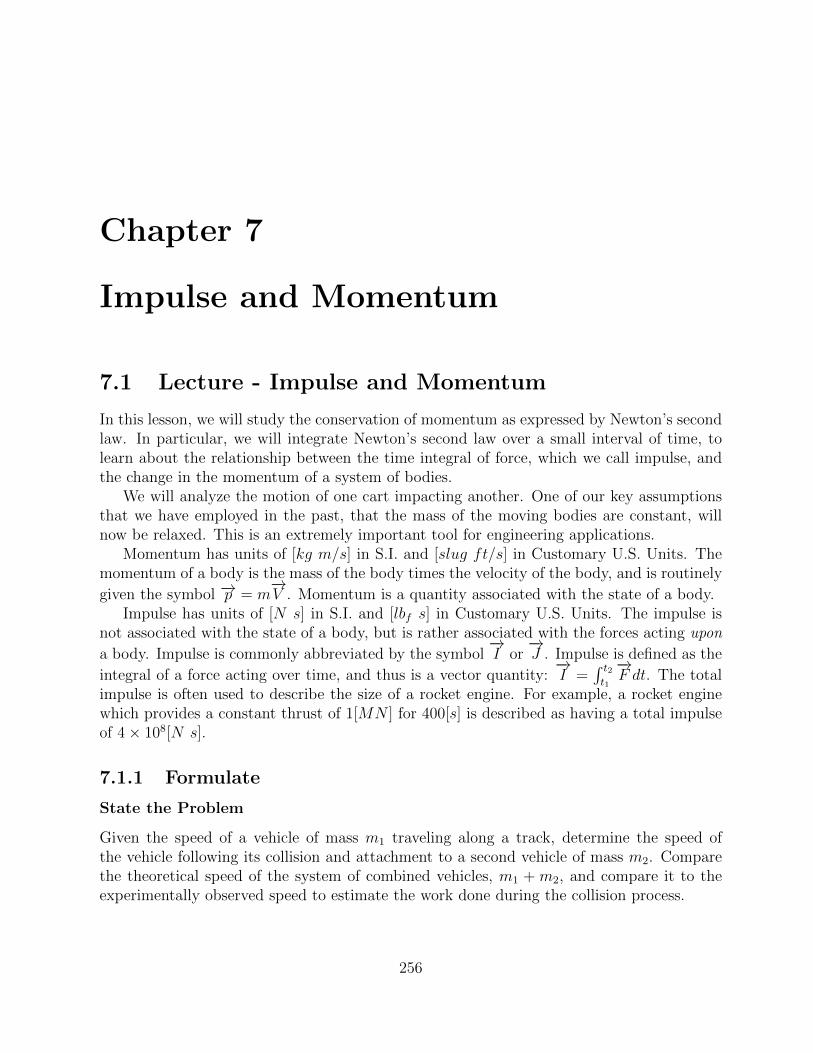
Chapter 7
Impulse and Momentum
7.1 Lecture - Impulse and Momentum
In this lesson, we will study the conservation of momentum as expressed by Newton’s secondlaw. In particular, we will integrate Newton’s second law over a small interval of time, tolearn about the relationship between the time integral of force, which we call impulse, andthe change in the momentum of a system of bodies.
We will analyze the motion of one cart impacting another. One of our key assumptionsthat we have employed in the past, that the mass of the moving bodies are constant, willnow be relaxed. This is an extremely important tool for engineering applications.
Momentum has units of [kg m/s] in S.I. and [slug ft/s] in Customary U.S. Units. Themomentum of a body is the mass of the body times the velocity of the body, and is routinelygiven the symbol �!p = m
�!V . Momentum is a quantity associated with the state of a body.
Impulse has units of [N s] in S.I. and [lbf s] in Customary U.S. Units. The impulse isnot associated with the state of a body, but is rather associated with the forces acting upona body. Impulse is commonly abbreviated by the symbol
�!I or
�!J . Impulse is defined as the
integral of a force acting over time, and thus is a vector quantity:�!I =
R t2
t1
�!F dt. The total
impulse is often used to describe the size of a rocket engine. For example, a rocket enginewhich provides a constant thrust of 1[MN ] for 400[s] is described as having a total impulseof 4⇥ 108[N s].
7.1.1 Formulate
State the Problem
Given the speed of a vehicle of mass m1
traveling along a track, determine the speed ofthe vehicle following its collision and attachment to a second vehicle of mass m
2
. Comparethe theoretical speed of the system of combined vehicles, m
1
+ m2
, and compare it to theexperimentally observed speed to estimate the work done during the collision process.
256
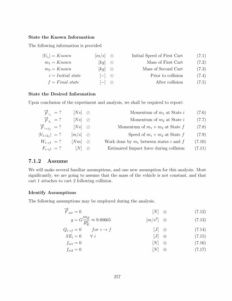
State the Known Information
The following information is provided
|V1i | = Known [m/s] � Initial Speed of First Cart (7.1)
m1
= Known [kg] � Mass of First Cart (7.2)
m2
= Known [kg] � Mass of Second Cart (7.3)
i = Initial state [�] � Prior to collision (7.4)
f = Final state [�] � After collision (7.5)
State the Desired Information
Upon conclusion of the experiment and analysis, we shall be required to report:
�!p1i
= ? [Ns] ↵ Momentum of m1
at State i (7.6)�!p
2i= ? [Ns] ↵ Momentum of m
2
at State i (7.7)�!p
1+2f= ? [Ns] ↵ Momentum of m
1
+m2
at State f (7.8)
|V1+2f
| = ? [m/s] ↵ Speed of m1
+m2
at State f (7.9)
Wi!f = ? [Nm] ↵ Work done by m1
between states i and f (7.10)
Fi!f = ? [N ] ↵ Estimated Impact force during collision (7.11)
7.1.2 Assume
We will make several familiar assumptions, and one new assumption for this analysis. Mostsignificantly, we are going to assume that the mass of the vehicle is not constant, and thatcart 1 attaches to cart 2 following collision.
Identify Assumptions
The following assumptions may be employed during the analysis.
�!F air = 0 [N ] � (7.12)
g = GmE
R2
E
⇡ 9.80665 [m/s2] � (7.13)
Qi!f = 0 for i ! f [J ] � (7.14)
SEi = 0 8 i [J ] � (7.15)
fm1
= 0 [N ] � (7.16)
fm2
= 0 [N ] � (7.17)
257
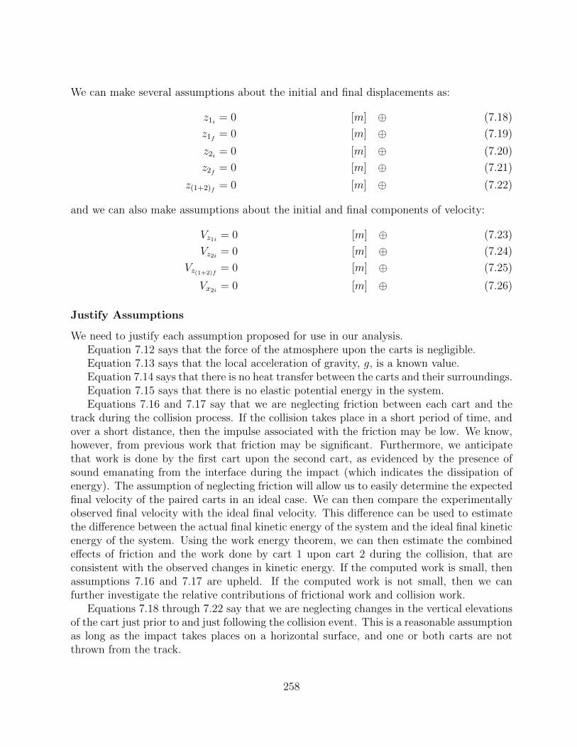
We can make several assumptions about the initial and final displacements as:
z1i = 0 [m] � (7.18)
z1f
= 0 [m] � (7.19)
z2i = 0 [m] � (7.20)
z2f
= 0 [m] � (7.21)
z(1+2)f
= 0 [m] � (7.22)
and we can also make assumptions about the initial and final components of velocity:
Vz1i = 0 [m] � (7.23)
Vz2i = 0 [m] � (7.24)
Vz(1+2)f
= 0 [m] � (7.25)
Vx2i = 0 [m] � (7.26)
Justify Assumptions
We need to justify each assumption proposed for use in our analysis.Equation 7.12 says that the force of the atmosphere upon the carts is negligible.Equation 7.13 says that the local acceleration of gravity, g, is a known value.Equation 7.14 says that there is no heat transfer between the carts and their surroundings.Equation 7.15 says that there is no elastic potential energy in the system.Equations 7.16 and 7.17 say that we are neglecting friction between each cart and the
track during the collision process. If the collision takes place in a short period of time, andover a short distance, then the impulse associated with the friction may be low. We know,however, from previous work that friction may be significant. Furthermore, we anticipatethat work is done by the first cart upon the second cart, as evidenced by the presence ofsound emanating from the interface during the impact (which indicates the dissipation ofenergy). The assumption of neglecting friction will allow us to easily determine the expectedfinal velocity of the paired carts in an ideal case. We can then compare the experimentallyobserved final velocity with the ideal final velocity. This di↵erence can be used to estimatethe di↵erence between the actual final kinetic energy of the system and the ideal final kineticenergy of the system. Using the work energy theorem, we can then estimate the combinede↵ects of friction and the work done by cart 1 upon cart 2 during the collision, that areconsistent with the observed changes in kinetic energy. If the computed work is small, thenassumptions 7.16 and 7.17 are upheld. If the computed work is not small, then we canfurther investigate the relative contributions of frictional work and collision work.
Equations 7.18 through 7.22 say that we are neglecting changes in the vertical elevationsof the cart just prior to and just following the collision event. This is a reasonable assumptionas long as the impact takes places on a horizontal surface, and one or both carts are notthrown from the track.
258
Equations 7.23 through 7.25 state the the vertical component of velocity of both cartsremains zero throughout the collision process. This is also a reasonable assumption as longas the impact takes places on a horizontal surface, and one or both carts are not thrownfrom the track.
Equation 7.26 states further that the second cart is at rest, and also has no horizontalcomponent of velocity just prior to the collision. This is a reasonable assumption for theproblem as we have defined it.
7.1.3 Chart
Schematic Diagrams
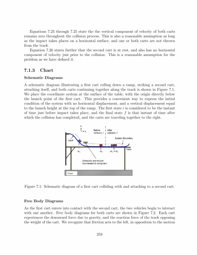
A schematic diagram illustrating a first cart rolling down a ramp, striking a second cart,attaching itself, and both carts continuing together along the track is shown in Figure 7.1.We place the coordinate system at the surface of the table, with the origin directly belowthe launch point of the first cart. This provides a convenient way to express the initialcondition of the system with no horizontal displacement, and a vertical displacement equalto the launch height at the top of the ramp. The first state i is considered to be the instantof time just before impact takes place, and the final state f is that instant of time afterwhich the collision has completed, and the carts are traveling together to the right.
Figure 7.1: Schematic diagram of a first cart colliding with and attaching to a second cart.
Free Body Diagrams
As the first cart enters into contact with the second cart, the two vehicles begin to interactwith one another. Free body diagrams for both carts are shown in Figure 7.2. Each cartexperiences the downward force due to gravity, and the reaction force of the track opposingthe weight of the cart. We recognize that friction acts to the left, in opposition to the motion
259
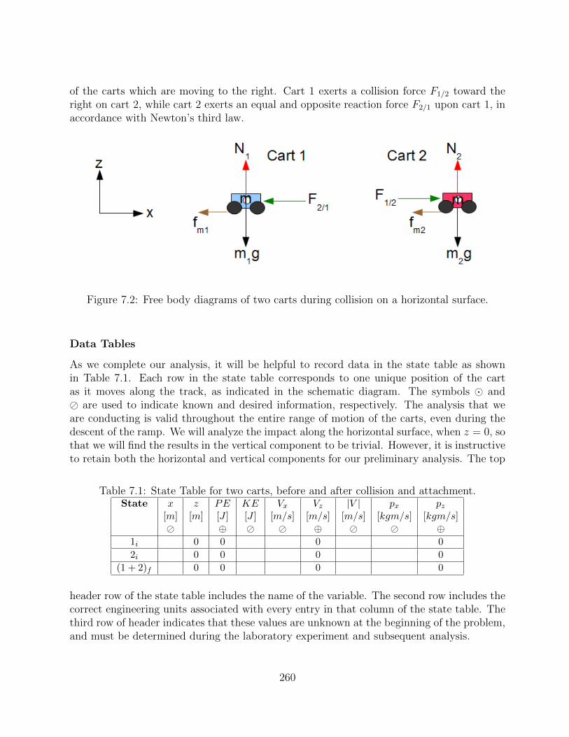
of the carts which are moving to the right. Cart 1 exerts a collision force F1/2 toward the
right on cart 2, while cart 2 exerts an equal and opposite reaction force F2/1 upon cart 1, in
accordance with Newton’s third law.
Figure 7.2: Free body diagrams of two carts during collision on a horizontal surface.
Data Tables
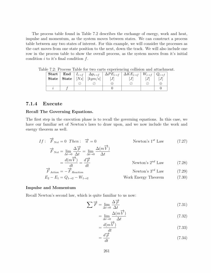
As we complete our analysis, it will be helpful to record data in the state table as shownin Table 7.1. Each row in the state table corresponds to one unique position of the cartas it moves along the track, as indicated in the schematic diagram. The symbols � and↵ are used to indicate known and desired information, respectively. The analysis that weare conducting is valid throughout the entire range of motion of the carts, even during thedescent of the ramp. We will analyze the impact along the horizontal surface, when z = 0, sothat we will find the results in the vertical component to be trivial. However, it is instructiveto retain both the horizontal and vertical components for our preliminary analysis. The top
Table 7.1: State Table for two carts, before and after collision and attachment.State x z PE KE Vx Vz |V | px pz
[m] [m] [J ] [J ] [m/s] [m/s] [m/s] [kgm/s] [kgm/s]↵ � ↵ ↵ � ↵ ↵ �
1i 0 0 0 02i 0 0 0 0
(1 + 2)f 0 0 0 0
header row of the state table includes the name of the variable. The second row includes thecorrect engineering units associated with every entry in that column of the state table. Thethird row of header indicates that these values are unknown at the beginning of the problem,and must be determined during the laboratory experiment and subsequent analysis.
260
The process table found in Table 7.2 describes the exchange of energy, work and heat,impulse and momentum, as the system moves between states. We can construct a processtable between any two states of interest. For this example, we will consider the processes asthe cart moves from one state position to the next, down the track. We will also include onerow in the process table to show the overall process, as the system moves from it’s initialcondition i to it’s final condition f .
Table 7.2: Process Table for two carts experiencing collision and attachment.Start End Ii!f �pi!f �PEi!f �KEi!f Wi!f Qi!f
State State [Ns] [kgm/s] [J ] [J ] [J ] [J ]↵ ↵ � ↵ ↵ �
i f 0 0
7.1.4 Execute
Recall The Governing Equations.
The first step in the execution phase is to recall the governing equations. In this case, wehave our familiar set of Newton’s laws to draw upon, and we now include the work andenergy theorem as well.
If :�!F Net = 0 Then : �!a = 0 Newton’s 1st Law (7.27)
�!F Net = lim
�t!0
��!p�t
= lim�t!0
�(m�!V )
�t
=d(m
�!V )
dt=
d�!pdt
Newton’s 2nd Law (7.28)
�!F Action = ��!
F Reaction Newton’s 3rd Law (7.29)
E2
� E1
= Q1!2
�W1!2
Work Energy Theorem (7.30)
Impulse and Momentum
Recall Newton’s second law, which is quite familiar to us now:X�!
F = lim�t!0
��!p�t
(7.31)
= lim�t!0
�(m�!V )
�t(7.32)
=d(m
�!V )
dt(7.33)
=d�!pdt
(7.34)
261
The last version, Equation 7.34, is the form of Newton’s second law that we will focus onthis week. This law says that “The net external force acting upon a body is equal to thetime rate of change of the linear momentum of the body.” Let’s rearrange Equation 7.34by separating the di↵erentials, and integrating the result between some initial time, ti andsome final time, tf :
X�!F dt = d�!p (7.35)
Z tf
ti
X�!F dt =
Z f
i
d�!p (7.36)
The impulse is defined as the integral of force over time. We evaluate the result between theupper and lower limits as:
�!I |tfti = �!p |fi (7.37)
�!I f �
�!I i =
�!p f ��!p i (7.38)
��!I i!f = ��!p i!f (7.39)
[N ][s] = [kgm/s] Derived Units
[kgm/s2][s] = [kgm/s] Basic Units
where we have defined a new term called the “impulse”,�!I , as the integral of a force acting
over some interval of time, in analogy to the way we defined “work” as force acting over somedisplacement. Equation 7.39 tells us many useful things. Most significantly, the impulseand momentum form of Newton’s second law did not require us to make any assumptionsabout the mass of the system being constant. Previously, we had to assume that the masswas constant, so that m could be taken outside of the derivative or integral operator. Thisgeneralization will be particularly helpful in classes of problems where in two bodies combine(such as collisions), where two bodies separate (such as the separation of a rocket stage), orwhen the mass of the body is not constant (such as the consumption of fuel contributing toa significant change in the mass of the vehicle, like an aircraft with wing tanks full of fuel).
This generalized version of Newton’s second law allow us to predict motion of a systemof interacting bodies. Let’s use the impulse and momentum formula to analyze a problemthat we would have found to be intractable previously.
Simplify the Governing Equations.
Let’s rearrange Equation 7.28 by separating the di↵erentials, and integrating only the righthand side of the equation, while leaving the left hand side of the equation in the original
262
integral form:X�!
F dt = d�!p (7.40)Z tf
ti
X�!F dt =
Z f
i
d�!p (7.41)
Z tf
ti
X�!F dt = �!p |fi = �!p f ��!p i (7.42)
[N ][s] = [kgm/s] Derived Units
[kgm/s2][s] = [kgm/s] Basic Units
From the free body diagram shown in Figure 7.2, (and Newton’s third law, Equation 7.29)we know that the action and reaction forces between the two carts are equal and opposite.By virtue of assumptions 7.18 through 7.25, we can say that the upward normal force exertedby the track upon each cart is equal to the downward force exerted due to the gravitationalaction of the Earth. Assumptions 7.16 and 7.17 state that we can neglect friction during thecollision process. Thus, in light of all these assumptions, Equation 7.42 reduces to
!0z }| {Z f
i
X�!F dt = �!p f ��!p i = 0 (7.43)
[kgm/s2][s] = [kgm/s] Basic Units
Inventory the Governing Equations, Known, and Desired Information.
Using the definition of momentum, we can state:
px1i = m
1
Vx1i ↵ (7.44)
pz1i = m
1
Vz1i = 0 � (7.45)
px2i = m
2
Vx2i = 0 � (7.46)
pz2i = m
2
Vz2i = 0 � (7.47)
px(1+2)f
= (m1
+m2
)Vx(1+2)f
↵ (7.48)
pz(1+2)f
= (m1
+m2
)Vz(1+2)f
= 0 � (7.49)
These equations are su�cient for us to fill in many entries in the state table. Let us substituteEquations 7.44 through 7.49 into Equation 7.43 and algebraically simplify the result to get:
0 = (m1
+m2
)Vx(1+2)f
�m1
Vx1i (7.50)
Solve
Equation 7.50 contains two unknowns. Without additional information, we cannot com-pletely solve the problem. However, if we can determine the speed of cart 1 just prior to
263
the collision, then we can symbolically find the speed of the two attached carts following thecollision as
Vx(1+2)f
=m
1
(m1
+m2
)Vx
1i (7.51)
[m/s] =[kg]
[kg][m/s] Units Validation
[↵] =[�]
[�][↵] Inventory
If the collision between the two carts is ideal (and does not dissipate any energy) then weexpect Equation 7.51 to predict the velocity of the two carts leaving the collision site. Usingthe tools we have learned about in previous labs, we should be able to measure the speed ofcart 1 prior to impact as well as the speed of the combined carts following impact. Usingthese observed values in Equation 7.51 will allow us to assess the validity of our assumptionsregarding friction and the energy loss during impact.
7.1.5 Test
Validate
Another way to predict the motion of the carts before, during, and after the collision is tocombine our analysis of work and energy from last week with our analysis of impulse andmomentum from this week. As an exercise in preparation for your recitation, please usethe work energy theorem and knowledge of the vertical displacement of cart 1 at the top ofthe ramp to predict the speed of cart 1 prior to impact, and then use 7.51 to predict thespeed following the collision. Analyze this same collision problem in your logbook, usingthe principle of the conservation of energy. Be prepared to discuss the significance of youranalysis.
Verify
We have verified that the units on each result are correct. As further verification, pleasecompute the sum of the kinetic energy and gravitational potential energy for cart 1 and 2just prior to and just following the collision event. How does the total energy of the systemcompare?
Apply Intuition
The results are consistent with our intuition. We expect that a light-weight fast movingcart will collide with the second cart, and that the two carts, heavier in weight, will moveforward at reduced speed. Are your theoretical equations consistent with your expectationof the phenomena based on personal experience?
264
Report
By following the well-defined problem solving process, and creating documentation through-out, all information needed for a formal report is readily available.
7.1.6 Iterate
In lab, we will conduct multiple trials of this experiment. Each student member of the labgroup should conduct an independent trial, and analyze a unique data set. Each studentshould select a di↵erent launching height for cart 1, which will introduce a variable initialvelocity of the cart prior to the collision.
265
7.2 Lab - Two Body Impact
7.2.1 Scope
This week in lab we will use the ultrasonic transducer to record the one-dimensional motion ofa cart that passes beneath the transducer and then impacts a second, stationary cart fartherdown the track. The carts are designed to attach to one another following the collision andwill roll away from the collision site in tandem. Each member of the lab team will conducta separate trial, and obtain a unique sensor recording for their personal analysis. We willuse the ultrasonic transducer to record the horizontal motion of the carts during the event.Note that a digital imaging system could also be used, particularly if we were concerned withmotion in two dimensions. After capturing their voltage vs. time data set, each student willprocess the data to estimate the mean speed of the carts prior to and following the collision.
7.2.2 Goal
The goals of this laboratory experiment are to
1. demonstrate the principle of conservation of momentum,
2. demonstrate the concepts of impulse and momentum, derived from Newton’s secondlaw, and
3. expand our ability to analyze multi-body systems experiencing impact.
7.2.3 Units of Measurement to Use
All reports shall be presented in the SI system of units. Raw data may be collected in avariety of units.
Quantity Basic units Derived units
Length [m] [m]Mass [kg] [kg]Time [s] [s]
Velocity [m/s] [m/s]Force [kgm/s
2] [N ]Energy [kgm2
/s
2] [J ] or [N ][m]Impulse [kgm/s] [N ][s]
Momentum [kgm/s] [N ][s]
Table 7.3: Units of Measurement to be used for two body impact.
266
7.2.4 Measurement Uncertainty
The uncertainty relationships discussed here and in each Measurement Uncertainty sectionof this text are summarized for your convenience in the Engineering Mechanics ReferenceTable, which is posted on myCourses. These uncertainty relationships can be applied to theenergy, work, distance traveled and friction coe�cient calculations and force calculations tohelp quantify the range of uncertainty in your analysis.
✏x = ±ILC/2 Position Uncertainty (7.52)
✏V = ✏x/�t Instantaneous Speed Uncertainty (7.53)
✏V =✏V
2pNa
Central Di↵erence Mean Speed Uncertainty (7.54)
(7.55)
Please complete the following task in your logbook.
Derive equations for uncertainties for the items listed below that will be calculated inStudio. Keep in mind that the uncertainty associated with the masses of the carts is verysmall compared with other variables in these equations. Therefore, the mass terms can betreated as constants when deriving the uncertainty equations. Refer to the similar analysisthat was done in the week 6 Studio.
• Momentum
• Kinetic Energy
• Work Done during Impact
• Estimated Impact force
7.2.5 Reference Documents
The following documents may be helpful; user’s guide for the computer, user’s guide for dataacquisition software, user’s guide for the camera.
7.2.6 Terminology
The following terms must be fully understood in order to achieve the educational objectivesof this laboratory experiment.
Force Displacement MomentumVelocity Speed AccelerationEnergy Work ImpulseGravitational Potential Energy Kinetic Energy
267
7.2.7 Summary of Test Method
A video of the lab experiment is available for viewing on myCourses. This video will provideyou with an understanding of what you need to do during the lab. Please review this videobefore reading on, since it will provide you a nice overview of the experiment and allow youto better understand the following information.
7.2.8 Calibration and Standardization
The Lead Technologist and Assistant Technologist shall conduct a careful calibration of theultrasonic transducer using a calibration configuration that reflects the actual experimentalsetup for the trials. Confirm that the transducer data collection software is functioningproperly by acquiring a set of voltage vs. time as the carts move along the track.
7.2.9 Apparatus
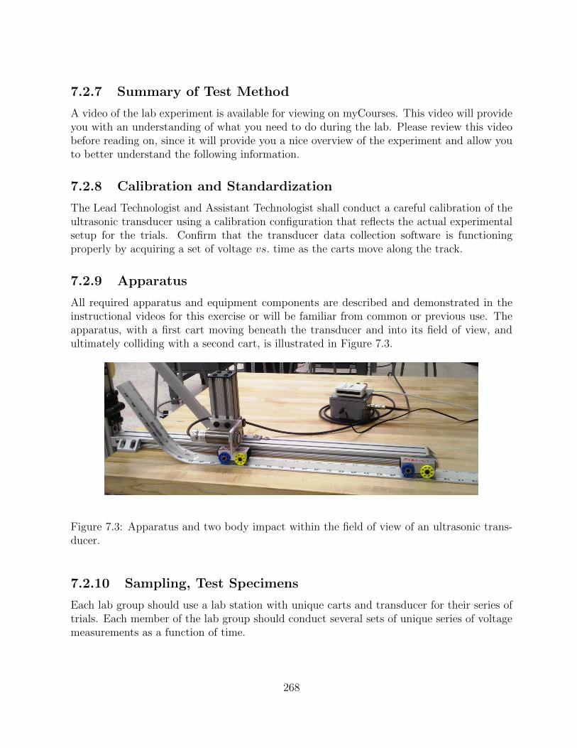
All required apparatus and equipment components are described and demonstrated in theinstructional videos for this exercise or will be familiar from common or previous use. Theapparatus, with a first cart moving beneath the transducer and into its field of view, andultimately colliding with a second cart, is illustrated in Figure 7.3.
Figure 7.3: Apparatus and two body impact within the field of view of an ultrasonic trans-ducer.
7.2.10 Sampling, Test Specimens
Each lab group should use a lab station with unique carts and transducer for their series oftrials. Each member of the lab group should conduct several sets of unique series of voltagemeasurements as a function of time.
268
7.2.11 Preparation of Apparatus
All required equipment for conducting the laboratory exercise is made available either withinone or both of the drawers attached to the lab bench or from the laboratory instructor. Youare expected to bring all other necessary materials, particularly your logbook and a flashdrive for storing electronic data as appropriate. You are to follow the general specificationsfor team roles within the lab. Although there are specific, individual expectations for eachrole, you are each responsible overall to ensure that the objectives and requirements of thelaboratory exercise are met, and that all rules and procedures are followed at all times,especially any that are related to safety in the lab. When finished, all equipment is to bereturned to the proper location, in proper working order.
7.2.12 Procedure - Lab Portion
The instructional videos for this exercise cover the specific procedures to follow as you setup the apparatus to make measurements, and for actually collecting data with the variousdevices and software interfaces. More generally, you should always observe the followinggeneral procedures as you conduct any of the exercises in this laboratory.
1. Come prepared to lab, having watched the videos in detail, then completing the asso-ciated lab quiz and preparing your logbook before you arrive to class.
2. Follow the basic outline of elements to include in your logbook related to headers,footer, and signatures.
3. As you conduct the exercise, please pay attention to the following safety concerns:
• Watch for tripping hazards, due to cables and moving elements.
• Watch for pinch points, during assembling and disassembly.
• Be careful of shock hazards while connecting and operating electrical components
4. Every week, for every exercise, your logbook will minimally contain background notesand information that you collect before the lab, at least one schematic of the apparatus,various standard tables for recording the organization of your roles and equipmentused, the actual data collected and/or notes related to the data collected (if doneelectronically for instance), and any other information relevant to the reporting andanalysis of the data and understanding of the exercise itself.
5. All students should create and complete a table indicating the sta�ng plan for theweek (that is, the roles assumed by each group member), as shown in Table 1.2.
6. All students should create and complete a table listing all equipment used for the exer-cise, the location (from where was it obtained: top drawer, bottom drawer, instructor?)and all identifying information that is readily available. If the manufacturer and se-rial number are available, then record both (this would be an ideal scenario). If not,
269
record whatever you can about the component. In some, cases, there will be no specificidentifying information whatsoever either because of the simplicity of the component,or because of its origin. In these cases, just identify the component as best you can,perhaps as “Manufactured by RITME.” The point here is to give as much informationas possible in case someone was to try to reproduce or verify what you did. Refer toTable 1.3.
7. For the Lab Manager only: create a key sign-out/sign-in table for obtaining thekey to the equipment drawers, as shown in Table 1.4.
8. All students should create a table or series of tables as appropriate to collect his/herown data for the exercise, as well as any specific notes related to the data collectionactivities. In those cases where data collection is done electronically, there may not beany data tables required.
9. Many of the laboratory exercises will require the use of a specific software interfacefor measurements and/or control. In all cases, these will be made available on themyCourses site unless stated otherwise.
10. The Scribe (or a designated alternative) should take a photo of each group memberperforming some aspect of the laboratory exercise for inclusion in the lab reportthat will be generated during the studio session. Refer to the example lab report formore details.
11. Record all relevant data and observations in your logbook, even those that may nothave been explicitly requested or indicated by the textbook or videos. If in doubtabout any measurements, it is better to make the measurement rather than not.
12. When you are finished with all lab activities, make sure that all equipment has beenreturned to the proper place. Log out of the computer, and straighten up everythingon the lab bench as you found it. Put the lab stools back under the bench and out ofthe way.
13. Prepare for the upcoming studio session for the week by carefully read and understandSection 4.3 of the textbook, and complete the Studio pre-work prior to your arrival atStudio.
270
7.3 Studio - Conservation of Linear Momentum
The theory needed to analysis the data is discussed in Section 7.1 of the text. Section 7.3.1Calculation and Interpretation of Results provides a summary of equations that you willneed to complete the Studio. Section 7.2.4 Measurement Uncertainty, describes the processfor analyzing the experimental errors. There will be uncertainty equation derivations thatyou need to complete prior to arriving at studio and these are listed in the MeasurementUncertainty section.
Record all observations and notes about your studio procedures inyour logbook.
7.3.1 Calculation and Interpretation of Results
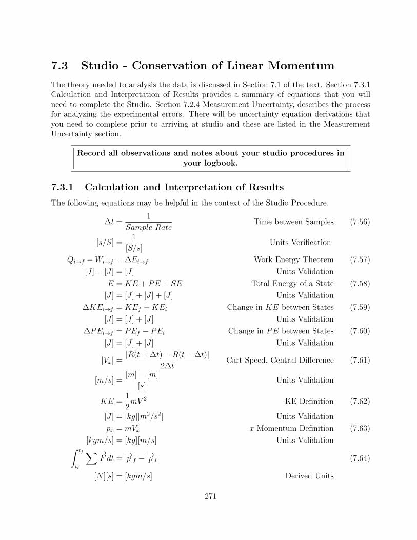
The following equations may be helpful in the context of the Studio Procedure.
�t =1
Sample RateTime between Samples (7.56)
[s/S] =1
[S/s]Units Verification
Qi!f �Wi!f = �Ei!f Work Energy Theorem (7.57)
[J ]� [J ] = [J ] Units Validation
E = KE + PE + SE Total Energy of a State (7.58)
[J ] = [J ] + [J ] + [J ] Units Validation
�KEi!f = KEf �KEi Change in KE between States (7.59)
[J ] = [J ] + [J ] Units Validation
�PEi!f = PEf � PEi Change in PE between States (7.60)
[J ] = [J ] + [J ] Units Validation
|Vx| =|R(t+�t)�R(t��t)|
2�tCart Speed, Central Di↵erence (7.61)
[m/s] =[m]� [m]
[s]Units Validation
KE =1
2mV 2 KE Definition (7.62)
[J ] = [kg][m2/s2] Units Validation
px = mVx x Momentum Definition (7.63)
[kgm/s] = [kg][m/s] Units ValidationZ tf
ti
X�!F dt = �!p f ��!p i (7.64)
[N ][s] = [kgm/s] Derived Units
271
7.3.2 Procedure - Studio Portion
Studio Pre-work
Prior to arriving at Studio, each student should have acquired the necessary data in lab,recorded data in your notebook and stored data on a thumb drive. You should also have acorresponding schematic that clearly identifies where each measurement was made in sym-bolic notation.
In addition, each you will complete several steps of the Studio exercise. This will allowmore quality time with the instructor to discuss the physical meaning of the analysis results.You will upload your studio pre-work to your individual drop-box for the correspondingweek. You will receive a quiz grade based on the completeness of your submission.
Please complete at least steps 1-5 and upload your pre-work spreadsheet toyour individual drop-box, before coming to coming to Studio. You can work on theremaining portions of the exercise during Studio. All steps with the exception of the reportare due within 24 hrs after leaving Studio.
Videos
There are videos available to help with some of the excel techniques that may be new to you.We have highlighted steps where videos might be helpful. However, you can also completethe steps simply by following the written instructions. For those procedures that do nothave videos, you should rely on previously developed skills. You may want to review videosfrom previous weeks if you feel that you need a refresher on some of the techniques.
Steps to Complete the Analysis
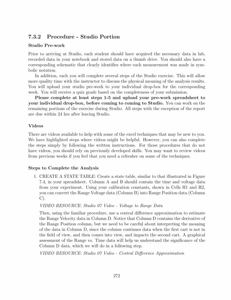
1. CREATE A STATE TABLE: Create a state table, similar to that illustrated in Figure7.4, in your spreadsheet. Column A and B should contain the time and voltage datafrom your experiment. Using your calibration constants, shown in Cells H1 and H2,you can convert the Range Voltage data (Column B) into Range Position data (ColumnC).
VIDEO RESOURCE: Studio 07 Video - Voltage to Range Data
Then, using the familiar procedure, use a central di↵erence approximation to estimatethe Range Velocity data in Column D. Notice that Column D contains the derivative ofthe Range Position column, but we need to be careful about interpreting the meaningof the data in Column D, since the column continues data when the first cart is not inthe field of view, and then comes into view, and impacts the second cart. A graphicalassessment of the Range vs. Time data will help us understand the significance of theColumn D data, which we will do in a following step.
VIDEO RESOURCE: Studio 07 Video - Central Di↵erence Approximation
272
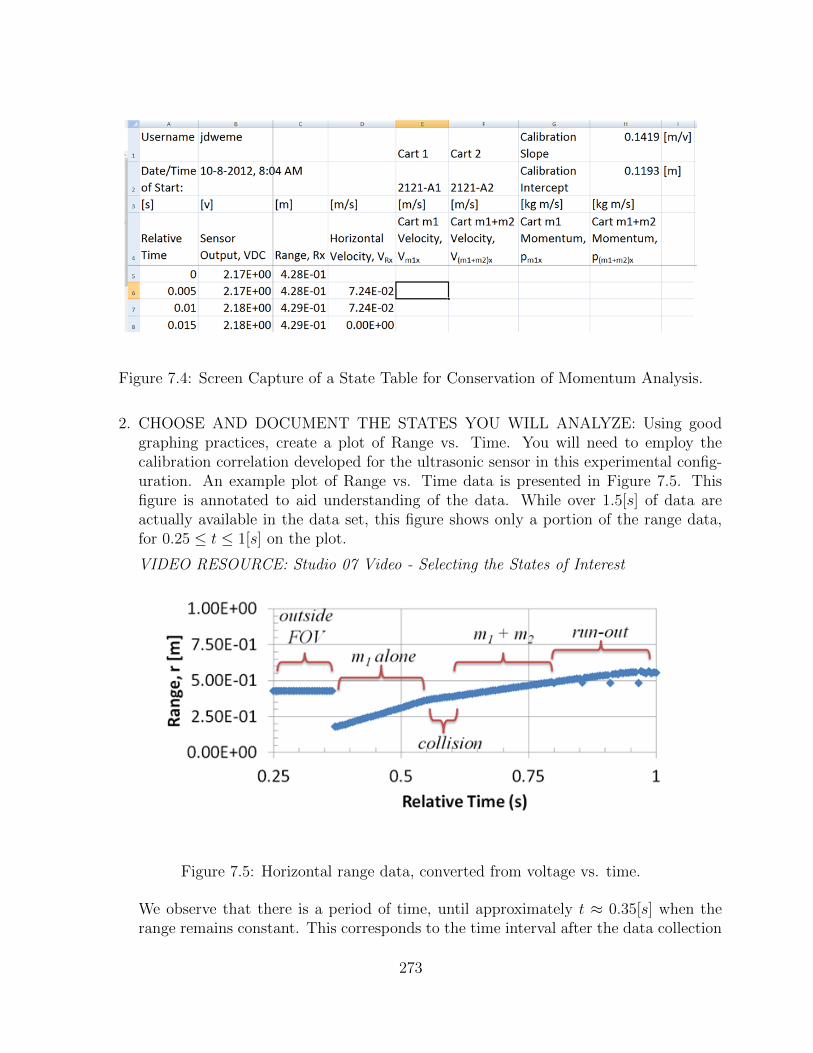
Figure 7.4: Screen Capture of a State Table for Conservation of Momentum Analysis.
2. CHOOSE AND DOCUMENT THE STATES YOU WILL ANALYZE: Using goodgraphing practices, create a plot of Range vs. Time. You will need to employ thecalibration correlation developed for the ultrasonic sensor in this experimental config-uration. An example plot of Range vs. Time data is presented in Figure 7.5. Thisfigure is annotated to aid understanding of the data. While over 1.5[s] of data areactually available in the data set, this figure shows only a portion of the range data,for 0.25 t 1[s] on the plot.
VIDEO RESOURCE: Studio 07 Video - Selecting the States of Interest
Figure 7.5: Horizontal range data, converted from voltage vs. time.
We observe that there is a period of time, until approximately t ⇡ 0.35[s] when therange remains constant. This corresponds to the time interval after the data collection
273
program has been started, until the first cart descends the incline, passes beneath thetransducer, and finally enters into the field of view. Then, as the first cart entersthe field of view of the transducer, the range increases approximately linearly in time,over the time interval 0.35 t 0.6[s]. The observation that the range increaseslinearly with time is characteristic of low friction motion of the cart along the track.Eventually, the first cart collides with the second cart, and becomes attached to thesecond cart by virtue of the hook-and-loop fasteners. The collision happens during theinterval 0.6 t 0.65[s]. After the collision is complete, t � 0.65[s], the two cartsmove together, with a linearly increasing range, also indicative of a nearly constantvelocity. As the combined carts move farther to the right, they begin to slow down asa result of the cumulative friction. As they get farther from the transducer surface,the noise in the data increases.
Create a plot of Range vs. Time, print this plot out, paste it in your logbook, andannotate it by hand, similarly to the figure shown. Identify the interval of time thatyou will consider to be that of m
1
moving alone, and a similar length time period thatyou will consider to be that of m
1
+m2
moving in tandem. Write these time incrementsin your logbook, using a table like the one shown in Figure 7.5.
Table 7.4: Identification of States of Interest.States Start time End time First Row Last Row
[s] [s] [�] [�]m
1
Alonem
1
+m
2
in Tandem
After identifying the start and stop time, look at your spreadsheet, and determine thecorresponding first and last rows of data that are relevant to each time interval.
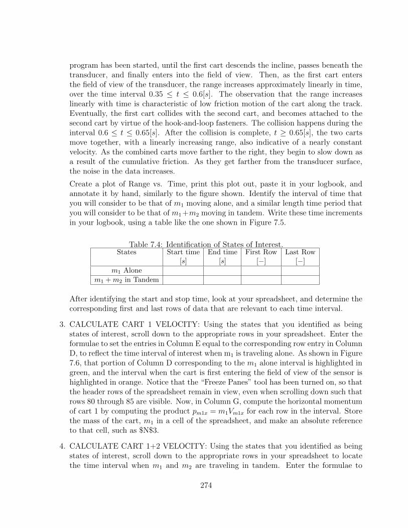
3. CALCULATE CART 1 VELOCITY: Using the states that you identified as beingstates of interest, scroll down to the appropriate rows in your spreadsheet. Enter theformulae to set the entries in Column E equal to the corresponding row entry in ColumnD, to reflect the time interval of interest when m
1
is traveling alone. As shown in Figure7.6, that portion of Column D corresponding to the m
1
alone interval is highlighted ingreen, and the interval when the cart is first entering the field of view of the sensor ishighlighted in orange. Notice that the “Freeze Panes” tool has been turned on, so thatthe header rows of the spreadsheet remain in view, even when scrolling down such thatrows 80 through 85 are visible. Now, in Column G, compute the horizontal momentumof cart 1 by computing the product pm1x = m
1
Vm1x for each row in the interval. Storethe mass of the cart, m
1
in a cell of the spreadsheet, and make an absolute referenceto that cell, such as $N$3.
4. CALCULATE CART 1+2 VELOCITY: Using the states that you identified as beingstates of interest, scroll down to the appropriate rows in your spreadsheet to locatethe time interval when m
1
and m2
are traveling in tandem. Enter the formulae to
274
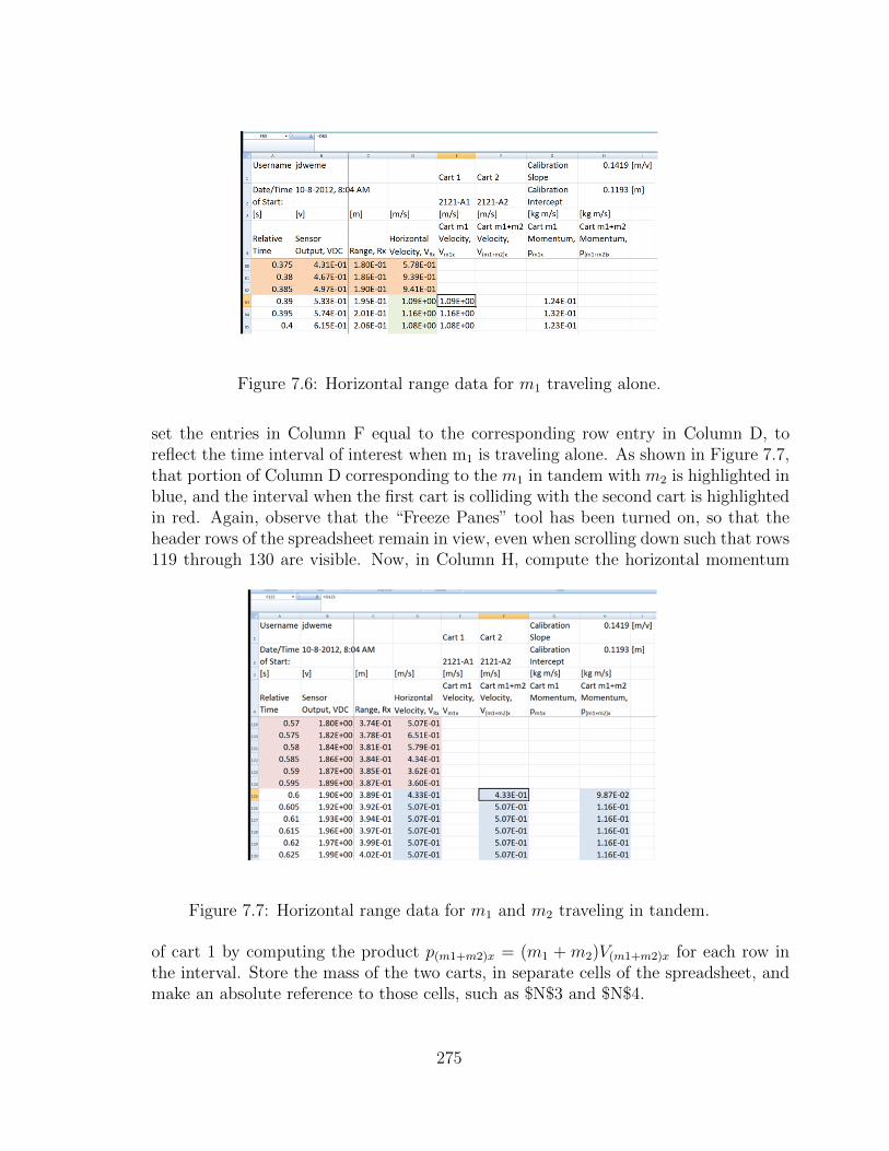
Figure 7.6: Horizontal range data for m1
traveling alone.
set the entries in Column F equal to the corresponding row entry in Column D, toreflect the time interval of interest when m
1
is traveling alone. As shown in Figure 7.7,that portion of Column D corresponding to the m
1
in tandem with m2
is highlighted inblue, and the interval when the first cart is colliding with the second cart is highlightedin red. Again, observe that the “Freeze Panes” tool has been turned on, so that theheader rows of the spreadsheet remain in view, even when scrolling down such that rows119 through 130 are visible. Now, in Column H, compute the horizontal momentum
Figure 7.7: Horizontal range data for m1
and m2
traveling in tandem.
of cart 1 by computing the product p(m1+m2)x = (m
1
+m2
)V(m1+m2)x for each row in
the interval. Store the mass of the two carts, in separate cells of the spreadsheet, andmake an absolute reference to those cells, such as $N$3 and $N$4.
275
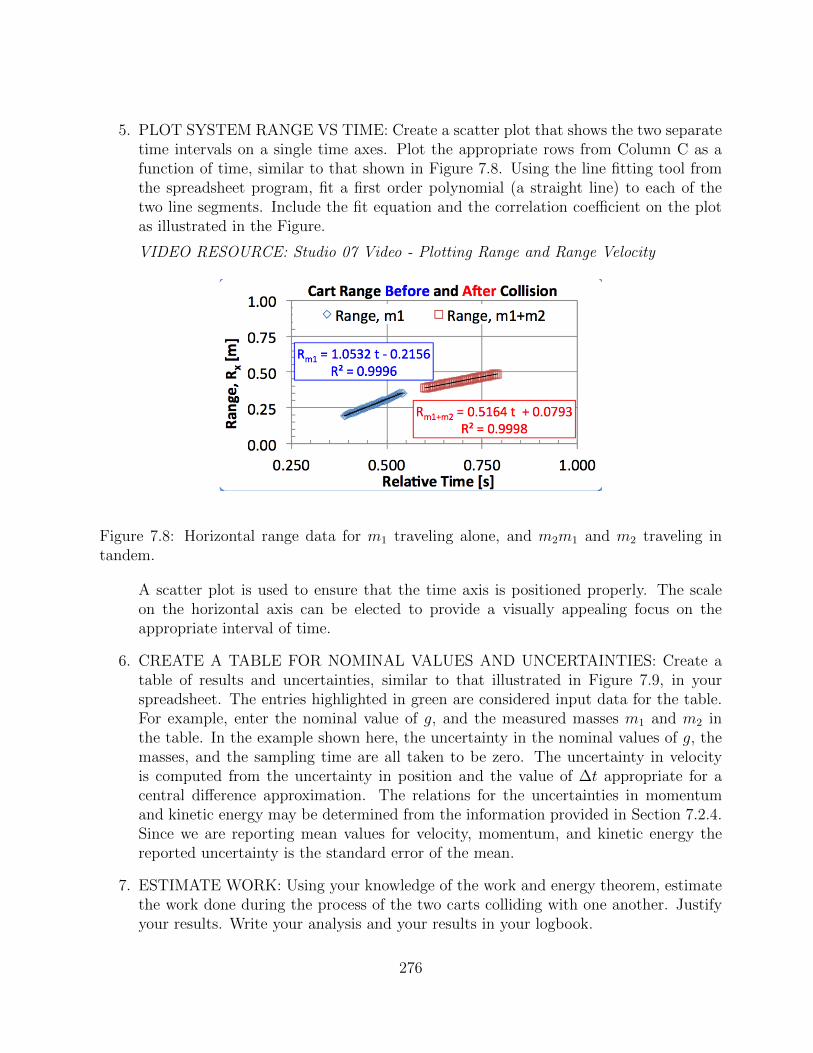
5. PLOT SYSTEM RANGE VS TIME: Create a scatter plot that shows the two separatetime intervals on a single time axes. Plot the appropriate rows from Column C as afunction of time, similar to that shown in Figure 7.8. Using the line fitting tool fromthe spreadsheet program, fit a first order polynomial (a straight line) to each of thetwo line segments. Include the fit equation and the correlation coe�cient on the plotas illustrated in the Figure.
VIDEO RESOURCE: Studio 07 Video - Plotting Range and Range Velocity
Figure 7.8: Horizontal range data for m1
traveling alone, and m2
m1
and m2
traveling intandem.
A scatter plot is used to ensure that the time axis is positioned properly. The scaleon the horizontal axis can be elected to provide a visually appealing focus on theappropriate interval of time.
6. CREATE A TABLE FOR NOMINAL VALUES AND UNCERTAINTIES: Create atable of results and uncertainties, similar to that illustrated in Figure 7.9, in yourspreadsheet. The entries highlighted in green are considered input data for the table.For example, enter the nominal value of g, and the measured masses m
1
and m2
inthe table. In the example shown here, the uncertainty in the nominal values of g, themasses, and the sampling time are all taken to be zero. The uncertainty in velocityis computed from the uncertainty in position and the value of �t appropriate for acentral di↵erence approximation. The relations for the uncertainties in momentumand kinetic energy may be determined from the information provided in Section 7.2.4.Since we are reporting mean values for velocity, momentum, and kinetic energy thereported uncertainty is the standard error of the mean.
7. ESTIMATE WORK: Using your knowledge of the work and energy theorem, estimatethe work done during the process of the two carts colliding with one another. Justifyyour results. Write your analysis and your results in your logbook.
276
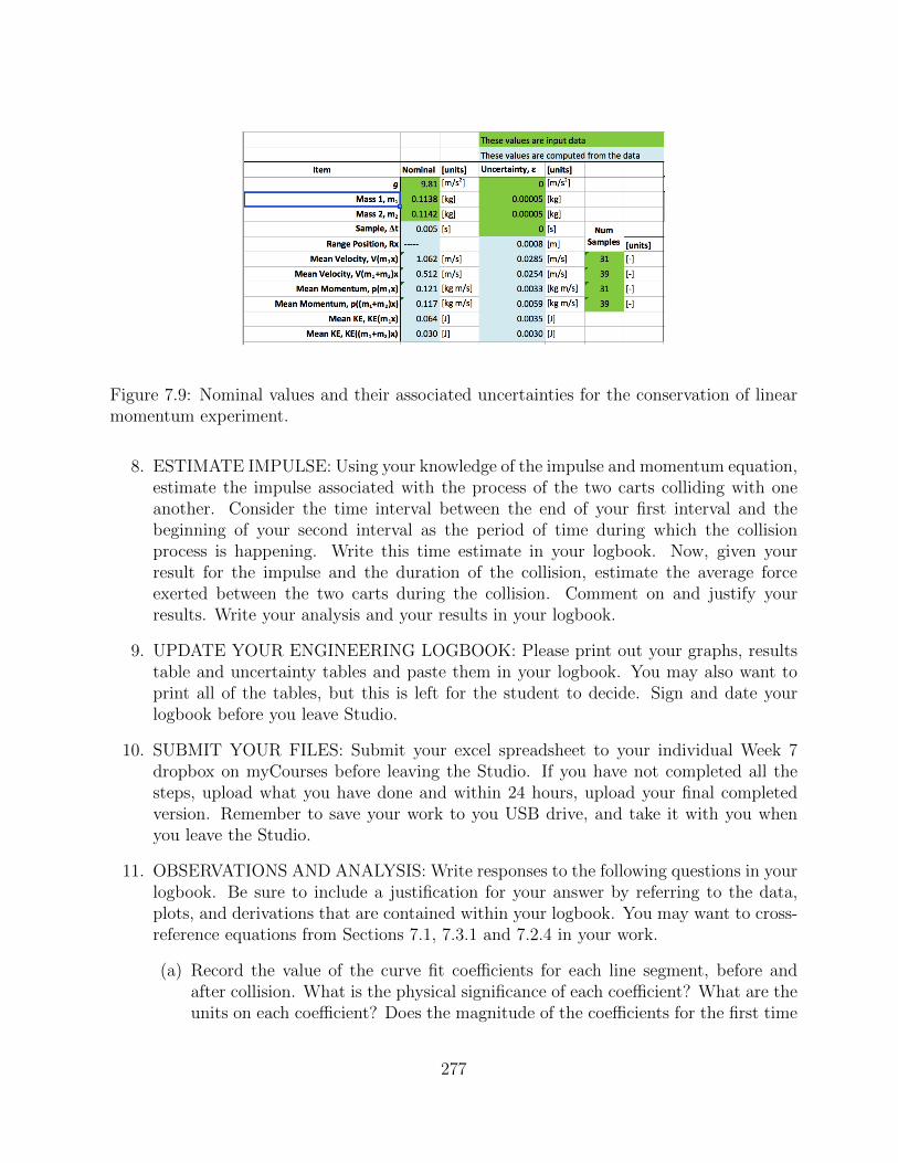
Figure 7.9: Nominal values and their associated uncertainties for the conservation of linearmomentum experiment.
8. ESTIMATE IMPULSE: Using your knowledge of the impulse and momentum equation,estimate the impulse associated with the process of the two carts colliding with oneanother. Consider the time interval between the end of your first interval and thebeginning of your second interval as the period of time during which the collisionprocess is happening. Write this time estimate in your logbook. Now, given yourresult for the impulse and the duration of the collision, estimate the average forceexerted between the two carts during the collision. Comment on and justify yourresults. Write your analysis and your results in your logbook.
9. UPDATE YOUR ENGINEERING LOGBOOK: Please print out your graphs, resultstable and uncertainty tables and paste them in your logbook. You may also want toprint all of the tables, but this is left for the student to decide. Sign and date yourlogbook before you leave Studio.
10. SUBMIT YOUR FILES: Submit your excel spreadsheet to your individual Week 7dropbox on myCourses before leaving the Studio. If you have not completed all thesteps, upload what you have done and within 24 hours, upload your final completedversion. Remember to save your work to you USB drive, and take it with you whenyou leave the Studio.
11. OBSERVATIONS AND ANALYSIS: Write responses to the following questions in yourlogbook. Be sure to include a justification for your answer by referring to the data,plots, and derivations that are contained within your logbook. You may want to cross-reference equations from Sections 7.1, 7.3.1 and 7.2.4 in your work.
(a) Record the value of the curve fit coe�cients for each line segment, before andafter collision. What is the physical significance of each coe�cient? What are theunits on each coe�cient? Does the magnitude of the coe�cients for the first time
277
interval appear to be physically consistent with Newton’s Law when compared tothe magnitude and sign of the coe�cients for the second time interval? Why orwhy not?
(b) Describe and quantify the sources of error in your calculations. Which uncertain-ties contributed the most to the accuracy of the results? What would you do ifasked to minimize this error in future experiments?
(c) How do your findings show agreement or disagreement with the Work EnergyThereom?
(d) How do your findings show agreement or disagreement with the Conservation ofLinear Momentum?
12. CONGRATULATIONS! You have just completed the Studio portion for week 7.
13. WRITE THE REPORT: Please refer to section 7.3.3 Report on details for the reportsubmission. Before leaving Studio, decide on a date and time to meet up with yourteam mates to prepare the report. Reports are due Monday by 6 pm.
7.3.3 Report
Please use the same task distribution for writing the report that was outlined in Week 1, withthe additional responsibility of the conclusion section for the scribe. Remember, however,that all team members should contribute to and approve the quality of the report as well asensure a timely submission.
Prepare a report to include only the following components:
1. TITLE PAGE: This is the title page. Include the title of your experiment “Conser-vation of Linear Momentum”, Team Number, date, team member names, and teammember roles for the week. The team scribe should be listed as the first author. Includeone small photograph of each team member showing them posed with their apparatusfor the students’ trials. Include the student name and their m
1
, m2
configuration as acaption on each photo.
2. PAGE 1: The heading on this page should read Experimental Set-up. Create adiagram of the experimental set-up. This week we will include only the diagram andits caption. Thus, is it important that your diagram clearly communicate the set-up,including each key component and where measurements were taken. The importantinformation to communicate are the variable names and datums that relate to yourmeasurements and results. It is a good practice to add a legend that defines anyvariables or components of the schematic that are not obvious. At the bottom of thefigure include a figure caption, for example Figure 1. A brief figure caption. Referto the text for examples.
278
Note: Figure captions are required for every plot and diagram in the report, exceptfor the title page. Figure captions are placed below the figures, and are numberedsequentially beginning with Figure 1 for the first figure in the report.
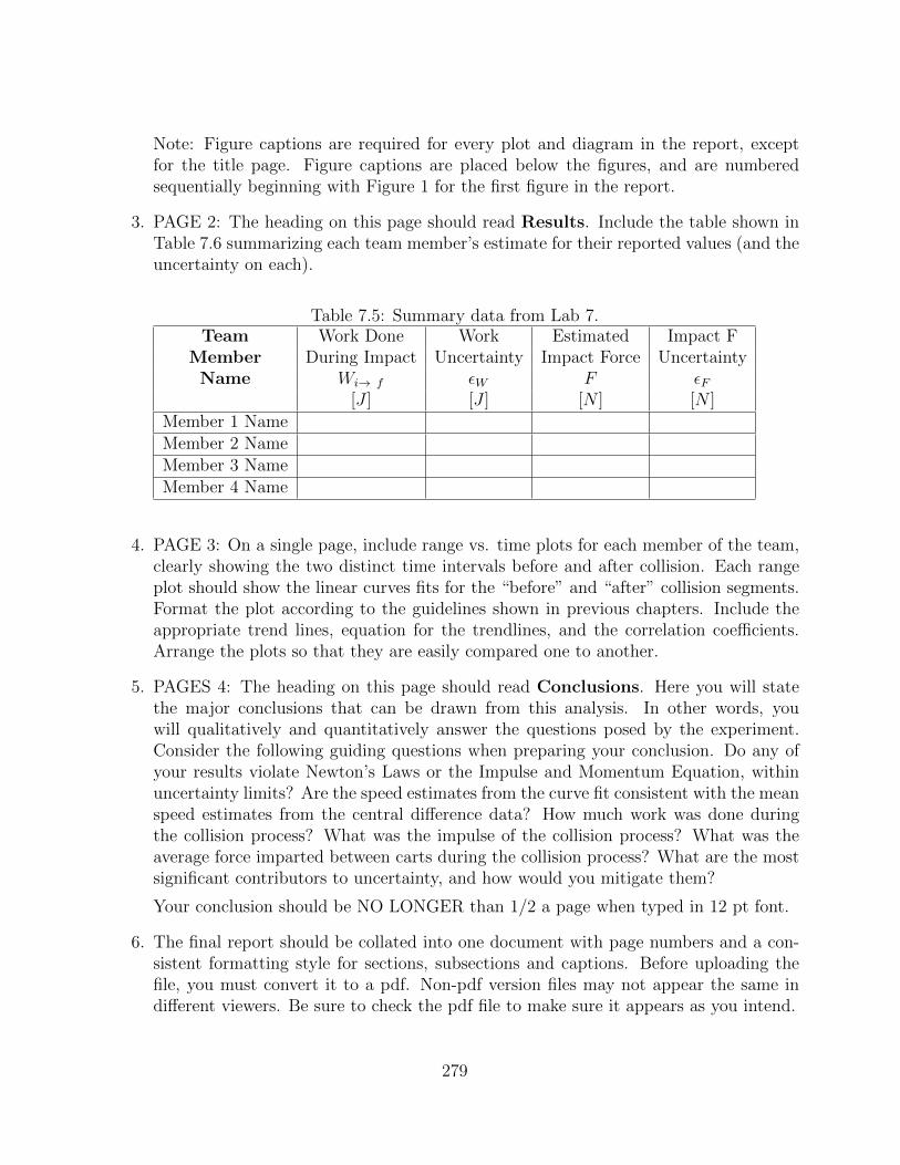
3. PAGE 2: The heading on this page should read Results. Include the table shown inTable 7.6 summarizing each team member’s estimate for their reported values (and theuncertainty on each).
Table 7.5: Summary data from Lab 7.Team Work Done Work Estimated Impact F
Member During Impact Uncertainty Impact Force UncertaintyName Wi! f ✏W F ✏F
[J ] [J ] [N ] [N ]Member 1 NameMember 2 NameMember 3 NameMember 4 Name
4. PAGE 3: On a single page, include range vs. time plots for each member of the team,clearly showing the two distinct time intervals before and after collision. Each rangeplot should show the linear curves fits for the “before” and “after” collision segments.Format the plot according to the guidelines shown in previous chapters. Include theappropriate trend lines, equation for the trendlines, and the correlation coe�cients.Arrange the plots so that they are easily compared one to another.
5. PAGES 4: The heading on this page should read Conclusions. Here you will statethe major conclusions that can be drawn from this analysis. In other words, youwill qualitatively and quantitatively answer the questions posed by the experiment.Consider the following guiding questions when preparing your conclusion. Do any ofyour results violate Newton’s Laws or the Impulse and Momentum Equation, withinuncertainty limits? Are the speed estimates from the curve fit consistent with the meanspeed estimates from the central di↵erence data? How much work was done duringthe collision process? What was the impulse of the collision process? What was theaverage force imparted between carts during the collision process? What are the mostsignificant contributors to uncertainty, and how would you mitigate them?
Your conclusion should be NO LONGER than 1/2 a page when typed in 12 pt font.
6. The final report should be collated into one document with page numbers and a con-sistent formatting style for sections, subsections and captions. Before uploading thefile, you must convert it to a pdf. Non-pdf version files may not appear the same indi↵erent viewers. Be sure to check the pdf file to make sure it appears as you intend.
279

7.4 Recitation
Recitation this week will focus on problem solving. Please come prepared, with your attemptsat the homework problem already in your logbooks.
280

7.5 Homework Problems
Complete all assigned homework problems in your logbook.
7.5.1 Given a first cart having momentum �!p1
= (1ı̂+1|̂+1k̂)[Ns] and a second cart havingmomentum �!p
2
= (1ı̂ + 1|̂ + 1k̂)[Ns], which collide and attach in a frictionless, elasticcollision, find the momentum of the combined carts following the collision.
7.5.2 Given a first cart having momentum �!p1
= (1ı̂+1|̂+1k̂)[Ns] and a second cart havingmomentum �!p
2
= (�1ı̂� 1|̂� 1k̂)[Ns], which collide and attach in a frictionless, elasticcollision, find the momentum of the combined carts following the collision.
7.5.3 Given a first cart having momentum �!p1
= 1ı̂ + 1|̂ + 1k̂[Ns] and a second cart havingmomentum �!p
2
= �1ı̂+(�1)|̂�1k̂[Ns], which collide and attach in a frictionless, elasticcollision, find the momentum of the combined carts following the collision.
7.5.4 Given a first cart having momentum �!p1
= 4ı̂ + 3|̂ � 6k̂[Ns] and a second cart havingmomentum �!p
2
= 1ı̂ � 4|̂ + 8k̂[Ns], which collide and attach in a frictionless, elasticcollision, find the momentum of the combined carts following the collision.
7.5.5 Given a first cart having momentum �!p1
= 4ı̂ + 3|̂ � 6k̂[Ns] and a second cart havingmomentum �!p
2
= 0ı̂ � 1|̂ + 0k̂[Ns], which collide and attach in a frictionless, elasticcollision, find the momentum of the combined carts following the collision.
7.5.6 Given a first cart having momentum �!p1
= 4ı̂ + 3|̂ � 6k̂[Ns] and a second cart havingmomentum �!p
2
= 1ı̂ + 0|̂ + 0k̂[Ns], which collide and attach in a frictionless, elasticcollision, find the momentum of the combined carts following the collision.
7.5.7 Given a first cart having momentum �!p1
= 4ı̂ + 3|̂ � 6k̂[Ns] and a second cart havingmomentum �!p
2
= 0ı̂ + 1|̂ + 0k̂[Ns], which collide and attach in a frictionless, elasticcollision, find the momentum of the combined carts following the collision.
7.5.8 Given a first cart having momentum �!p1
= 4ı̂ + 3|̂ � 6k̂[Ns] and a second cart havingmomentum �!p
2
= 0ı̂ + 0|̂ + 1k̂[Ns], which collide and attach in a frictionless, elasticcollision, find the momentum of the combined carts following the collision.
7.5.9 Given a first cart having momentum �!p1
= 4ı̂ + 3|̂ � 6k̂[Ns] and a second cart havingmomentum �!p
2
= �1ı̂ + 0|̂ + 0k̂[Ns], which collide and attach in a frictionless, elasticcollision, find the momentum of the combined carts following the collision.
7.5.10 Given a first cart having momentum �!p1
= 4ı̂ + 3|̂ � 6k̂[Ns] and a second cart havingmomentum �!p
2
= 0ı̂ � 1|̂ + 0k̂[Ns], which collide and attach in a frictionless, elasticcollision, find the momentum of the combined carts following the collision.
281
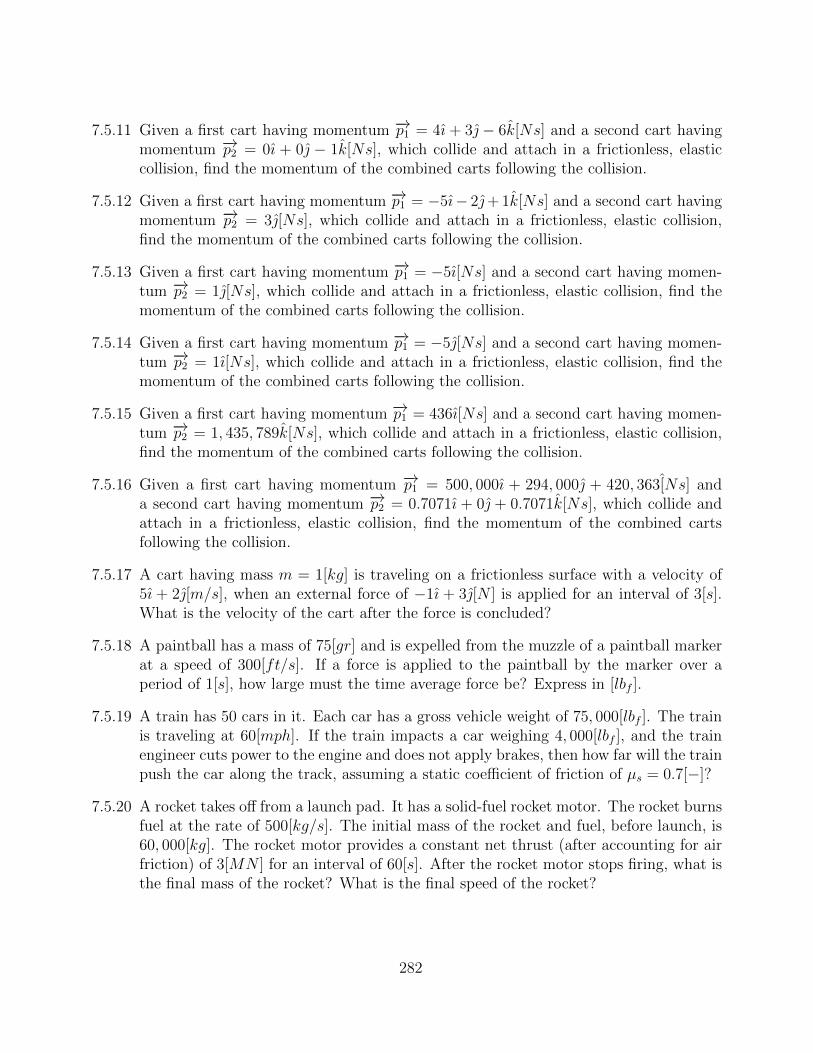
7.5.11 Given a first cart having momentum �!p1
= 4ı̂ + 3|̂ � 6k̂[Ns] and a second cart havingmomentum �!p
2
= 0ı̂ + 0|̂ � 1k̂[Ns], which collide and attach in a frictionless, elasticcollision, find the momentum of the combined carts following the collision.
7.5.12 Given a first cart having momentum �!p1
= �5ı̂� 2|̂+1k̂[Ns] and a second cart havingmomentum �!p
2
= 3|̂[Ns], which collide and attach in a frictionless, elastic collision,find the momentum of the combined carts following the collision.
7.5.13 Given a first cart having momentum �!p1
= �5ı̂[Ns] and a second cart having momen-tum �!p
2
= 1|̂[Ns], which collide and attach in a frictionless, elastic collision, find themomentum of the combined carts following the collision.
7.5.14 Given a first cart having momentum �!p1
= �5|̂[Ns] and a second cart having momen-tum �!p
2
= 1ı̂[Ns], which collide and attach in a frictionless, elastic collision, find themomentum of the combined carts following the collision.
7.5.15 Given a first cart having momentum �!p1
= 436ı̂[Ns] and a second cart having momen-tum �!p
2
= 1, 435, 789k̂[Ns], which collide and attach in a frictionless, elastic collision,find the momentum of the combined carts following the collision.
7.5.16 Given a first cart having momentum �!p1
= 500, 000ı̂ + 294, 000|̂ + 420, 363̂[Ns] anda second cart having momentum �!p
2
= 0.7071ı̂ + 0|̂ + 0.7071k̂[Ns], which collide andattach in a frictionless, elastic collision, find the momentum of the combined cartsfollowing the collision.
7.5.17 A cart having mass m = 1[kg] is traveling on a frictionless surface with a velocity of5ı̂ + 2|̂[m/s], when an external force of �1ı̂ + 3|̂[N ] is applied for an interval of 3[s].What is the velocity of the cart after the force is concluded?
7.5.18 A paintball has a mass of 75[gr] and is expelled from the muzzle of a paintball markerat a speed of 300[ft/s]. If a force is applied to the paintball by the marker over aperiod of 1[s], how large must the time average force be? Express in [lbf ].
7.5.19 A train has 50 cars in it. Each car has a gross vehicle weight of 75, 000[lbf ]. The trainis traveling at 60[mph]. If the train impacts a car weighing 4, 000[lbf ], and the trainengineer cuts power to the engine and does not apply brakes, then how far will the trainpush the car along the track, assuming a static coe�cient of friction of µs = 0.7[�]?
7.5.20 A rocket takes o↵ from a launch pad. It has a solid-fuel rocket motor. The rocket burnsfuel at the rate of 500[kg/s]. The initial mass of the rocket and fuel, before launch, is60, 000[kg]. The rocket motor provides a constant net thrust (after accounting for airfriction) of 3[MN ] for an interval of 60[s]. After the rocket motor stops firing, what isthe final mass of the rocket? What is the final speed of the rocket?
282