Chapter 7 Remote Sensing-Based Monitoring of Potential Climate-Induced Impacts on Habitats · 2017-08-27 · Remote Sensing-Based Monitoring of Potential Climate-Induced Impacts on

Chapter 7

Remote Sensing-Based Monitoringof Potential Climate-Induced Impactson Habitats

Michael Forster, Marc Zebisch, Iris Wagner-Lucker, Tobias Schmidt,Kathrin Renner, and Marco Neubert

7.1 Introduction

Climate change is likely to be a strong driver of changes in habitat conditions and,

subsequently, species composition. Sensitive and accurate monitoring techniques

are required to reveal changes in protected areas and habitats. Remote sensing bears

the potential to fulfil these requirements because it provides a broad view of

landscapes and offers the opportunity to acquire data in a systematic, repeatable,

and spatially explicit manner. It is an important tool for monitoring and managing

habitats and protected areas as it allows the acquisition of data in remote and

inaccessible areas. This is important since traditional field-based biodiversity assess-

ment methods (although far more detailed and often more accurate) are sometimes

subjective and usually spatially restrained due to constraints in time, finance, or

habitat accessibility. Remote sensing can provide indicators for different spatial and

M. Forster (*) • T. Schmidt

Geoinformation in Environmental Planning Lab, Department of Landscape

Architecture and Environmental Planning, Technical University of Berlin,

Str. d. 17. Juni 145, 10623 Berlin, Germany

e-mail: [email protected]

M. Zebisch • K. Renner

Institute for Applied Remote Sensing, EURAC Research, Viale Druso 1, 39100 Bolzano, Italy

I. Wagner-Lucker

Department of Conservation Biology, Vegetation- and Landscape Ecology,

University of Vienna, Rennweg 14, 1030 Vienna, Austria

Department of Limnology, University of Vienna, Althanstrasse 14, 1090 Vienna, Austria


M. Neubert

Leibniz Institute of Ecological Urban and Regional Development,

Weberplatz 1, 01217 Dresden, Germany


S. Rannow and M. Neubert (eds.), Managing Protected Areas in Centraland Eastern Europe Under Climate Change, Advances in Global Change Research 58,

DOI 10.1007/978-94-007-7960-0_7, © The Author(s) 2014

95

mailto:[email protected]



temporal scales ranging from the individual habitat level to entire landscapes and

involving varying temporal revisit frequencies up to daily observations.

Habitat mapping is developing at a fast ratewithin the two basic approaches of field

mapping and remote sensing. The latest technologies are quickly incorporated into

habitat monitoring (Lengyel et al. 2008; Turner et al. 2003). Field mapping, for

example, is facilitated by the use of object-oriented methods or wireless sensor

systems (e.g. Polastre et al. 2004; Bock et al. 2005). Additionally, advances in remote

sensing methods have resulted in the widespread production and use of spatial

information on biodiversity (Duro et al. 2007; Papastergiadou et al. 2007; Forster

et al. 2008). In fact, earth observation data is becoming more and more accepted as an

appropriate data source to supplement, and in some cases even replace, field-based

surveys in biodiversity science and conservation, as well as in ecology. Objectivity

and transparency in the process of integrity assessments of Natura 2000 sites can be

supported by quantitative methods, if applied cautiously (Lang and Langanke 2005).

However, it should be kept in mind that there are various sources of uncertainty in

remote sensing-based monitoring of vegetation (Rocchini et al. 2013).

Despite all the advantages mentioned above, the monitoring of habitats using field-

based and remote sensing approaches has a very short history. Landsat-4, the first

non-military optical sensor with the potential to monitor habitats at a suitable spatial

resolution, was initiated only in 1982. Even within this time period the story of image

acquisition and interpretation is not free of interruptions due to sensor faults and a lack

of financial support for continuity missions (Wulder et al. 2011). Recently, the sensor

series RapidEye and the planned mission Sentinel-2, which employ a constellation of

multiple identical satellites, have been supplying data with a higher temporal fre-

quency (Berger et al. 2012). However, this time-span is still not long enough to allow

reliable statements about modifications of habitats dependent on climate change.

This study focuses on the potential of remote sensing to detect indicators related

to climate change in three focus areas. The case studies presented use the Natura

2000 habitat nomenclature and descriptions of the conservation status of the

protected habitats as a basis for their evaluation. For all studies within this chapter,

RapidEye products acquired between 2009 and 2011 were used as basic imagery for

the subsequent investigations due to their frequent availability and suitable spectral

as well as spatial resolution. The acquired images were always used in combination

for a single mapping step. The necessary time-frame for monitoring with repeated

image acquisition (e.g. a 6-year cycle as proposed in the EC Habitats Directive) was

not available within the HABIT-CHANGE project.

Within the general framework described (Natura 2000-related indicators,

RapidEye data from 2009 to 2011), methods for various habitats in three different

biogeographic regions (Continental, Alpine, Pannonian) were applied. The tech-

niques, which are described in the following subchapters, are intended to demonstrate

their potential for indicating likely climate change impacts. In the Vessertal, a

forested area in Germany, the immigration of beech into a spruce dominated region –

a potential effect of climate change – was investigated (Sect. 7.2). In the Lake

Neusiedl area in Austria potential climate-induced changes in Pannonic inland

marshes are shown (Sect. 7.3). In Rieserferner Ahrn, an Alpine region in Italy, the

potential of detecting shrub encroachment – an indicator for climate-related change to

the treeline – was explored (Sect. 7.4).

96 M. Forster et al.

7.2 Case Study Forest Habitats: Vessertal, Germany

A detailed description of the study area Vessertal is found in Sect. 16.2. In Chap. 16,

climate change related sensitivity of forests in general and the Vessertal specifically

is also described. This section, therefore, provides only a summary of the main facts

of the region. With 88 % forest cover, the Biosphere Reserve Vessertal can be

characterised as a landscape almost completely covered by woodland. The main

tree types are spruce and beech. In terms of protected habitats Luzulo-Fagetumbeech forests (habitat code 9110) and Asperulo-Fagetum beech forests (habitat

code 9130) are of major importance (see Table 16.1).

As already mentioned above, only a long-term study can provide facts about the

immigration of beeches into spruce dominated areas as may be occurring in the

Vessertal region. However, the multi-temporal based short-term habitat quality

indicator presented here can be used to detect the actual status of tree species

compositions within the protected areas. Using this approach a detailed and accu-

rate differentiation of tree species can be obtained. Knowledge about the current

status of the tree population is important information for decision makers, helping

them plan further management measures for conservation of the Natura 2000

habitat types.

7.2.1 Data and Methods

For this study a multi-temporal series of RapidEye data (Level 3A) for the study area

Biosphere Reserve Vessertal (Table 7.1) was obtained in 2011. Four images with the

acquisition dates 24-04-2011, 08-05-2011, 26-08-2011, and 23-10-2011 were avail-

able. The RapidEye mission represents a constellation of five satellites and provides

high spatial resolution multi-temporal imagery. Five optical bands cover a range of

400–850 nm, whereby the first three bands represent the visible spectral range

(400–685 nm). Band 4 covers the red-edge wavelength (690–730 nm), which is

very sensitive for vegetation chlorophyll, and band 5 covers the near-infrared

(760–850 nm). The spatial resolution is 6.5 m for level 1B data and resampled to

5 m for orthorectified level 3A data (Schuster et al. 2012).

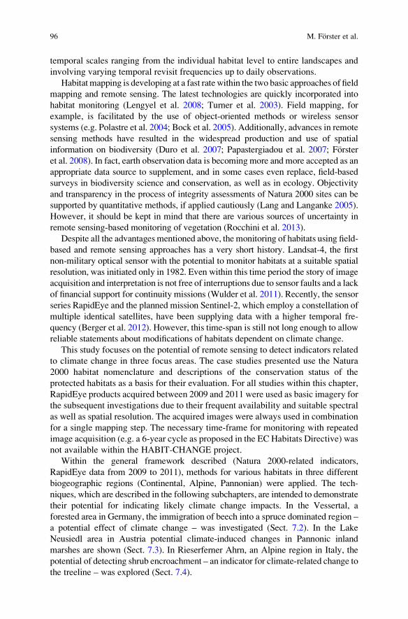
Table 7.1 Percentage of the share of natural tree types as an example indicator for the determi-

nation of conservation status for Luzulo Fagetum beech forests and Asperulo Fagetum beech

forests (�90 % beech ¼ favourable; between 80 and 90 % beech ¼ unfavourable – inadequate;

below 80 % beech ¼ unfavourable – bad). The areas reported as Asperulo Fagetum beech forests

show a higher share of favourable conservation status than Luzulo Fagetum beech forests

Conservation status Luzulo Fagetum (9110) Asperulo Fagetum (9130)

Favourable 14.19 % 57.68 %

Unfavourable – inadequate 30.61 % 37.73 %

Unfavourable – bad 55.19 % 4.58 %

7 Remote Sensing-Based Monitoring of Potential Climate-Induced Impacts on Habitats 97

http://dx.doi.org/10.1007/978-94-007-7960-0_16

http://dx.doi.org/10.1007/978-94-007-7960-0_16

http://dx.doi.org/10.1007/978-94-007-7960-0_16

The pre-processing of the images included geometric correction (image-to-image)

and radiometric normalisation to a cloud-free reference image in the middle of the

vegetation period with a high radiometric quality (RapidEye image from 26-08-2011)

to adjust the spectral variability. The IR-MAD algorithm implemented in ENVI/IDL

was used for the radiometric normalisation. This algorithm automatically detects

no-change pixels based on a no-change probability threshold and performs a relative

radiometric normalisation of the images (Canty and Nielsen 2008).

Since the spatial accuracy of additionally available forest inventory data was

insufficient to generate training samples for a supervised tree species classification,

an unsupervised Isodata classification was performed in order to allocate spectral

homogeneous clusters. These clusters were visually interpreted using aerial photo-

graphs and attributed to the classes beech, spruce, or open landscape. Subsequently,

for each class, 1,000 random sample points were generated based on these spectral

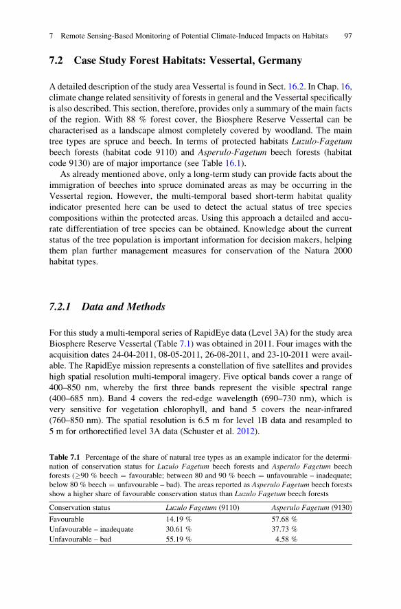
homogeneous areas. From these extracted sample points, a supervised classification,

based on multi-temporal data using the Support Vector Machine (SVM) algorithm

(Karatzoglou et al. 2005), was performed to generate a thematic tree species map

(Fig. 7.1). For this process the samples were portioned into 70 % for the training of

the SVM and 30% for the validation. Thereafter, the tree species map was intersected

with each of the existing Natura 2000 habitat type boundaries, which were available

as a field-based mapping GIS-layer for reporting purposes from the Vessertal Bio-

sphere Reserve. The tree species compositions (beech/spruce) per polygon

were computed based on this independent data source.

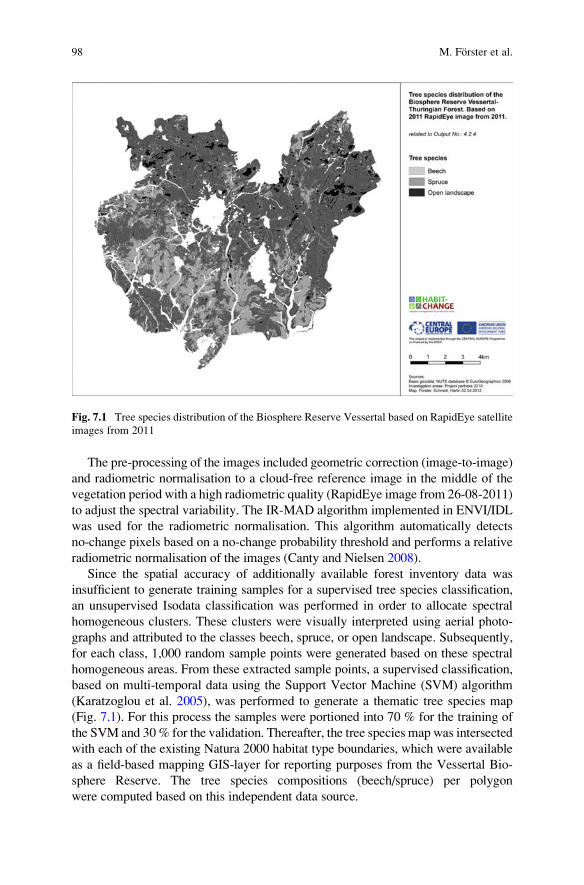
Fig. 7.1 Tree species distribution of the Biosphere Reserve Vessertal based on RapidEye satellite

images from 2011


This approach enables detailed monitoring of habitat quality related to the tree

species compositions. In terms of Natura 2000 in Germany, objective mapping

guidelines with defined rules are available to determine the conservation status of a

forest habitat (Burkhardt et al. 2004). These parameters define the status of a specific

Natura 2000 site (e.g. favourable, unfavourable – inadequate, or unfavourable – bad).

One indicator, suitable for remote sensing applications, is the percentage of natural

forest types in terms of the abundance of specific species (Forster and Kleinschmit

2008). For this indicator, the tree species composition per polygon was calculated.

7.2.2 Results

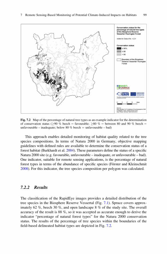
The classification of the RapidEye images provides a detailed distribution of the

tree species in the Biosphere Reserve Vessertal (Fig. 7.1). Spruce covers approx-

imately 62 %, beech 30 %, and open landscape 8 % of the study site. The overall

accuracy of the result is 88 %, so it was accepted as accurate enough to derive the

indicator “percentage of natural forest types” for the Natura 2000 conservation

status. The results of the percentage of tree species within the boundaries of the

field-based delineated habitat types are depicted in Fig. 7.2.

Fig. 7.2 Map of the percentage of natural tree types as an example indicator for the determination

of conservation status (�90 % beech ¼ favourable; �80 % ¼ between 80 and 90 % beech ¼unfavourable – inadequate; below 80 % beech ¼ unfavourable – bad)


In an exemplary evaluation of the conservation status for Luzulo Fagetum beech

forests and Asperulo Fagetum beech forests, relying just on this single indicator, it

can be shown that the conservation status of Asperulo Fagetum is more often

favourable than for Luzulo Fagetum (Table 7.1), which corresponds with the

findings of the field-based mapping presented in Chap. 16.

7.2.3 Conclusions

The results of the case study Vessertal illustrate the successful evaluation of an

indicator of the conservation status of continental forest habitats (percentage of

natural tree types). However, not all indicators defined for the conservation status of

woodlands in Germany are detectable with RapidEye imagery. The differentiation

of habitat types often relies on the understorey vegetation, which is not detectable

using earth observation techniques. Within forest habitats a combination with

LiDAR (Light Detection and Ranging) techniques has proven to be relatively

helpful (Vehmas et al. 2009). However, the exploration of a set of indicators

detectable by remote sensing that may complement the field-based data-set remains

under discussion. In terms of climate change, the indicator evaluated here, percent-

age of natural tree types, can be utilised to monitor the immigration of beech into a

spruce dominated region of the Thuringian Forest.

7.3 Case Study Wetland Habitats: Lake Neusiedl, Austria

7.3.1 Study Area

The transboundary Lake Neusiedl/Ferto-Hangsag National Park was founded in

1993. It is situated at the Austrian and Hungarian border (see Fig. 1.1). Lake

Neusiedl itself is – in hydrological terms – a steppe lake, the westernmost of a

series of steppe lakes extending throughout Eurasia. It is especially sensitive to

climate variations due to its extreme shallowness and small catchment area. His-

torical records indicate that large variations of the lake area have occurred natu-

rally. However, today a constant water level is maintained by water engineering

measures. Considering future climate scenarios, the main risk for Lake Neusiedl is

significant water losses that could enhance eutrophication and algal growth (Soja

et al. 2013).

East of the lake approximately 80 shallow saline ponds can be found. Nowadays,

this area is determined by the spread of reed stands, smaller ponds created by the

interconnection of the former bay-type formations, and smaller bays. Furthermore,

reed in general is the most characteristic habitat in the region, covering more than

70 % of the protected area. Its structure ranges from very dense and impassable to


http://dx.doi.org/10.1007/978-94-007-7960-0_16

http://dx.doi.org/10.1007/978-94-007-7960-0_1

sparse stands mixed with stretches of open water. In addition to reed, inland

marshes (habitat code: 1530* – the star indicates a priority habitat) and calcareous

fens (habitat codes: 7210 & 7230*) can be found in this region. In contrast to the

larger patches of reed, these habitats are considered to be of European importance

in terms of the EC Habitats Directive.


For this case study two RapidEye images from 2009 (April and August, Level 3A),

a Digital Elevation Model (DEM) to detect small altitude differences, and CORINE

Land Cover data were used.

Within the European Union inland marshes are found solely in the region of

Lake Neusiedl. They are greatly disturbed by increased nutrition input, changes in

hydrology, regrowth of atypical plant types, and a decrease of land-use or degra-

dation through intensive land-use. Some of these disturbances can be related to

climate-induced impacts (e.g. change in moisture conditions). The Environmental

Agency Austria uses an indicator-based approach to evaluate the quality of these

habitats. The indicators employed are area, species composition, hydrology, com-

pleteness of typical habitat structures, and presence of disturbance indicator plant

species. Here, a similar approach is used to develop potential habitat maps to

support the monitoring process and consequently to detect areas not known to be

covered by inland marshes. Because most of these indicators cannot be derived

from satellite data, moisture and biomass were used for this investigation.

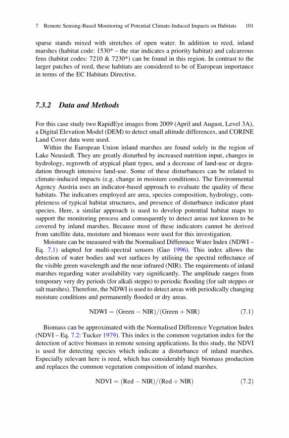
Moisture can be measured with the Normalised Difference Water Index (NDWI –

Eq. 7.1) adapted for multi-spectral sensors (Gao 1996). This index allows the

detection of water bodies and wet surfaces by utilising the spectral reflectance of

the visible green wavelength and the near infrared (NIR). The requirements of inland

marshes regarding water availability vary significantly. The amplitude ranges from

temporary very dry periods (for alkali steppe) to periodic flooding (for salt steppes or

salt marshes). Therefore, the NDWI is used to detect areas with periodically changing

moisture conditions and permanently flooded or dry areas.

NDWI ¼ Green� NIRð Þ= Greenþ NIRð Þ ð7:1Þ

Biomass can be approximated with the Normalised Difference Vegetation Index

(NDVI – Eq. 7.2: Tucker 1979). This index is the common vegetation index for the

detection of active biomass in remote sensing applications. In this study, the NDVI

is used for detecting species which indicate a disturbance of inland marshes.

Especially relevant here is reed, which has considerably high biomass production

and replaces the common vegetation composition of inland marshes.

NDVI ¼ Red� NIRð Þ= Redþ NIRð Þ ð7:2Þ


Additionally, a DEM with a spatial resolution of 5 m and a ground depression

detection map were used. Since especially salt steppes and salt marshes are closely

related to the ground or sea water level, it can be assumed that ground depressions

provide a high potential for this habitat type. The same applies to littoral zones

beside the lake. However, littoral zones are not detected as ground depressions,

since the entire littoral zone is already depressed. To determine these waterside

areas, all areas between the lake’s average surface of 115.45 m and 116 m ground

elevation are taken as littoral zones.

Thresholds were applied to estimate three probability levels of inland marshes

(Fig. 7.3). These thresholds are derived from reference habitats to deduce high,

medium, and low habitat occurrence probabilities. Only land-cover types with a

realistic potential for inland marshes were considered for the application of the rule

set. CORINE land-cover data were used to mask out land-cover classes with little

potential (e.g. urban areas).

7.3.3 Results

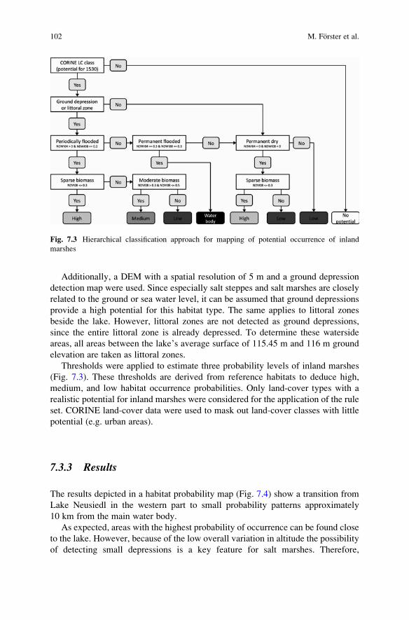
The results depicted in a habitat probability map (Fig. 7.4) show a transition from

Lake Neusiedl in the western part to small probability patterns approximately

10 km from the main water body.

As expected, areas with the highest probability of occurrence can be found close

to the lake. However, because of the low overall variation in altitude the possibility

of detecting small depressions is a key feature for salt marshes. Therefore,

Fig. 7.3 Hierarchical classification approach for mapping of potential occurrence of inland

marshes


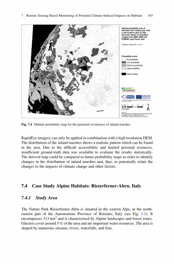
RapidEye imagery can only be applied in combination with a high resolution DEM.

The distribution of the inland marshes shows a realistic pattern which can be found

in the area. Due to the difficult accessibility and limited personal resources,

insufficient ground-truth data was available to evaluate the results statistically.

The derived map could be compared to future probability maps in order to identify

changes in the distribution of inland marshes and, thus, to potentially relate the

changes to the impacts of climate change and other factors.

7.4 Case Study Alpine Habitats: Rieserferner-Ahrn, Italy

7.4.1 Study Area

The Nature Park Rieserferner-Ahrn is situated in the eastern Alps, in the north-

eastern part of the Autonomous Province of Bolzano, Italy (see Fig. 1.1). It

encompasses 313 km2 and is characterised by Alpine landscapes and forest zones.

Glaciers cover around 5 % of the area and are important water resources. The area is

shaped by numerous streams, rivers, waterfalls, and fens.

Fig. 7.4 Habitat probability map for the potential occurrence of inland marshes


http://dx.doi.org/10.1007/978-94-007-7960-0_1

The location in the inner Alps south of the Alpine divide renders the climate

moderately dry. The study area covers an elevation range from 890 to 3,480 m

above mean sea-level. The vegetation reflects the mountainous character of the

nature park. Spruce forests dominate while the timber line is made up of larch and

Swiss pine. Increasing in altitude, the vegetation is composed of Alpine meadows

and sub-Alpine and Alpine small shrubs and heath. Extreme habitats for plants and

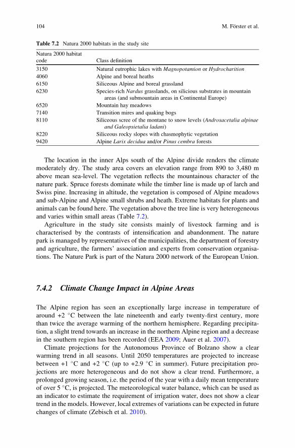
animals can be found here. The vegetation above the tree line is very heterogeneous

and varies within small areas (Table 7.2).

Agriculture in the study site consists mainly of livestock farming and is

characterised by the contrasts of intensification and abandonment. The nature

park is managed by representatives of the municipalities, the department of forestry

and agriculture, the farmers’ association and experts from conservation organisa-

tions. The Nature Park is part of the Natura 2000 network of the European Union.

7.4.2 Climate Change Impact in Alpine Areas

The Alpine region has seen an exceptionally large increase in temperature of

around +2 �C between the late nineteenth and early twenty-first century, more

than twice the average warming of the northern hemisphere. Regarding precipita-

tion, a slight trend towards an increase in the northern Alpine region and a decrease

in the southern region has been recorded (EEA 2009; Auer et al. 2007).

Climate projections for the Autonomous Province of Bolzano show a clear

warming trend in all seasons. Until 2050 temperatures are projected to increase

between +1 �C and +2 �C (up to +2.9 �C in summer). Future precipitation pro-

jections are more heterogeneous and do not show a clear trend. Furthermore, a

prolonged growing season, i.e. the period of the year with a daily mean temperature

of over 5 �C, is projected. The meteorological water balance, which can be used as

an indicator to estimate the requirement of irrigation water, does not show a clear

trend in the models. However, local extremes of variations can be expected in future

changes of climate (Zebisch et al. 2010).

Table 7.2 Natura 2000 habitats in the study site

Natura 2000 habitat

code Class definition

3150 Natural eutrophic lakes with Magnopotamion or Hydrocharition

4060 Alpine and boreal heaths

6150 Siliceous Alpine and boreal grassland

6230 Species-rich Nardus grasslands, on silicious substrates in mountain

areas (and submountain areas in Continental Europe)

6520 Mountain hay meadows

7140 Transition mires and quaking bogs

8110 Siliceous scree of the montane to snow levels (Androsacetalia alpinaeand Galeopsietalia ladani)

8220 Siliceous rocky slopes with chasmophytic vegetation

9420 Alpine Larix decidua and/or Pinus cembra forests


The largest pressure on habitats in Alpine areas is land-use. This is true despite

land-use activities being limited within the Nature Park due to conservation

restrictions. Pressures arise mostly from extensive forestry, agriculture (grass-

lands with livestock breeding and pasture farming), tourism, and traffic. In this

study we investigated the following potential impacts for the study area

Rieserferner Ahrn:

• increase in dwarf shrub cover,

• change in tree line,

• new vegetation on rocks and the glacier forefields,

• changes in water regime and intra-annual and inter-annual dynamics,

• changes in phenology and its intra-annual and inter-annual dynamics (Zebisch

et al. 2010).


For the study area four RapidEye images (Level 1B) with the acquisition dates

22-07-2009, 29-07-2009, 03-10-2009 and 31-07-2010 were available. The follow-

ing auxiliary data sets were used:

• a colour aerial orthophoto acquired in 2006 with a spatial resolution of 0.5 m,

• a Digital Elevation Model (DEM) with a spatial resolution of 2.5 m,

• solar radiation layers – from RapidEye images using metadata and DEM,

• texture layers: texture features (Haralick et al. 1973) such as mean, variance,

homogeneity, contrast, dissimilarity, entropy, second angular moment and cor-

relation features were generated from the orthophoto,

• detailed habitat thematic map: field mapping 2006 as well as photointerpretation

and digitalisation of orthophotos by experts.

Initially the RapidEye images were orthorectified (Toutin 2003) and the pixel

values converted to reflectance at top of the atmosphere (TOA). In the latter step

only distance to the sun and the geometry of the incoming solar radiation was

considered. Next we masked out clouds and shadowed areas in the images using

object-based image analysis. Using Definiens eCognition software the images were

first segmented and classified into two levels to map clouds and shadows based on

object statistics, topological and shape object’s features. The mapping results of the

two classification levels were then merged. The classification was further improved

by modifications of the object’s shapes using appropriate features of classified

objects. Subsequently, training as well as validation samples of the different

vegetation types were derived following a random stratified sampling approach

based on thematically homogeneous areas. A minimum of 50 samples were taken

from twelve vegetation types present in the study area. The SVM classification


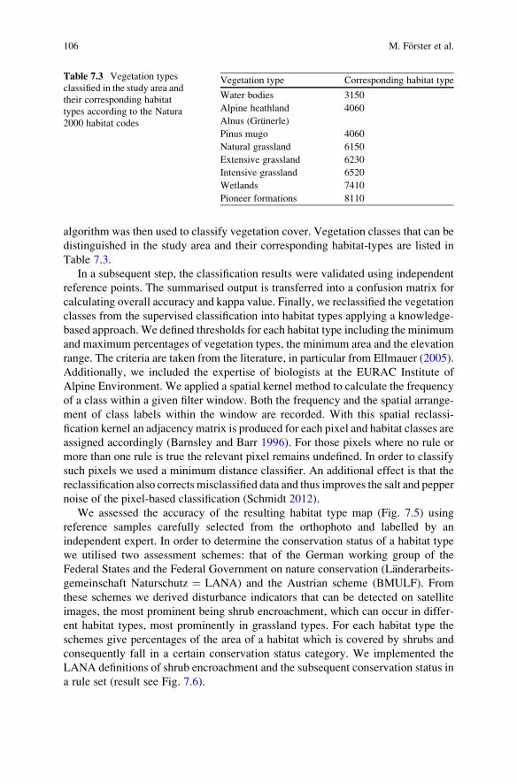
algorithm was then used to classify vegetation cover. Vegetation classes that can be

distinguished in the study area and their corresponding habitat-types are listed in

Table 7.3.

In a subsequent step, the classification results were validated using independent

reference points. The summarised output is transferred into a confusion matrix for

calculating overall accuracy and kappa value. Finally, we reclassified the vegetation

classes from the supervised classification into habitat types applying a knowledge-

based approach. We defined thresholds for each habitat type including the minimum

and maximum percentages of vegetation types, the minimum area and the elevation

range. The criteria are taken from the literature, in particular from Ellmauer (2005).

Additionally, we included the expertise of biologists at the EURAC Institute of

Alpine Environment. We applied a spatial kernel method to calculate the frequency

of a class within a given filter window. Both the frequency and the spatial arrange-

ment of class labels within the window are recorded. With this spatial reclassi-

fication kernel an adjacency matrix is produced for each pixel and habitat classes are

assigned accordingly (Barnsley and Barr 1996). For those pixels where no rule or

more than one rule is true the relevant pixel remains undefined. In order to classify

such pixels we used a minimum distance classifier. An additional effect is that the

reclassification also corrects misclassified data and thus improves the salt and pepper

noise of the pixel-based classification (Schmidt 2012).

We assessed the accuracy of the resulting habitat type map (Fig. 7.5) using

reference samples carefully selected from the orthophoto and labelled by an

independent expert. In order to determine the conservation status of a habitat type

we utilised two assessment schemes: that of the German working group of the

Federal States and the Federal Government on nature conservation (Landerarbeits-

gemeinschaft Naturschutz ¼ LANA) and the Austrian scheme (BMULF). From

these schemes we derived disturbance indicators that can be detected on satellite

images, the most prominent being shrub encroachment, which can occur in differ-

ent habitat types, most prominently in grassland types. For each habitat type the

schemes give percentages of the area of a habitat which is covered by shrubs and

consequently fall in a certain conservation status category. We implemented the

LANA definitions of shrub encroachment and the subsequent conservation status in

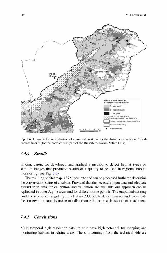
a rule set (result see Fig. 7.6).

Table 7.3 Vegetation types

classified in the study area and

their corresponding habitat

types according to the Natura

2000 habitat codes

Vegetation type Corresponding habitat type

Water bodies 3150

Alpine heathland 4060

Alnus (Grunerle)

Pinus mugo 4060

Natural grassland 6150

Extensive grassland 6230

Intensive grassland 6520

Wetlands 7410

Pioneer formations 8110


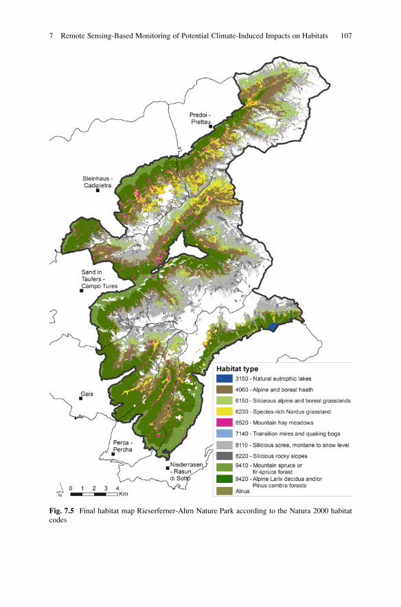
Fig. 7.5 Final habitat map Rieserferner-Ahrn Nature Park according to the Natura 2000 habitat

codes


7.4.4 Results

In conclusion, we developed and applied a method to detect habitat types on

satellite images that produced results of a quality to be used in regional habitat

monitoring (see Fig. 7.5).

The resulting habitat map is 87% accurate and can be processed further to determine

the conservation status of a habitat. Provided that the necessary input data and adequate

ground truth data for calibration and validation are available our approach can be

replicated in other Alpine areas and for different time periods. The output habitat map

could be reproduced regularly for a Natura 2000 site to detect changes and to evaluate

the conservation status bymeans of a disturbance indicator such as shrub encroachment.

7.4.5 Conclusions

Multi-temporal high resolution satellite data have high potential for mapping and

monitoring habitats in Alpine areas. The shortcomings from the technical side are

Fig. 7.6 Example for an evaluation of conservation status for the disturbance indicator “shrub

encroachment” (for the north-eastern part of the Rieserferner-Ahrn Nature Park)


mainly data gaps due to cloud cover, which is a relevant problem particularly in the

Alps. The overall accuracy of 87 % is high, taking into account the large number of

classes (12). However, while a remote sensing-based classification can hardly reach the

accuracy of a field-based survey it can compete with the widely used approach of the

photointerpretation of orthophotos. In particular the multi-temporal approach allows

classes to be separated based onphenological differences or differences inmanagement

(mowing) that cannot be separated using a mono-temporal approach like an

orthotophoto. Furthermore, the higher number of spectral bands with a better radio-

metric resolution and robustness of satellite data compared to orthophotos allow a

semi-automatic classification which saves costs and labour. Key factors for a high

quality classification result are sufficient samples in terms of amount and quality, which

should be verified in the field. Moreover, the combination of automatic classification

approaches with expert classification rules, which are based on profound knowledge of

the habitats in the region, are required for a successful application of the proposed

method. The possibility to also analyse some aspects of the conservation status of

habitats adds further value to the approach. Regarding the potential impacts of climate

change, themost obvious impact, which is a shift in vegetation zones to higher altitudes

(shrubs, treeline, glacier foreland), can be effectively monitored with remote sensing.

7.5 General Conclusion and Discussion

In this chapter the possibility of using remote sensing information for monitoring

climate-induced impacts on habitats has been demonstrated for three test cases in

the Continental, Alpine, and Pannonian biogeographic regions. Moreover, habitats

from the land-cover types forest, wetland, and Alpine environment were evaluated

to assess the feasibility of supporting the monitoring of climate change impacts.

In those test cases with a validation of the classification results, the accuracy is

higher than 80 %. Given the complexity of the target classes, this result can be

accepted as a basis for the further derivation of the conservation status of classes.

Generally, comparison with future image acquisitions for the evaluation of changes

is possible. However, these changes might have causes other than pure (and often

very gradually occurring) climate change. Variations in market prices of timber or

crops may influence usage intensity, as may the subsidy schemes of the European

Union or the changing touristic utilisation of an area. It is not possible to distinguish

anthropogenic land-use changes from those induced by climate change by means of

the methods discussed.

The results were achieved using multi-temporal RapidEye imagery. At least two

scenes per year were available for the presented studies. The advantage of utilising

several pieces of information from the phenological cycle was stated in all studies,

as well as the necessity of working with very high spatial resolution imagery

(below 10 m).


However, the compatibility and transferability of such classification results

depends on a variety of factors, including:

• comparable and high sampling intensity in space (all necessary classes equally

covered) and time (seasonally and/or according to phenological changes of the

habitat types),

• comparable sensors and spectral resolution, similar conditions for input imagery

(acquisition date/frequency, cloud cover etc.),

• comparable mapping scale or spatial precision: the minimum mapping unit (for

vector maps) or the spatial resolution (for raster maps) should be similar,

• comparable mapping accuracy, consisting of thematic accuracy (percentage of

correctly classified habitats), and spatial accuracy (habitat delineation errors),

• compatibility of habitat nomenclatures (habitat classification systems).

Summarising the experiences from the HABIT-CHANGE project, a set of key

points has to be kept in mind when considering remote sensing techniques for

habitat monitoring. In order to fulfil the goal of a focused habitat monitoring

integrating remote sensing technique, a clear vision of the outcome (objective)

has to be defined. A selection of possible questions is compiled in Table 7.4 for

consideration in further studies, for service providers as well as (or together with)

users and practitioners of the mapping or monitoring of results.

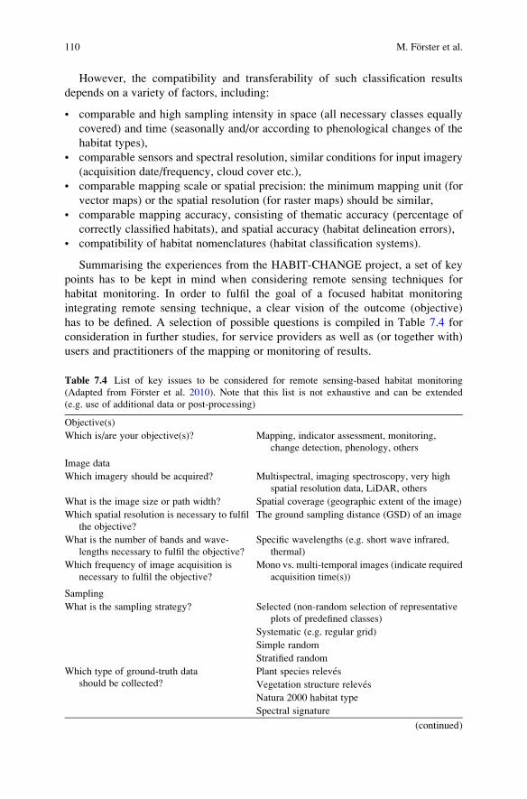
Table 7.4 List of key issues to be considered for remote sensing-based habitat monitoring

(Adapted from Forster et al. 2010). Note that this list is not exhaustive and can be extended

(e.g. use of additional data or post-processing)

Objective(s)

Which is/are your objective(s)? Mapping, indicator assessment, monitoring,

change detection, phenology, others

Image data

Which imagery should be acquired? Multispectral, imaging spectroscopy, very high

spatial resolution data, LiDAR, others

What is the image size or path width? Spatial coverage (geographic extent of the image)

Which spatial resolution is necessary to fulfil

the objective?

The ground sampling distance (GSD) of an image

What is the number of bands and wave-

lengths necessary to fulfil the objective?

Specific wavelengths (e.g. short wave infrared,

thermal)

Which frequency of image acquisition is

necessary to fulfil the objective?

Mono vs. multi-temporal images (indicate required

acquisition time(s))

Sampling

What is the sampling strategy? Selected (non-random selection of representative

plots of predefined classes)

Systematic (e.g. regular grid)

Simple random

Stratified random

Which type of ground-truth data

should be collected?

Plant species releves

Vegetation structure releves

Natura 2000 habitat type

Spectral signature

(continued)


Acknowledgements We acknowledge the DLR for the delivery of RapidEye images as part of

the RapidEye Science Archive – proposal 439. The TU Berlin thanks Ruth Sonnenschein and

Moritz Harlin for their help and fruitful discussions and Steve Kass for working on HABIT-

CHANGE project outputs 4.1.1, 4.3.7, and 4.3.9 that provided part of the basis for the descriptions

in this chapter.

Open Access This chapter is distributed under the terms of the Creative Commons Attribution

Noncommercial License, which permits any noncommercial use, distribution, and reproduction in

any medium, provided the original author(s) and source are credited.

References

Auer, I., et al. (2007). HISTALP – historical instrumental climatological surface time series of the

Greater Alpine Region. International Journal of Climatology, 27(1), 17–46. doi:10.1002/joc.1377.

Barnsley, M. J., & Barr, S. L. (1996). Inferring urban land use from satellite sensor images using

kernel-based spatial reclassification. Photogrammetric Engineering & Remote Sensing, 62(8),949–958.

Berger, M., Moreno, J., Johannessen, J. A., Levelt, P. F., & Hanssen, R. F. (2012). ESA’s sentinel

missions in support of Earth system science. Remote Sensing of Environment, 120, 84–90.Bock, M., Xofis, P., Mitchley, J., Rossner, G., & Wissen, M. (2005). Object-oriented methods for

habitat mapping at multiple scales – case studies from Northern Germany and Wye Downs,

UK. Journal for Nature Conservation, 13, 75–89.Burkhardt, R., Robisch, F., & Schroder, E. (2004). Umsetzung der FFH-Richtlinie im Wald –

Gemeinsame bundesweite Empfehlungen der Landerarbeitsgemeinschaft Naturschutz

(LANA) und der Forstchefkonferenz (FCK). Natur und Landschaft, 79, 316–323.Canty, M. J., & Nielsen, A. A. (2008). Automatic radiometric normalization of multitemporal

satellite imagery with the iteratively re-weighted MAD transformation. Remote Sensing ofEnvironment, 112, 1025–1036.

Table 7.4 (continued)

What is the season for acquisition? Month or season

Which sample size is required? No. of samples, depending e.g. on required mini-

mum samples of classification algorithm

Remote sensing derived information

Which information should be derived? Map, change, phenology, others

Which classification approaches are used? Pixel-based analysis or object-based analysis

Classification or derivation of gradual vegetation

composition

Hard classification or soft (fuzzy) classification

Supervised or unsupervised classification

Spectral or spatial

Validation

How should the result be validated? Based on dependent or independent samples

Automatic validation or visual interpretation

Pixel or polygon based

By confusion matrix or other techniques


http://dx.doi.org/10.1002/joc.1377

http://dx.doi.org/10.1002/joc.1377

Duro, D., Coops, N. C., Wulder, M. A., & Han, T. (2007). Development of a large area

biodiversity monitoring system driven by remote sensing. Progress in Physical Geography,31, 235–260.

EEA. (2009). Regional climate change and adaptation – the Alps facing the challenge of changingwater resources. Retrieved June 2012, from European Environment Agency, http://www.eea.

europa.eu/publications/alps-climate-change-and-adaptation-2009

Ellmauer, T. (2005). Entwicklung Von Kriterien, Indikatoren Und Schwellenwerten ZurBeurteilung Des Erhaltungszustandes Der Natura 2000-Schutzguter. Band 3:Lebensraumtypen des Anhangs I der Fauna-Flora-Habitat-Richtlinie. Retrieved June 2012,

from Bundesministerium f. Land- und Forstwirtschaft, Umwelt und Wasserwirtschaft und der

Umweltbundesamt GmbH, http://www.umweltbundesamt.at/fileadmin/site/umweltthemen/

naturschutz/Berichte_GEZ/Band_3_FFH-Lebensraumtypen.pdf

Forster, M., & Kleinschmit, B. (2008). Object-based classification of QuickBird data using

ancillary information for the detection of forest types and NATURA 2000 habitats. In

T. Blaschke, S. Lang, & G. Hay (Eds.), Object-based image analysis (pp. 275–290). Berlin:Springer.

Forster, M., Frick, A., Walentowski, H., & Kleinschmit, B. (2008). Approaches to utilising

Quickbird-data for the monitoring of NATURA 2000 habitats. Community Ecology, 9(2),155–168.

Forster, M., Kass, S., Neubert, M., Sienkiwicz, J., Sonnenschein, R., Wagner, I., & Zebisch,

M. (2010). Combined report on list of possible indicators and pressures, guidelines formonitoring and proposal of robust indicators for Alpine Areas, HABIT-CHANGE Output4.1.1 + 4.3.7. + 4.3.8. Retrieved March 2013, from HABIT-CHANGE, http://www.habit-

change.eu/index.php?id¼33

Gao, B. (1996). NDWI – a normalized difference water index for remote sensing of vegetation

liquid water from space. Remote Sensing of Environment, 58(3), 257–266.Haralick, R. M., Shanmugam, K., & Dinstein, I. (1973). Textural features for image classification.

IEEE transactions on systems. Man and Cybernetics, 3(6), 620–621.Karatzoglou, A., Meyer, D., & Hornik, K. (2005). Support vector machines in R. Retrieved July

20, 2012, form 21. Department of Statistics and Mathematics, WU Vienna University of

Economics and Business, http://epub.wu.ac.at/1500/

Lang, S., & Langanke, T. (2005). Multiscale GIS tools for site management. Journal for NatureConservation, 13, 185–196.

Lengyel, S., Deri, E., Varga, Z., Horvath, R., Tothmeresz, B., Henry, P. Y., Kobler, A., Kutnar, L.,

Babij, V., Seliskar, A., Christia, C., Papastergiadou, E., Gruber, B., & Henle, K. (2008).

Habitat monitoring in Europe: A description of current practices. Biodiversity and Conserva-tion, 17, 3327–3339.

Papastergiadou, E. S., Retalis, A., Kalliris, P., & Georgiadis, T. (2007). Land use changes and

associated environmental impacts on the mediterranean shallow lake Stymfalia, Greece.

Hydrobiologia, 584, 361–372.Polastre, J., Szewczyk, R., Mainwaring, A., Culler, D., & Anderson, J. (2004). Analysis of wireless

sensor networks for habitat monitoring. In C. S. Raghavendra, K. M. Sivalingam, & T. Znati

(Eds.), Wireless sensor networks (pp. 399–423). New York: Springer US.

Rocchini, D., Foody, G., Nagendra, H., Ricotta, C., Anand, M., He, K., Amici, V., Kleinschmit, B.,

Forster, M., Schmidtlein, S., Feilhauer, H., Ghisla, A., Metz, M., & Neteler, M. (2013).

Uncertainty in ecosystem mapping by remote sensing. Computers and Geoscience, 50,128–135.

Schmidt, A. (2012). Conversion of a remote sensed vegetation classification to a habitat map –Comparing a spatial kernel and an object-based approach (Unpublished diploma thesis).

Schuster, C., Forster, M., & Kleinschmit, B. (2012). Testing the red edge channel for improving

land-use classifications based on high-resolution multi-spectral satellite data. InternationalJournal of Remote Sensing, 33, 5583–5599.


http://www.eea.europa.eu/publications/alps-climate-change-and-adaptation-2009

http://www.eea.europa.eu/publications/alps-climate-change-and-adaptation-2009

http://www.umweltbundesamt.at/fileadmin/site/umweltthemen/naturschutz/Berichte_GEZ/Band_3_FFH-Lebensraumtypen.pdf

http://www.umweltbundesamt.at/fileadmin/site/umweltthemen/naturschutz/Berichte_GEZ/Band_3_FFH-Lebensraumtypen.pdf

http://www.habit-change.eu/index.php?id=33



http://epub.wu.ac.at/1500/

Soja, G., Zuger, J., Knoflacher, M., Kinner, P., & Soja, A. (2013). Climate impacts on water

balance of a shallow steppe lake in Eastern Austria (Lake Neusiedl). Journal of Hydrology,480, 115–124.

Toutin, T. (2003). Error tracking in IKONOS geometric processing using a 3D parametric model.

Photogrammetric Engineering & Remote Sensing, 69(1), 43–51.Tucker, C. J. (1979). Red and photographic infrared linear combinations for monitoring vegeta-

tion. Remote Sensing of Environment, 8, 127–150.Turner, W., Spector, S., Gardiner, N., Fladeland, M., Sterling, E., & Steininger, M. (2003). Remote

sensing for biodiversity science and conservation. Trends in Ecology and Evolution, 18,306–314.

Vehmas, M., Eerikainen, K., Peuhkurinen, J., Packalen, P., & Maltamo, M. (2009). Identification

of boreal forest stands with high herbaceous plant diversity using airborne laser scanning.

Forest Ecology and Management, 257, 46–53.Wulder, M. A., White, J. C., Masek, J. G., Dwyer, J., & Roy, D. P. (2011). Continuity of Landsat

observations: Short term considerations. Remote Sensing of Environment, 115, 747–751.Zebisch, M., Kass, S., & Tasser, E. (2010). Potential pressures + indicators for NATURA 2000

reporting in Alpine Habitats – Nature Park Rieserferner Ahrn, HABIT-CHANGE Output4.1.4 + 4.1.5. Retrieved July 2012, from HABIT-CHANGE, http://www.habit-change.eu/

index.php?id¼33





Documents

Chapter 7 Remote Sensing-Based Monitoring of Potential Climate-Induced Impacts on Habitats · 2017-08-27 · Remote Sensing-Based Monitoring of Potential Climate-Induced Impacts on