Embed Size (px)
Citation preview

Chapter 7
Sediment transport model
7.1 Introduction
This chapter describes the sediment transport model implemented in COHE-RENS. There are six sections. In the first one, a discussion is given of phys-ical parameters and processes (bed shear stress, molecular viscosity, waves)which are of importance for the sediment and the influence of sedimentson the physics through density gradients. In the next section a descriptionis given of the basic sediment parameters (Shield parameter, fall velocity,critical shear stress), related to sediment transport. This is followed by anoverview of the bed and total load equations available in COHERENS. Then,the suspended sediment transport module is presented. Finally, numericaltechniques, specific for the sediment module, are described.
7.2 Physical aspects
7.2.1 Bed shear stresses
The bed shear stress is considered as the physical parameter which has thelargest impact on sediment transport, since it controls how much of the se-diment in the bed layer becomes suspended in the water column. In thephysical part of COHERENS, bottom stresses are calculated using either alinear or a quadratic friction law (see Section 4.9). In the sediment transportmodule, however, a quadratic friction law is always taken, as given by equa-tion (4.340) in 3-D or (4.341) in 2-D mode. The magnitude of the bottomstress can then be written as
τb = ρu2∗b = ρCdbu2b or τb = ρu2∗b = ρCdb|u|2 (7.1)
311

312 CHAPTER 7. SEDIMENT TRANSPORT MODEL
for the 3-D, respectively 2-D case. In the equations, u∗b is the wall shear(friction) velocity1, ub the bottom current, |u| the magnitude of the depthmean current and Cdb the bottom drag coefficient given by
Cdb =[ κ
ln(zb/z0
)]2 or Cdb =[ κ
ln(H/z0)− 1
)]2 (7.2)
for the 3-D, respectively 2-D case. Here, κ is the Von Karman constant, zbheight of the first velocity node above the sea bed, z0 the roughness heightand H the total water depth.
In the discussions of the load formulae, given in the sections below, otherformulations, obtained from engineering practice, are mentioned and givenhere for completeness:
Cdb =g
C2Chezy (7.3)
Cdb =gM2
H1/3Manning (7.4)
Cdb =g
[18 log (2H/5z0)]2 White-Colebrook (7.5)
The coefficients C and M are denoted as the Chezy, respectively Manningcoefficients.
In case of a rough bed, the roughness length z0 can be calculated usingthe following relation:
z0 = 0.11ν
u∗+kb30≈ kb
30(7.6)
Here, kb is the roughness height from Nikuradse, ν the kinematic viscosityand u∗ the friction velocity.
Different kinds of roughness height are considered:
• Physical or “form” roughness kb representing the heights of the elementscomposing the bottom roughness. The corresponding physical bottomstress is used as boundary condition for the momentum flux at thebottom.
• “Skin” roughness ks usually related to the median particle size. Skinstress is used in the sediment module to calculate the amount of sedi-ment material resuspended from the sea bed, once the stress exceeds acritical value (see below).
1Since the friction velocity always refers to the bottom in this chapter, the subscript bwill be omitted in the following.

7.2. PHYSICAL ASPECTS 313
• The main effect of surface waves on the bottom stress is a significantincrease of both the form and skin roughness heights. The new rough-ness height, denoted as ka, is obtained from formulae for current-waveinteraction theories. The formulations are currently not implementedin COHERENS, but foreseen in a future version of the code.
COHERENS provides different options for the selection of the skin bottomroughness. Either the form roughness, as used by the hydrodynamics, istaken as the skin roughess, or a constant user-defined value is supplied orspatially non-uniform values are provided by the user. A further advantage isthat the user can calibrate the sediment transport rates in this way withoutchanging the hydrodynamics. Note that, in the current version of the code,no formulation has been implemented for the skin roughness as function ofmedian size, although ks can always be externally supplied by the user.
7.2.2 Wave effects
Although surface waves effects have not been implemented in the physicalpart of the code, the bottom stresses used in the load formulae, discussedbelow, take account of both currents and waves. A summary of the appliedmethods is given in this subsection.
The wave field is supplied externally by a significant wave height Hs,a wave period Tw and a wave direction φw. The wave amplitude Aw andfrequency are defined by
Aw = Hs/2 , ωw = 2π/Tw (7.7)
The near-bottom wave orbital velocity determined from linear wave theoryis given by
Uw =Awωw
sinh kwH(7.8)
with the wavenumber kw obtained from the dispersion relation
ω2w = gkw tanh kwH (7.9)
The latter equation is solved for kw using the approximate formula of Hunt(1979)
kw = ωw
√f(α)
gH(7.10)
with
f(α) = α +(1.0 + 0.652α + 0.466422α2 + 0.0864α4 + 0.0675α5
)−1(7.11)

314 CHAPTER 7. SEDIMENT TRANSPORT MODEL
and
α =ω2wH
g(7.12)
With this option, it is assumed that the near bed wave period is equal to themean wave period, such that the near bed wave excursion amplitude can bewritten as
Ab =Uwωw
(7.13)
The combined effect of currents and waves on the bed shear stress is calcu-lated using the method described in Soulsby (1997). Two types of bottomstress are defined
• The mean value over the wave cycle which should be used for currents
τm = τc
[1 + 1.2
(τw
τc + τw
)3.2]
(7.14)
where τc is the bottom stress for currents alone as given by (7.1)–(7.2).
• The maximum value during the wave cycle used in the criterion forresuspension
τmax =√τ 2m + τ 2w + 2τmτw cosφw (7.15)
where the wave bottom stress is defined by
τw =1
2fwU
2w (7.16)
Two formulations are used for the wave friction
• Swart (1974)
fw = 0.3 for Ab/kb ≤ 1.57
fw = 0.00251 exp(
5.21(Ab/kb)−0.19
)for Ab/kb > 1.57
(7.17)
• Soulsby et al. (1993)
fw = 0.237(Ab/kb)−0.52 (7.18)

7.2. PHYSICAL ASPECTS 315
7.2.3 Density effects
7.2.3.1 Equation of state
The fluid density is an important parameter for calculating settling velocitiesand entrainment rates in sediment transport. The equation of state that isused to calculate the fluid density as function of the water temperature andsalinity is discussed in Section 4.2.3. When sediment is present, an additionaleffect is present in the equation of state
ρ = (1−N∑n=1
cn)ρw +N∑n=1
cnρs,n (7.19)
Here ρ is the density of the mixture, ρw the density of the fluid (including theeffects of temperature, pressure and salinity), cn the volume concentrationof fraction n, N the number of sediment fractions and ρs,n the particle den-sity for sediment fraction n. A stable vertical sediment stratification leads todamping of turbulence and affects the settling velocity of the sediment. How-ever, care must be taken when applying this in combination with hinderedsettling (Section 7.3.3.2), because hindered settling models already accountfor the increased buoyancy of the mixture. Thus using a changed equationof state in combination with hindered settling will result in too low settlingvelocities.
7.2.3.2 Density stratification
To a large extent, the two-way coupling effects between flow and sedimenttransport are due to density stratification effects. Villaret & Trowbridge(1991) showed that the effects of the stratification from suspended sedimentare very similar (even with the same coefficients) to the ones produced bytemperature and salinity gradients. This means that the effects of sediment-turbulence interaction in COHERENS can be implemented within the existingturbulence models in the same way as T and S.
The (squared) buoyancy frequency in the presence of vertical sedimentstratification becomes:
N2 = N2w − g
N∑n=1
βc,n∂cn∂z
(7.20)
where N2w is the value in the absence of sediment stratification, as given by
(4.130) and βc,n, the expansion coefficient for sediment fraction n, which is

316 CHAPTER 7. SEDIMENT TRANSPORT MODEL
calculated from the density of each sediment fraction ρs,n using:
βc,n =1
ρ
∂ρ
∂cn=ρs,n − ρw
ρ(7.21)
The baroclinic component of the horizontal pressure gradient contains anadditional term due to horizontal sediment stratification. Equation (5.223)now becomes
− ∂q
∂xi' g
∫ ζ
z
(βT∂T
∂xi− βS
∂S
∂xi−
N∑n=1
βc,n∂c
∂xi
)dz′ (7.22)
In transformed coordinates the following term is added to right hand side of(5.224) for each fraction n:
F c,ni = −g
∫ ζ
z
βc,n
(∂cn∂xi
∣∣∣s− ∂cn∂z′
∂z′
∂xi
∣∣∣s
)dz′ (7.23)
The numerical methods, described in Section 5.3.13 for discretising the baro-clinic gradient are easily extended to include sediment stratification.
7.2.4 Kinematic viscosity
The kinematic viscosity ν is an important parameter that has a significantinfluence on the settling velocity and the critical bed stress. Its value can beselected in COHERENS either as a user-defined constant or as a temperaturedependent value using the ITTC (1978) equation for sea water
ν = 10−6[1.7688 +
(0.659.10−3 (T − 1)− 0.05076
)(T − 1)
](7.24)
Here T is the water temperature in 0C and ν is given in m2/s.
Implementation
The following switches are available:
iopt sed tau Selects type of roughness height zs used for sediment transport
1: set equal to the form roughness used in the hydrodynamics
2: user-defined uniform value
3: spatially non-uniform value supplied by the user
iopt waves Disables/enables wave effects and selects type of input data wavedata, for use in the sediment transport models.

7.3. SEDIMENT PROPERTIES 317
0: wave effects disabled
1: waves enabled with input of wave height, period and direction
2: waves enabled with input of wave height, period, velocity, excursionand direction
iopt sed dens Disables (0) or enables (1) effects of sediments in the equationof state and density stratification.
iopt kinvisc Selects type of kinematic viscosity.
0: user-selected uniform value
1: from the ITTC (1978) equation
7.3 Sediment properties
7.3.1 Introduction
Sediment concentrations can be represented either as a volumetric concen-tration c in units of m3/m3 or as a mass concentration cmass in kg/m3.Thetwo forms are related by
cmass = ρsc (7.25)
The volumetric form is taken in COHERENS, which is considered as morephysically meanigfull, especially in processes as hindered settling.
A dimensional analysis by Yalin (1977) shows that the sediment transportcan be expressed by a number of dimensionless parameters:
Re∗ =u∗d
ν(7.26)
θ =ρu2∗
(ρs − ρ)gd(7.27)
s =ρsρ
(7.28)
d∗ = d[(s− 1)
g
ν2
]1/3(7.29)
Φ =q√
(s− 1)gd3(7.30)
where d is the particle diameter, Re∗ the particle Reynolds number, θ thedimensionless shear stress or Shields parameter (Shields, 1936), s the relativedensity, d∗ the dimensionless particle diameter and q the sediment load perunit width (in m2/s).

318 CHAPTER 7. SEDIMENT TRANSPORT MODEL
These non-dimensional diameters are often used to describe sedimentproperties, such as critical shear stresses or settling velocities, which arediscussed below.
7.3.2 Critical shear stress
In many transport relations, a critical shear stress is required, which is thevalue of the bed shear stress at which the sediment particles start to move(the threshold of motion). The value of the bed shear stress is in engineeringpractice obtained from the Shields curve, which relates the non-dimensionalcritical shear stress θcr to the particle Reynolds number Re∗.
For numerical models, some fits to these curves are made, expressing θcras a function of d∗ rather than Re∗, in order to avoid the iteration processnecessary for the determination of the threshold of motion in the originalcurve obtained by Shields (1936), as both θ and Re∗ are a function of u∗.Brownlie (1981) obtained the following relation from a fit through the data:
θcr = 0.22d−0.9∗ + 0.06.10(−7.7d−0.9∗ ) (7.31)
An alternative form, also obtained by fitting of the Shields curve, is pro-posed by Soulsby & Whitehouse (1997)
θcr =0.3
1 + 1.2d∗+ 0.055
(1− e−0.02d∗
)(7.32)
Another equation, available in COHERENS from Wu et al. (2000), is toassume a constant critical Shields stress
θcr = 0.03 (7.33)
This equation should only be used in combination with the bed load andtotal load equations from Wu et al. (2000). In COHERENS, the critical shearstress is calculated for each fraction separately at each horizontal location,using the local values of the kinematic viscosity and the mixture density.
The sediment transport model in COHERENS has an option available forthe user to manually set the critical shear stress. The user can either setthe critical shear stress to a uniform value throughout the whole domain,or to a spatially varying value. Be aware that the value given should bethe kinematic critical shear stress defined as the square of the critical shearvelocity u2∗,cr = τcr/ρ.

7.3. SEDIMENT PROPERTIES 319
7.3.2.1 Hiding and exposure
A hiding and exposure factor can be implemented for the critical shear stressτcr or the critical Shields parameter θcr to account for the change in sedimenttransport when different fractions are present. In general, the correctionfactor will increase the critical value for the smaller, hidden fractions andwill reduce the critical threshold for motion for the coarser, exposed, frac-tions. Several formulations can be found in literature, usually as a functionξ(dn/d50).
Two methods are available in COHERENS for hiding and exposure. Thefirst one uses the formulation of Wu et al. (2000) based upon a stochasticrelation between size and gradation of bed materials and the hidden andexposed probabilities. The probability of particles dm in front of particles dncan be assumed to be the fraction of particles dm in the bed material, pbm.The total hidden and exposed probabilities of particles dn can be describedby:
phn =N∑m=1
pbmdm
dn + dm(7.34)
pen =N∑m=1
pbmdn
dn + dm(7.35)
and phn + pen = 1. The hiding/exposure factor is then defined by:
ξn =
(penphn
)m=
(1− phnphn
)m(7.36)
where m is an empirical parameter which Wu et al. (2000) determined asm = −0.6 in their study.
Alternatively, hiding and exposure can be calculated with the equationof Ashida & Michiue (1972), which is an adapted form of Egiazaroff (1965)
ξn =
{0.8429d50
dnif d50
dn< 0.38889[
log 19log 19+log(dn/d50)
]2if d50
dn≥ 0.38889
(7.37)
where d50 is the median grain size diameter, which, in case multiple sizefractions are present, means that particles with sizes less than d50 accountfor 50% of the total mass.
320 CHAPTER 7. SEDIMENT TRANSPORT MODEL
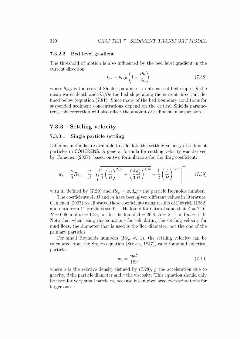
7.3.2.2 Bed level gradient
The threshold of motion is also influenced by the bed level gradient in thecurrent direction
θcr = θcr,0
(1− ∂h
∂c
)(7.38)
where θcr,0 is the critical Shields parameter in absence of bed slopes, h themean water depth and ∂h/∂c the bed slope along the current direction, de-fined below (equation (7.81). Since many of the bed boundary conditions forsuspended sediment concentrations depend on the critical Shields parame-ters, this correction will also affect the amount of sediment in suspension.
7.3.3 Settling velocity
7.3.3.1 Single particle settling
Different methods are available to calculate the settling velocity of sedimentparticles in COHERENS. A general formula for settling velocity was derivedby Camenen (2007), based on two formulations for the drag coefficient:
ws =ν
dRep =
ν
d
√1
4
(A
B
)2/m
+
(4
3
d3∗B
)1/m
− 1
2
(A
B
)1/mm (7.39)
with d∗ defined by (7.29) and Rep = wsdp/ν the particle Reynolds number.The coefficients A, B and m have been given different values in literature.
Camenen (2007) recalibrated these coefficients using results of Dietrich (1982)and data from 11 previous studies. He found for natural sand that A = 24.6,B = 0.96 and m = 1.53, for flocs he found A = 26.8, B = 2.11 and m = 1.19.Note that when using this equations for calculating the settling velocity formud flocs, the diameter that is used is the floc diameter, not the one of theprimary particles.
For small Reynolds numbers (Rep � 1), the settling velocity can becalculated from the Stokes equation (Stokes, 1847), valid for small sphericalparticles
ws =sgd2
18ν(7.40)
where s is the relative density defined by (7.28), g the acceleration due togravity, d the particle diameter and ν the viscosity. This equation should onlybe used for very small particles, because it can give large overestimations forlarger ones.

7.3. SEDIMENT PROPERTIES 321
The following formulation is recommended by Soulsby (1997) for naturalsands
ws =ν
d
[√10.362 + 1.049d3∗ − 10.36
](7.41)
Another equation for the settling velocity, available in COHERENS is theone by Zhang & Xie (1993)
ws =
√(13.95
ν
d
)2+ 1.09 (s− 1) gd− 13.95
ν
d(7.42)
7.3.3.2 Hindered settling
In case of high concentrations (mass concentrations larger than 3 g/l) thesettling of particles is not only influenced by the surrounding fluid and theweight and shape of the particles, but also by the other particles in suspen-sion. The settling of the particles is reduced by a number of processes, e.g.return flow, particle collisions, changed mixture viscosity, buoyancy due toincreased mixture density and wake formation.
For sand, hindered settling can be calculated with the equation of Richard-son & Zaki (1954). They described the settling velocity in high sedimentconcentrations as a function of the sediment concentration, Rep and undis-turbed settling velocity ws,0 (i.e. the one of a single particle without beingdisturbed):
ws = ws,0 (1− c)n (7.43)
In this equation, n is a user-defined constant. Note that this formula isnot advisable for cohesive sediments because it does not take into accountthe maximum sediment concentration (i.e. the settling velocity should reduceto zero at the maximum packing concentration cmax). This is not a severedisadvantage, because in most practical applications, the concentrations arenot so high, except close to the sea bed. Note that some hindered settlingeffects are already calculated when the fluid density depends on the sedimentconcentrations, and that this equations are only valid when a net depositionoccurs (Breugem, 2012). Therefore, it is recommended not to use hinderedsettling in that case.
Winterwerp & van Kesteren (2004) introduced a different formula for mud
ws = ws,0(1− cf )(1− c)
1 + 2.5cf(7.44)
Here ws,0 is the settling velocity of a single mud-floc, cf = c/cgel, cgel is thegelling concentration (the mass concentration at which the mud flocs form a

322 CHAPTER 7. SEDIMENT TRANSPORT MODEL
space filling network), which can be calculated with
cgel = ρsdpdf
3−nf(7.45)
The parameters needed to calculate the gelling concentration (nf and df )are difficult to determine. Therefore, the user must provide a value for cgel,which should be obtained from measurements.
7.3.3.3 Influence of flocculation
In COHERENS, the influence of turbulence and sediment concentration onthe flocculation of mud flocs can be simulated. The effect of salinity is notconsidered. For simulating the influence of turbulence the empirical modelby Van Leussen (1994) is used for the fall velocity of settling flocs
wsws,r
=1 + aG
1 + bG2(7.46)
Here ws,r is a reference velocity, G the shear rate, defined as G =√ε/ν
and a, b empirical constants. In order to estimate the shear rate if theturbulent dissipation ε is not known (e.g. when an algebraic turbulencemodel is used), G can be obtained assuming equilibrium between productionand dissipation of turbulent kinetic energy (4.204) which gives 2
G =
√νTM2 − λTN2
ν(7.47)
where νT , λT are the turbulent diffusion coefficients for respectively mo-mentum and density and M , N the shear and buoyancy frequencies (seeSection 4.4 for details).
A similar empirical approach to flocculation, which considers the influenceof the sediment concentration is given in Van Rijn (2007b)
wsws,r
=[4 + log10
(2c/cgel
)]α= φfloc (7.48)
with 1≤ φfloc ≤10 and α a user-defined constant with a minimum of 0 anda maximum of 3, whose default value in COHERENS was obtained fromcalibration of flocculation data in the Scheldt and harbour of Zeebrugge. Note
2Note that G has a different meaning than in Section 4.4 where it represents thebuoyancy term in the turbulent energy equation.

7.3. SEDIMENT PROPERTIES 323
that Van Rijn (2007b) suggests α = dsand/d50− 1, with dsand the diameter ofthe transition from sand to silt (62 µm).
It is also possible to combine the effects of these two models in COHE-RENS. In this case, the settling velocity is multipled by the two correctionsfactors on the right of (7.46) and (7.48).
Implementation
The methods in this section are selected with the following switches
iopt sed taucr Selects type of method for the critical shear stress
1: user-defined value for each fraction
2: Brownlie (1981) equation (7.31)
3: Soulsby & Whitehouse (1997) equation (7.32)
4: Wu et al. (2000) equation (7.33)
iopt sed hiding Type of hiding/exposure factor for the critical shear stress
0: hiding disabled
1: Wu et al. (2000) equation (7.36)
2: Ashida & Michiue (1972) equation (7.37)
iopt sed ws Type of method for the settling velocity
1: user-defined value for each fraction
2: Camenen (2007) formulation (7.39) for sand
3: Camenen (2007) formulation (7.39) for mud
4: Stokes formula (7.40)
5: Soulsby (1997) formula (7.41)
6: Zhang & Xie (1993) equation (7.42)
iopt sed hindset Formulation for hindered settling
0: hindered settling disabled
1: Richardson & Zaki (1954) equation (7.43)
2: Winterwerp & van Kesteren (2004) formula (7.44)
iopt sed floc Type of flocculation factor for the settling velocity
0: flocculation effect disabled
1: Van Leussen (1994) equation (7.46)
2: Van Rijn (2007b) equation (7.48)
3: combination of the two previous methods

324 CHAPTER 7. SEDIMENT TRANSPORT MODEL
7.4 Bed load
7.4.1 Introduction
In this section an overview of available models for bed load transport is given.These models are applicable to non-cohesive sediment transport and can beused in combination with suspended transport equations except for the totalload models, discussed in Section 7.5 below. Bed load is active in the near-bed layer with thickness taken often as zsb ≈ 2d. Both states are coupled bythe reference concentration ca, which is defined as the sediment concentrationin the near-bed layer.
Bed load is usually expressed as the intensity of solid discharge, whichcan be written in non-dimensional form (see also equation (7.30)):
Φb =qb√
(s− 1)gd3(7.49)
where qb is the bed load solid discharge per unit width in m2/s.The Meyer-Peter-Muller and the Einstein equations are two examples
using dimensionless parameters for relating solid discharge to the shear stressat the bed. However, the solid discharge rates of bed load, suspended loadand total load in this numerical model are given as the dimensional quantitiesexpressing the volumetric discharge per unit flow-perpendicular width (inm2/s).
The bed load transport is assumed to occur below the roughness level z0,i.e. below the lowest σ-layer. The bed load transport vector is decomposedin the same manner as the horizontal velocity vector. The bed load transportmagnitude is computed as the vector sum of transport components along theξ1 and ξ2 directions, assuming local orthogonality of the computational grid:
qb = (qb1, qb2) (7.50)
The ξ1 and ξ2 components are computed at the U-, respectively V-nodes gridpoints. This avoids that interpolations of the velocity components to e.g. theC-points need to be taken prior to the determination of sediment transportrates.
7.4.1.1 Transport of different sediment size classes
COHERENS permits to simulate the transport of different sediment classes(n = 1, . . . , nf ), each having a fraction fn present in the bed sediments.Each sediment class will experience hiding or exposure due to the presenceof grains of different size in its vicinity. The effect is introduced in the model

7.4. BED LOAD 325
by means of a hiding/exposure factor (see Section 7.3.2.1 for more detailedinformation).
7.4.1.2 Applicability of transport models
Every sediment transport formulation has been developed and calibrated un-der controlled conditions where a certain range of parameters such as particlediameters has been covered. The formulations are therefore only valid un-der the conditions covered by the experiments that lead to the formula withtuned parameters. The model user should take these limitations into accountwhen applying a formula. The range of applicability of a number of transportformula has been given in table 7.1.
Table 7.1: Overview of applicability of sediment transport formula, i.e. con-ditions of the measurements used as calibration data (if available).
d [mm] dx, for non-uniform granulate
Meyer-Peter & Muller (1948) 3.1-28.6 d50Ackers & White (1973) a 0.04-4.0 d35Engelund & Fredsøe (1976) 0.19-0.93 d50Van Rijn (1993) 0.2-2.0 d50Wu et al. (2000) 0.06-32 graded
aDiscussed in Section 7.5 below
7.4.2 Meyer-Peter and Mueller (1948)
The formula of Meyer-Peter & Muller (1948) relates the Shields parameter θnto the intensity of solid discharge Φn for sediment class n, with the followingformula
Φn = 8fn(ξMθn − ξnθcr,n)3/2 (7.51)
Here, θcr,n is the critical dimensionless shear stress, the threshold abovewhich motion of the sediment particles begins, and ξn the hiding or exposurefactor for sediment class n. The parameter ξM is a roughness parameterexpressing the relative importance of bed forms in the total roughness, equalto 1 in absence of bed forms and 1 > ξM > 0.35 if bed forms are present:
ξM =
(M ′
M
)3/2
(7.52)

326 CHAPTER 7. SEDIMENT TRANSPORT MODEL
where M is Manning’s roughness parameter for the total roughness and M ′
the Manning roughness for granulates only [m−1/3s]. In the current versionof the model, separate bed form roughness has not yet been implemented,so that the factor ξM is always set to 1. However, when the user specifiesthe friction factor to be used for sediment transport calculations as the skinfriction roughness, an equivalent result is obtained as bed load transport isassumed to be independent of form drag in this model (see Section 7.2.1).
It is important to mention under which circumstances a sediment trans-port relation has been developed, and hence its validity range. The Meyer-Peter-Muller formula (e.g.) is applicable for large sediment grain sizes, i.e.d > 3.1 mm. See also table 7.1.
7.4.3 Engelund and Fredsøe (1976)
From an equilibrium of agitating and stabilizing forces, a dimensionless ex-pression was found for the bed load transport. The agitating forces consistof drag and lift, while the stabilising forces are reduced gravity and friction.The agitating forces can be expressed as a drag force:
FD =cl2ρU2
p
πd2
4(7.53)
The coefficient cl can be seen as a correction of the drag force for lifting, Upis the particle migration velocity.
The friction force experienced by the particles can be expressed as:
Ff = ρg(s− 1)πd3
6β (7.54)
where β is a dynamic friction coefficient.When both forces are in equilibrium the following is obtained:
Upu∗
= α[1−
√θ0/θ
](7.55)
in which θ0 = 4β/3α2c and α = 9 represents the ratio of the current, takenat two grain sizes from to the bottom, to the friction velocity.
Using measurements to determine the parameters, and using the numberof particles in the bed load layer per unit area, based on a particle probabilityp, the following bed load transport equation is found:
qb = 9.3π
6dpu∗
[1− 0.7
√θcr/θ
](7.56)

7.4. BED LOAD 327
or, in non-dimensional form:
Φ = 5p(√θ − 0.7
√θcr) (7.57)
In the case of fractional transport this becomes:
Φn = 5pfn(√θ − 0.7
√ξnθcr,n) (7.58)
The probability of mobility of a sediment grain p is expressed as follows:
p =
[1 +
( πfd/6θ − θcr
)4]−1/4(7.59)
with θ > θcr and fd the dynamic friction coefficient of a grain, assumed tobe equal to 0.51.
This relation was proven to be accurate for fine to medium sands, withexperiments using sand with diameters of 190, 270 and 930 µm.
7.4.4 Van Rijn (1984b)
Van Rijn (1984b) used the method of Bagnold (1954) to determine the bedload sediment transport. Bed load transport is here dominated by particlesaltation with height δb causing a bed load concentration cb with particlesmoving at a velocity equal to Up. Unlike in the formulation of Engelund &Fredsøe (1976), only drag and lift forces as well as reduced weight are takeninto account. The bed load transport was then assumed to be qb = Upδbcb.
The bed load transport by currents for particles with diameter in therange of 200 to 2000 µm is determined by:
Φn = 0.053fnT2.1n d−0.3∗ (7.60)
where
Tn = max
(τbτcr,n
− 1, 0
)(7.61)
The implementation of this formula also allows for the computation oftransport of different size classes n with different bed fractions fn.
7.4.5 Wu et al. (2000)
This equation is specially recommended for the calculation of graded sedi-ment, because in its determination, the different fractions were explicitlytaken into account.

328 CHAPTER 7. SEDIMENT TRANSPORT MODEL
The following steps are taken to calculate the suspended load and bedload transport. Firstly, the settling velocity of fraction n is calculated withformula (7.42) from Zhang & Xie (1993). Then the hiding and exposurefactors phn and pen are computed as defined in Section 7.3.2.1.
The critical shear stress (taking into account hiding and exposure) forfraction n is calculated:
τcr,n = 0.03(ρs − ρ)gdn
(phnpen
)0.6
(7.62)
The bed load sediment transport is then determined with:
Φb,n = 0.0053fn
[max
(τbτcr,n
− 1, 0
)]2.2(7.63)
whereby the hiding/exposure factor ξn for sediment class n, is alwayscalculated with the method of Wu et al. (2000), as given by (7.34)–(7.36).
7.4.6 Soulsby (1997)
The bed load transport equation by Soulsby (1997) is an approximationobtained by integrating the bed load equation over one wave period with asinusoidal oscillatory component. The components Φbc and Φbn along thedirections parallel, respectively perpendicular to the current direction areobtained as follows
Φbc,1 = 12√θm(θm − θcr,n)
Φbc,2 = 12(0.95 + 0.19 cos 2φw)√θwθm
Φbc = fn max[Φbc,1,Φbc,2]
Φbn = fn12(0.19θmθ
2w sin 2φw)
θ1.5w + 1.5θ1.5m(7.64)
and Φbc = Φbn = 0 if θmax ≤ θcr. θm is the value of θ averaged over the wavecycle, θw, is the amplitude of the oscillatory component of θ and φ the anglebetween current and wave propagation direction. The maximal value of theShields parameter θmax over the wave cycle is calculated as follows
θmax =√θ2m + θ2w + 2θmθw cos2 φw (7.65)
The wave-averaged Shields parameter θ is determined by the relationshipfrom Soulsby (1995):
θm = θc
[1 + 1.2
(θw
θc + θw
)3.2]
(7.66)

7.4. BED LOAD 329
where θc is the current related Shields parameter. Note that (7.66) and (7.65)are the dimensionless versions of (7.14)–(7.15).
From the equations it can be seen that when the wave direction is per-pendicular or along the current direction, the component at right angle tothe current direction is zero. No wave asymmetry is taken into account.
In the absence of waves, one has Φbc,2 = Φbn = 0 so that
Φb = Φc = 12√θmax (θ − θcr,n, 0) (7.67)
The formula is implemented on the numerical grid by computing Φbc andΦbn both at U- and V-velocity points, after which they are projected on theξ1 and ξ2 grid orientation. More details are given in Section 7.7.2.
7.4.7 Van Rijn (2007a)
In an unpublished paper by Van Rijn (2003) an approximative bed loadtransport formula was determined in combination with time-integrated for-mulations for wave-related and current-related suspended sediment trans-port. In this sediment transport code, it was decided to combine the mo-dified full equation (instantaneous transport integrated over a wave period)by Van Rijn (1993) with the approximative formulations for suspended load(see Section 7.5), resulting in the total sediment transport. The instaneousbed load formula is the one given in Van Rijn (1993) but with modificationson a calibration factor and the exponent η
qb = fnγρsd50d−0.3∗ (τb,cw/ρ)1/2[(τb,cw − τb,cr)/τb,cr]η (7.68)
in which
τb,cw = 0.5ρwfcw(Uδ,cw)2 (7.69)
fcw = αβfc + (1− α)fw (7.70)
fc = 2[ κ
ln(15H/ks)
]2(7.71)
fw = 0.00251 exp(
5.21(Aw/ks)−0.19
)(7.72)
and fw given by (7.18).
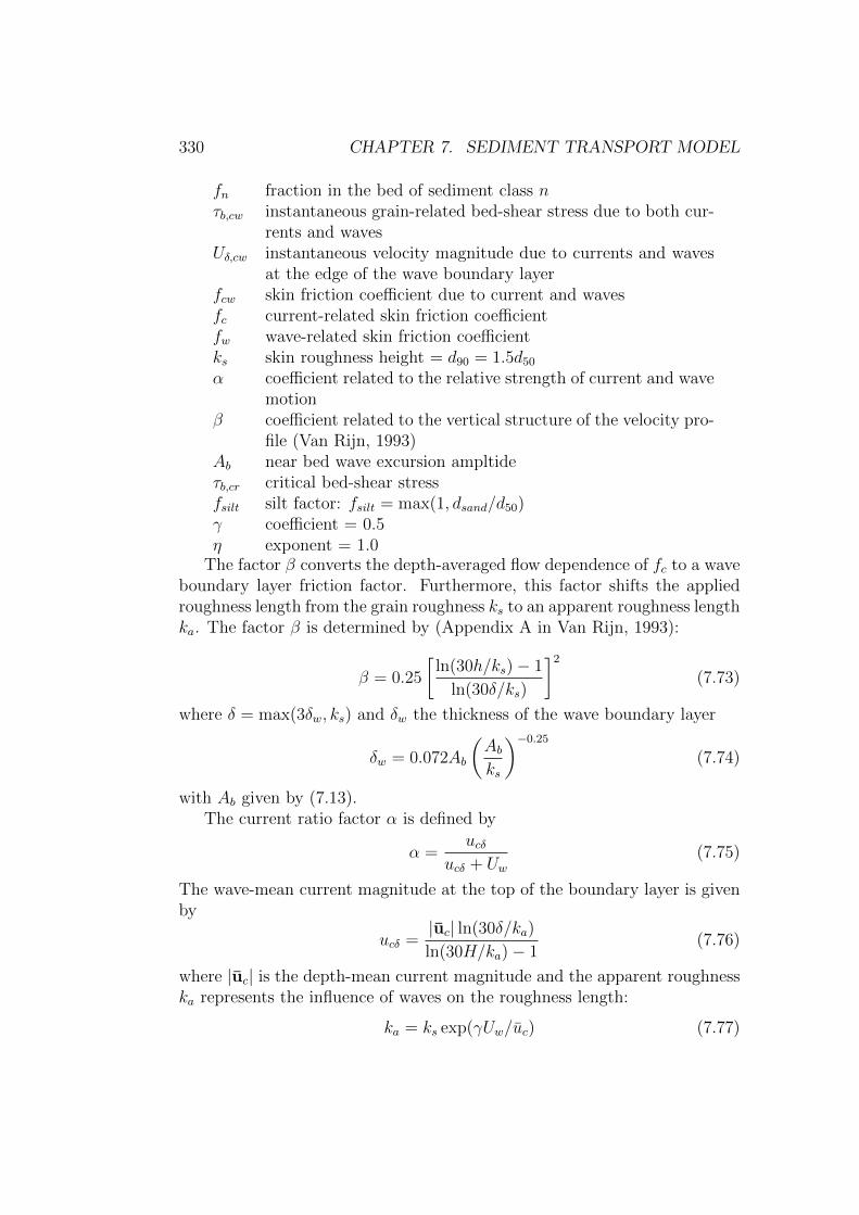
330 CHAPTER 7. SEDIMENT TRANSPORT MODEL
fn fraction in the bed of sediment class nτb,cw instantaneous grain-related bed-shear stress due to both cur-
rents and wavesUδ,cw instantaneous velocity magnitude due to currents and waves
at the edge of the wave boundary layerfcw skin friction coefficient due to current and wavesfc current-related skin friction coefficientfw wave-related skin friction coefficientks skin roughness height = d90 = 1.5d50α coefficient related to the relative strength of current and wave
motionβ coefficient related to the vertical structure of the velocity pro-
file (Van Rijn, 1993)Ab near bed wave excursion ampltideτb,cr critical bed-shear stressfsilt silt factor: fsilt = max(1, dsand/d50)γ coefficient = 0.5η exponent = 1.0
The factor β converts the depth-averaged flow dependence of fc to a waveboundary layer friction factor. Furthermore, this factor shifts the appliedroughness length from the grain roughness ks to an apparent roughness lengthka. The factor β is determined by (Appendix A in Van Rijn, 1993):
β = 0.25
[ln(30h/ks)− 1
ln(30δ/ks)
]2(7.73)
where δ = max(3δw, ks) and δw the thickness of the wave boundary layer
δw = 0.072Ab
(Abks
)−0.25(7.74)
with Ab given by (7.13).The current ratio factor α is defined by
α =ucδ
ucδ + Uw(7.75)
The wave-mean current magnitude at the top of the boundary layer is givenby
ucδ =|uc| ln(30δ/ka)
ln(30H/ka)− 1(7.76)
where |uc| is the depth-mean current magnitude and the apparent roughnesska represents the influence of waves on the roughness length:
ka = ks exp(γUw/uc) (7.77)

7.4. BED LOAD 331
γ = 0.8 + φ− 0.3φ2 (7.78)
where φ is the angle between wave propagation and current direction and Uwthe near-bed wave orbital velocity given by (7.8).
The instanteneous near-bed flow velocity magnitude due to combinedwaves and currents is determined as the magnitude of the vector sum of thecurrent and wave components
Uδ,cw(t) =[(Uw sinϕ
)2+ u2cδ + 2ucδUw cosφ sinϕ
]1/2(7.79)
where ϕ = ωwt is the wave phase.The instantaneous bed load transport vector is decomposed in a com-
ponent along the current direction and a component at right angle to thecurrent. The mean components are obtained after integration over the waveperiod, by means of the Gaussian quadrature technique (Section 7.7.3).
qbc =1
2π
∫ 2π
0
qb(t)uc,δ + Uw sinϕ cosφ
Uδ,cw(t)dϕ
qbn =1
2π
∫ 2π
0
qb(t)Uw sinϕ sinφ
Uδ,cw(t)dϕ (7.80)
Note that the transport components are calculated at U- and V-nodesseparately.
7.4.8 Van Rijn (2003)
In the current version the bed load transport equations are identical to theVan Rijn (2007a) method when this formula is selected. The difference be-tween both methods is situated in the suspended load equations (see Sec-tions 7.5.5 and 7.5.6).
7.4.9 Bed slope effects and coordinate transforms
The gradient of the bed level can have three effects:
• influence of local flow velocity
• a different critical condition for incipient motion
• a change in the bed load transport rate and direction beyond incipientmotion.

332 CHAPTER 7. SEDIMENT TRANSPORT MODEL
In COHERENS, the second and third effect can be modeled using theswitch iopt sed slope. The second effect was discussed in Section 7.3.2. Forthe third effect, a correction for the transport rate vector magnitude has tobe combined with a correction on the transport direction, i.e. the correctionhas a longitudinal component parallel to the current vector and transversecomponent, normal to the current.
The longitudinal ∂h/∂c and transverse ∂h/∂n bed slopes are given by
∂h
∂c=
1
h1
∂h
∂ξ1cosφc +
1
h2
∂h
∂ξ2sinφc (7.81)
∂h
∂n=
1
h2
∂h
∂ξ2cosφc −
1
h1
∂h
∂ξ1sinφc (7.82)
where φc is the angle between the ξ1- and current directions.The slope effects are modeled using the relation of Koch & Flokstra
(1981). They developed the following relation for a correction factor αs onthe bed load transport rate
αs = 1− βs∂h
∂c(7.83)
with βs = 1.3. They included also the effect of the slope transverse to theflow by the change in direction of δs degrees:
tan δs = βs∂h
∂n(7.84)
Note that these corrections are only applied for bed load equations and notfor total load.
The bed load formulae in the previous subsections were derived along thecurrent direction and an additional transverse component in the presence ofwaves. The components along the coordinate directions are calculated bythe following transformations
qb1 = αs
(qbc cos(φc + δs)− qbn sin(φc + δs)
)qb2 = αs
(qbc sin(φc + δs) + qbn cos(φc + δs)
)(7.85)
where
• αs = 1, βs = 0, δs = 0 in the absence of bed slope effects
• qbn = 0 in the absence of waves.

7.5. TOTAL LOAD 333
Implementation
The bed load formulae in this section are selected with the following switches
iopt sed bedeq Type of bedload equation.
1 : Meyer-Peter & Muller (1948)
2 : Engelund & Fredsøe (1976)
3 : Van Rijn (1984b)
4 : Wu et al. (2000)
5 : Soulsby (1997). This equation includes wave effects.
6 : Van Rijn (2003). This formula includes wave effects.
7 : Van Rijn (2007a). This method includes wave effects.
iopt sed slope Disables (0) or enables (1) bed slope efects using the Koch &Flokstra (1981) formulation.
7.5 Total Load
7.5.1 Engelund and Hansen (1967)
The classic formula of Engelund & Hansen (1967) has been modified byChollet & Cunge (1979) to take into account of different transport regimesand to introduce a threshold for beginnning of sediment particle motion:
qt = 0.05fn
[(s− 1)d350
g
]1/2K2H1/3θ5/2∗ (7.86)
in which fn is the fraction in the bed of sediment class n, K is the Stricklercoefficient, i.e. the inverse of the Manning coefficient, defined in (7.4) and sthe relative density of the sediment.
The need for the Strickler coefficient can be avoided by setting K2H1/3
equal to g/CD, which can be computed using (7.2) with z0 chosen equalto either the (form) roughness length from the hydrodynamic model or theskin roughness length defined in the sediment transport model. To switchbetween the two options, set iopt sed tau to the appropriate value.
In the original formulation by Engelund & Hansen (1967) θ∗ is set to θ.In the modified version of Chollet & Cunge (1979), θ∗ is defined depending

334 CHAPTER 7. SEDIMENT TRANSPORT MODEL
on the transport regime:
θ∗ = 0 if θ < 0.06 (no transport),θ∗ = [2.5(θ − 0.06)]0.5 if 0.06 < θ < 0.384 (dune regime),θ∗ = 1.065θ0.176 if 0.348 < θ < 1.08 (transition regime),θ∗ = θ if 1.08 < θ (sheet flow regime),
(7.87)
where θ is the Shields parameter, defined by (7.27).The user can choose to use the original version as well as the modified
version by setting the switch iopt sed eha. The modified version shows devi-ations of the transport calculated for bed shear below the sheet flow regime,where the original version shows result more in line with other formulae.
7.5.2 Ackers and White (1973)
A direct determination of the total sediment transport rate is provided withthe formula from Ackers & White (1973). It gives extra attention to the sub-division of non-cohesive sediment transport for coarser and finer fractions. Itwas developed using hydraulic considerations and dimensional analysis. Thecoefficients in the model have been determined by evaluation of nearly 1000experiments in the laboratory and 250 experiments in the field. Nineteendifferent transport formulae have been studied in this work.
A parameter of mobility was defined, based on the Shields parameter:
Fgr =unw∗√
(s− 1)gd
[|u|
2.46 ln(10H/d)
](1−nw)(7.88)
The parameter of transport is then defined as
Ggr = Cw
(FgrAw− 1
)mwfor Fgr > Aw
Ggr = 0 otherwise (7.89)
The total load is then calculated as follows:
(qt1, qt2) = fnGgrd
(|u|u∗
)nw(u, v) = fnGgrdC
−nw/2D (u, v) (7.90)
with d = d35, fn the fraction of size class n in the bed and |u| the magnitudeof the depth averaged current.
This transport formula was derived by uniting bed load and suspendedload transport relations in one function through a transition in the dimen-sionless d∗ parameter. A revised set of values for the parameters mw and

7.5. TOTAL LOAD 335
Cw which are used in the current implementation, have been derived afterexperiments in 1990:
nw = 1− 0.243 ln d∗
mw = 1.67 + 6.83/d∗
lnCw = 2.79 ln d∗ − 0.426(ln d∗)2 − 7.97
Aw = 0.14 + 0.23/d1/2∗ (7.91)
with d∗ = min(60,max(1, d∗)).Since this total load formula was developed using a d35 grain size diameter,
the user should also give this sieve size instead of d50 when the informationis available.
7.5.3 Madsen and Grant (1976)
The Madsen & Grant (1976) formula is a total load formula determining theinstantaneous transport rate vector qt, for one sediment grain size class:
qt = 40fnwsdnθ3cw
Ucw(t)
|Ucw(t)|(7.92)
in which ws is the particle fall velocity, dn the grain size of class n, withfraction fn, θcw the instantaneous Shield parameter of dimensionless shearstress due to currents and waves and Ucw the current due to current andwaves, whose magnitude is given by (7.79).
The Shields parameter is computed here with the velocity due waves andcurrents and with a combined friction factor for waves and currents:
θcw(t) =fcw|Ucw(t)|2
2(s− 1)gd50(7.93)
with
fcw = αfc + (1− α)fw (7.94)
α =ucδ
ucδ + Uw(7.95)
fc = 0.32
[ln
(H
z0s
)− 1
]−2(7.96)
ucδ =u∗κ
ln(30δ
z0
)(7.97)

336 CHAPTER 7. SEDIMENT TRANSPORT MODEL
where fc is the friction factor due to currents and fw the wave-related frictionfactor given by (7.18). The wave boundary layer thickness δ is the same asthe one for the Van Rijn (2007a) bed load formula.
The mean total load is obtained by decomposing the instantaneous sedi-ment total load vector into components, along and transverse to the currentdirection, and integration over the wave period using (7.80) with qb replacedby qt. The components along the coordinate axes are obtained using (7.85)without slope effects (i.e. αs = 1, βs = 0, δs = 0).
The integration over the wave period is executed in the code with thenumerical integration method of Gaussian quadrature. For details about theapplied method see Section 7.7.3. The number of data points needed in thismethod to reach a stable solution is optimised for the Madsen & Grant (1976)method. The fact that the transport is determined with the fifth power of theShields number makes that the oscillating signal of the wave-current velocityresults in a very peaked instantaneous transport. The consequence is that arelatively high number of points is needed to capture the sharp peak in thetransport during maximal near-bed velocity. The optimal number for thismethod was determined at 15 points per wave period, see Figure 7.1.
The procedure is repeated for each class of sediment grain size defined bythe user.
7.5.4 Wu et al (2000)
The calculation procedure for bed load transport is described in Section 7.4.5.Adding the following equation for suspended load to the bed load formularesults in the total sediment transport due currents only:
qs,n = 0.262.10−4√
(s− 1)gd3[(
τbτcr,n
− 1
)|u|ws,n
]1.74(7.98)
Here, the settling velocity is calculated with equation (7.42) of Zhang &Xie (1993) and the critical shear stress using relation (7.33) from Wu et al.(2000).
7.5.5 Van Rijn (2003)
In an unpublished paper Van Rijn (2003) describes approximate formulaefor the bed and suspended load under combined currents and waves. A va-lidity range is given for d50 between 0.1 and 0.5 mm sand, water depthsbetween 0.25 and 20 m, current velocities between 0 and 2 m/s and relativewave heights Hs/H between 0 and 0.5. In this code, the bed load is not

7.5. TOTAL LOAD 337
Fig
ure
7.1:
Con
verg
ence
ofG
auss
-Leg
endre
quad
ratu
refo
rw
ave
per
iod
inte
grat
ion
ofin
stan
taneo
us
sedim
ent
tran
s-p
ort.
Diff
eren
tp
eak
orbit
alve
loci
ties
and
wav
e-cu
rren
tan
gles
are
consi
der
ed.

338 CHAPTER 7. SEDIMENT TRANSPORT MODEL
computed following the approximate formula, but with the fully integratedinstantaneous oscillating transport, as described in Section 7.4.7. The sus-pended load, however, is computed using the explicit approximation formulaof Van Rijn (2003).
The suspended sediment transport due to currents and waves is calculatedby
qs = qsc + qsw (7.99)
which is the sum of the current-related suspended transport (with wave agita-tion), directed in the main current direction and the wave-related suspendedtransport in the wave propagation direction (associated with wave asymme-try). For simplicity, it is assumed in the following that there is only one grainsize class in the sediment bed. In case of multiple fractions, the proceduresare repeated for all classes, and the transports are multiplied with each class’fraction in bed.
7.5.5.1 Current-related part
The current related part of the sediment transport is calculated as:
qsc = (Fc + Fw)|uc|Hca (7.100)
Here, Fc and Fw are correction factors representing the depth-averaged con-centration profile (relative to ca), for current and waves respectively. Theyare defined as follows
Fc = G(Zc) (7.101)
Fw = G(Zw) (7.102)
where the function G(Z) reads:
G(Z) =
[(a/H)Z − (a/H)1.2
][(1.2− Z)(1− a/H)Z ]
(7.103)
Zc =ws
βcκu∗c+ 2.5
(wsu∗c
)0.8(cacmax
)0.4
(7.104)
Zw = 4
(H
Href
)0.6(wsTPHS
)0.8
(7.105)
where βc = 1 + 2(ws/u∗)2, a the reference height (see Section 7.6.3.1), Href
the reference water depth taken as 5 m, TP the peak period of the waves,HS the significant wave height and cmax the maximal concentration, whichis taken equal to 0.65 for sand.

7.5. TOTAL LOAD 339
The appropriate expression for the reference concentration ca is the onegiven in equation (7.125), but modified for wave-current interaction. TheT -parameter (7.61) becomes then
Tn = max
(τ eb,cwτcr,n
− 1, 0
)(7.106)
where τ eb,cw = τ eb,c+τ eb,w is the time-(wave-) averaged effective bed shear stressand τcr,n the critical bed shear stress for sediment class n.
The effective current-related bed-shear τ eb,c is determined by:
τ eb,c = µcαcwτb,c (7.107)
here, µc is the current-related efficiency factor, transforming the friction fac-tor from total friction to grain-related friction, since the oscillating characterof the flow does not permit it to feel bed forms with longer wavelength thanthe near-bed wave excursion. Also related to this effect is the wave-currentinteraction factor αcw. The former and latter parameters are defined as:
µc = f ec /fc =
[log(H/30z0)
log(H/1.5d50)
]2(7.108)
αcw =
[ln(90δw/ka)
ln(90δw/ks)
]2 [ln(30H/ks)− 1
ln(30H/ka)− 1
]2(7.109)
αcw,max = 1 (7.110)
with δw the wave boundary layer thickness and ka the apparent roughness.For definitions, see Section 7.4.7. Note that the skin roughness height is setto 1.5d50 which is the actual median grain size in the bed at each locationfrom the particle size distribution in the highest bed layer.
The effective wave-related bed-shear τ eb,w is in turn determined by:
τ eb,w = µwτb,w (7.111)
In the 2003 version of the van Rijn model, µw is given by 0.125(1.5−Hs/H)2.This parameter will be different in the 2007 version described in the next sec-tion. The bed shear stresses due to waves and due to currents are determinedusing the same friction factors as in the bed load transport model, see Sec-tion 7.4.7.
7.5.5.2 Wave-related part
This part of the suspended load – with equal values in the 2003 and 2007versions of the van Rijn model – is dependent on the wave asymmetry in

340 CHAPTER 7. SEDIMENT TRANSPORT MODEL
terms of onshore and offshore directed peak velocities. These velocities havebeen computed using the method of Grasmeijer & Van Rijn (1998). Thewave propagation directed suspended transport is given by:
qsw,n = γfnUALT (7.112)
with
qsw,n volumetric suspended sediment transport of classn [m2/s]
UA =(U4δ,f−U
4δ,b) /(U3
on+U3off )
velocity asymmetry [m/s]
LT = 0.007dnMe suspended sediment load [m]
Me =(ve−vc)2 /((s−1)gdn) Sediment mobility number due to waves and cur-rents
Uδ,f Near-bed orbital velocity peak in onshore (for-ward) direction [m/s]
Uδ,b Near-bed orbital velocity peak in offshore (back-ward) direction [m/s]
ve =√U2 + U2
δ,f effective velocity due to currents and waves [m/s]
vc = 0.19d0.1n ln(2h/dn) critical velocity for 0.1 mm < dn < 0.5 mm [m/s]vc = 8.50d0.6n ln(2h/dn) critical velocity for dn > 0.5 mm [m/s]dn grain size of sediment class n [m]γ phase lag coefficient = 0.2
A number of assumptions have been made during the development of thissimplified approximative formulation: a bed roughness length ks of 0.03m,wave-current angle of 90 degrees, temperature of 150C; salinity of 30 ppt. Theonshore and offshore peaks of the asymmetric wave boundary velocities Uδ,fand Uδ,b are computed using the method of Grasmeijer & Van Rijn (1998),which will not be reproduced here.
Effectively, in this method, the critical condition for initiation of motionis defined specifically. The methods used in other parts of the code fordetermination of critical shear are not applied for the wave part of suspendedload.
7.5.6 Van Rijn (2007a)
The Van Rijn (2007a) method is very similar to the 2003 version, with adifferent formulation for some of the parameters: the turbulence dampingfactor and the wave-related efficiency factor.
7.5. TOTAL LOAD 341
Due to the relation adopted for turbulence damping due to high sedimentconcentrations, the modified Rouse number in the approximative formulationfor current-related suspended load (Zc in equation (7.104)) takes a differentform
Zc =ws
βcκu∗φd(7.113)
Here, φd is the turbulence damping function used, originally varying withconcentration, but here evaluated for the reference concentration
φd = 1 + (ca/cmax)0.8 − 2(ca/cmax)
0.4 (7.114)
The wave-related efficiency factor µw takes a different form in this formu-lation. It is made dependent of the dimensionless particle diameter ratherthan the wave height relative to the water depth:
µw =
0.35 if d∗ < 20.7/d∗ if 2 < d∗ < 50.14 if 5 < d∗
(7.115)
Implementation
The type of total load formulation is selected with the following switches
iopt sed toteq Method for total load transport
1: Engelund & Hansen (1967). The precise form is also determined bythe switch iopt sed eha.
2: Ackers & White (1973)
3: Madsen & Grant (1976). This equation includes wave effects.
4: Wu et al. (2000). Total load is calculated as the sum of suspendedand bed load.
5: Van Rijn (2003). This equation includes wave effects and total loadis the sum of suspended and bed load.
6: Van Rijn (2007a). This equation includes wave effects and total loadis the sum of suspended and bed load.
iopt sed eha Switch to select the type of formulation in the Engelund-Hansentotal load equation (7.86)
1: original form
2: Chollet & Cunge (1979) form as function of θ∗

342 CHAPTER 7. SEDIMENT TRANSPORT MODEL
7.6 Suspended sediment transport
7.6.1 Three-dimensional sediment transport
In COHERENS multiple sediment fractions can be taken, each with its owndiameter, settling velocity, critical shear stres, . . . . In an orthogonal curvilin-ear coordinate system, the sediment concentration of each sediment fractionis governed by the following advection-diffusion equation for the volumetricsediment concentration fraction c (with the subscript n omitted):
1
h3
∂
∂t(h3c) +
1
h1h2h3
(∂
∂ξ1(h2h3(u− us)c) +
∂
∂ξ2(h1h3(v − vs)c)
)+
1
h3
∂
∂s
(h3(ω − ws)c
)=
1
h3
∂
∂s
(DV
h3
∂c
∂s
)+
1
h1h2h3
( ∂
∂ξ1
DHh2h3h1
∂c
∂ξ1+
∂
∂ξ2
DHh1h3h1
∂c
∂ξ2
)+
Qsed
h1h2h3(7.116)
where DV = λsT , DH = λH are the vertical, respectively horizontal diffusioncoefficients for sediments, ws the settling velocity, defined in Section 7.3.3 andQsed a user defined source term. More information on the used coordinatesystems can be found in Section 4.1. In the 3-D version of the transportequation, erosion and depositions of sediment enter through the boundaryconditions (Section 7.6.3).
Equation (7.116) is the same as the scalar transport equation (4.76) fora scalar quantity ψ except that the equation now contains an extra verticaladvective term for the settling velocity. Since the settling velocity is directedalong the vertical which does not coincide with the transformed vertical di-rection normal to the iso-σ surfaces, the horizontal advective currents needto be adjusted by adding a correction for settling
us = −wsh1
∂z
∂ξ1
∣∣∣s= −ws
h3h1
∂s
∂ξ1
∣∣∣z
(7.117)
vs = −wsh2
∂z
∂ξ2
∣∣∣s= −ws
h3h2
∂s
∂ξ2
∣∣∣z
(7.118)
7.6.2 Two-dimensional sediment transport
As explained in Section 4.3.2, the advection-diffusion equations for sedimentscan also be solved in depth-averaged form. In that case, erosion E anddeposition D, used to determine the bottom boundary condition in the 3-D

7.6. SUSPENDED SEDIMENT TRANSPORT 343
case (see below), are modeled by source terms in the depth averaged sedimentconcentration equation
∂c
∂t+
1
h1h2
(∂
∂ξ1h2cu+
∂
∂ξ2h1cv
)=
1
h1h2
(∂
∂ξ1DH
h2h1
∂c
∂ξ1+
∂
∂ξ2DH
h1h2
∂c
∂ξ2
)+E −DH
(7.119)
For details see Section 4.3.2.
7.6.3 Erosion and deposition
Erosion and deposition have a double influence. On the one hand, the erosionand deposition provide the bottom boundary conditions for the advection-diffusion equation of sediment transport. On the other hand, they providean important source term in the equation for the bed-level elevation for themorphology. In this section, the modeling of the erosion and deposition termsis described. This is first done for three-dimensional situations, where theerosion and deposition terms are introduced through the near-bed boundaryconditions. These terms are described separately for sand and mud, becausethey are calculated in a different way. This is followed by a description oferosion and deposition in two-dimensional situations, where they are repre-sented as a source term.
7.6.3.1 Erosion and deposition of sand in 3-D
The following equation is used as the boundary condition near the bed forthe suspended sediment transport equation (taken at a reference height aabove the bed)
−DV (a)∂cn∂z
(a)− ws,in(a)cn(a) = En −Dn (7.120)
Here, En is the erosion of sediment fraction n, Dn the deposition, cn thevolumetric sediment concentration, and ws,n the settling velocity of fractionn. Note that because the volume concentrations are used in COHERENS, thedimensions of the erosion and deposition are m/s.
The deposition flux is given as
Dn = ws,n(a)cn(a) (7.121)
Using this expression, the bottom boundary conditions reduces to thefollowing Neumann boundary condition:
−DV (a)∂cn∂z
∣∣∣a
= En (7.122)

344 CHAPTER 7. SEDIMENT TRANSPORT MODEL
Garcia & Parker (1991) showed that the flux can be expressed as an non-dimensional flux E∗ ≡ E/ws and that in situations not too far from equili-brium, this non-dimensional entrainment is equal to the near bed referenceconcentration (i.e. E∗ = ca). Therefore one can write:
−DV (a)∂cn∂z
∣∣∣a
= fnws,n(a)ca,n (7.123)
Here ca,n is the near-bed reference (equilibrium) sediment concentration ata reference height an for sediment size class n with fractional amount fn atthe bed.
In COHERENS, the near bed reference concentration for sand is calculatedeither by the method of Smith & McLean (1977) or by the one in Van Rijn(1984a), which can be selected with the switch iopt sed bbc.
The near-bed boundary condition of Smith & McLean (1977) is given foreach fraction n by:
ca,n = 0.0024cmaxTn
1 + 0.0024Tna = ks + 26.3(θn − θcr,n)dn
ks = 30z0 (7.124)
Here, cmax is the maximum possible concentration, i.e. the concentration ofa bed packed with sediment, Tn the normalised excess shear stress definedby (7.61), θ the Shield parameter (7.27), ks the skin roughness height and z0the skin roughness length.
The near bed boundary condition of Van Rijn (1984a) is given by:
ca,n = 0.015dnT
1.5n
and0.3∗n(7.125)
with d∗ defined by (7.29). The reference level a (either half the size of thedunes or the roughness length scale ks) is limited to be between 0.01H and0.1H.
It may occur that the reference level an is not located within the bottomgrid cell where the bottom boundary condition is applied. The methods usedin COHERENS to overcome this problem are described in Section 7.7.1. Theinfluence of waves on the erosion of sediment is included in this equation onlyby the change in the bed shear stress due to the near bed wave motion usingthe equation of Soulsby (1997).

7.6. SUSPENDED SEDIMENT TRANSPORT 345
7.6.3.2 Erosion of cohesive sediment in 3-D
Erosion of cohesive sediments is calculated with the equation based on thedata of Partheniades (1965)
En = fnM
(τb − τcr,nτcr,n
)npfor τb > τcr,n (7.126)
Here En is the erosion rate, M is an erosion rate parameter (m/s), τbthe bed shear stress, τcr the critical shear stress threshold for erosion and npan empirical parameter (normally equal to unity). The parameters M andτcr,n need to be determined, which can be difficult in practice, because theydepend on the material, its consolidation as well as biological and chemicalcharacteristics of the bed, thus they can vary in space and time and fn is theamount of this fraction in the bed. In COHERENS, the critical shear stress isdetermined using one of the methods, described in Section 7.3.2. Note thatthe unit of M (m/s) and τcr,n (m2/s2) in the code is different from usual,where the units of these quantities are respectively kg/m2/s and N/m2.
The implementation of the three-dimensional erosion of cohesive sedimentdiffers from sand in that no reference concentration is calculated, and noreference height has to be specified. Just as for sand, wave effects are onlyincluded through the changes in the bed shear stress.
7.6.3.3 Erosion-deposition of sand in 2-D
In two dimensional calculations, the erosion and deposition of sand are cal-culated from the difference between the depth averaged concentrations andthe depth averaged equilibrium concentration. A time scale Te,n is used inwhich the sediment concentration adapts to the equilibrium concentration.This represents the fact that deposition depends on the near-bed sedimentconcentration, rather than the depth averaged value and thus that the se-diment concentration profile needs some time to adapt to the equilibriumprofile (e.g. Galappatti & Vreugdenhil, 1985). The equations that are usedfor the erosion deposition term are
En −Dn =H
Te,n(ce,n − cn) (7.127)
The equilibrium concentration ce can be calculated in different ways,which are selected by the switch iopt sed ceqeq. The default option is tocalculate the equilibrium concentration by taking the depth average of theRouse profile numerically (see Section 7.7.3 for the numerical method), which

346 CHAPTER 7. SEDIMENT TRANSPORT MODEL
is given byceqca
=
[H − zz
a
H − a
]R(7.128)
where a is the reference level, H the total water depth, z = z + h theheight above the sea bed, ca the reference concentration, R = ws/βκu∗ theRouse number, ws the particle fall velocity, u∗ the skin shear velocity, β theinverse of the Prandtl-Schmidt number (see Section 7.6.4) and κ the vonKarman constant. The exponent expresses the relative importance of thesuspended load, where it is equal to about 5 for bed load only and decreasesto unity for suspended load up to the surface (Van Rijn, 1993). The referenceconcentration is defined in Section 7.6.3.1.
Another way to calculate the depth averaged sediment concentrations isby using one of the fomulae for suspended transport, described in Section 7.5.The depth averaged equilibrium concentration is then given by
ce =qs,e|U|
(7.129)
Here qs,e is the equilibrium suspended sediment transport and |U| themagnitude of the depth-integrated current (in m2/s).
The adaptation time scale Te is given by:
Te =H
wsT∗ (7.130)
Here, T∗ is a non-dimensional correction factor, which depends on the shapeof the sediment concentration profile, parametrized by the Rouse number Rdefined below. For COHERENS, this relation was obtained by performingsimulations with COHERENS in water column (1DV) mode and determiningthe adaptation time scale from the data (see Figure 7.2). Through this dataan eight order polynomial was fitted:
T∗ = p1R8 + p2R
7 + p3R6 + p4R
5 + p5R4 + p6R
3 + p7R2 + p8R+ p9 (7.131)
with:R = min(wsb/u∗, 1.14) (7.132)
and
p1 = 67.342 p2 = −321.0 p3 = 614.14
p4 = −592.75 p5 = 292.15 p6 = −62.141
p7 = 3.667 p8 = −2.2571 p9 = 0.97978 (7.133)
and wsb the settling velocity at the bottom.

7.6. SUSPENDED SEDIMENT TRANSPORT 347
0 0.2 0.4 0.6 0.8 10
0.1
0.2
0.3
0.4
0.5
0.6
0.7
0.8
0.9
1
ws/u
*
T w
s/h
Data 1DV simulation 8th degree polynomial
Figure 7.2: Numerically determined time scale and fitted polynomial
7.6.3.4 Erosion-deposition of cohesive sediment in 2-D
For cohesive sediments, the erosion and deposition rates in 2-D are obtainedin similar way as for sand, using an equilibrium time schale and a depthaveraged concentration (Section 7.6.3.3). For cohesive sediment, the only wayin which the depth averaged equilibrium concentration can be calculated is byaveraging the Rouse profile (equation 7.128). However, a near-bed referenceconcentration and reference location are needed to obtain the depth averagedconcentrations. The near bed reference concentration is obtained from thenear bed erosion rate E using
ca =E
ws(a)(7.134)
The near bed reference location a is, in the 2-D case, an extra tunableparameter height c cst. This is not very different from the usual approachto use a threshold of deposition as an extra tunable parameter for simu-lating cohesive sediment transport. However, the present approach has theadvantage that unphysical results that may result from the threshold of de-position method (such as the unlimited erosion leading to unphysically highsediment concentrations) are avoided. The same time schale is used as forthe calculation of depth averaged sand transport.

348 CHAPTER 7. SEDIMENT TRANSPORT MODEL
7.6.4 Sediment diffusivity
7.6.4.1 Without wave effects
It has been found experimentally that the diffusivity of sediment is not alwaysequal to the eddy diffusivity. For practical purposes, the sediment diffusivityDV is assumed to be proportional to the eddy viscosity
DV = βνT (7.135)
Here, β is the inverse of the Prandtl-Schmidt number σT and νT the eddyviscosity defined in Section 4.4. Different relations have been proposed forthe β factor. In COHERENS, β can be either a constant or calculated withthe equation of Van Rijn (1984b). Based on the work of (Coleman, 1970),he found that it can be taken as a function of the settling velocity
β = 1 + 2
(wsu∗
)2
(7.136)
For practical applications, β is limited to values between 1 and 1.5.
7.6.4.2 With waves effects
The vertical sediment diffusivity due to combined waves and currents DV,cw
is calculated from the sediment diffusivity due to current and waves using(Van Rijn, 2007b)
DV,cw =√
(DV,c)2 + (DV,w)2 (7.137)
Here, DV,c = βνT is the sediment diffusivity in the absence of waves and DV,w
an additional component due to waves.The wave related sediment diffusivity DV,w is calculated by separate ex-
pressions for the upper half of the water column and for the near-bed mixinglayer. Between the two layers, a linear interpolation is performed (Van Rijn,2007b)
DV,w = DV,w,max = 0.035γbrHHs/Tp ≤ 0.05 m2/s for 0.5H ≤ z
DV,w = DV,w,bed + (DV,w,max −DV,w,bed)[
z−δs0.5H−δs
]for δs < z < 0.5H
DV,w = DV,w,bed = 0.018γbrβwδsUδ,r for z ≤ δs(7.138)
where z is the distance above the sea bed, Uδ,r the near-bed peak orbitalvelocity Uw, given by (7.8), Tp the peak wave frequency and δs the thicknessof the mixing layer
δs = 0.072γbrAδ(Aδ/kw)−0.25 (7.139)

7.6. SUSPENDED SEDIMENT TRANSPORT 349
Here, Aδ is the near-bottom orbital excursion Ab, given by (7.13), kw thewave-related bed roughness height,
γbr = 1 + (Hs/H − 0.4)0.4 (7.140)
a coefficient related to wave breaking (= 1 for Hs/H ≤ 0.4), and
βw = 1 + 2(ws/u∗,w)2 (7.141)
where u∗w is the wave-related bed-shear velocity.
7.6.5 Boundary conditions
Bottom boundary conditions for sediment are defined through erosion anddeposition and discussed in Section 7.6.3.
At the free surface, a vertical zero-flux condition is used for the suspendedsediment:
DV∂cn∂z
+ ws,ncn = 0 (7.142)
The lateral boundary conditions are the same as the ones in discussed inSection 4.10.2.2.
Implementation
The following switches are used for the transport of suspended sediment:
iopt sed mode Type of mode for applying the sediment transport model
1: bedload transport only computed by a formula, which is determinedby iopt sed bedeq
2: suspended load transport only (computed with the advection-diffusionequation)
3: bedload and suspended transport (i.e. option 1 and 2 together)
4: total load transport computed with a formula, which is determinedby iopt sed toteq
iopt sed nodim The number of dimensions used in the sediment formula-tion.
2: depth averaged transport3
3: 3-D sediment transport.
3Note that iopt sed nodim is always set to 2 if iopt grid nodim = 2.

350 CHAPTER 7. SEDIMENT TRANSPORT MODEL
iopt sed type The type of sediment that is used
1: sand (non-cohesive)
2: mud (cohesive)
iopt sed bbc The type of equation for bed boundary condition at the seabed
0: no bed boundary conditions (no flux to and from the bed)
1: Smith & McLean (1977)
2: Van Rijn (1984a)
3: Partheniades (1965)
iopt sed ceqeq The type of model for determining the equilibrium sedimentconcentration
1: numerical integration of the Rouse profile
2: Using qt/U determined with the equation of Engelund & Hansen(1967). The precise form is also determined by the switch iopt sed eha.
3: using qt/U determined with the equation of Ackers & White (1973).
4: Using qs/U determined with the equation of Van Rijn (2003). Thisformulation is very similar to Van Rijn (1984b), but takes wavestresses into account.
5: using qs/U determined with the equation of Wu et al. (2000)
iopt sed beta The type of equation used for β, the ratio between the eddyviscosity and eddy diffusivity
1: β = 1.
2: user defined value of β (beta cst).
3: Van Rijn (1984b).
iopt sed wave diff Selects the turbulent diffusion coefficient due to waves.
0: No diffusion coefficient
1: According to Van Rijn (2007b)
7.7 Numerical methods
This section describes the numerical methods that are specifically used inthe sediment transport module. The methods are generally the same as the

7.7. NUMERICAL METHODS 351
ones for a scalar quantity, as described in Section 5.5. However, there aresome differences, mainly related to the modeling of erosion and deposition,which are discussed here.
7.7.1 Erosion-deposition
7.7.1.1 Three-dimensional sediment transport
In three-dimensional simulations, erosion and deposition come into play throughthe near-bed boundary condition. For mud, the erosion rate is given directlyby the equation of Partheniades (1965). For sand, the erosion E is calcu-lated from the near bed reference concentration ca at a height a above thebed using E = wsca. However, the height a does not normally coincide withthe used computational grid. Hence, a transformation has to be made, suchthat the erosion is calculated at a location coinciding with the computationalgrid.
In COHERENS, three methods are available to do this, which can be setwith the switch iopt sed bbc type. The first two options are based on themethod used in the EFDC model. In this method, the flux is calculatedbased on an averaged of either the lowest cell (iopt sed bbc type = 1) or thecell in which a lies (iopt sed bbc type =2). At a given reference level a, thenet upward flux is given by
F (a) = ws(ca − c) (7.143)
Integrating this expression over the bottom cell gives the bottom flux intothat bottom cell, F0:
F0 = ws(ceq − c1) (7.144)
were ceq is the averaged equilibrium concentration for the bottom cell, c1 isthe sediment concentration in the bottom cell. The determination of ceq canbe done by solving equation (7.146) below for F0, and averaging over thebottom cell by integration between z0 and z1, i.e. the W-nodes below andabove the bottom cell. In case the reference level a is located above the near-bed cell and iopt sed bbc type =2, the nth cell is integrated (the ‘referencelayer’), from zn−1 up to zn, and the c1 term in equation (7.144) becomes cn,yielding:
F0 = ws
(ca
∆zn
∫ zn
zn−1
(az
)Rdz − 1
∆zn
∫ zn
zn−1
cdz
)(7.145)
where ∆zn is the thickness of the nth cell, with the reference level a locatedin the nth cell.

352 CHAPTER 7. SEDIMENT TRANSPORT MODEL
Herein, the following expression is used for the non-equilibrium near bedsediment profile (derived assuming a linear varying eddy viscosity near thebed)
c = ca
(az
)R− F0
ws(7.146)
Combining this expression with equation (7.144) gives
ceq =ca
∆zn
∫ zn
zn−1
(az
)Rdz (7.147)
For R 6= 1, this gives
ceq =aRca
∆zn(1−R)
[z1−Rn − z1−Rn−1
](7.148)
and for R = 1
ceq =aca∆zn
[ln zn − ln zn−1] (7.149)
The range of values for the Rouse number R are limited by the theo-retical maximum of 2.5, since no suspension can exist when the settlingvelocity is larger than the shear velocity. When the method of cell-averagedreference concentration described above is used while the reference level islocated within the bottom cell, the integrated profile (equations (7.148)-(7.149)) starts from the bottom of the near-bed cell, at level z0. Since theRouse profile is not valid that close to the bed, another lower limit for inte-gration is used, with the minimum set at the Nikuradze roughness ks = 30z0.The level z0, in turn, is the level at which the assumed logarithmic velocityprofile becomes equal to zero.
This method with iopt sed bbc type =2 can give very accurate results,provided that a high resolution is used near the bed. However, when theresolution is relatively low (and thus the cells near the bed are relativelylarge), the averaging of the profile leads to an overestimation of the concen-trations in the lowest cells and therefore in sediment concentrations that aretoo high. Therefore, this method is not recommended for practical applica-tions. Instead, another method should be used by setting iopt sed bbc type= 3. In this method, the Rouse profile (equation (7.128)) is used to calculatethe sediment concentration from the given boundary condition at the firstC-node above the bed.
The deposition flux is just an advection term from the lowest cell. Thetype discretisation of this term at the bed is determined by the switchiopt scal depos. The options are

7.7. NUMERICAL METHODS 353
• No deposition flux (all sediment remains inside the computation do-main). This is useful for simulating some laboratory experiments.
• First order discretisation
• Second order discretisation
The first order discretisation of the deposition flux D is an upwind dis-cretisation that is given by:
D = ww1 cc1 (7.150)
The second order discretisation of the deposition flux uses linear extrap-olation to obtain an estimation of the sediment concentration at the lowestW-node. It is given by
Dij = ws;ij1
[(1 +
hc3;ij12hw3;ij2
)cij1 −
hc3;ij12hw3;ij2
cij2
](7.151)
7.7.1.2 Time integration of sediment transport
In 2-D mode, the source/sink term is integrated semi-implicitly in time
E −D =Hn+1
Te
(ce − θvcn+1 − (1− θv)cn
)(7.152)
In case of 3-D simulations, erosion is taken explicitly whereas deposition isintegrated semi-implicitly with the implicity factor θa which is the same asthe one used for the vertical advective term in scalar transport equations (seeSection 5.5.3).
7.7.2 Bed slope factors
Using the notations of Section 7.4.9, one has
cos(φc + δs) = cosφc cos δs − sinφc sin δs
sin(φc + δs) = sinφc cos δs + cosφc sin δs (7.153)
Letting
β∗ = βs∂h
∂n= tan δs (7.154)
one has
cos δs = cos arctan β∗ =1√
1 + β2∗

354 CHAPTER 7. SEDIMENT TRANSPORT MODEL
sin δs = sin arctan β∗ =β∗√
1 + β2∗
(7.155)
so that
cos(φc + δs) =cosφc − β∗ sinφc√
1 + β2∗
sin(φc + δs) =sinφc + β∗ cosφc√
1 + β2∗
(7.156)
7.7.3 Gaussian-Legendre quadrature
In COHERENS, numerical integration needs to be performed in two cases:
• to calculate phase averages from instantaneous values in the load for-mulae of Madsen & Grant (1976) and Van Rijn (2003, 2007b)
• to determine the equilibrium concentration by taking the vertical av-erage of the Rouse profile (7.128).
The integrals are calculated by applying Gaussian quadrature. The integralof a function f(x) between a and b is calculated as:∫ b
a
f(x)dx ' b− a2
n∑i=1
wif
(b− a
2xi +
a+ b
2
)(7.157)
Here, n is the number of points in the integration xi are the locations ofthe nodes where the function is evaluated and wi are the weighting factors.The locations xi are the roots of the n-th order Legendre polynomial Pn andwi is determined by
wi =2
(1− xi)2
(dPn(xi)
dx
)−2(7.158)
The locations and weight factors are obtained by calling the routinegauss quad with, usually, a user-applied value n.
The phase average of a function f(ϕ) with ϕ = ωt, is then given by
F =1
2π
∫ 2π
0
f(ϕ) dϕ ' 1
2
n∑i=1
wif(ϕi) (7.159)
with ϕi = π(1 + xi).

7.7. NUMERICAL METHODS 355
The equilibrium concentration ce is given by
ce 'caH
∫ H
a
[H − zz
a
H − a]R
dz (7.160)
Letting φ = ln(z/H), a∗ = a/H and applying (7.157) one obtains
ce = ca( a∗
1− a∗)R ∫ 0
ln a∗
eφ(e−φ − 1
)Rdφ
' −ca2
( a∗1− a∗
)Rln a∗
n∑i=1
wieφi(e−φi − 1
)R(7.161)
with φi = 12(1− xi) ln a∗.
7.7.4 Bartnicki filter
Negative concentrations may arise by application of the bottom boundaryconditions. In order to prevent negative sediment concentrations, a Bart-nicki (1989) filter can be used with the switch iopt sed filter. This filter elim-inates negative sediment concentrations, while conserving the total sedimentvolume. It is based on the assumption that the amount of negative con-centration is much smaller than the amount of positive concentrations. TheBartnicki filter performs, at each time step, the following steps iterativelyuntil no negative concentrations exist in the model.
• The total volume of negative concentrations is determined: M− =∑ijk cijk(cijk < 0)∆Vijk where ∆Vijk = h1;ijh2;ijh3;ijk is the volume
of a grid cell.
• The total volume of the cells with a positive concentration (larger than0) is determined: V+ =
∑ijk(cijk > 0)∆Vijk.
• The average difference volume is determined: M+ = M−/V+.
• The concentration in cells with a negative concentration is set to zero.
• M+ is added to the concentration in cells with a positive concentration.
Implementation
Numerical methods, described in this section, are selected with the followingswitches:

356 CHAPTER 7. SEDIMENT TRANSPORT MODEL
iopt sed bbc type Selects the method to transpose the near bed boundarycondition to the computational grid. It is strongly recommended not tochange the default value of 3.
1: EFDC method applied to lowest cell (not recommended)
2: EFDC method applied to the first the cell above (not recommended)
3: Using the Rouse profile
iopt sed filter Disables (0) or enables (1) the application of the Bartnicki filterto prevent the occurrence of negative concentrations .