Chapter 7 Turbidity Modeling with DSM2 - Californiabaydeltaoffice.water.ca.gov/modeling/deltamodeling/AR2011/Method... · Chapter 7 Turbidity Modeling with DSM2 ... 7-12 Figure 7-12

Methodology for Flow and Salinity Estimates in the Sacramento-San Joaquin Delta and Suisun Marsh

32nd Annual Progress Report June 2011

Chapter 7 Turbidity Modeling with DSM2 Authors: Lianwu Liu and Prabhjot Sandhu,

Delta Modeling Section, Bay-Delta Office, California Department of Water Resources

Methodology for Flow and Salinity Estimates 32nd Annual Progress Report

Page 7-ii Turbidity Modeling with DSM2


Page 7-iii Turbidity Modeling with DSM2

Contents

7 Turbidity Modeling with DSM2 .............................................................................................. 7-1

7.1 Introduction .................................................................................................................. 7-1

7.2 Turbidity Modeling with DSM2 ..................................................................................... 7-1

7.3 Boundary Conditions..................................................................................................... 7-2

7.4 2010 Wet Season Calibration ........................................................................................ 7-2

7.5 Discussion of Model limitations .................................................................................... 7-3

7.6 Summary ....................................................................................................................... 7-5

7.7 Acknowledgments ......................................................................................................... 7-5

7.8 References .................................................................................................................... 7-5

Figures

Figure 7-1 CDEC turbidity stations ........................................................................................................................... 7-6

Figure 7-2 Calibrated settling rate values ............................................................................................................... 7-7

Figure 7-3 Turbidity comparison, Sacramento River at Rio Vista (15 minute interval) ........................................ 7-8

Figure 7-4 Daily-averaged turbidity comparison, Sacramento River at Rio Vista ................................................. 7-8

Figure 7-5 Regression analysis of daily averaged values, Sacramento River at Rio Vista ..................................... 7-9

Figure 7-6 Turbidity comparison, Sacramento River at Decker Island (15 minute interval) ................................ 7-9

Figure 7-7 Daily-averaged turbidity comparison, Sacramento River at Decker Island ....................................... 7-10

Figure 7-8 Regression analysis of modeled result and field data, Sacramento River at Decker Island ............. 7-10

Figure 7-9 Turbidity comparison at Jersey Point .................................................................................................. 7-11

Figure 7-10 Daily-averaged turbidity comparison at Jersey Point ....................................................................... 7-11

Figure 7-11 Regression analysis of modeled result and field data at Jersey Point ............................................. 7-12

Figure 7-12 Turbidity comparison at Old River Bacon Island ............................................................................... 7-12

Figure 7-13 Daily-averaged turbidity comparison at Old River Bacon Island...................................................... 7-13

Figure 7-14 Regression analysis of modeled result and field data at Old River Bacon Island ............................ 7-13

Figure 7-15 Turbidity comparison, Sacramento River at Prisoners Point ........................................................... 7-14

Figure 7-16 Daily-averaged turbidity comparison, Sacramento River at Prisoners Point .................................. 7-14

Figure 7-17 Regression analysis of modeled result and field data at Prisoners Point ........................................ 7-15

Figure 7-18 Turbidity comparison, Sacramento River at Holland Cut ................................................................. 7-15

Figure 7-19 Daily-averaged turbidity comparison at Holland Cut ....................................................................... 7-16

Figure 7-20 Turbidity comparison at Victoria Canal ............................................................................................. 7-16

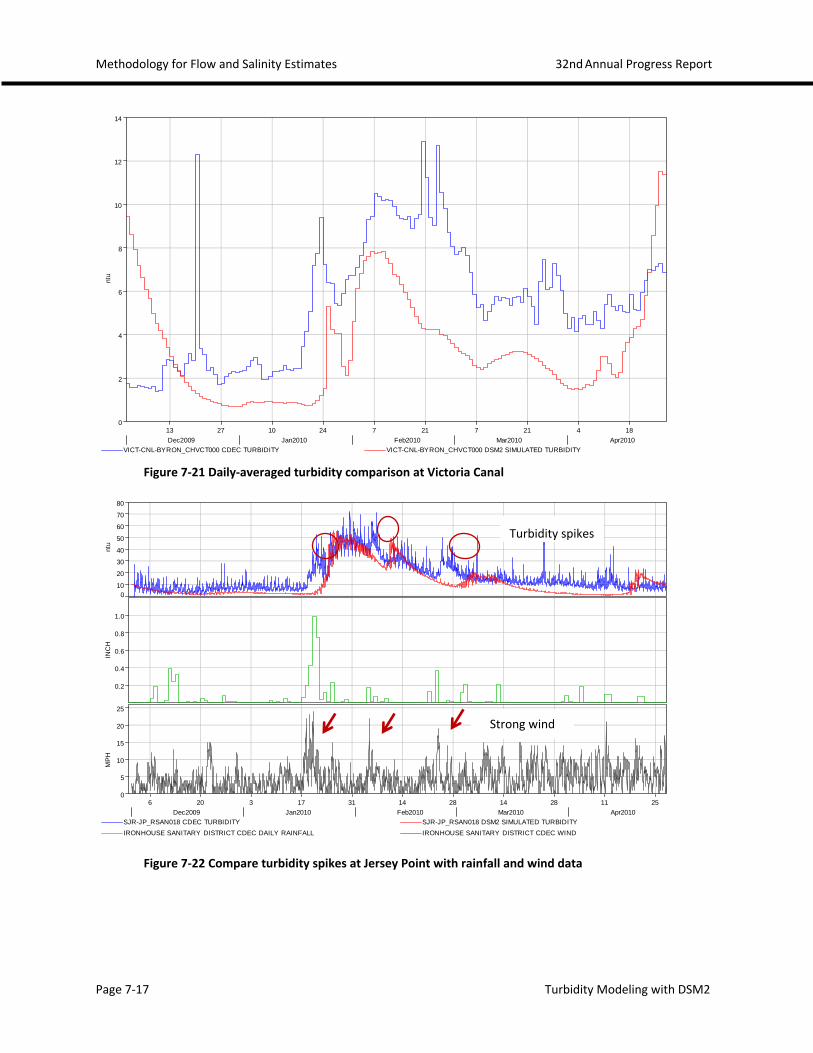
Figure 7-21 Daily-averaged turbidity comparison at Victoria Canal .................................................................... 7-17


Page 7-iv Turbidity Modeling with DSM2

Figure 7-22 Compare turbidity spikes at Jersey Point with rainfall and wind data ............................................ 7-17

Figure 7-23 Compare turbidity spikes at Bacon Island with rainfall and wind data ........................................... 7-18

Figure 7-24 Compare turbidity spikes at Holland Cut with rainfall and wind data ............................................. 7-18

Figure 7-25 Turbidity comparison at San Joaquin River Garwood ...................................................................... 7-19

Figure 7-26 Daily-averaged turbidity comparison at San Joaquin River Garwood ............................................. 7-19

Figure 7-27 Turbidity comparison at Grant Line Canal ......................................................................................... 7-20

Figure 7-28 Daily-averaged turbidity comparison at Grant Line Canal ............................................................... 7-20

Figure 7-29 Flow at San Joaquin River Mossdale (RSAN087) and Brandt Bridge (RSAN072) ............................ 7-21

Figure 7-30 Velocity at San Joaquin River Mossdale and Brandt Bridge ............................................................. 7-21

Figure 7-31 Settling rate sensitivity test result at Decker Island .......................................................................... 7-22

Figure 7-32 Settling rate sensitivity test result at Prisoners Point ....................................................................... 7-22

Figure 7-33 Settling rate sensitivity test result at Holland Cut ............................................................................. 7-23

Figure 7-34 Settling rate sensitivity test result at False River .............................................................................. 7-23

Figure 7-35 Settling rate sensitivity test result at Victoria Canal ......................................................................... 7-24

Figure 7-36 Settling rate sensitivity test result at Rough and Ready Island ........................................................ 7-24

Figure 7-37 Settling rate sensitivity test result at Grant Line Canal ..................................................................... 7-25

Figure 7-38 Daily-averaged turbidity comparison at Mallard .............................................................................. 7-25

Figure 7-39 Adjusted turbidity comparison at Mallard ........................................................................................ 7-26

Figure 7-40 Daily-averaged turbidity comparison at Antioch .............................................................................. 7-26

Figure 7-41 Adjusted turbidity comparison at Antioch ........................................................................................ 7-27

Figure 7-42 Adjusted turbidity comparison at Prisoners Point ............................................................................ 7-27

Figure 7-43 Adjusted turbidity comparison at Holland Cut ................................................................................. 7-28

Figure 7-44 Adjusted turbidity comparison at Victoria Canal .............................................................................. 7-28

Table

Table 7-1 Turbidity sources ...................................................................................................................................... 7-4


Page 7-1 Turbidity Modeling with DSM2

7 Turbidity Modeling with DSM2

7.1 Introduction This chapter documents turbidity modeling with Delta Simulation Model II (DSM2) Version 8.0.6. Turbidity has been deemed to be an important factor affecting delta smelt migration and entrainment. DSM2 is a promising tool in turbidity analysis and forecasting because of its speed as a 1-D model and its extensive applications in the Delta. A large number of stations with turbidity data became available in 2010, which makes a more detailed calibration possible for the 2010 wet season. The calibrated DSM2 model results generally match with the observed data. Further validation with another wet year will help improve its reliability.

7.2 Turbidity Modeling with DSM2 Turbidity measures the scattering effect that suspended solids have on light and is typically reported in nephelometric turbidity units (NTU): the higher the intensity of scattered light, the higher the turbidity. Material that causes water to be turbid includes (Swanson and Baldwin 2011):

• clay

• silt

• finely divided organic and inorganic matter

• soluble colored organic compounds

• plankton

• microscopic organisms

Although turbidity is not a material, it is directly related to suspended sediment concentration (SSC), and researchers found that turbidity and SSC are proportional throughout San Francisco Bay (Resource Management Associates, Inc. [RMA] 2010). It is reasonable to simulate turbidity directly with DSM2 as a constituent that is governed by advection-dispersion equation with decay/loss due to settling.

DSM2 does not have a sediment transport or turbidity component. The Carbonaceous Biochemical Oxygen Demand (BOD) function is adapted to simulate turbidity with the deoxygenation rate coefficient (K1) set to zero, and settling rate K3 calibrated to simulate the loss due to settling. The BOD function as expressed in the QUAL2E model document (Brown and Barnwell 1987) takes into account BOD removal due to sedimentation: dLdt K L K L Eq. 7-1

where

L = the concentration of ultimate carbonaceous BOD, mg/L

K1 = deoxygenation rate coefficient, day-1

K3 = the rate of loss of carbonaceous BOD due to settling, day-1



The equation for turbidity function can be written as: dTdt K T Eq. 7-2

where

T = turbidity, NTU

K3 = the rate of decrease of turbidity due to settling, day-1

7.3 Boundary Conditions The simulations used the latest Mini-Calibration historical run setup. Observed turbidity data at Hood, Vernalis, and Martinez were the main boundary conditions used (Figure 7-1)1. Observed turbidity data at Hood were shifted 12 hours to account for the travel time from upstream boundary and verified at Hood to match the observed timing (we use Hood data instead of Freeport because we had only Hood data for the 2008 winter season). The initial turbidity and agricultural drainage were set at 10 NTU. At other tributary inflows that didn’t have observed turbidity data, RMA formulas (Resource Management Associates, Inc. [RMA] 2010) were used to calculate the turbidities based on flows, including the Yolo Bypass, Mokelumne River, Cosumnes River, and Calaveras River. The total contribution from these tributaries was verified to be very small compared to Sacramento River and San Joaquin River for the calibration period of 2010. Possible errors by using the formulas should not affect the calibration much. Observed data will be used when available.

7.4 2010 Wet Season Calibration In this effort, DSM2 was calibrated on the 2010 wet season (December 2009 to April 2010). Previous studies (Chandra Chilmakuri, CH2M Hill 2010) (Resource Management Associates, Inc. [RMA] 2008 Oct) used uniform settling or decay coefficients for the entire Delta (RMA 2010 new model used 3 regions for the decay rate). In this calibration, we tried to match the observed turbidity at most of the locations by making more groups of channels by region and adjusting the settling rate in each group.

The calibration was started with a settling rate (K3) of 0.05 day-1 everywhere (as recommended by previous studies by CH2M Hill and RMA). The simulated turbidities on stations along the Sacramento River side were satisfactory. We adjusted the settling rates on the San Joaquin, Old, and Middle Rivers to get the simulated turbidity close to the field data. Altogether, 10 groups (5 distinct values) were used as shown in the map of Figure 7-2.

The results were mainly compared by visual inspection. Due to the model limitations (discussed later), big differences occur in some locations and time periods due to local storm events and other factors. By visual comparison, it is easy to ignore differences due to local storm events and pay attention to the general trend and peak values.

A complete comparison report at all stations was generated using the newly developed DSM2 report tool (Hsu 2010). This tool was a tremendous help in calibration because numerous runs were made to

1 All figures appear at the back of this chapter



test the sensitivity of result output to parameters. It made it feasible to plot the results after every run. Final results are plotted with HEC-DSSVUE and pasted here for discussion.

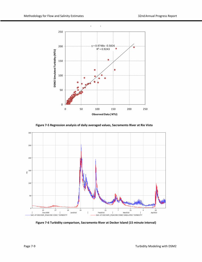
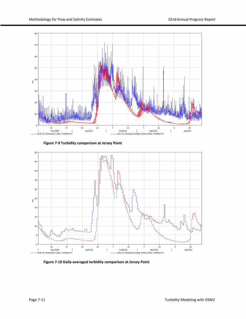
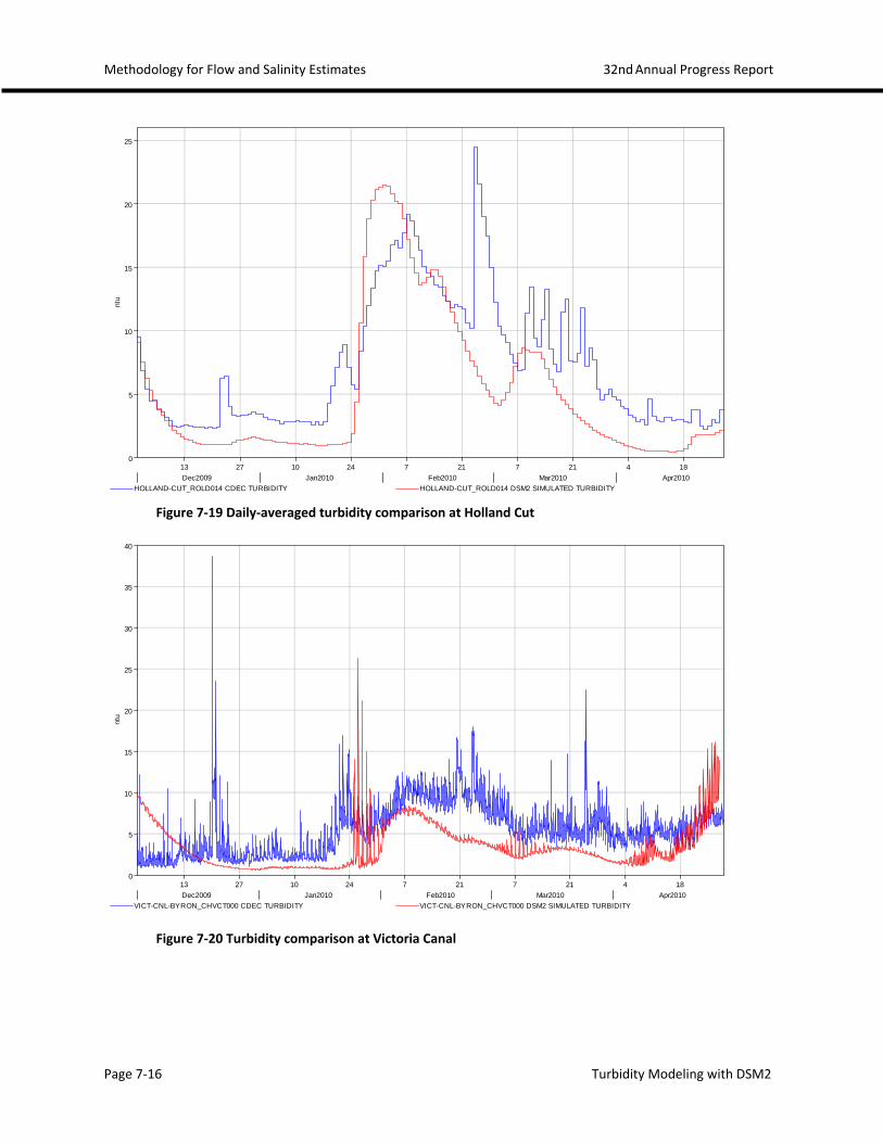
The simulated results compare well with field data along the Sacramento River, as seen at Rio Vista and Decker Island (Figure 7-3 to Figure 7-8). At central and south Delta, the general trends compare well as seen at Jersey Point, Prisoners Point, Holland Cut, Bacon Island, Victoria Canal (Figure 7-9 to Figure 7-21). Some turbidity spikes shown in field data but not seen in the modeling results are due to local storm events and can be verified to be co-related with rainfall and wind data, as shown in Figure 7-22 Figure 7-24. Figure 22 shows strong winds are associated with the turbidity spikes at Jersey Point.

Very large settling rates were used for San Joaquin River from Mossdale to Garwood (0.7 day-1) and Old River upstream of Clifton Court Forebay and Grant Line Canal (0.5 day-1) in order to bring down the turbidity to field observed levels (Figure 7-25 to Figure 7-28). One reason to justify the bigger values at these reaches is that the rivers just enter tidal influence zone. Flood tides cause flow to slow down to zero velocity and even reverse direction, and cause rapid sediment settling. As seen in Figure 7-29, the flow patterns at Mossdale (RSAN087) and Brandt Bridge (RSAN072) are quite different. The flow velocity at Mossdale is always positive, but at Brandt Bridge velocity goes to zero and negative during flood tides (Figure 7-30). Other reasons may include additional dilution due to missing tributary inflows as discussed in RMA report (2010).

Figure 7-31 to Figure 7-37 show sensitivity test results by increasing and decreasing the calibrated settling rates (K3) 50%. Along the Sacramento River, the settling rate was very small and not very sensitive to the change, as seen at Decker Island (Figure 7-31). At central Delta stations, the results are very sensitive to the changes, as seen in plots of Prisoners Point, Holland Cut, False River, and Victoria Canal (Figure 7-32 to Figure 7-35). Figure 7-36 and Figure 7-37 show the sensitivity test at San Joaquin River at Rough and Ready Island and Grant Line Canal. It can be seen that lower settling rates would result in the simulated turbidity peaks being too high.

7.5 Discussion of Model limitations The settling rate in DSM2 model is essentially the same as using first order decay rate as used by RMA (2010). RMA (2010) discussed limitations of the simple modeling approach. Similar to RMA modeling, there are several mechanisms affecting turbidity but not reflected in the DSM2 modeling:

• The model does not have the mechanism of sediment re-suspension. It will not calculate turbidity created by wave/current caused by wind and tide.

• The settling rate should be co-related to flow velocity and suspended sediment properties. Instead, it is calibrated only on locations.

• Discrepancies between the model results and field data can be contributed also to in-Delta precipitation, missing runoff/inflow, etc. It can be seen in the comparison plots that big discrepancies occur during local rainfall/storm events (Figure 7-22 to Figure 7-24)



The sources of turbidity can be categorized and summarized in Table 7-1.

Table 7-1 Turbidity sources

Source Included in model Comments

Turbidity from boundaries

Main boundaries: Sacramento, San Joaquin, Martinez;

Tributaries: Yolo Bypass, Mokelumne River, Cosumnes River, Calaveras River.

Transport and settling are modeled. Results match the general trend and magnitude well.

Local storm contributions

No Turbidity spikes can be seen in the field data due to local storms (runoff, wave/current re-suspension by strong storm wind). Big differences can be seen when comparing modeling results with field data. The monthly averaged DICU input cannot reflect the flows during storm events.

Re-suspension by normal wave/current

No This is the main source of turbidity under normal conditions (when there are no storm events) besides turbidity transported from boundaries. An ad hoc procedure is proposed to compensate this effect in the model results.

The observed turbidity values at west Delta stations (Mallard, Antioch) are always much higher than in central Delta/south Delta under normal conditions (before any significant storm occurs in December or January). This may be contributed to re-suspension by stronger wind wave and tidal current effects in west Delta.

The model simulates turbidity using one settling rate at each location. The different types of sediment and materials are not considered separately. The model is calibrated during big events, the calibrated settling rate may reflect more coarse sediment, and may not reflect the finer or lighter materials under normal conditions well, i.e., the calibrated settling rates may tend to be high under normal conditions and cause more settling during the normal condition period.

Due to these limitations, the model does not simulate the turbidity well under normal conditions. The shortcomings are more obvious in west Delta than in south Delta. It can be seen in Figure 7-38 and Figure 7-40, the model could not match the observed turbidity at Mallard and Antioch in December and early January, as highlighted in the figures. At south Delta, the wind wave effect is smaller, and turbidities are usually less than 5 NTU.

The simulated turbidity may be adjusted for the missing re-suspension mechanism when comparing with field data, especially at west Delta stations. In Figure 7-39, the simulated turbidity at Mallard was adjusted by adding 11.0 NTU (the smallest difference between observed and simulated turbidity in late December and early January). This adjustment eliminates the differences under normal



conditions and may improve prediction. In Figure 7-41, the simulated turbidity at Antioch was adjusted by adding 8.0 NTU (the smallest difference between observed and simulated turbidity in late December and early January). Figure 7-42 to Figure 7-44 show the adjusted turbidity comparison at Prisoners Point (adjusted 3.0 NTU), Holland Cut (adjusted 1.5 NTU), and Victoria Canal (adjusted 1.0 NTU). These 3 stations were used in the US Fish and Wildlife Service (USFWS) Delta Smelt Biological Opinion (December 15, 2008) as a trigger in the Reasonable and Prudent Alternative action (3-day average is greater than or equal to 12 NTU at these stations). Although the differences adjusted are very small at these stations, the adjustment helps improve the comparison and accuracy of the modeled turbidity.

7.6 Summary

DSM2 can be adapted to simulate transport and settling of turbidity in the Delta. Factors, such as local storm runoff/inflow, wave/current re-suspension, were not modeled. Despite the limitations, the calibrated model generally simulated the main turbidity events well. The comparison of simulated turbidity and field data are convincing. A validation of another wet year will give more confidence in the model calibration.

Further improvements are desirable to incorporate re-suspension and local storm runoff/inflow effects, but these improvements may require much greater efforts and are beyond the scope of this study. A simple ad hoc adjustment is proposed to compensate wave/current re-suspension effect, and help improve model accuracy.

7.7 Acknowledgments

Marianne Guerin (of Resource Management Associates, Inc.) provided quality-checked 2010 turbidity data; Siqing Liu (of DWR) updated the historical run to 2010.

7.8 References Brown, Linfield C., and Jr., Thomas O. Barnwell. "The Enhanced Stream Water Quality Models QUAL2E and

QUAL2E-UNCAS: Documentation and User Manual." 1987.

Chandra Chilmakuri, CH2M Hill. Turbidity Simulation in the Delta using DSM2. Sacramento: DSM2UG Newsletter, DWR, 2010.

Hsu, En-Ching. "Chapter 10: DSM2 Comparison Report Tool." Methodology for Flow and Salinity Estimates in the Sacramento-San Joaquin Delta and Suisun Marsh. 32nd Annual Progress Report from the California Department of Water Resources to the State Water Resources Control Board, 2010.

Resource Management Associates, Inc. [RMA]. Near-Real-time Turbidity and Adult Delta Smelt Forecasting with RMA 2-D Models (draft). Fairfield, California: Prepared for the Metropolitan Water District of Southern California, 2010.

Resource Management Associates, Inc. [RMA]. Sacramento-San Joaquin Delta Turbidity Modeling. Appendix A Technical Memorandum, Fairfield, California: Prepared for the Metropolitan Water District of Southern California, 2008 Oct.

Swanson, H. A., and H. L. Baldwin. Information on this page is from "A Primer on Water Quality", U.S. Geological Survey, 1965. Feb 8, 2011. http://ga.water.usgs.gov/edu/characteristics.html.



Note: Stations discussed in this chapter are highlighted

Figure 7-1 CDEC turbidity stations



Figure 7-2 Calibrated settling rate values



Figure 7-3 Turbidity comparison, Sacramento River at Rio Vista (15 minute interval)

Figure 7-4 Daily-averaged turbidity comparison, Sacramento River at Rio Vista

13 27 10 24 7 21 7 21 4 18Dec2009 Jan2010 Feb2010 Mar2010 Apr2010

ntu

-50

0

50

100

150

200

250

300

RIO-VISTA_RSAC101 CDEC TURBIDITY RIO-VISTA_RSAC101 DSM2 SIMULATED TURBIDITY


ntu

0

50

100

150

200

RIO-VISTA_RSAC101 CDEC TURBIDITY RIO-VISTA_RSAC101 DSM2 SIMULATED TURBIDITY



Figure 7-5 Regression analysis of daily averaged values, Sacramento River at Rio Vista

Figure 7-6 Turbidity comparison, Sacramento River at Decker Island (15 minute interval)


ntu

0

50

100

150

200

250

300

SAC-AT-DECKER_RSAC092 CDEC TURBIDITY SAC-AT-DECKER_RSAC092 DSM2 SIMULATED TURBIDITY

y = 0.9748x - 0.5826R² = 0.9243

0

50

100

150

200

250

0 50 100 150 200 250

DSM

2 Si

mul

ated

Tur

bidi

ty (N

TU)

Observed Data ( NTU)

y p



Figure 7-7 Daily-averaged turbidity comparison, Sacramento River at Decker Island

Figure 7-8 Regression analysis of modeled result and field data, Sacramento River at Decker Island


ntu

0

20

40

60

80

100

120

140

160

180

200

SAC-AT-DECKER_RSAC092 CDEC TURBIDITY SAC-AT-DECKER_RSAC092 DSM2 SIMULATED TURBIDITY

y = 0.9988x - 5.3842R² = 0.944

0

50

100

150

200

0 50 100 150 200

DSM

2 Si

mul

ated

Tur

bidi

ty (N

TU)




Figure 7-9 Turbidity comparison at Jersey Point

Figure 7-10 Daily-averaged turbidity comparison at Jersey Point


ntu

0

10

20

30

40

50

60

70

80

SJR-JP_RSAN018 CDEC TURBIDITY SJR-JP_RSAN018 DSM2 SIMULATED TURBIDITY


ntu

0

5

10

15

20

25

30

35

40

45

50

SJR-JP_RSAN018 CDEC TURBIDITY SJR-JP_RSAN018 DSM2 SIMULATED TURBIDITY



Figure 7-11 Regression analysis of modeled result and field data at Jersey Point

Figure 7-12 Turbidity comparison at Old River Bacon Island


ntu

0

5

10

15

20

OLD-R-BACON_ROLD024 CDEC TURBIDITY OLD-R-BACON_ROLD024 DSM2 SIMULATED TURBIDITY

y = 0.9401x - 3.6984R² = 0.7731

0

10

20

30

40

50

60

0 10 20 30 40 50 60

DSM

2 Si

mul

ated

Tur

bidi

ty (N

TU)




Figure 7-13 Daily-averaged turbidity comparison at Old River Bacon Island

Figure 7-14 Regression analysis of modeled result and field data at Old River Bacon Island


ntu

0

2

4

6

8

10

12

14

16

18

20

OLD-R-BACON_ROLD024 CDEC TURBIDITY OLD-R-BACON_ROLD024 DSM2 SIMULATED TURBIDITY

y = 0.9756x - 1.5823R² = 0.6443

0

2

4

6

8

10

12

14

16

18

20

0 5 10 15 20

DSM

2 Si

mul

ated

Tur

bidi

ty (N

TU)




d

Figure 7-15 Turbidity comparison, Sacramento River at Prisoners Point

Figure 7-16 Daily-averaged turbidity comparison, Sacramento River at Prisoners Point


ntu

0

10

20

30

40

50

60

70

80

PRISONER-PT_RSAN037 CDEC TURBIDITY PRISONER-PT_RSAN037 DSM2 SIMULATED TURBIDITY


ntu

0

5

10

15

20

25

30

35

40

45

PRISONER-PT_RSAN037 CDEC TURBIDITY PRISONER-PT_RSAN037 DSM2 SIMULATED TURBIDITY



Figure 7-17 Regression analysis of modeled result and field data at Prisoners Point

Figure 7-18 Turbidity comparison, Sacramento River at Holland Cut


ntu

0

10

20

30

40

50

60

70

80

HOLLAND-CUT_ROLD014 CDEC TURBIDITY HOLLAND-CUT_ROLD014 DSM2 SIMULATED TURBIDITY

y = 0.7975x - 0.7915R² = 0.8819

0

10

20

30

40

50

0 10 20 30 40 50

DSM

2 Si

mul

ated

Tur

bidi

ty (N

TU)




Figure 7-19 Daily-averaged turbidity comparison at Holland Cut

Figure 7-20 Turbidity comparison at Victoria Canal


ntu

0

5

10

15

20

25

HOLLAND-CUT_ROLD014 CDEC TURBIDITY HOLLAND-CUT_ROLD014 DSM2 SIMULATED TURBIDITY


ntu

0

5

10

15

20

25

30

35

40

VICT-CNL-BYRON_CHVCT000 CDEC TURBIDITY VICT-CNL-BYRON_CHVCT000 DSM2 SIMULATED TURBIDITY



Figure 7-21 Daily-averaged turbidity comparison at Victoria Canal

Figure 7-22 Compare turbidity spikes at Jersey Point with rainfall and wind data


ntu

0

2

4

6

8

10

12

14

VICT-CNL-BYRON_CHVCT000 CDEC TURBIDITY VICT-CNL-BYRON_CHVCT000 DSM2 SIMULATED TURBIDITY

ntu

010

20

30

40

50

60

70

80

INC

H

0.2

0.4

0.6

0.8

1.0

6 20 3 17 31 14 28 14 28 11 25Dec2009 Jan2010 Feb2010 Mar2010 Apr2010

MPH

0

5

10

15

20

25

SJR-JP_RSAN018 CDEC TURBIDITY SJR-JP_RSAN018 DSM2 SIMULATED TURBIDITYIRONHOUSE SANITARY DISTRICT CDEC DAILY RAINFALL IRONHOUSE SANITARY DISTRICT CDEC WIND

Strong wind

Turbidity spikes



Figure 7-23 Compare turbidity spikes at Bacon Island with rainfall and wind data

Figure 7-24 Compare turbidity spikes at Holland Cut with rainfall and wind data

ntu

0

5

10

15

20

INC

H

0.2

0.4

0.6

0.8

1.0


MPH

0

5

10

15

20

25

OLD-R-BACON_ROLD024 CDEC TURBIDITY OLD-R-BACON_ROLD024 DSM2 SIMULATED TURBIDITYIRONHOUSE SANITARY DISTRICT CDEC DAILY RAINFALL IRONHOUSE SANITARY DISTRICT CDEC WIND

ntu

010

20

30

40

50

60

70

80

INC

H

0.2

0.4

0.6

0.8

1.0


MP

H

0

5

10

15

20

25

HOLLAND-CUT_ROLD014 CDEC TURBIDITY HOLLAND-CUT_ROLD014 DSM2 SIMULATED TURBIDITYIRONHOUSE SANITARY DISTRICT CDEC DAILY RAINFALL IRONHOUSE SANITARY DISTRICT CDEC WIND



Figure 7-25 Turbidity comparison at San Joaquin River Garwood

Figure 7-26 Daily-averaged turbidity comparison at San Joaquin River Garwood


ntu

0

50

100

150

200

SJR-GARWOOD_CH14 CDEC TURBIDITY SJR-GARWOOD_CH14 DSM2 SIMULATED TURBIDITY


ntu

-20

0

20

40

60

80

100

120

140

160

180

SJR-GARWOOD_CH14 CDEC TURBIDITY SJR-GARWOOD_CH14 DSM2 SIMULATED TURBIDITY



Figure 7-27 Turbidity comparison at Grant Line Canal

Figure 7-28 Daily-averaged turbidity comparison at Grant Line Canal


ntu

0

20

40

60

80

100

120

140

160

180

200

GRANT-LINE_CH213 CDEC TURBIDITY GRANT-LINE_CH213 DSM2 SIMULATED TURBIDITY


ntu

0

20

40

60

80

100

120

GRANT-LINE_CH213 CDEC TURBIDITY GRANT-LINE_CH213 DSM2 SIMULATED TURBIDITY



Figure 7-29 Flow at San Joaquin River Mossdale (RSAN087) and Brandt Bridge (RSAN072)

Figure 7-30 Velocity at San Joaquin River Mossdale and Brandt Bridge


Flow

(cfs

)

-3,000

-2,000

-1,000

0

1,000

2,000

3,000

4,000

5,000

6,000

RSAN072 HIST_MINI_CALIB_V805 FLOW RSAN087 HIST_MINI_CALIB_V805 FLOW


FT/S

-1.5

-1.0

-0.5

0.0

0.5

1.0

1.5

2.0

2.5

RSAN072 HIST_MINI_CALIB_V805 VEL RSAN087 HIST_MINI_CALIB_V805 VEL



Figure 7-31 Settling rate sensitivity test result at Decker Island

Figure 7-32 Settling rate sensitivity test result at Prisoners Point


ntu

-0

20

40

60

80

100

120

140

160

180

200

SAC-AT-DECKER_RSAC092 CDEC TURBIDITY SAC-AT-DECKER_RSAC092 DSM2 SIMULATED TURBIDITYSAC-AT-DECKER_RSAC092 SETTLING RATE +50% TURBIDITY SAC-AT-DECKER_RSAC092 SETTLING RATE -50% TURBIDITY


ntu

-0

5

10

15

20

25

30

35

40

45

50

PRISONER-PT_RSAN037 CDEC TURBIDITY PRISONER-PT_RSAN037 DSM2 SIMULATED TURBIDITYPRISONER-PT_RSAN037 SETTLING RATE +50% TURBIDITY PRISONER-PT_RSAN037 SETTLING RATE -50% TURBIDITY



Figure 7-33 Settling rate sensitivity test result at Holland Cut

Figure 7-34 Settling rate sensitivity test result at False River


ntu

0

5

10

15

20

25

30

35

40

HOLLAND-CUT_ROLD014 CDEC TURBIDITY HOLLAND-CUT_ROLD014 DSM2 SIMULATED TURBIDITYHOLLAND-CUT_ROLD014 SETTLING RATE +50% TURBIDITY HOLLAND-CUT_ROLD014 SETTLING RATE -50% TURBIDITY


ntu

0

10

20

30

40

50

60

FALSE_R CDEC TURBIDITY FALSE_R DSM2 SIMULATED TURBIDITY FALSE_R SETTLING RATE +50% TURBIDITYFALSE_R SETTLING RATE -50% TURBIDITY



Figure 7-35 Settling rate sensitivity test result at Victoria Canal

Figure 7-36 Settling rate sensitivity test result at Rough and Ready Island


ntu

0

5

10

15

20

VICT-CNL-BYRON_CHVCT000 CDEC TURBIDITY VICT-CNL-BYRON_CHVCT000 DSM2 SIMULATED TURBIDITYVICT-CNL-BYRON_CHVCT000 SETTLING RATE +50% TURBIDITY VICT-CNL-BYRON_CHVCT000 SETTLING RATE -50% TURBIDITY


ntu

0

20

40

60

80

100

120

140

160

ROUGH-N-READY_RSAN058 CDEC TURBIDITY ROUGH-N-READY_RSAN058 DSM2 SIMULATED TURBIDITYROUGH-N-READY_RSAN058 SETTLING RATE +50% TURBIDITY ROUGH-N-READY_RSAN058 SETTLING RATE -50% TURBIDITY



Figure 7-37 Settling rate sensitivity test result at Grant Line Canal

Figure 7-38 Daily-averaged turbidity comparison at Mallard


ntu

0

20

40

60

80

100

120

140

160

180

GRANT-LINE_CH213 CDEC TURBIDITY GRANT-LINE_CH213 DSM2 SIMULATED TURBIDITYGRANT-LINE_CH213 SETTLING RATE +50% TURBIDITY GRANT-LINE_CH213 SETTLING RATE -50% TURBIDITY


ntu

0

20

40

60

80

100

120

140

160

MALLARD-SL_RSAC075 CDEC TURBIDITY MALLARD-SL_RSAC075 DSM2 SIMULATED TURBIDITY

Big difference under normal condition




Figure 7-39 Adjusted turbidity comparison at Mallard

Figure 7-40 Daily-averaged turbidity comparison at Antioch


ntu

0

20

40

60

80

100

120

140

160

MALLARD-SL_RSAC075 CDEC TURBIDITY MALLARD-SL_RSAC075 DSM2 SIMULATED-ADJUSTED TURBIDITY


ntu

0

10

20

30

40

50

60

70

80

ANTIOCH_RSAN007 CDEC TURBIDITY ANTIOCH_RSAN007 DSM2 SIMULATED TURBIDITY




Figure 7-41 Adjusted turbidity comparison at Antioch

Figure 7-42 Adjusted turbidity comparison at Prisoners Point


ntu

0

10

20

30

40

50

60

70

80

90

ANTIOCH_RSAN007 CDEC TURBIDITY ANTIOCH_RSAN007 DSM2 SIMULATED-ADJUSTED TURBIDITY


ntu

0

5

10

15

20

25

30

35

40

45

PRISONER-PT_RSAN037 CDEC TURBIDITY PRISONER-PT_RSAN037 DSM2 SIMULATED_ADJUSTED TURBIDITY



Figure 7-43 Adjusted turbidity comparison at Holland Cut

Figure 7-44 Adjusted turbidity comparison at Victoria Canal


ntu

0

5

10

15

20

25

HOLLAND-CUT_ROLD014 CDEC TURBIDITY HOLLAND-CUT_ROLD014 DSM2 SIMULATED_ADJUSTED TURBIDITY


ntu

0

2

4

6

8

10

12

14

VICT-CNL-BYRON_CHVCT000 CDEC TURBIDITY VICT-CNL-BYRON_CHVCT000 DSM2 SIMULATED_ADJUSTED TURBIDITY

Documents

Chapter 7 Turbidity Modeling with DSM2 - Californiabaydeltaoffice.water.ca.gov/modeling/deltamodeling/AR2011/Method... · Chapter 7 Turbidity Modeling with DSM2 ... 7-12 Figure 7-12