Embed Size (px)
Citation preview

CHAPTER 8
‘Dead’ recovery models
The first chapters in this book focussed exclusively on live encounter ‘mark-recapture’ models,where the
probability of an individual being seen (encountered) on a particular sampling occasion was determined
by 2 parameters: the probability the animal survived and the probability that an animal alive in state r
at time i is alive and in state s at time i+1.
In this chapter, we move in a new direction altogether. We recall that ‘classic’ mark-recapture focuses
on the problem of differentiating between (i) not seeing an animal because it is ‘dead’ (or permanently
emigrated from the sample area) and (ii) simply ‘missing’ it, even though it is alive and in the sample
area. In contrast, with ‘dead recovery’ analysis we are dealing with animals known to be dead (because
they are recovered in the ‘dead state’, frequently in the process of harvest).
Echoing the seminal text by Brownie et al. (1985), it is sufficiently important to clearly distinguish
between these two broad classes of sampling method (recovery and recapture) that we’ll take a moment
to elaborate on them. In the case of a recapture analysis, a single marked individual is potentially
available for ‘multiple encounters’ – i.e., the individual may be ‘seen’ or ‘recaptured’ on more than one
occasion. If you’ve worked through the preceding chapters of this book, this is entirely obvious to you.
In contrast, in a recovery analysis, data are available on only a single, terminal ‘encounter’ (generally, the
recovery event). Unlike recapture data, recovery data are treated as independent, mutually exclusive
outcomes (i.e., a marked individual could be recovered in year 1, year 2, or not at all during the duration
of the study). While this is a clear difference from a live encounter study, in fact, close examination shows
deep similarity between the two models. The distribution of ‘dead recoveries’ reflects the realization
of a series of probabilistic events. Just as each live encounter in a live encounter history reflects the
underlying survival and encounter processes, so too does the distribution of ‘dead recoveries’.
8.1. ‘Brownie’ parameterization
Consider the following example. An individual of a harvested species is marked and released alive.
This newly marked individual can then experience one of 3 fates: (1) it can survive the year with
some probability, (2) it can be ‘harvested’ (i.e., some ‘action’ leading to permanent removal) with some
probability, or (3) it can ‘die’ from ‘natural’ causes (i.e., it might actually die from some reason other
than harvest, or permanently emigrate the sampling area, at which point it appears dead. More on what
constitutes the ‘sampling area’ for a dead recovery analysis in Chapter 9).
However, before this individual becomes ‘dead recovery data’, something else needs to happen –
the ‘harvest’ needs to be ‘reported’. This event reflects several underlying probabilistic events. Suppose
you’re a waterfowl hunter, and you shoot a bird from your blind (or ‘hide’ for much of the world). This
© Cooch & White (2018) 03.14.2018

8.1. ‘Brownie’ parameterization 8 - 2
in itself does not constitute a recovery, since simply shooting the bird does not give us the information
on who it is (i.e., its identification number). For this to happen, minimally (in most cases), the marked
bird needs to be retrieved (i.e., physically handled, typically). Of course, there is some chance it won’t be
retrieved. If it is retrieved, however, then it might be ‘reported’ (i.e., the identification number submitted
to some monitoring agency), or not. We’ll let S equal the probability that the individual survives the year.
We separate sources of mortality into ‘hunter’ and ‘natural’. The probability that the individual dies
from either source is simply 1− S. The probability that it dies due to hunting is K. Thus, the probability
that it dies from natural causes is (1 − S − K).
Now for the only real complication (that is simple enough in principle, but has several interesting
implications we will discuss later in this chapter). Conditional on being shot (i.e., killed by hunting, with
probability K), then one of 3 things can happen. The individual may not be retrieved (a fairly common
occurrence with some types of harvest – individuals are in fact killed by harvest, but the dead animal
is not physically retrieved). The probability of being retrieved is c – thus, the probability of not being
retrieved is (1 − c). Conditional upon being retrieved, the hunter can either report the identification
number (with probability λ), or not report the identification number (with probability 1 − λ).
Let’s put these probabilities together, using a ‘fate diagram’ (following Brownie et al. 1985).
Thus, recovery data supplies information directly (and directly is the key operative word here) about
only those birds which are shot and reported. Thus, under this parameterization, not everything is
estimable – only the product Kcλ is estimable, but the component probabilities K, c and λ are not.
Generally, the product Kcλ (often written as Hλ, where H � Kc = harvest rate; the probability of being
killed and retrieved by a hunter during the year) is referred to as the recovery rate, f.∗ Using these
‘product’ (summary) parameters, we can modify the preceding ‘fate diagram’ as follows:
Different assumptions about the parameters f and S give rise to the different models. In this sense,
you can loosely (very loosely) think of f and S as the equivalents of p and ϕ for a live recapture analysis –
∗ We note that neither ‘harvest rate’ or ‘recovery rate’ are ‘rates’ in the strict sense of the word (which implies instantaneousrates of change). Strictly speaking, they should be referred to as ‘harvest probability’ and ‘recovery probability’, respectively.However, the use of the word ‘rate’ is traditional for these models.
Chapter 8. ‘Dead’ recovery models

8.1. ‘Brownie’ parameterization 8 - 3
clearly not in terms of what they represent, but in the fact that the ‘encounter history’ is defined by these
2 probabilities. Remember, the components of the recovery probability f (i.e., Kcλ) are not estimable
without additional information (discussed later).
Let’s see how these two primary parameters (f and S) combine to determine the expected numbers
of bands recovered in a particular time period. The process is analogous to expressing the expected
numbers of individuals with capture history ‘101101’ as a function of the number released (R) and the
underlying survival and recapture probabilities.
Suppose N1 individuals are marked. How many recoveries are expected during the next year? Note,
we’re not asking specifically how many individuals are alive at the end of the 12 months following
marking (although this can be derived, obviously), but rather, how many individuals will be (i) shot by
hunters, (ii) retrieved,and (iii) reported?Look at the fate diagram on the preceding page. The probability
that an individual is harvested, retrieved and reported (i.e., theindividual is recovered) is simply f. Thus,
the expected number of the N1 released individuals we expect to be recovered in the first interval after
marking is given simply as N1 f .
If we assume for the moment that both survival and recovery probabilities are time-specific, then the
expected number of recoveries are given as follows:
year recovered
year marked number marked 1 2 3 l � 4
1 N1 N1 f1 N1S1 f2 N1S1S2 f3 N1S1S2S3 f4
2 N2 N2 f2 N2S2 f3 N2S2S3 f4
3 N3 N3 f3 N3S3 f4
k � 4 N4 N4 f4
Make sure you understand the connection between f, S, and the expected number of recoveries. Si is
the probability of surviving from time (i − 1) to time (i), whereas f (recovery rate) is the probability of
being shot (i.e., not surviving), and then being retrieved and reported. So, f (recovery rate) combines the
mortality event with two other events (retrieval and reporting). For example, for individuals marked in
year 1, the number of expected dead recoveries in the second interval after marking is given as N1S1 f2.
Why? Well, recall that the recovery parameter f is the probability of the mortality event. In order for
the individual to be a dead recovery in the second interval, it has to survive the first interval (with
probability S1), and then be harvested, retrieved and reported (with probability f2). Note that survival
S does not appear on the diagonal.
Now, if you’ve already worked through the earlier chapters on mark-recapture, in looking at the table
of expected number of recoveries (above), you probably recognize right away that there are reduced
parameter models which can be fit. The expected recoveries shown in the preceding table reflect
the expectations from a time-dependent model {St ft }. Of course, you could fit model {St f·} – time
dependence in survival only, or model {S· f·} – constant survival and recovery probabilities, or a whole
host of additional models. For the moment, let’s quickly run through how you would fit the following
4 models: {St ft}, {S· ft }, {St f·} and {S· f·}.
Historically, a subset of these models have been referred to by generic model names (for example,
model {St ft} is referred to in Brownie et al. (1985) as Model 1). In the following, we note this historical
connection – we suggest that in general you use a explicit model naming convention as we’ve used
throughout the book (and as suggested in Lebreton et al. 1992). However, it is important to understand
the historical naming conventions to allow you to easily read and interpret earlier papers and texts.
Chapter 8. ‘Dead’ recovery models

8.1. ‘Brownie’ parameterization 8 - 4
For individuals marked as adults, our models (and their corresponding legacy names) are:
model legacy name reference
{St ft } Model 1 Brownie et al. (1985) pp. 15-20
{St f·} none
{S· ft} Model 2 Brownie et al. (1985) pp. 20-24
{S· f·} Model 3 Brownie et al. (1985) pp. 24-30
You might be wondering about model {St f·}? There is no corresponding model in Brownie et al.
(1985) because this model (which assumes the recovery probability f is constant over time, while
survival S varies) is seldom applicable to the waterfowl data sets for which the model set in Brownie et
al. (1985) was developed.
To demonstrate how to fit these models using MARK, we’ll use data set BROWNADT.INP (a subset of the
BROWNIE.INP data file distributed with MARK). BROWNADT.INP contains the recovery data for adult male
mallards marked in the San Luis Valley in Colorado, from 1963 to 1971. The full data set (BROWNIE.INP)
contains data for both the adults and juveniles. For the moment, we’ll look only at the adults.
Start MARK, and begin a new project by pulling down the ‘File’ menu and selecting ‘New’. Select
the file BROWNADT.INP. Before we go any further, let’s have a look at the file. Again, the easiest way to do
this is to click the ‘View file’ button. Here’s what BROWNADT.INP looks like:
We see that the data are stored in ‘classic’ recovery matrix form. It is not necessary to format the data
this way for a recovery analysis, but it is a traditional summary format. However, remember that using
any sort of summary format, whether for a recovery analysis or for (say) mark-recapture analyses has
the major disadvantage of not allowing individual covariates (since all individuals are lumped together
in the summary). The other approach is to use the familiar encounter history format. MARK makes
use of what we refer to as the ‘LDLD’ format to code dead recovery data (and joint live encounter-dead
recovery data – this data type is covered in chapter 9). For more details on the LDLD data format, see
Chapter 2.
There are 9 ‘sampling occasions’ in this data set, although we submit that occasions is not particularly
useful as a reference term, since it is not accurate. In mark-recapture, the occasion is used to refer to the
point in time (i.e, the sampling occasion) upon which a marked individual was encountered. Occasions
were separated by intervals. In recovery analysis, the data refer to the total number of individuals
recovered during the interval, and not at a particular occasion.
Chapter 8. ‘Dead’ recovery models

8.1. ‘Brownie’ parameterization 8 - 5
Consider the following diagram – individuals are initially marked and live released at (say) occasion
1,but are not encountered alive at any subsequent sampling occasion (2, 3,...). All subsequent encounters
of individuals marked and live released at occasion 1 are encountered – once – as a dead recovery, in
either period 1 (i.e., interval between occasion 1 and 2), period 2 (interval between occasion 2 and 3),
and so on.
1 2 3
(initial live release)
occasion 1 occasion 2 occasion 3
dead encounters dead encounters
Thus, for dead recovery analysis, it is more appropriate to refer to the intervals themselves. In this
example, we have 9 years (l � 9) of recovery data (as it turns out, ranging from 1963 to 1971). The
bottom row indicates the number of newly marked individuals released at the start of each year (note
that the year doesn’t necessarily start with January 1 – it could be that ‘year’ refers to the 12-month
interval between hunting seasons, for example). So, at the start of what we refer to as 1963, 231 newly
marked adult mallards were released. Of these, 10 were recovered during the first 12 months following
this release, 13 were recovered the next year, and so forth. Birds were marked and released each year
of the study – in other words, there are k � 9 rows of recovery data in the data file (i.e., the recovery
matrix is symmetric, k � l). This becomes important later on, so keep the fact that ‘k � l’ in the back of
your mind. Set the number of encounter occasions in MARK to 9.
Now we need to select the data type. Remember, MARK ‘can’t tell’ the sort of data (or analysis)
you are interested in from the data – you have to ‘tell it’. Now, if you look at the data type list in the
MARK specification window, you’ll see a radio-button corresponding to ‘Dead Recoveries’. If you
select this radio-button, a small window will pop up as you to pick a dead recovery data type. Three are
listed: ‘Dead Recoveries (Seber)’, ‘Dead Recoveries (Brownie et al.)’, and ‘BTO Dead Recoveries
and Unknown Ringings’.
We’re starting with the ‘Brownie’ approach, even though it is not the first one presented in the MARK
data type menu,simply because it is the ‘classic’ approachused in the vastmajority ofpublishedrecovery
analysis. So, as shown, select the ‘Dead Recoveries (Brownie et al.)’ data type from the list, and then
click the ‘OK’ button. You should now see the survival (S) PIM on the screen (just as with live encounter
– recapture – data, MARK defaults to opening up the ‘survival’ PIM). However, there are some subtle
but important differences between the survival and recovery PIMs, at least when using the Brownie
parameterization. To explore this, let’s also open up the recovery (f ) PIM for comparison.
Chapter 8. ‘Dead’ recovery models

8.1. ‘Brownie’ parameterization 8 - 6
Woah – wait a second! These two PIMs don’t have the same number of rows and columns – is this
a mistake?! No! This is exactly the way it should be. Of course, now you need to consider why this is
true. Look again at the table of expected recoveries, and the associated probability expressions – below
(here, we are considering only 4 years (l � k � 4), but the principle is exactly the same):
year recovered
year marked number marked 1 2 3 l � 4
1 N1 N1 f1 N1S1 f2 N1S1S2 f3 N1S1S2S3 f4
2 N2 N2 f2 N2S2 f3 N2S2S3 f4
3 N3 N3 f3 N3S3 f4
k � 4 N4 N4 f4
The key is to look carefully at the probability expressions in each cell. Remember that in the case of
live mark-recapture, the PIMs are (in effect) constructed from the subscripts of the parameters in the
corresponding probability expressions. What about for dead recovery analysis? Look at the subscripting
of the two primary parameters, S and f. If you look along the first row (the row with the greatest number
of columns – years), we see that the subscripting for recovery probability f ranges from ‘1’ to ‘4’. In
contrast, we see that the subscripting for survival, S, ranges from ‘1’ to ‘3’ only. Thus, the PIM for S will
necessarily be ‘smaller’ (i.e., reduced dimension) than the PIM for recoveries.
Make sure you understand why – the key is in the first year following the release of newly marked
individuals. Consider the first cohort, where N1 individuals are marked and released. As noted earlier,
during that first year after marking and release, the expected number of individuals recovered is N1 f1– there is no S term since S denotes survival. An individual cannot survive the interval and also be
recovered during the interval (since a recovery implies mortality). The survival term S shows up only
in years after the first year following marking (i.e., years 2, 3, 4...). Why? Again, as noted earlier, this is
because in order to be recovered in (say) year 2 after marking, the individual must have survived year
1 (thus, the expected number of recoveries in the second year after marking is N1S1 f2).
Now, with a bit of thought, you might think that these ‘asymmetric’ PIMs might have implications for
which parameters are individually identifiable. You would be correct – more on parameter identifiability
in a moment. For now, let’s proceed and run this model (we’ll call it model ‘S(t)f(t)’).
Chapter 8. ‘Dead’ recovery models

8.2. Counting parameters – Brownie parameterization 8 - 7
If you’ve worked through the preceding chapter of this book, it should be immediately obvious how
to fit the other models in our candidate model set (again, the most efficient way is by manipulating the
PIM chart). Go ahead and run the remaining 3 models, and add the results to the browser.
We see clearly that model {S· ft } (Model 2, sensu Brownie et al. 1985) and model {St ft} (i.e., Model 1,
sensu Brownie et al. 1985) are the ‘best’ two models out of the four in the model set (since they are clearly
better supported by the data than are the other two models). Among these two models, model {S· ft } is
almost 4 times better supported by the data than is the fully time-dependent model {St ft }. Using the
classical ‘model comparison’ paradigm, the LRT between these two models confirms the ‘qualitative
result’ from comparisons of the Akaike weights; the fit of model {S· ft } was not significantly different
from that of model {St ft} (χ2� 11.42, P � 0.121), so we accept model {S· ft} as our most parsimonious
model, and conclude there is no ‘significant’ evidence of time-dependence in survival in these data.
Now we come to to the first challenge of the exercise – which we hinted at somewhat in the discussion
of the ‘asymmetry’ of the PIMs (above). How are the number of parameters determined? Which
parameters are identifiable in each of the models?
8.2. Counting parameters – Brownie parameterization
Let’s start by having yet another look at the table of expected recoveries for the simpler 4 year study.
year recovered
year marked number marked 1 2 3 l � 4
1 N1 N1 f1 N1S1 f2 N1S1S2 f3 N1S1S2S3 f4
2 N2 N2 f2 N2S2 f3 N2S2S3 f4
3 N3 N3 f3 N3S3 f4
k � 4 N4 N4 f4
As structured, this corresponds to model {St ft} – full time-dependence in both parameters. How
many of these parameters are identifiable? The key to answering this question is to see whether or not
there are any ‘groups’ of parameters that always occur together, and never apart. In the preceding table,
we see that no such ‘groups’ exist – every parameter (S1 → S3) and ( f1 → f4) occurs either alone or
in unique combinations. As such, all 7 parameters are identifiable. In general, for model {St ft }, the
number of identifiable parameters is 2k − 1 (where k is the number of release cohorts). However, as
we’ll see in a minute, this isn’t always the case.
Chapter 8. ‘Dead’ recovery models

8.2. Counting parameters – Brownie parameterization 8 - 8
What about model {S· ft }? The probability statements for this model are:
year recovered
year marked number marked 1 2 3 l � 4
1 N1 N1 f1 N1S f2 N1SS f3 N1SSS f4
2 N2 N2 f2 N2S f3 N2SS f4
3 N3 N3 f3 N3S f4
k � 4 N4 N4 f4
In this case, all 5 parameters are identifiable – S and ( f1 → f4).
Now, at this point you might be saying ‘Gee...in both cases, all the parameters are identifiable...is this
always the case?’. If only life were that simple! Consider the situation shown below:
year recovered
year marked number marked 1 2 3 l � 4
1 N1 N1 f1 N1S1 f2 N1S1S2 f3 N1S1S2S3 f4
2 N2 N2 f2 N2S2 f3 N2S2S3 f4
k � 3 N3 N3 f3 N3S3 f4
The first notable feature is that k , l (i.e., the number of rows in the recovery matrix, k � 3, is less
than the number of columns – years of the study, l � 4). This sort of situation is not that uncommon.
Marking individuals can be time consuming, and expensive, but collecting the recovery data is passive,
inexpensive (generally), and continues as long as there is hunting – often long after the marking is
completed. In this case, recovery data were collected for s � 2 years (s � l − k) after the cessation of
marking.
begin sidebar
Formatting the recovery matrix when k , l
When k , l (typically when the number of years of marking is less than the number of years over
which recovery data are collected – i.e., k < l), does this influence the structure if the data .INP file?
The answer, as you may recall from Chapter 2, is ‘yes’. You need to add ‘0’s for the ‘missing elements’
of the recovery matrix. For example, if k � 3, l � 5, the recovery matrix would look like:
R1 R2 R3 R4 R5;
R2 R3 R4 R5;
R3 R4 R5;
0 0;
0;
N1 N2 N3 0 0;
end sidebar
Chapter 8. ‘Dead’ recovery models

8.2. Counting parameters – Brownie parameterization 8 - 9
Now, if you read Brownie et al. (1985), you’d eventually come to a point where you’re told
‘In general, under Model 1 (i.e., St ft), the parameters f1 , f2 , . . . , fk and S1 , S2, . . . , Sk−1 are sepa-
rately estimable, but if s > 0 (where s � l−k), only products such as Sk fk+1, SkSk+1 fk+2, . . ., SkSk+1,
. . . ,Sk+s−1 fk+s are also estimable, not the individual parameters Sk+ j−1, and fk+ j, j � 1, . . . , s.’
OK, now to translate – look carefully at the table of probability expressions at the top of this page (for
the time-dependent model {St ft}, where k < l). We mentioned previously that the key to identifying
inestimable parameters is to look for ‘groups’ of parameters that are never separated. Do we have any
in this table? In fact, we do in this case. Notice that the parameters S3 and f4 always occur together as
the product S3 f4 (i.e., whenever you find f4 you always find S3). So, they are not separately identifiable.
But you might say ‘Well, S2 and f3 always occur together, as do S1 and f2, so are they identifiable?’.
The answer in those cases is ‘yes’, because for those years (3 and 2, respectively), the last element of the
column is simply the product of the number released and the recovery probability – no survival term.
In contrast, in column 4, every element of the column has the products of the survival and recovery
probabilities.
Why does this matter? It matters because it is these final elements of the columns 2 and 3 which allow
you to estimate the various parameters. Also, with k � 3, columns 1 to 3 correspond to l � 3 (i.e., form a
symmetrical recovery matrix), and thus all parameters are identifiable. In column 4, this is not the case,
since all elements of column 4 contain at least one product in common (S3 f4).
Thus, in this example, S1 and f2 are separately identifiable, as are S2 and f3, but only the product
S3 f4 is identifiable, so 5 parameters in total (4 individual, and 1 product). In general, estimates of the
products are not of particular interest, since, for example, S3 f4 is the probability of surviving year 3 and
being shot and reported in year 4.
However, non-identifiability can ‘vanish’ with a reduction in complexity of the model. You may recall
this from the mark-recapture chapters, where non-identifiability did not occur in reductions from the
fully time-dependent model. The same is true here. If survival probability S is constant over time, for
example, then
year recovered
year marked number marked 1 2 3 l � 4
1 N1 N1 f1 N1S f2 N1SS f3 N1SSS f4
2 N2 N2 f2 N2S f3 N2SS f4
k � 3 N3 N3 f3 N3S f4
In this case, because estimation of S is based on data from all years, there is no problem on non-
identifiability – both S and all of the recovery parameters are estimable.
However, although everything is estimable, Brownie et al. (1985) notes that for years > k, estimates
of recovery probability tend to be poor, because they are based on so few data. So, in this example, f4would likely be poorly estimated, since they are based entirely on recoveries from > 1 year after marking.
At this point, we’ll introduce some nomenclature in common use in the literature. Recoveries that occur
during the year following marking are referred to as direct recoveries, while those that occur > 1 year
after marking are referred to as indirect recoveries.
Chapter 8. ‘Dead’ recovery models

8.2. Counting parameters – Brownie parameterization 8 - 10
begin sidebar
Counting parameters in Brownie models: a different approach
If you’re still confused about how to determine which parameters are estimable in Brownie models,
here is another way of approaching the problem which might be more intuitive. Consider the following
example recovery matrix, which is based on 4 release occasions:
year recovered
year marked number marked 1 2 3 l � 4
1 N1 N1 f1 N1S1 f2 N1S1S2 f3 N1S1S2S3 f4
2 N2 N2 f2 N2S2 f3 N2S2S3 f4
3 N3 N3 f3 N3S3 f4
k � 4 N4 N4 f4
We’ll introduce the approach by considering two ‘problem’ situations – (1) no recoveries in a given
year, and (2) no mark-release effort in a given year.
We’ll consider the problem of no recoveries in a given year first. For the preceding recovery matrix,
the most direct way to get an estimate of S1 is algebraically, by comparing the two cells in column 2 of
the recovery matrix (above). You have information on f2 from direct recoveries (along the diagonal),
and information on the product of S1 f2 (based on the indirect recoveries from the first release cohort).
This constitutes two equations in two unknowns, which is easily solved for S1. If f2 � 0 (as would
be the case if there were no recoveries in year 2 of the study), then there is no information on S1 in
column 2.
However, looking at column 3, you can derive an estimate of S1 from the combination of data from
the top two cells in this column, and derive an estimate of S2 from the combination of data from
the bottom two cells in that column, assuming that there were recoveries in year 3. Normally you
would not do these things, because S1 and S2 are also found in other cells in the model. The Brownie
models use all information from all of the cells in the recovery matrix, to maximize precision. However,
this ‘algebraic’ approach at least tells you whether the minimum data necessary for estimation of a
particular parameter are available, given the absence of recoveries in one or more years of the study.
A somewhat more difficult problem arises when you also have years where you do not release any
animals. In this case you are taking out an entire row of the recovery matrix – for example, as shown
in the following recovery matrix:
year recovered
year marked number marked 1 2 3 l � 4
1 N1 N1 f1 N1S1 f2 N1S1S2 f3 N1S1S2S3 f4
2 N2 0 0 0
3 N3 N3 f3 N3S3 f4
k � 4 N4 N4 f4
In this example, we did not release any animals in year 2, and thus an entire row of the recovery
matrix is set to 0. In this case, if you use the same algebraic approach described above, you will see
that you lose your ability to estimate S1 and S2. You don’t have direct recovery information on f2 and
therefore cannot use it to extract S1 from the product S1 f2. In addition, you lose information on the
product S2 f3, and therefore again cannot use it to algebraically ‘solve’ for S2. The best you can do in
this case is estimate the product S1S2. In general, then, when you do not release animals in year t, you
cannot get separate estimates of St−1 and St .
end sidebar
Chapter 8. ‘Dead’ recovery models

8.3. Brownie estimation: individuals marked as young only 8 - 11
Now that we’ve had a brief look at some of the considerations for counting parameters under the
Brownie parameterization, let’s return to the adult mallard example we have been working with. At this
point, you should be able to figure out why model {St ft } (for example) has 17 identifiable parameters.
Since (k− l) � 9, then we have (k+ l−1) identifiable parameters: 9 recovery probabilities, and 8 survival
rates. For model {S· ft } we have 10 identifiable parameters: 1 survival, and 9 recovery probabilities.
8.3. Brownie estimation: individuals marked as young only
In the preceding mallard example, we noted in passing that the data set consisted entirely of individuals
marked as adults. What happens if you face the situation where you have only individuals marked as
young? Can you still estimate survival and recovery probabilities? Are all parameters identifiable?
This general question is dealt with thoroughly in Brownie et al. (1985), pp. 112-115, and the associated
paper by Anderson, Burnham & White (1985), reprinted in full as an Appendix in Brownie et al. (1985).
These references should be consulted for a full treatment of the problem. Our motive here then is to ‘test
you’ on your ability to determine which parameters are identifiable, and which are not. Paraphrasing
Brownie et al. (1985), marking of young individuals only is often popular because it is often easier,
and less expensive (young are typically easier to catch than adults or sub-adults). However, in most
cases (perhaps even in all cases), survival of young individuals is typically lower than the survival
of older age classes, Also, first year (direct) recovery probabilities are typically higher than for older,
adult individuals (this is to some degree a logically consistent statement, since some mortality, the
complement of survival, is ‘hidden’ in recovery rate).
Given this, we first need to consider what an appropriate model would be for modeling recoveries
from a sample of individuals marked as young. Brownie et al. (1985) describe a ‘model H1’ as an
appropriate model for these sorts of data (pp. 59-62). Its structure is shown below for a situation where
k � l � 4.
year recovered
year marked number marked 1 2 3 l � 4
1 N1 N1 f ∗1 N1S∗1 f2 N1S∗
1S2 f3 N1S∗1S2S3 f4
2 N2 N2 f ∗2 N2S∗2 f3 N2S∗
2S3 f4
3 N3 N3 f ∗3 N3S∗3 f4
k � 4 N4 N4 f ∗4
Basically, model H1 is model {St/t ft/t } – an age structured model with 2 age-classes with time-
dependence for each class. If you worked through the preceding chapters on mark-recapture (Chapter
7 in particular), you should quickly recognize this structure, at least qualitatively. Along the diagonal,
the recovery probabilities (denoted with an asterisk, *) reflect the recovery probabilities for young
individuals, whereas the off-diagonal recovery probabilities (no asterisk) refer to recovery probabilities
for adult age classes (remember that time, and thus age, increase going from left to right within a cohort
– along a row). The survival rates marked with an asterisk (which form an internal diagonal within each
column) represent survival during the first year of young individuals.
Now, what (if anything) can be estimated here? With a bit of thought, and looking carefully at
the preceding table, you should see that the direct recovery probabilities f ∗ are estimable (recall that
direct recovery probabilities are the recovery probabilities estimated for the first interval following
marking). However, without extra information, S∗ – the survival probabilities of young over the interval
Chapter 8. ‘Dead’ recovery models

8.4. Brownie analysis: individuals marked both as young + adults 8 - 12
following marking – are not estimable, no matter what simplifying assumptions are made about how
the probabilities vary over time.
Remember the trick is to look for parameter ‘groups’ that always occur together. Consider the
following attempt to simplify the structure of this model in an attempt to ‘make the parameters
identifiable’. Assume that none of the 4 parameters (S, S∗, f and f ∗) vary over time (i.e., model S./. f./.).
The structure of this model would be (again assuming k � l � 4):
year recovered
year marked number marked 1 2 3 l � 4
1 N1 N1 f ∗ N1S∗ f N1S∗S f N1S∗SS f
2 N2 N2 f ∗ N2S∗ f N2S∗S f
3 N3 N3 f ∗ N3S∗ f
k � 4 N4 N4 f ∗
Note that the parameters S∗ and f always occur together as a product. In fact, this demonstrates why,
even in this simple model, these two parameters cannot be separately estimated – only the product S∗ f
can ever be estimated if no adults are marked. Moral: don’t mark only young individuals if you plan on
using a recovery analysis alone to estimate parameters of interest – it is doomed to fail. (An approach
combining data from dead recoveries and live encounters applied to individuals marked as young only
is described in the next chapter).
8.4. Brownie analysis: individuals marked both as young + adults
One of the unintended (yet important) messages of the preceding section was that recovery analysis
of only individuals marked as young is ultimately futile. Of course, you should also understand that
this statement is true only for recovery analysis – at least when contrasted to standard mark-recapture
analysis, which has no such structural limits.
But, the question remains – how can you get age-specific estimates from a recovery analysis? The
answer is, in fact, fairly straightforward – you mark both young and adults, and analyze their recovery
data together. The reason we do this (as we’ll see in a moment) is that the ‘extra information’ provided
from the adults allows us to estimate some parameters we wouldn’t be able to estimate using young
alone.
The background for analyzing individuals marked both as young and adults using the Brownie
parameterization is found in Brownie et al. (1985) – see pp. 56-115. As in Brownie et al. (1985), we’ll start
with a very general model – what is referred to as ‘Model H1’ in the Brownie text (which we introduced in
the preceding section). Model H1 assumes (1) that annual survival, reporting and harvest probabilities
are year-specific, (2) annual survival and harvest probabilities are age-dependent for the first year of
life only, and (3) reporting probabilities are not dependent on the time of release.
As with the preceding discussion on individuals marked as young only, we’ll let f ∗i be the recovery
probability in year (i) for individuals marked and released as young in year (i). S∗i will represent the
survival rate for year (i) for individuals marked and released as young in year (i). fi and Si will represent
the adult recovery and survival rates in year (i), respectively. Now, let’s examine the structure of Model
H1, again using a table of the probability expressions corresponding to the number of expected direct
and indirect band recoveries.
Chapter 8. ‘Dead’ recovery models

8.4. Brownie analysis: individuals marked both as young + adults 8 - 13
year recovered
Year marked Number marked 1 2 3 l � 4
marked and released as adults
1 N1 N1 f1 N1S1 f2 N1S1S2 f3 N1S1S2S3 f4
2 N2 N2 f2 N2S2 f3 N2S2S3 f4
3 N3 N3 f3 N3S3 f4
k � 4 N4 N4 f4
marked and released as young
1 M1 M1 f ∗1 M1S∗1 f2 M1S∗
1S2 f3 M1S∗1S2S3 f4
2 M2 M2 f ∗2 M2S∗2 f3 M2S∗
2S3 f4
3 M3 M3 f ∗3 M3S∗3 f4
k � 4 M4 M4 f ∗4
For marked adults, the assumptions of Model H1 are the same as those of Model 1 (i.e., model St ft ), so
the expected recoveries from individuals marked as adults are the same under Model H1 and Model 1.
For individuals marked as young, if M1 are marked and released in the first year, then on the average
we would expect M1 f ∗1 recoveries in the first year after marking, and M1S∗1 of the release cohort to
survive to adulthood (i.e., to survive the year). At the start of the second year, M2 new individual young
are marked and released. In addition, the M1S∗1 survivors from the first release cohort (now adults) are
also released. The important thing to remember is that in the second year, these M1S∗1 survivors will
reflect the adult probabilities f2 and S2, giving on average M1S∗1 f2 recoveries and M1S∗
1S2 survivors.
And so on for each successive cohort and recovery year.
From the table of expected recoveries for Model H1 we see that the off-diagonal elements of the
recovery matrix for individuals marked as young provide information about the adult probability
parameters:
year recovered
Year marked Number marked 1 2 3 l � 4
marked and released as young
1 M1 M1 f ∗1 M1S∗1 f2 M1S∗
1S2 f3 M1S∗1S2S3 f4
2 M2 M2 f ∗2 M2S∗2 f3 M2S∗
2S3 f4
3 M3 M3 f ∗3 M3S∗3 f4
k � 4 M4 M4 f ∗4
It is the presence of the ‘adult’ parameters in the off-diagonal cells that can be exploited to provide
extra information needed to estimate parameters that might not be estimable otherwise.
Let’s now consider Model H1. In fact, when you installed MARK, you’ll find that this model (and 2
others) have already been ‘done for you’. During the installation, a set of files named BROWNIE.xxxwere
extracted into the \examples sub-directory where MARK was installed. Open up BROWNIE.DBF. The
results shown in the browser were derived by fitting the 3 models listed to the data in BROWNIE.INP,
Chapter 8. ‘Dead’ recovery models

8.4. Brownie analysis: individuals marked both as young + adults 8 - 14
which are in fact the mallard data from San Luis Valley, California we considered before – only now
we’re looking at both the recoveries for individuals marked as young and adults.
Before we continue, let’s have a quick look at the .INP file format for these data – how do we put both
the adult and young recovery matrices into the same input file? As it turns out, it is very simple.
Near the top of the file, you’ll see the two recovery matrices, for individuals marked as adults and
young, respectively (the order is arbitrary, as long as you remember which one comes first). Note that
the two recovery matrices are simply entered sequentially, each one preceded by a ‘RECOVERY MATRIX
GROUP=n’ statement. That’s really all that’s needed. The text that is /* commented */ out is a holdover
from the days when these data were run through BROWNIE (one of the original programs for running
these sorts of data). MARK simply ignores the commented out text (as it should).
Now let’s look at the models themselves. You might guess from inspection of the expected recoveries
under model H1 that this model is in fact model {Sg∗(t , t/t) fg∗(t , t/t)} – two age classes for both parameters
for individuals marked as young, with time-dependence in each age class. This is model ‘S(a*t)f(a*t)’
in the browser (although we prefera more informative subscripting). The PIMs are shown below starting
with survival, S, for adults and young respectively:
Chapter 8. ‘Dead’ recovery models

8.4. Brownie analysis: individuals marked both as young + adults 8 - 15
Now, the recovery PIMs, again for adults and young, respectively.
Note that there is no ‘age structure’ to the adult survival or recovery PIMs. This is because we
do not expect differences in the direct recovery or survival rate from the indirect probabilities for
individuals marked as adults. In contrast, note the age-structure for survival and recovery PIMs for
individuals marked as young. Again, the age-structure here is because we believe, a priori, that survival
(and recovery) in the year following marking (i.e., the direct rates), will differ from the probabilities > 1
year after marking (when the surviving individuals are adults).
However, what is important to note here is that the parameter values appear to overlap. Consider
the survival PIMs. For individuals marked and released as adults, it is a simple time-dependent PIM,
with parameter indexing from 1 → 8. For individuals marked and released as young, there are 2 age-
classes. The indexing for the first age-class (along the diagonal) goes from 9 → 16. However, off the
diagonal, the indexing ranges from 2 → 8. In other words, off the diagonal, the indexing for the young
individuals is the same as that for the adults. Why? Because off the diagonal, individuals marked as
young are adults! Remember, time (� age) within cohort goes left to right. You have actually seen this
before – it was discussed in some detail in Chapter 7.
Now, implicit in how the PIMs are indexed is the assumption (in this case) that adult survival Si does
not depend on whether or not the individual adult released (or entering) at occasion (i) was originally
marked as an adult or not. As we will discuss in the next chapter, this may be a ‘strong’ (i.e., debatable)
assumption in some cases.
What about the recovery PIMs? Again, much the same thing – simple time-dependence for adults
(indexing ranging from 17 → 25), and age-structurewith time-dependence in both age classes for young
(26 → 34 along the diagonal for direct recovery probabilities, and 18 → 25 for the adult age-class). To
get a different (and perhaps more intuitive view) of the overlapping structure of the PIMs, simply take a
look at the PIM chart (shown at the top of the next page), where you can see clearly the overlap between
the adult and young PIMs.
Now, let’s have a look at the results. Close the PIM chart and click on the ‘View estimates’ button on
the results browser toolbar. Note from the browser that 34 parameters were estimated for this model
(Model H1). If you look at the PIMs,you’ll see that this is the total numberof parameters in the structure of
the model. Thus,underModel H1,when k � l (as it does in this example),all the parameters are estimable
– including the young survival and recovery probabilities. Clearly, this is a significant improvement over
the case using only individuals marked as young, where essentially nothing was estimable!
Chapter 8. ‘Dead’ recovery models

8.5. A different parameterization: Seber (S and r) models 8 - 16
8.5. A different parameterization: Seber (S and r) models
In this section we turn our attention to a rather different approach to the same questions, and the same
data type – recoveries, but using a different parameterization, firstdescribed by Seber (1970)and later by
Anderson et al. (1985) and Catchpole et al. (1995). In the Brownie parameterization, marked individuals
are assumed to survive from one release to the next with survival probability Si . Individuals may die
during the interval, either due to hunting or due to ‘natural’ mortality. Individuals dying due to hunting
(with probability Ki) may be retrieved and reported with some probability (ci and λi , respectively).
Here, however, we introduce a new parameter ri , for recovery probability, defined as the probability
that dead marked individuals are reported during each period between releases, and (most generally)
where the death is not necessarily related to harvest. Note that the recovery parameter ri we’re talking
about here is not the same as the Brownie recovery probability fi , which is the probability of being
harvested, retrieved and reported during the period between releases.
Thus, a marked individual either (i) survives (with probability S – encounter history ‘10’), (ii) dies
and is recovered and reported (with probability r(1− S) – encounter history ‘11’), or (iii) dies and is not
Chapter 8. ‘Dead’ recovery models

8.5. A different parameterization: Seber (S and r) models 8 - 17
reported (either because it was not retrieved, or if retrieved, not reported), with probability in either
case of (1 − S)(1 − r) – encounter history ‘10’).
Before we look at how to implement this parameterization in MARK, let’s take a moment to compare
this parameterization with the Brownie parameterization we looked at earlier. First, clearly there must
be some logical relationship between r and f.
Recall that in the Brownie parameterization,
Consider the encounter history ‘11’. In the Brownie parameterization, the expected probability
of this event is Kcλ, which we refer to collectively as f, the recovery rate. In the present, modified
parameterization, the probability of the encounter history ‘11’ is given as r(1 − S).
Thus,
fi � ri
(
1 − Si
)
ri �fi
(
1 − Si
) .
Based on these algebraic connections, we can derive the expected cell probability expressions under
the Seber parameterizations by simply substituting fi � ri
(
1 − Si
)
into the expressions for the Brownie
parameterization we developed at the start of this chapter:
Brownie
year recovered
number marked 1 2 3 l � 4
N1 N1 f1 N1S1 f2 N1S1S2 f3 N1S1S2S3 f4
N2 N2 f2 N2S2 f3 N2S2S3 f4
N3 N3 f3 N3S3 f4
N4 N4 f4
Seber
year recovered
number marked 1 2 3 l � 4
N1 N1r1
(
1 − S1
)
N1S1r2
(
1 − S2
)
N1S1S2r3
(
1 − S3
)
N1S1S2S3r4
(
1 − S4
)
N2 N2r2
(
1 − S2
)
N2S2r3
(
1 − S3
)
N2S2S3r4
(
1 − S4
)
N3 N3r3
(
1 − S3
)
N3S3r4
(
1 − S4
)
N4 N4r4
(
1 − S4
)
Chapter 8. ‘Dead’ recovery models

8.5. A different parameterization: Seber (S and r) models 8 - 18
The preceding illustrates the algebraic and conceptual connection between the two parameterizations.
In simplest terms, the parameter ri is a reduced parameter – and is a function of two other parameters
normally found in the Brownie parameterization. But, more pragmatically, what is the impact of the
two parameterizations? Why use one over the other, or does it matter?
The primary motive for the reduced Seber parameterization (using only Si and ri) is so that the
encounter process can be separated from the survival process, entirely analogous to ‘normal’ mark-
recapture. With the Brownie parameterization, the 2 processes are part of the fi parameter (i.e., there
is ‘some survival’ and ‘some reporting/encounter’ information included in recovery rate). As such,
developing certain advanced models with MARK (by modifying the design matrix) is difficult, even
illogical (on occasion) using the Brownie parameterization.
So, we should drop Brownie and use the Seber parameterization right? Well, perhaps not quite. First,
under the reduced parameterization the last Si and ri are confounded in the time-dependent model, as
only the product (1−Si)ri (analogous to the confounding of the finalϕipi+1 term in fully time-dependent
model for live encounter analysis). This has some implications for comparing and contrasting survival
estimates for some constrained models – we’ll deal with this in a moment. Second, all the parameters
are bounded [0, 1], which outwardly might seem like a benefit. However, parameter estimates at the
boundary do nothave properestimates of the standarderrors.The Brownie parameterization overcomes
both these technical difficulties (for details, see the Brownie text).
But finally, and perhaps more importantly (at least for some applications), the Seber parameterization
does not allow you to separate ‘hunter’ or ‘harvest’ mortality from ‘natural’ mortality, whereas the
Brownie parameterization does. The Seber parameterization basically deals with ‘mortality’ as a whole,
with no partitioning possible. In many cases, this can be an important limitation that you need to be
aware of.
For the moment, though, we’ll leave the comparison of these two models (and their respective
pros and cons) for you to explore, and will concentrate on showing how to implement the reduced
parameterization in MARK. In fact, if you’ve understood the way in which we applied the Brownie
parameterization in MARK, you’ll find this new approach very easy. We’ll demonstrate this using the
BROWNADT.INP data set we analyzed earlier in the chapter. To specify the new parameterization, select
‘Dead recoveries (Seber)’:
Look at the PIMs for the two parameters under the fully time-dependent model:
Chapter 8. ‘Dead’ recovery models

8.5.1. Seber vs. Brownie estimates in constrained models: careful! 8 - 19
Note that unlike the Brownie parameterization, there are the same number (in absolute terms) of
parameters (9) for each (S1 → S9 and r1 → r9).
Since the parameterization is analogous to ‘normal’ mark-recapture, then the identifiability of pa-
rameters should pose no significant challenges for you at this stage. For example, for the fully time-
dependent model {St rt} with 9 occasions, we expect 17 estimable parameters: S1 → S8 and r1 → r8,
and the final product r9(1 − S9). If you run this model in MARK, you’ll see that in fact, 17 parameters
are modeled.
8.5.1. Seber vs. Brownie estimates in constrained models: careful!
In the preceding section, we noted that under the Seber parameterization, the last Si and ri are con-
founded in the time-dependent model (analogous to the confounding of the final ϕi pi+1 term in fully
time-dependent model for live encounter analysis). Recall that in live encounter models, the estimate
of survival over the final interval can be obtained if the encounter probability on the last occasion is
known. We saw that in models where survival varied over time, but encounter probability was held
constant (i.e., {ϕt p·}), all of the survival values were estimable, since a common, constant value for p
was estimated for all occasions, including the terminal occasion.
However, while it would seem reasonable to use the same logic for recovery analysis using the Seber
parameterization, care must be exercised – especially if you’re comparing estimates from a model based
on the Seber parameterization with those from a Brownie parameterization. Why? Simple – because
the number of survival parameters estimable using the Brownie parameterization is always one less
than the Seber parameterization! As such, comparing estimates from a model parametrized using the
Seber parameterization can, for some models, be quite different than those from seemingly equivalent
models parametrized using the Brownie parameterization.
This can be easily demonstrated by means of a numerical example. Consider the analysis of a
simulated data set, 8 occasions, where K � 0.2, c � 1.0, and λ � 0.4. In other words, the probability
of being harvested (‘killed’) over a given interval is 0.2, probability of the harvested individual being
retrieved is 1.0, and the probability that the harvested, retrieved individual is reported is 0.4. We’ll
assume all 3 parameters are constant over time. Under the Brownie parameterization, the recovery
probability is f � Kcλ � (0.2)(1.0)(0.4) � 0.08.
Given these values, what is the recovery probability r under the Seber parameterization? Recall that
fi � ri
(
1 − Si
)
ri �fi
(
1 − Si
) .
So, given f from the Brownie parameterization, then we can solve for r provided we have an estimate
of S. Since K � 0.2, we know that survival probability is at least (1 − 0.2) � 0.8. However, this value is
derived assuming the only source of mortality is harvest. What if there is some level of natural mortality,
say E � 0.1? If we assume that harvest and natural mortality events are independent (i.e., temporally
separated, or additive), then S � (1−K)(1−E) � (0.8)(0.9) � 0.72. So, given f � 0.08, and S � 0.72, then
ri �fi
(1 − Si)�
0.08
(1 − 0.72)� 0.286.
We’ll assume no age structure, and 5,000 newly marked individuals on each occasion – the recovery
data (in LD format) are contained in the file seber-brownie.inp.
We’ll start our analysis by specifying the Brownie data type in the data type specification window.
If we examine the default starting PIMs for the two parameters, we see that the survival PIM has 7
Chapter 8. ‘Dead’ recovery models

8.5.1. Seber vs. Brownie estimates in constrained models: careful! 8 - 20
columns (corresponding to parameters S1 → S7), while the recovery PIM has 8 columns (corresponding
to parameters f1 → f8). We run this model (i.e., model {St ft }), and add the results to the browser.
Then, by modifying the PIMs, we construct a ‘constrained’ model, {St f·}, where survival is allowed
to vary over time, while the recovery probability is constant (remember – recovery probability under the
Brownie parameterization includes information about mortality, since it is the product of kill probability
K with the retrieval and reporting parameters c and λ, respectively. As such, a model where recovery
probability is held constant, but where survival is allowed to vary over time has likely implications for
how ‘other sources of mortality’ must vary). Model {St f·} then has only one recovery estimate, but the
same 7 estimates for survival. So, constraining recovery f to be constant over time does not change the
number of survival parameters S which are estimable.
Here are the results for both models:
We see that model {St ft } has 15 estimable parameters (8 recovery parameters + 7 survival pa-
rameters), whereas model {St f·} has only 8 estimable parameters (1 recovery parameter + 7 survival
parameters). If we look at the parameter estimates from model {St f·}
we see that the survival estimates are all fairly close to the true value of 0.72 (recall that in the true
model under which the data were simulated, the true value for survival did not vary over time), and
the estimated recovery probability is very close to the true value of 0.08. This is perhaps not surprising
given the size of the data set, and that our fitted model is fairly close to the true model underlying these
simulated data.
OK – fine. But now let’s fit these same data using the Seber parameterization. We can do this easily
in MARK by changing the data type from ‘Brownie’ to ‘Seber’. We do this by selecting ‘Change Data
Type’ from the PIM menu:
and selecting the ‘Dead recoveries’ data type from the list.
Chapter 8. ‘Dead’ recovery models

8.5.1. Seber vs. Brownie estimates in constrained models: careful! 8 - 21
Now, if we examine the PIMs for the fully time-dependent model (i.e., model {St rt}), we see that the
PIMs for both parameters have 8 columns, corresponding to 8 parameters for survival, and 8 parameters
for reporting rate, respectively. However, we also recall that the final two estimates of survival and
reporting probabilities are confounded under the Seber parameterization, so we in fact have only 15
estimable parameters in this model. Fit this model to the data, and add the results to the browser:
Notice that models {St ft} (Brownie) and {St rt} (Seber) have exactly the same model deviances
(19.8253), and number of estimated parameters (15). And, not surprisingly perhaps given this, you’ll
see that the estimates of survival from the Seber model are identical to those from the Brownie model,
for the first seven estimates; the final estimate of survival from the Seber model is confounded with the
final estimate of the reporting rate.
OK – so far, it seems as if the two parameterizations are equivalent. But now, let’s try model {St r·}using the Seber parameterization. Recall that for this model, there are 9 estimable parameters (8 survival
estimates + 1 reporting probability estimate). In contrast, for the ‘equivalent’ Brownie model {St f·}there are only 8 estimable parameters (7 survival estimates + 1 recovery probability estimate). So, unlike
the case where we contrasted the fully time-specific models between the two parameterizations, here,
the actual number of estimable parameters differs between the two models. This should suggest fairly
strongly that these are not equivalent models. As we can see after adding the results to the browser
that models {Seber -St r·} and {Brownie -St f·} are not equivalent; they have different deviances, and
different numbers of estimable parameters. If we compare our reconstituted parameter estimates from
the Seber model (below) with those from the ‘equivalent’ Brownie model (preceding page),
Chapter 8. ‘Dead’ recovery models

8.5.1. Seber vs. Brownie estimates in constrained models: careful! 8 - 22
we see that all of the survival estimates differ between the two models. (Note that the reporting
probability estimate is fairly close to the true value of 0.286).
Now, in this particular example, you might suspect that the differences in the survival estimates
between the two models (Brownie versus Seber) are ‘not that big’. In fact, the relative ‘closeness’ of
the estimates in this example owes more to the fact that the simulated data set is very large, and the
underlying (generating) model is very simple (no time variation in any of the parameters).
To demonstrate this more graphically, let’s reanalyze the recovery data for adult male mallards
banded (marked) in the San Luis Valley we considered earlier (contained in BROWNADT.INP). For these
recovery data, fit models {St r·} (Seber) and {St f·} (Brownie), and add the results to the browser:
We see that the model fits are not even remotely similar. This is reflected both in terms of the model
deviances,but also (and more to the point we’re trying to make here) in terms of the parameter estimates.
Here are the reconstituted estimates from the Seber and Brownie models, respectively:
Several things to note. First, there is one more survival parameter estimated for the Seber model,
corresponding to the final interval (which is not estimable under the Brownie parameterization).
Second, and of particular note, the estimates of survival for the first 8 intervals which are estimable
under both models are quite different – often dramatically so. For example, under the Seber model, the
estimated survival probability for the first interval is 0.7344, whereas under the Brownie model, the
estimate for the same interval is 0.625, a value which is almost 15% smaller!
So, which model yields estimates of survival which are ‘closest to truth’? Well, there are a couple
of things to keep in mind. First, for the Brownie model, the recovery probability f contains some
information about mortality, and thus constraining either S or f to be constant while allowing the
Chapter 8. ‘Dead’ recovery models

8.6. Recovery analysis when the number marked is not known 8 - 23
other parameter to vary with time makes implicit assumptions about the pattern of variation in other
parameters. For example, for Brownie model {St f·}, if K (kill rate) varies with time, then parameters c
and λ must covary in such a way that the product Kcλ (which equals the recovery probability f ) does
not vary. More likely, if c and λ are constant (as is often assumed), then constant S implies either that K
is constant, or that natural mortality is compensatory (and not additive). Thus, it might be reasonable
to wonder if model {St f·} is a reasonable model under the Brownie parameterization.
Second, and perhaps more practically, it is important to remember that in the end, these are not the
same models – the Seber model is more general (i.e., has more parameters) than the Brownie model,
and thus will ‘fit the data better’ (i.e., have a smaller deviance).
And this is key – for most of our models, the Brownie and Seber parameterizations are effectively
equivalent – and yield the same model fits and estimates for survival. For example, in the following
(below) we show the model fits for our 4 standard models (models {St ft}, {S· ft }, {St f·} and {S· f·}):
Looking closely, we see that:
Brownie Seber{
St ft
}
≡ {St rt }{
S· ft
}
≡{
S· rt
}
{
S· f·}
≡{
S· r·}
{
St f·}
6≡{
St r·}
In other words, only models {St f·} (Brownie) and {St r·} (Seber) are not equivalent – because these
are the only two models which do not have the same number of estimable parameters. And, thus,
comparing survival estimates from these two models is analogous to comparing ‘apples and oranges’.
We leave the question of which set of estimates (Brownie or Seber) is least biased for you to explore –
however, it is clear that you need to pay careful attention to the number of estimable parameters for a
given model type if comparing estimates generated using either the Brownie or Seber parameterization.
8.6. Recovery analysis when the number marked is not known
If you look back in this chapter, you’ll see that under the ‘typical’ application of recovery analysis, the
number of recoveries expected over a given interval is equal to the number marked and released (Ni)
times the survival and recovery probabilities.
Chapter 8. ‘Dead’ recovery models

8.6. Recovery analysis when the number marked is not known 8 - 24
However, under some marking schemes (for example, the marking or ‘ringing’ scheme that was used
by the British Trust for Ornithology – the ‘BTO’), the number marked and released is often unknown.
What can you do in these cases?
To circumvent this problem, a ring recovery model is formulated where the recovery probability
(using ri from the reduced parameterization) is assumed constant by age class and year. Under this
assumption, the survival probability can be estimated from the observed recoveries. How does this
work?
If we assume that ri is a constant, then the cell probability for the j year of recoveries given k years of
recoveries is
S1S2S3 . . . S j−1
(
1 − S j
)
1 − S1S2S3 . . . Sk
,
where the denominator is 1 minus the probability of still being alive. Note in particular that recovery
(ri) does not appear in this expression.
Of the k survival probabilities, only (k − 1) are identifiable. Common approaches to achieve identifia-
bility are to set Sk−1 � Sk or to set Sk equal to the mean of S1, S2, . . . , Sk−1 using appropriate constraints
in the design matrix. This model should only be used when you do not know the number of animals
marked because you cannot evaluate the assumption of constant recovery probabilities with this model.
If you know the number of individuals marked, use one of the ‘normal’ dead recovery models (Brownie
or Seber) described earlier in this chapter.
To implement a BTO recovery analysis, simply select ‘BTO Dead Recoveries and Unknown Ringings’:
What about the data file itself? Consider a ‘typical’ recovery matrix (in fact, the BROWNADT.INP file
we’ve looked at previously). The last row of the INP file in this case reflect the number released in each
year (cohort). What would you do to modify the format for the ‘BTO’ data type? Simple – delete the
last line!
Let’s run this analysis using MARK, to get a more ‘hands-on’ sense of how the BTO data type analysis
differs from the ‘normal’ dead recovery analyses we’ve already discussed. Start up MARK, and select
BROWNADT.INP. View the file, which opens the file in the Windows Notepad. Edit the file by deleting the
last row (so that it looks like the above). Save the file from the Notepad – calling it BTO.INP. Re-select
the file to analyze, this time picking BTO.INP. Set the number of occasions to 9, and then make sure the
‘BTO Ring Recoveries’ data type is selected.
To see quickly that we’re working with something distinct from ‘normal’ recovery analysis, have a
look at the PIM chart. The first thing you’ll notice immediately is that there is only one parameter –
S (survival). Why? Because recovery (r) is assumed to be constant, and is therefore not estimated. Or,
in other words, since the recovery probability (i.e., ri) does not factor in the expected cell probabilities,
then you clearly don’t need to estimate it (in fact, you can’t!).
With only one parameter, then obviously all constraints are placed on survival only. Clearly, this
is a significant limitation in your ability to analyze these data, since you cannot test any hypotheses
concerning variation in recovery rate. Assuming a constant recovery rate is a necessary step to do
Chapter 8. ‘Dead’ recovery models
8.6. Recovery analysis when the number marked is not known 8 - 25
anything with data collected in this way (under the premise that a little knowledge is better than total
ignorance). Since the BTO has collected a lot of data over the past many decades, there has been a fair
amount of work devoted to the theory of analyzing data of this type, where the number marked and
released is unknown. However, despite those efforts, there are going to be unavoidable limits to what
you can do.
How do the estimates from this analysis,using the BTO data type,compare to those using the ‘normal’
recovery analysis, where the number marked and released is known (recall that for these data, we
actually do know the number marked and released)?
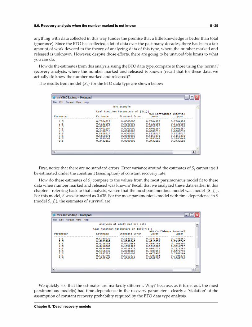
The results from model {St} for the BTO data type are shown below:
First, notice that there are no standard errors. Error variance around the estimates of Si cannot itself
be estimated under the constraint (assumption) of constant recovery rate.
How do these estimates of Si compare to the values from the most parsimonious model fit to these
data when number marked and released was known? Recall that we analyzed these data earlier in this
chapter – referring back to that analysis, we see that the most parsimonious model was model {S· ft }.
For this model, S was estimated as 0.638. For the most parsimonious model with time dependence in S
(model St ft ), the estimates of survival are
We quickly see that the estimates are markedly different. Why? Because, as it turns out, the most
parsimonious model(s) had time-dependence in the recovery parameter – clearly a ‘violation’ of the
assumption of constant recovery probability required by the BTO data type analysis.
Chapter 8. ‘Dead’ recovery models
8.7. Recovery models and GOF 8 - 26
8.7. Recovery models and GOF
First the good news – GOF testing for recovery models is possible, and quite straightforward. Now
the bad news (well, perhaps not ‘bad’ news, but something to note) – the type of GOF tests that are
available to you depends on which parameterization you use (Brownie, or Seber). If you want to use
the ‘Brownie’ parameterization, you can test goodness of fit of the data to your general model using
program ESTIMATE (Brownie et al. 1985). Program ESTIMATE can be called from within MARK
(much as you can invoke program RELEASE from within MARK). Alternatively, if you’re using the
‘Seber’ parameterization, you can use either the bootstrap or median-c approaches (but not program
ESTIMATE) for GOF testing.
But, suppose you’ve already fit your model set using the ‘Brownie’ parameterization, but instead of
using program ESTIMATE for the GOF, you’d like to estimate c using either the bootstrap or median-c
approaches. Do you need to ‘start over’, and re-construct all your ‘Brownie’ models using the equivalent
‘Seber’ parameterization? The answer (thankfully) is ‘no’. All we need to do is change the data type from
‘Brownie’ → ‘Seber’ for the general model, which we can do directly within MARK (see below).
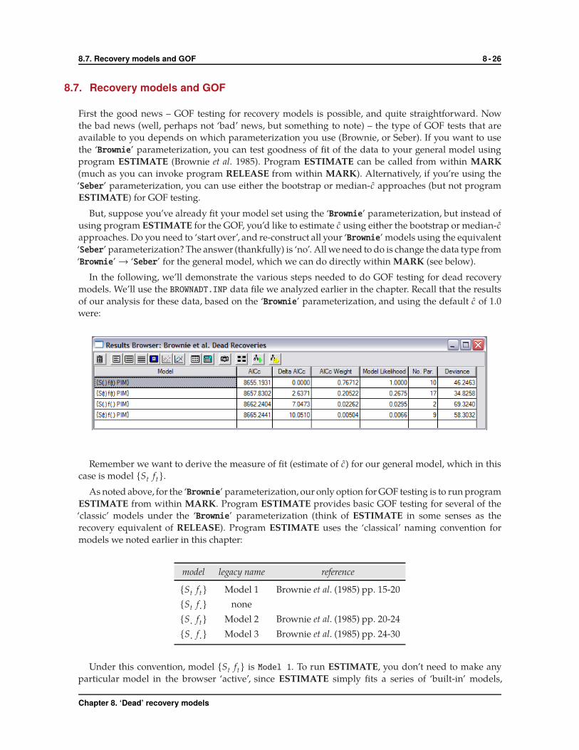
In the following, we’ll demonstrate the various steps needed to do GOF testing for dead recovery
models. We’ll use the BROWNADT.INP data file we analyzed earlier in the chapter. Recall that the results
of our analysis for these data, based on the ‘Brownie’ parameterization, and using the default c of 1.0
were:
Remember we want to derive the measure of fit (estimate of c) for our general model, which in this
case is model {St ft}.
As noted above, for the ‘Brownie’ parameterization, our only option for GOF testing is to run program
ESTIMATE from within MARK. Program ESTIMATE provides basic GOF testing for several of the
‘classic’ models under the ‘Brownie’ parameterization (think of ESTIMATE in some senses as the
recovery equivalent of RELEASE). Program ESTIMATE uses the ‘classical’ naming convention for
models we noted earlier in this chapter:
model legacy name reference
{St ft } Model 1 Brownie et al. (1985) pp. 15-20
{St f·} none
{S· ft} Model 2 Brownie et al. (1985) pp. 20-24
{S· f·} Model 3 Brownie et al. (1985) pp. 24-30
Under this convention, model {St ft} is Model 1. To run ESTIMATE, you don’t need to make any
particular model in the browser ‘active’, since ESTIMATE simply fits a series of ‘built-in’ models,
Chapter 8. ‘Dead’ recovery models

8.7. Recovery models and GOF 8 - 27
regardless of the models you have in your browser.∗ One of these models is Model 1.
To run ESTIMATE, simply pull down the ‘Test’ menu, and select ‘Program Estimate’. After a few
seconds, you’ll be dumped into the Notepad, which will present the results of the ESTIMATE analysis.
You’ll want to find the part of the output pertaining to Model 1.
After a bit of searching, you’ll find the following results for Model 1:
The observed χ2 statistics for Model 1 is 31.57, with 25 df. The P-value of observing a χ2-value
larger than 31.57 is 17.1%. If we use the model (χ2/df) as an estimate of c, then our estimate would
be (31.57/25) � 1.263.
But, what if we wanted to use either the bootstrap or median-c approaches, rather than program
ESTIMATE? Recall that both the bootstrap or median-c GOF tests are available only for the ‘Seber’
parameterization. If your models are already constructed using the ‘Seber’ parameterization, then you
simply make the general model active in the browser (by right-clicking and retrieving it), and then
proceeding as per normal.
However, if your models are constructed using the ‘Brownie’ parameteriztion, as in the present
example, then you first need to change the data type for the general model from ‘Brownie’ → ‘Seber’.
As demonstrated earlier in this chapter, this is easy to do – simply make the general model active in the
browser (by right-clicking and retrieving it), and then select ‘PIM | Change data type’. MARK will
present you with a selection of data types which are consistent with the data contained in the PIM. In
∗ This means that unless your general model is one of the ‘built-in’ models that ESTIMATE is running, you’re out of luck.
Chapter 8. ‘Dead’ recovery models

8.8. Summary 8 - 28
this case, there are only two such data types: the ‘Dead recoveries (Seber)’ (i.e., the S and r Seber
parameterization, and the ‘Dead recoveries (Brownie et al.)’ (our current data type). We want to
switch to the Seber ‘S and r’ data type, so pick the ‘Dead recoveries (Seber)’ option from the list. You
won’t see anything happen, but you’ll now be able to run a model under the ‘S and r’ parameterization.
The model we want to run is model {St rt }, which is equivalent to model {St ft}. If you want to check to
see that the underlying parameterization has now changed to ‘Seber’, look at the PIM chart (you’ll see
that the general model is now parameterized in terms of S and r – i.e., the ‘Seber’ parameterization).
Once you’ve changed the data type, go ahead and run the model, and call it model ‘S(t)r(t)’. Add
the results to the browser. You should observe that the AIC, deviance and the number of parameters
are identical to that reported for model {St ft}. Now, all you need to do is run a bootstrap or median-c
GOF test on this new model {St rt}. The mechanics for both tests were covered in detail in Chapter 5.
Based on 1,000 bootstraps, we found that approximately 21% of the bootstrapped deviances were
greater than the observed deviance for model {St rt }, indicating adequate fit. Recall from our program
ESTIMATE GOF analysis that the observed χ2 statistics for Model 1was 31.57, with 25 df. The P-value
of observing a χ2-value larger than 31.57 is 17.1%, which is comparable to the 21% value observed from
the bootstrap analysis. Further, both our bootstrapped and median-c estimates for c (1.153, and 1.110,
respectively) are consistent with the estimate of c from the ESTIMATE analysis (31.57/25 � 1.263).
Taken together, this wouldsuggest some levelof equivalence between the approachbasedon program
ESTIMATE, applied to the general model under the ‘Brownie’ parameterization, and the bootstrap and
medianc approaches, under the ‘Seber’ parameterization. Such a conclusion should be approached
cautiously. One thing the ESTIMATE output does give you is the relative contribution of each element
of the recovery matrix to the overall model χ2. This is analogous to partitioning the data into the
contingency tables that we used with program RELEASE for live encounter data. The contributions for
this data set are shown at the top of the next page. Careful examination of these tables can sometimes
help you diagnose lack of fit for recovery data.
8.8. Summary
That’s it! Recovery models are more common than you think, and not simply restricted to ‘harvested’
species. It is worth spending some time getting comfortable with the theory, and the different imple-
mentation of recovery analysis in MARK. In the next chapter, we’ll actually combine ‘dead recovery’
models with ‘live encounter’ models. As you’ll see, this ‘joint’ estimation allows you to tease apart
sources of apparent mortality in novel and potentially useful ways.
8.9. References
Anderson, D. R., Burnham, K. P., and White, G. C. (1985) Problems in estimating age-specific survival
rates from recovery data of birds ringed as young. Journal of Animal Ecology, 54, 89-98.
Brownie, C., Anderson, D. R., Burnham, K. P., and Robson, D. S. (1985) Statistical Inference from Band-
Recovery Data – A Handbook, 2nd Edition. Resource Publication No. 156. Washington, D.C.: Fish &
Wildlife Service, U.S. Department of the Interior.
Catchpole, E. A., Freeman, S. N., and Morgan, B. J. T. (1995) Modeling age variation in survival and
reporting rates for recovery models. Journal of Applied Statistics, 22, 597-609.
Lebreton, J-D., Burnham, K. P., Clobert, J., and Anderson, D. R. (1992) Modeling survival and testing
biological hypotheses using marked animals: a unified approach with case studies. Ecological
Monographs, 62, 67-118.
Chapter 8. ‘Dead’ recovery models

8.9. References 8 - 29
Seber, G. A. F. (1970) Estimating time-specific survival and reporting rates for adult birds from band
returns. Biometrika, 57, 313-318.
Chapter 8. ‘Dead’ recovery models