Chapter 9 Inference Based on Two

Samples

Motivations

• Want to study the relations between two populations, comparing their corresponding parameters

• Usually for comparative studies, trying to demonstrate certain advantages of some new treatments

• Tests used: z test for large samples or normal distribution with known variance; t test for normal distribution with small n and no sigma

• Again the population parameters considered here: mean or proportion

9.1 z Tests and CI• Assumptions:

• normal distribution with known sigma, or

• large samples (n>40, m>40)

• Assuming normal distribution with known sigma

• Sigma replaced by S in the case of large samples

• Used for (a) hypothesis testing and (b) confidence interval

Z =X − Y − (µ1 − µ2)!

!21

m + !22

n

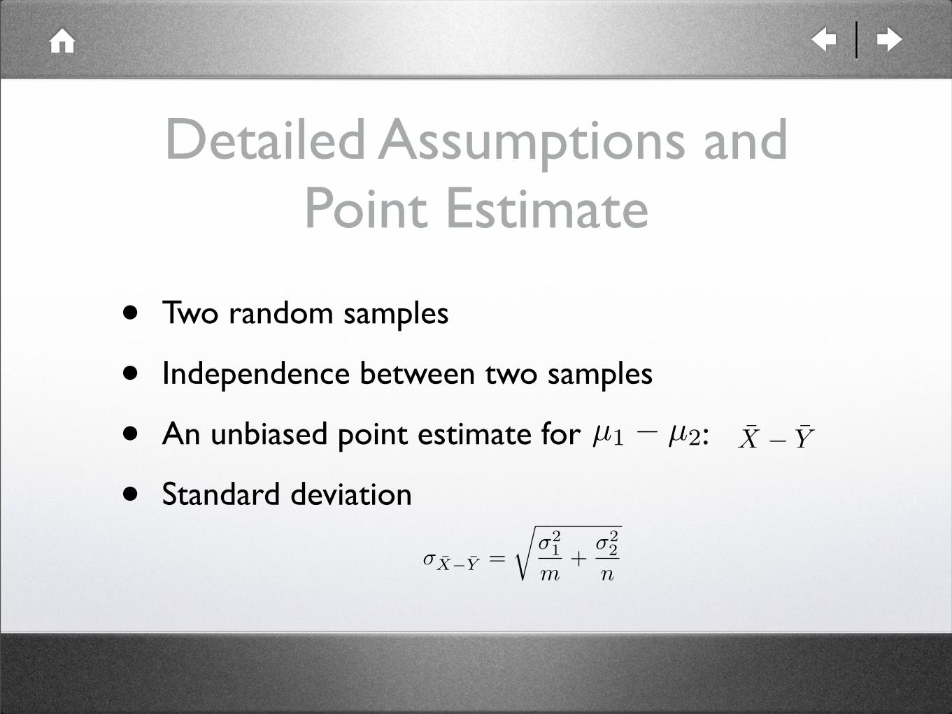
Detailed Assumptions and Point Estimate

• Two random samples

• Independence between two samples

• An unbiased point estimate for :

• Standard deviation

µ1 ! µ2 X ! Y

!X!Y =

!!2

1

m+

!22

n

Test Procedures for Hypothesis Test

• State null and alternative hypotheses

• Compute test statistic value

• Similar rejection region as in one sample procedure (replacing by )

z =x! y ! (µ1 ! µ2)!

!21

m + !22

n

µ1 ! µ2µ

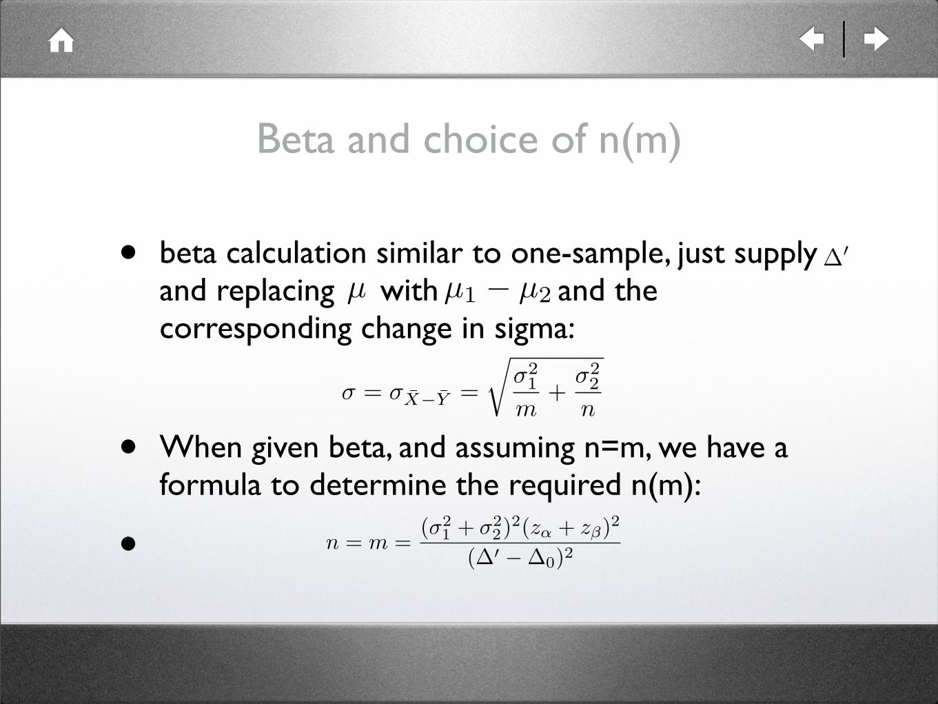
Beta and choice of n(m)

• beta calculation similar to one-sample, just supply and replacing with and the corresponding change in sigma:

• When given beta, and assuming n=m, we have a formula to determine the required n(m):

•

µ µ1 ! µ2

n = m =(!2

1 + !22)2(z! + z")2

(!! !!0)2

! = !X!Y =

!!2

1

m+

!22

n

!!

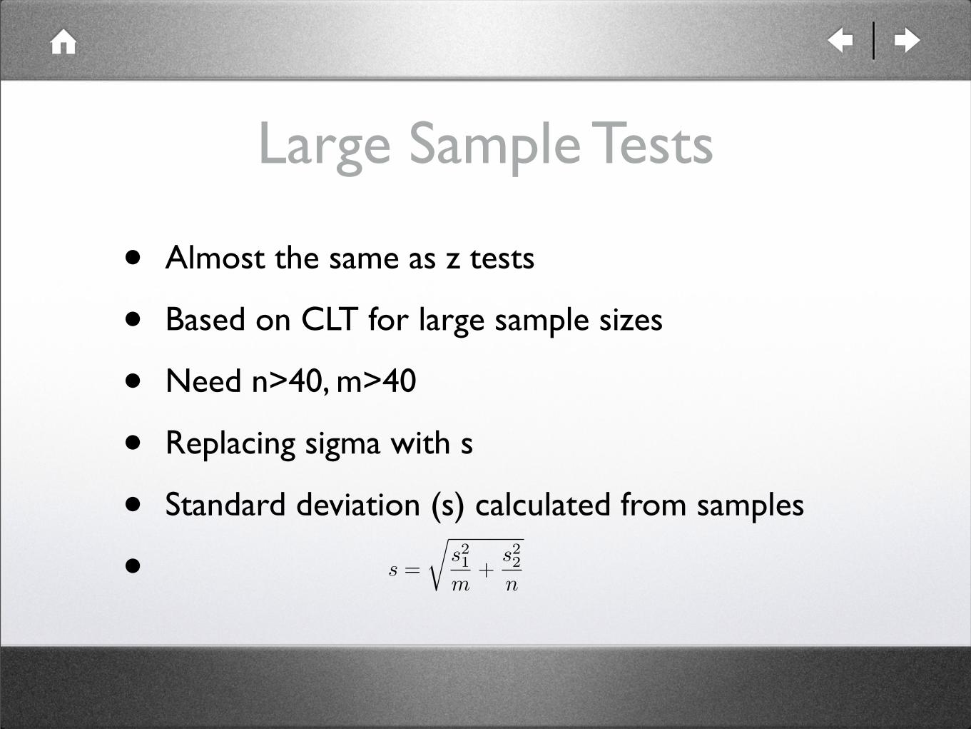
Large Sample Tests

• Almost the same as z tests

• Based on CLT for large sample sizes

• Need n>40, m>40

• Replacing sigma with s

• Standard deviation (s) calculated from samples

• s =

!s21

m+

s22

n

Confidence Interval for the Difference

• Based on the probability distribution for the z statistic

• CI with confidence level

• Similar CB: replacing with , and interval with the appropriate upper or lower bound

z! z!/2

x! y ± z!/2

!s21

m+

s22

n

9.2 Two-Sample t Test and CI

• Major loss of assumption: small sample size, sigma unknown

• Retained assumption: normal distribution

• Assumptions about random samples: similar to 9.1

• We must check the distribution before proceeding with the test

What’s Different?

• Statistic value

• Will use t critical values

• What df?

• Another notation

t =x! y !!0!

s21

m + s22

n

! =

!s21

m + s22

n

"2

(s21/m)2

m!1 + (s22/n)2

n!1

se =s!m

Pooled t Procedure• Two random samples from normal distribution

• Maybe we can assume the same variance?

• Implication: two subgroups from a large pool

• Simpler formula:

• Pros and Cons

• Very powerful when the assumption is actually correct

• Can lead to substantial errors if the assumption turns out to be wrong

z =x! y !!0!!2( 1

m + 1n )

Pooled t Procedure (continued)

• Two random samples from normal distribution

• Assuming the same variance, but not known?

• Estimated standard deviation based on two sample standard deviations:

• t test statistic: replacing with above

• What df should we use?

S2p =

m! 1m + n! 2

· S21 +

n! 1m + n! 2

· S22

! sp

m + n! 2

9.3 Analysis of Paired Data

• Two related samples, paired

• Dependence between the pairs

• Interested in relationship between the populations

• Common statistic: the mean of differences

• Two sample sizes must be the same

Difference Between Two Means

• Consider the following situations:

• Experiments involving n individuals or objects

• Each individual/object has two observations

• The observations are to be grouped according to the objects

• Obviously we shouldn’t use the two-sample test in these situations

Assumptions for the paired test

• Data consists of n independently selected pairs

• Difference for each pair

• s assumed to be normal, with variance

• Often as a consequence of normal X’s and Y’s

(X1, Y1), (X2, Y2), . . . , (Xn, Yn)

D1 = X1 ! Y1, . . . , Dn = Xn ! Yn

Di !2D

Paired t Test

• Point estimate

• Null hypothesis:

• Test statistic value

• Alternative hypothesis Rejection region

• P-value can also be calculated as earlier t tests

µD = E(X ! Y ) = µ1 ! µ2

H0 : µd = !0

t =d!!0

sD/"

n

Ha : µD > !0 t ! t!,n!1

Ha : µD < !0 t " #t!,n!1

Ha : µD $= !0 |t| ! t!/2,n!1

Confidence Interval

• Use

• The paired t CI for is

• is the sample standard deviation of D’s

• Similar for confidence bounds (replacing with )

T =D ! µD

SD/"

n

µD!

d! t!/2,n!1 · sD"n

, d + t!/2,n!1 · sD"n

"

t!/2,n!1

t!,n!1

sD

Paired vs Two-Sample

• When to use paired or two-sample?

• Check correlation to see if it is small

• If small, two-sample is appropriate

• If not small, need to make adjustment according to the sign of correlation

• Preference regarding df, balanced with increased precision in pairing

9.4 Inferences Concerning a Difference Between Population

Proportions

It’s all about proportions

• Two populations: populations #1 and #2, with proportions

• Need to estimate

• Obvious estimator

• Distribution of the estimator? normal (large m, n) vs binomial

• Proposition:

•

p1, p2

p1 ! p2

p1 ! p2 =X

m! Y

n

X ! Bin(m, p1), Y ! Bin(n, p2)E (p1 " p2) = p1 " p2

V (p1 " p2) =p1q1

m+

p2q2

n

Large-Sample Test Procedure

• Normal distribution - another application of CLT

• Use z-statistic

• Standard deviation of the estimate:

• Test of hypothesis:

• if the null suggests

• use

!p1q1

m+

p2q2

n

p1 ! p2 = 0!

pq

"1m

+1n

#p =

X + Y

m + n, q = 1! p

Large-Sample CI for Proportion Difference

• Estimated standard deviation of the difference

• Confidence interval at level

• p1 ! p2 ± z!/2

!p1q1

m+

p2q2

n

!p1q1

m+

p2q2

n!

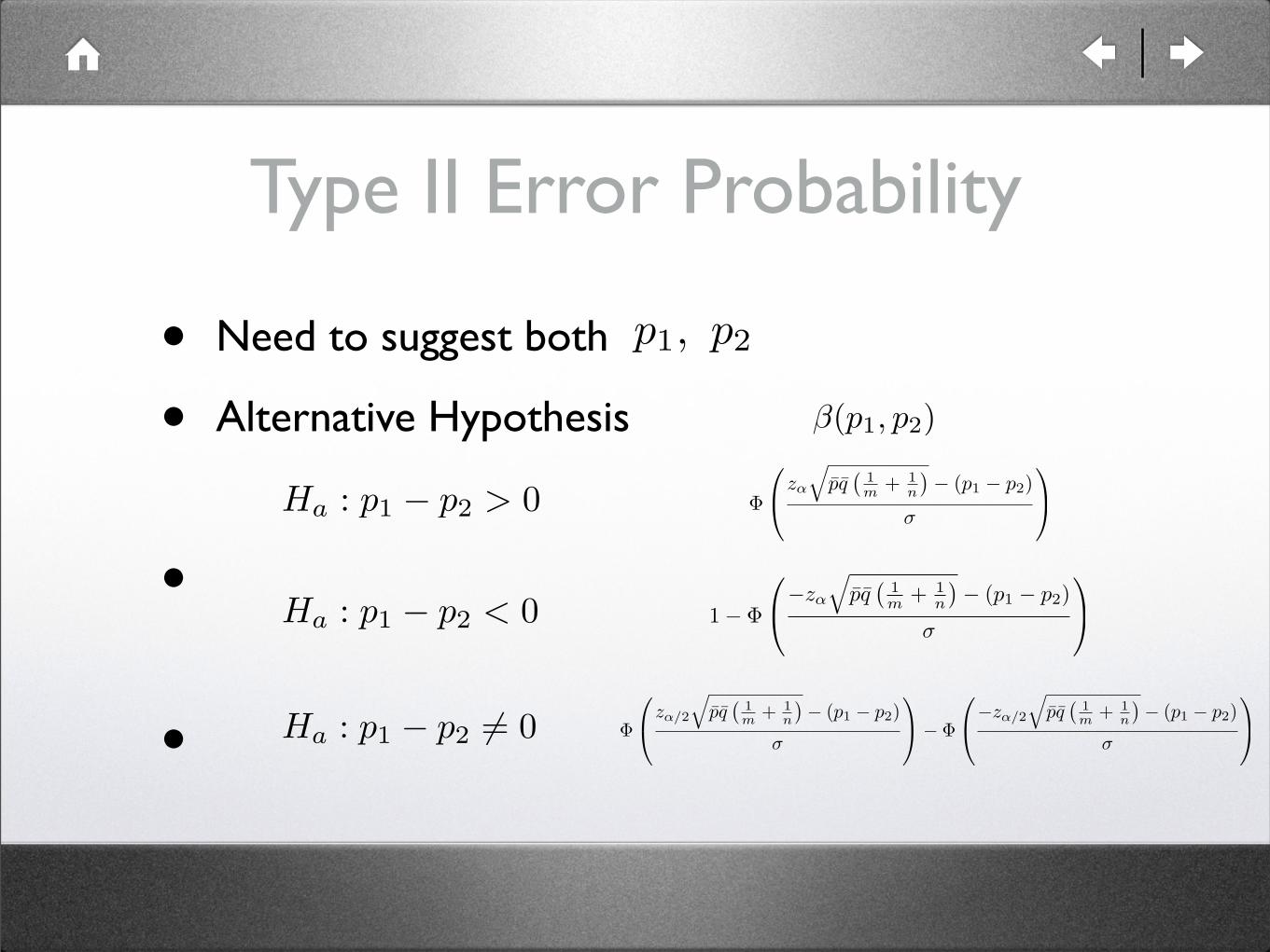
Type II Error Probability

• Need to suggest both

• Alternative Hypothesis

•

•

p1, p2

!(p1, p2)

Ha : p1 ! p2 > 0

Ha : p1 ! p2 < 0

Ha : p1 ! p2 "= 0

!

!

"z!

#pq

$1m + 1

n

%! (p1 ! p2)

!

&

'

1! !

!

"!z!

#pq

$1m + 1

n

%! (p1 ! p2)

!

&

'

!

!

"z!/2

#pq

$1m + 1

n

%! (p1 ! p2)

!

&

'! !

!

"!z!/2

#pq

$1m + 1

n

%! (p1 ! p2)

!

&

'

p =mp1 + np2

m + n, q =

mq1 + nq2

m + n

! =!

p1q1

m+

p2q2

n

Type II Error Probability• parameters used in above formulas:

9.5 Inferences Concerning Two Population Variances

Comparing Variances• Consider the ratio instead of difference

• A new distribution: F distribution

• Referring to the ratio of two independent chi-squared rv’s with respective df’s

• Two parameters (df’s)

• Critical values:

F =X1/!1

X2/!2

F1!!,"1,"2 =1

F!,"1,"2

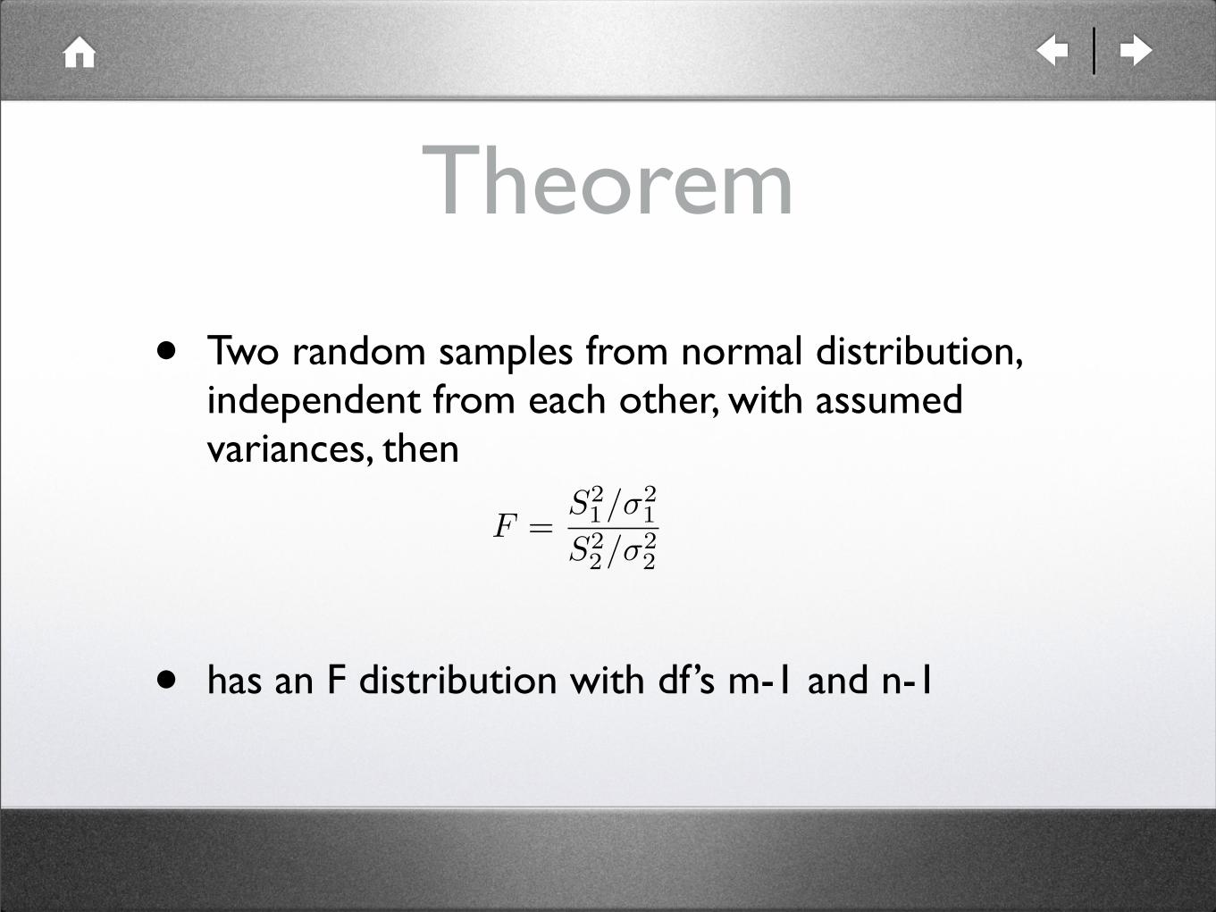
Theorem

• Two random samples from normal distribution, independent from each other, with assumed variances, then

• has an F distribution with df’s m-1 and n-1

F =S2

1/!21

S22/!2

2

F Test

• Null hypothesis:

• Test statistic value

• Alternative hypothesis Rejection region

•

H0 : !21 = !2

2

f = s21/s2

2

Ha : !21 > !2

2

Ha : !21 < !2

2

Ha : !21 != !2

2

f ! F!,m!1,n!1

f ! F1!!,m!1,n!1

f ! F!/2,m!1,n!1 or f " F1!!/2,m!1,n!1