399

Chapter 9 MEMORY MANAGEMENT

In Chapter 6, we showed how the CPU can be shared by a set of processes. As a result of CPU scheduling, we can improve both the utilization of the CPU and the speed of the computer's response to its users. To realize this increase in performance, however, we must keep several processes in memory; that is, we must share memory.

In this chapter, we discuss various ways to manage memory. The memory-management algorithms vary from a primitive bare-machine approach to paging and segmentation strategies. Each approach has its own advantages and disadvantages. Selection of a memory-management method for a specific system depends on many factors, especially on the hardware design of the system. As we shall see, many algorithms require hardware support, although recent designs have closely integrated the hardware and operating system.

9.1 Background

As we saw in Chapter 1, memory is central to the operation of a modern computer system. Memory consists of a large array of words or bytes, each with its own address. The CPU fetches instructions from memory according to the value of the program counter. These instructions may cause additional loading from and storing to specific memory addresses.

A typical instruction-execution cycle, for example, first fetches an instruction from memory. The instruction is then decoded and may cause operands to be fetched from memory. After the instruction has been executed on the operands, results may be stored back in memory. The memory unit sees only a stream of memory addresses; it

400

does not know how they are generated (by the instruction counter, indexing, indirection, literal addresses, and so on) or what they are for (instructions or data). Accordingly, we can ignore how a program generates a memory address. We are interested only in the sequence of memory addresses generated by the running program.

9.1.1 Address Binding

Usually, a program resides on a disk as a binary executable file. To be executed, the program must be brought into memory and placed within a process. Depending on the memory management in use, the process may be moved between disk and memory during its execution. The processes on the disk that are waiting to be brought into memory for execution form the input queue.

The normal procedure is to select one of the processes in the input queue and to load that process into memory. As the process is executed, it accesses instructions and data from memory. Eventually, the process terminates, and its memory space is declared available.

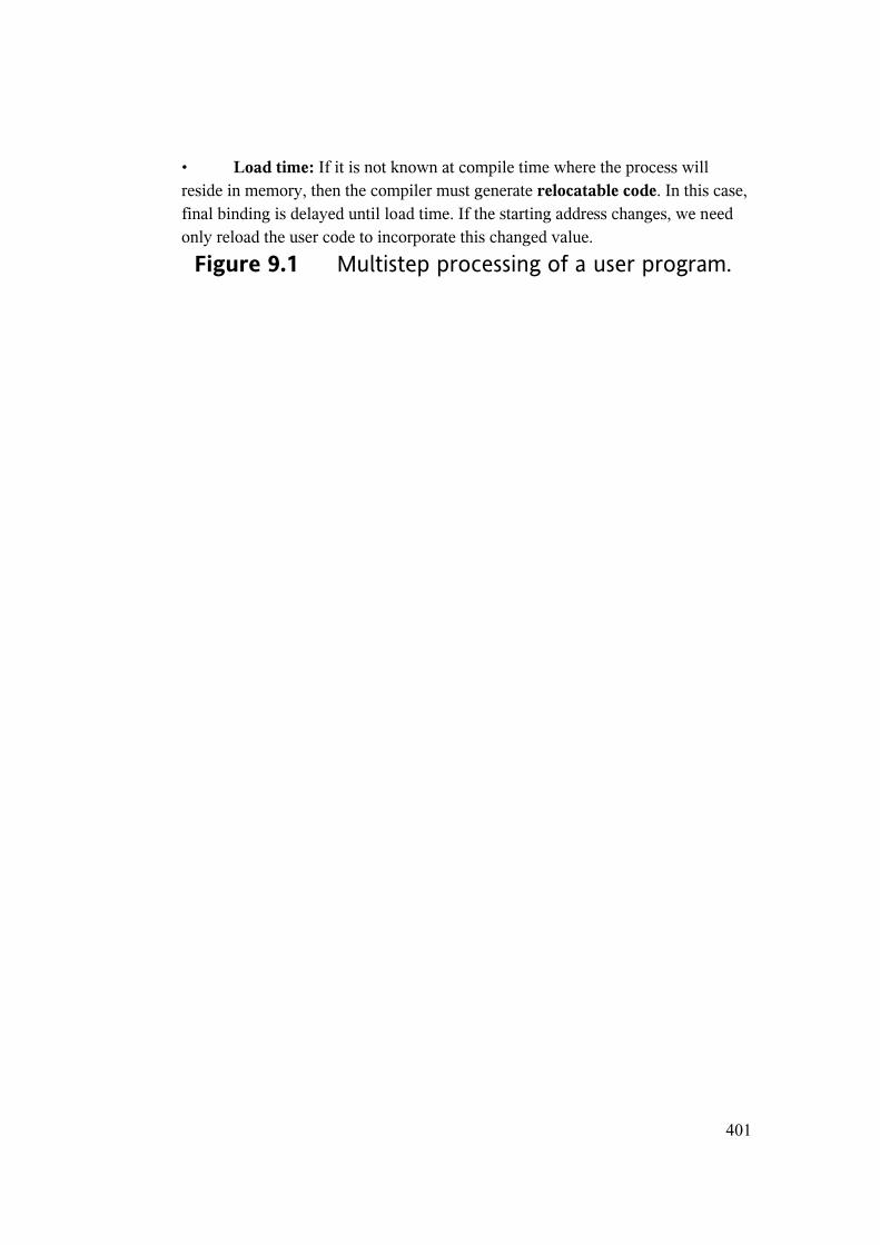
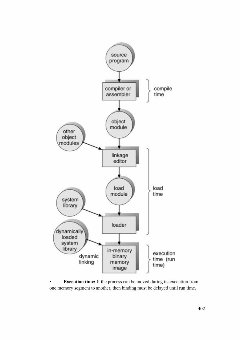
Most systems allow a user process to reside in any part of the physical memory. Thus, although the address space of the computer starts at 00000, the first address of the user process need not be 00000. This approach affects the addresses that the user program can use. In most cases, a user program will go through several steps—some of which may be optional—before being executed (Figure 9.1). Addresses may be represented in different ways during these steps. Addresses in the source program are generally symbolic (such as count). A compiler will typically bindthese symbolic addresses to relocatable addresses (such as "14 bytes from the beginning of this module"). The linkage editor or loader will in turn bind the relocatable addresses to absolute addresses (such as 74014). Each binding is a mapping from one address space to another.

Classically, the binding of instructions and data to memory addresses can be done at any step along the way:

• Compile time: If you know at compile time where the process will reside in memory, then absolute code can be generated. For example, if you know that a user process will reside starting at location R, then the generated compiler code will start at that location and extend up from there. If, at some later time, the starting location changes, then it will be necessary to recompile this code. The MS-DOS .COM-format programs are bound at compile time.

401

• Load time: If it is not known at compile time where the process will reside in memory, then the compiler must generate relocatable code. In this case, final binding is delayed until load time. If the starting address changes, we need only reload the user code to incorporate this changed value.

Figure 9.1 Multistep processing of a user program.

402

• Execution time: If the process can be moved during its execution from one memory segment to another, then binding must be delayed until run time.

403

Special hardware must be available for this scheme to work, as will be discussed in Section 9.1.2. Most general-purpose operating systems use this method.

A major portion of this chapter is devoted to showing how these various bindings can be implemented effectively in a computer system and to discussing appropriate hardware support.

9.1.2 Logical- versus Physical-Address Space

An address generated by the CPU is commonly referred to as a logical address, whereas an address seen by the memory unit—that is, the one loaded into the memory-address register of the memory—is commonly referred to as a physical address.

The compile-time and load-time address-binding methods generate identical logical and physical addresses. However, the execution-time address-binding scheme results in differing logical and physical addresses. In this case, we usually refer to the logical address as a virtual address. We use logical address and virtual addressinterchangeably in this text. The set of all logical addresses generated by a program is a logical-address space; the set of all physical addresses corresponding to these logical addresses is a physical-address space. Thus, in the execution-time address-binding scheme, the logical- and physical-address spaces differ.

The run-time mapping from virtual to physical addresses is done by a hardware device called the memory-management unit (MMU). We can choose from many different methods to accomplish such mapping, as we discuss in Sections 9.1through 9.1. For the time being, we illustrate this mapping with a simple MMU

scheme, which is a generalization of the base-register scheme described in Section 2.5.3.

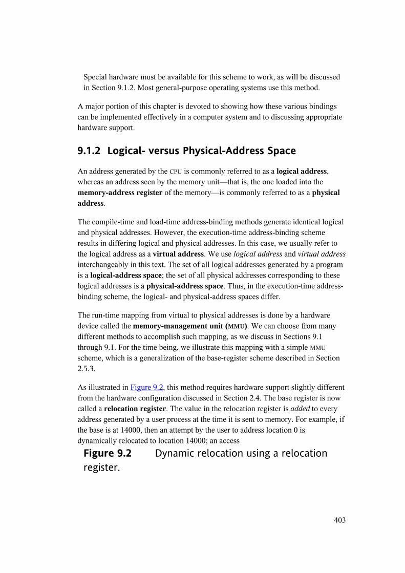
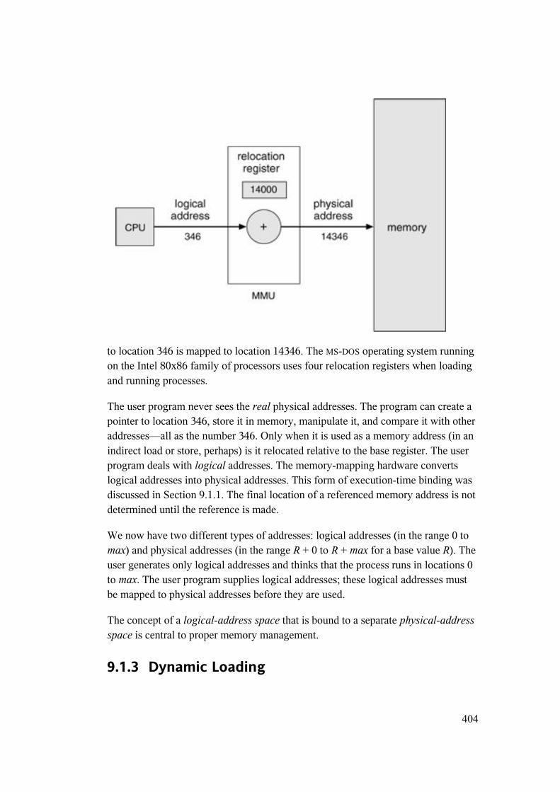
As illustrated in Figure 9.2, this method requires hardware support slightly different from the hardware configuration discussed in Section 2.4. The base register is now called a relocation register. The value in the relocation register is added to every address generated by a user process at the time it is sent to memory. For example, if the base is at 14000, then an attempt by the user to address location 0 is dynamically relocated to location 14000; an access

Figure 9.2 Dynamic relocation using a relocation register.

404

to location 346 is mapped to location 14346. The MS-DOS operating system running on the Intel 80x86 family of processors uses four relocation registers when loading and running processes.

The user program never sees the real physical addresses. The program can create a pointer to location 346, store it in memory, manipulate it, and compare it with other addresses—all as the number 346. Only when it is used as a memory address (in an indirect load or store, perhaps) is it relocated relative to the base register. The user program deals with logical addresses. The memory-mapping hardware converts logical addresses into physical addresses. This form of execution-time binding was discussed in Section 9.1.1. The final location of a referenced memory address is not determined until the reference is made.

We now have two different types of addresses: logical addresses (in the range 0 to max) and physical addresses (in the range R + 0 to R + max for a base value R). The user generates only logical addresses and thinks that the process runs in locations 0to max. The user program supplies logical addresses; these logical addresses must be mapped to physical addresses before they are used.

The concept of a logical-address space that is bound to a separate physical-address space is central to proper memory management.

9.1.3 Dynamic Loading

405

In our discussion so far, the entire program and all data of a process must be in physical memory for the process to execute. The size of a process is thus limited to the size of physical memory. To obtain better memory-space utilization, we can use dynamic loading. With dynamic loading, a routine is not loaded until it is called. All routines are kept on disk in a relocatable load format. The main program is loaded into memory and is executed. When a routine needs to call another routine, the calling routine first checks to see whether the other routine has been loaded. If not, the relocatable linking loader is called to load the desired routine into memory and to update the program's address tables to reflect this change. Then control is passed to the newly loaded routine.

The advantage of dynamic loading is that an unused routine is never loaded. This method is particularly useful when large amounts of code are needed to handle infrequently occurring cases, such as error routines. In this case, although the total program size may be large, the portion that is used (and hence loaded) may be much smaller.

Dynamic loading does not require special support from the operating system. It is the responsibility of the users to design their programs to take advantage of such a method. Operating systems may help the programmer, however, by providing library routines to implement dynamic loading.

9.1.4 Dynamic Linking and Shared Libraries

Figure 9.1 also shows dynamically linked libraries. Some operating systems support only static linking, in which system language libraries are treated like any other object module and are combined by the loader into the binary program image. The concept of dynamic linking is similar to that of dynamic loading. Here, though, linking, rather than loading, is postponed until execution time. This feature is usually used with system libraries, such as language subroutine libraries. Without this facility, each program on a system must have a copy of its language library (or at least the routines referenced by the program) included in the executable image. This requirement wastes both disk space and main memory.

With dynamic linking, a stub is included in the image for each library-routine reference. The stub is a small piece of code that indicates how to locate the appropriate memory-resident library routine or how to load the library if the routine is not already present. When the stub is executed, it checks to see whether the needed routine is already in memory. If not, the program loads the routine into memory. Either way, the stub replaces itself with the address of the routine and

406

executes the routine. Thus, the next time that particular code segment is reached, the library routine is executed directly, incurring no cost for dynamic linking. Under this scheme, all processes that use a language library execute only one copy of the library code.

This feature can be extended to library updates (such as bug fixes). A library may be replaced by a new version, and all programs that reference the library will automatically use the new version. Without dynamic linking, all such programs would need to be relinked to gain access to the new library. So that programs will not accidentally execute new, incompatible versions of libraries, version information is included in both the program and the library. More than one version of a library may be loaded into memory, and each program uses its version information to decide which copy of the library to use. Minor changes retain the same version number, whereas major changes increment the version number. Thus, only programs that are compiled with the new library version are affected by the incompatible changes incorporated in it. Other programs linked before the new library was installed will continue using the older library. This system is also known as shared libraries.

Unlike dynamic loading, dynamic linking generally requires help from the operating system. If the processes in memory are protected from one another (Section 9.3), then the operating system is the only entity that can check to see whether the needed routine is in another process's memory space or that can allow multiple processes to access the same memory addresses. We elaborate on this concept when we discuss paging in Section 9.4.5.

9.1.5 Overlays

To enable a process to be larger than the amount of memory allocated to it, we can use overlays. The idea of overlays is to keep in memory only those instructions and data that are needed at any given time. When other instructions are needed, they are loaded into space occupied previously by instructions that are no longer needed.

As an example, consider a two-pass assembler. During pass 1, it constructs a symbol table; then, during pass 2, it generates machine-language code. We may be able to partition such an assembler into pass 1 code, pass 2 code, the symbol table, and common support routines used by both pass 1 and pass 2. Assume that the sizes of these components are as follows:

Pass 1

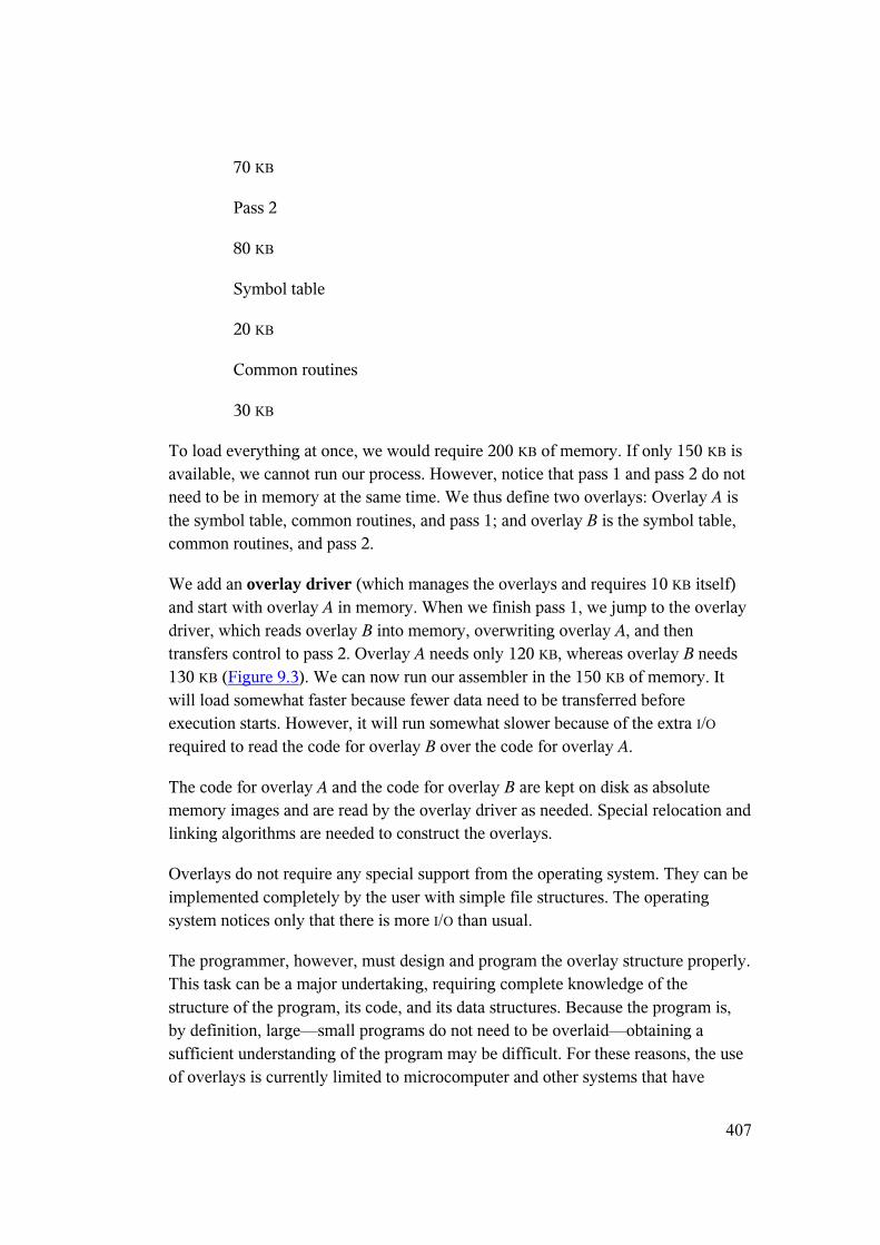
407

70 KB

Pass 2

80 KB

Symbol table

20 KB

Common routines

30 KB

To load everything at once, we would require 200 KB of memory. If only 150 KB is available, we cannot run our process. However, notice that pass 1 and pass 2 do not need to be in memory at the same time. We thus define two overlays: Overlay A is the symbol table, common routines, and pass 1; and overlay B is the symbol table, common routines, and pass 2.

We add an overlay driver (which manages the overlays and requires 10 KB itself) and start with overlay A in memory. When we finish pass 1, we jump to the overlay driver, which reads overlay B into memory, overwriting overlay A, and then transfers control to pass 2. Overlay A needs only 120 KB, whereas overlay B needs 130 KB (Figure 9.3). We can now run our assembler in the 150 KB of memory. It will load somewhat faster because fewer data need to be transferred before execution starts. However, it will run somewhat slower because of the extra I/Orequired to read the code for overlay B over the code for overlay A.

The code for overlay A and the code for overlay B are kept on disk as absolute memory images and are read by the overlay driver as needed. Special relocation and linking algorithms are needed to construct the overlays.

Overlays do not require any special support from the operating system. They can be implemented completely by the user with simple file structures. The operating system notices only that there is more I/O than usual.

The programmer, however, must design and program the overlay structure properly. This task can be a major undertaking, requiring complete knowledge of the structure of the program, its code, and its data structures. Because the program is, by definition, large—small programs do not need to be overlaid—obtaining a sufficient understanding of the program may be difficult. For these reasons, the use of overlays is currently limited to microcomputer and other systems that have

408

limited amounts of physical memory and that lack hardware support for more advanced techniques. Some microcomputer compilers provide the programmer with support for overlays to make the task easier. Automatic techniques to run large programs in limited amounts of physical memory are certainly preferable.

Figure 9.3 Overlays for a two-pass assembler.

9.2 Swapping

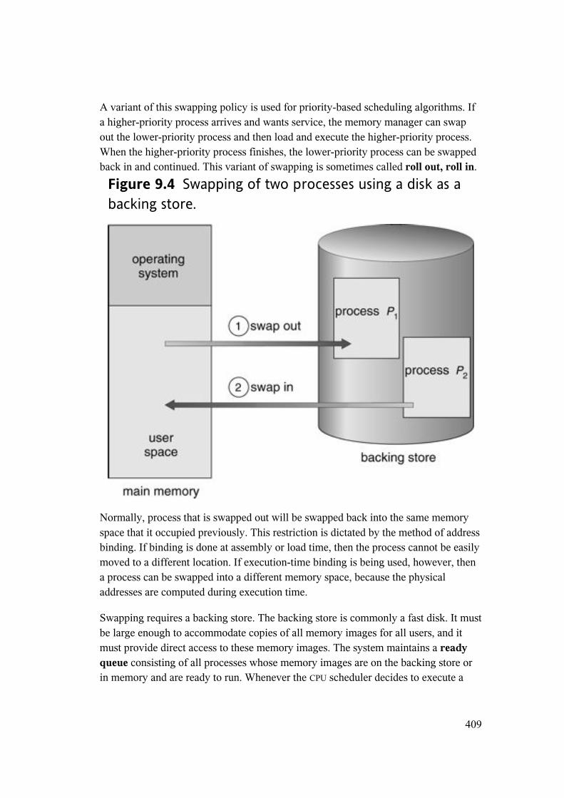
A process must be in memory to be executed. A process, however, can be swappedtemporarily out of memory to a backing store and then brought back into memory for continued execution. For example, assume a multiprogramming environment with a round-robin CPU-scheduling algorithm. When a quantum expires, the memory manager will start to swap out the process that just finished and to swap another process into the memory space that has been freed (Figure 9.4). In the meantime, the CPU scheduler will allocate a time slice to some other process in memory. When each process finishes its quantum, it will be swapped with another process. Ideally, the memory manager can swap processes fast enough that some processes will be in memory, ready to execute, when the CPU scheduler wants to reschedule the CPU. In addition, the quantum must be sufficiently large that reasonable amounts of computing are done between swaps.

409

A variant of this swapping policy is used for priority-based scheduling algorithms. If a higher-priority process arrives and wants service, the memory manager can swap out the lower-priority process and then load and execute the higher-priority process. When the higher-priority process finishes, the lower-priority process can be swapped back in and continued. This variant of swapping is sometimes called roll out, roll in.

Figure 9.4 Swapping of two processes using a disk as a backing store.

Normally, process that is swapped out will be swapped back into the same memory space that it occupied previously. This restriction is dictated by the method of address binding. If binding is done at assembly or load time, then the process cannot be easily moved to a different location. If execution-time binding is being used, however, then a process can be swapped into a different memory space, because the physical addresses are computed during execution time.

Swapping requires a backing store. The backing store is commonly a fast disk. It must be large enough to accommodate copies of all memory images for all users, and it must provide direct access to these memory images. The system maintains a ready queue consisting of all processes whose memory images are on the backing store or in memory and are ready to run. Whenever the CPU scheduler decides to execute a

410

process, it calls the dispatcher. The dispatcher checks to see whether the next process in the queue is in memory. If it is not, and if there is no free memory region, the dispatcher swaps out a process currently in memory and swaps in the desired process. It then reloads registers and transfers control to the selected process.

The context-switch time in such a swapping system is fairly high. To get an idea of the context-switch time, let us assume that the user process is of size 1 MB and the backing store is a standard hard disk with a transfer rate of 5 MB per second. The actual transfer of the 1-MB process to or from main memory takes

1000 KB/5000 KB per second

=

1/5 second

=

200 milliseconds.

Assuming that no seeks are necessary and an average latency of 8 milliseconds, the swap time is 208 milliseconds. Since we must both swap out and swap in, the total swap time is then about 416 milliseconds.

For efficient CPU utilization, we want the execution time for each process to be long relative to the swap time. Thus, in a round-robin CPU-scheduling algorithm, for example, the time quantum should be substantially larger than 0.416 seconds.

Notice that the major part of the swap time is transfer time. The total transfer time is directly proportional to the amount of memory swapped. If we have a computer system with 128 MB of main memory and a resident operating system taking 5 MB, the maximum size of the user process is 123 MB. However, many user processes may be much smaller than this size—say, 1 MB. A 1-MB process could be swapped out in 208 milliseconds, compared with the 24.6 seconds required for swapping 123 MB. Clearly, it would be useful to know exactly how much memory a user process is using, not simply how much it might be using. Then, we would need to swap only what is actually used, reducing swap time. For this method to be effective, the user must keep the system informed of any changes in memory requirements. Thus, a process with dynamic memory requirements will need to issue system calls (request memoryand release memory) to inform the operating system of its changing memory needs.

411

Swapping is constrained by other factors as well. If we want to swap a process, we must be sure that it is completely idle. Of particular concern is any pending I/O. A process may be waiting for an I/O operation when we want to swap that process to free up memory. However, if the I/O is asynchronously accessing the user memory for I/O buffers, then the process cannot be swapped. Assume that the I/O operation is queued because the device is busy. If we were to swap out process P1 and swap in process P2, the I/O operation might then attempt to use memory that now belongs to process P2. There are two main solutions to this problem: Never swap a process with pending I/O, or execute I/O operations only into operating-system buffers. Transfers between operating-system buffers and process memory then occur only when the process is swapped in.

The assumption, mentioned earlier, that swapping requires few, if any, head seeks needs further explanation. We postpone discussing this issue until Chapter 14, where secondary-storage structure is covered. Generally, swap space is allocated as a chunk of disk, separate from the file system, so that its use is as fast as possible.

Currently, standard swapping is used in few systems. It requires too much swapping time and provides too little execution time to be a reasonable memory-management solution. Modified versions of swapping, however, are found on many systems.

A modification of swapping is used in many versions of UNIX. Swapping is normally disabled but will start if many processes are running and are using a threshold amount of memory. Swapping is again halted when the load on the system is reduced. Memory management in UNIX is described fully in Section A.6.

Early PCs—which lacked the sophistication to implement more advanced memory-management methods—ran multiple large processes by using a modified version of swapping. A prime example is the Microsoft Windows 3.1 operating system, which supports concurrent execution of processes in memory. If a new process is loaded and there is insufficient main memory, an old process is swapped to disk. This operating system, however, does not provide full swapping, because the user, rather than the scheduler, decides when it is time to preempt one process for another. Any swapped-out process remains swapped out (and not executing) until the user selects that process to run. Subsequent versions of Microsoft operating systems take advantage of advanced MMU features now found in PCs. We will explore such features in Section 9.4 and in Chapter 10, where we cover virtual memory.

9.3 Contiguous-Memory Allocation

412

The main memory must accommodate both the operating system and the various user processes. We therefore need to allocate the parts of the main memory in the most efficient way possible. This section explains one common method, contiguous memory allocation.

The memory is usually divided into two partitions: one for the resident operating system and one for the user processes. We can place the operating system in either low memory or high memory. The major factor affecting this decision is the location of the interrupt vector. Since the interrupt vector is often in low memory, programmers usually place the operating system in low memory as well. Thus, in this text, we discuss only the situation where the operating system resides in low memory. The development of the other situation is similar.

We usually want several user processes to reside in memory at the same time. We therefore need to consider how to allocate available memory to the processes that are in the input queue waiting to be brought into memory. In this contiguous-memoryallocation, each process is contained in a single contiguous section of memory.

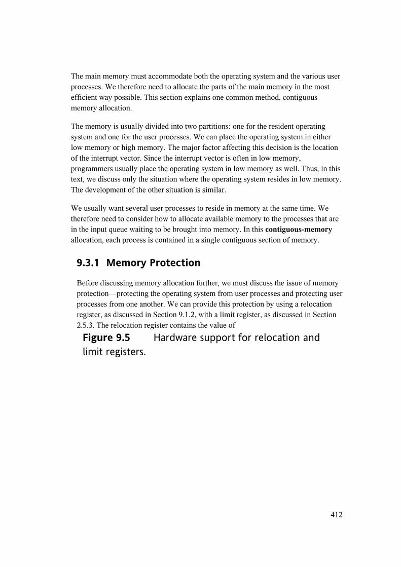
9.3.1 Memory Protection

Before discussing memory allocation further, we must discuss the issue of memory protection—protecting the operating system from user processes and protecting user processes from one another. We can provide this protection by using a relocation register, as discussed in Section 9.1.2, with a limit register, as discussed in Section 2.5.3. The relocation register contains the value of

Figure 9.5 Hardware support for relocation and limit registers.

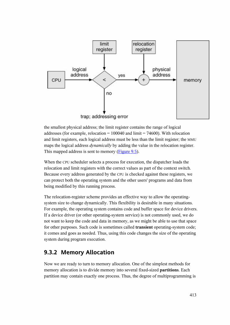
413

the smallest physical address; the limit register contains the range of logical addresses (for example, relocation = 100040 and limit = 74600). With relocation and limit registers, each logical address must be less than the limit register; the MMU

maps the logical address dynamically by adding the value in the relocation register. This mapped address is sent to memory (Figure 9.5).

When the CPU scheduler selects a process for execution, the dispatcher loads the relocation and limit registers with the correct values as part of the context switch. Because every address generated by the CPU is checked against these registers, we can protect both the operating system and the other users' programs and data from being modified by this running process.

The relocation-register scheme provides an effective way to allow the operating-system size to change dynamically. This flexibility is desirable in many situations. For example, the operating system contains code and buffer space for device drivers. If a device driver (or other operating-system service) is not commonly used, we do not want to keep the code and data in memory, as we might be able to use that space for other purposes. Such code is sometimes called transient operating-system code; it comes and goes as needed. Thus, using this code changes the size of the operating system during program execution.

9.3.2 Memory Allocation

Now we are ready to turn to memory allocation. One of the simplest methods for memory allocation is to divide memory into several fixed-sized partitions. Each partition may contain exactly one process. Thus, the degree of multiprogramming is

414

bound by the number of partitions. In this multiple-partition method, when a partition is free, a process is selected from the input queue and is loaded into the free partition. When the process terminates, the partition becomes available for another process. This method was originally used by the IBM OS/360 operating system (called MFT); it is no longer in use. The method described next is a generalization of the fixed-partition scheme (called MVT); it is used primarily in a batch environment. Many of the ideas presented here are also applicable to a time-sharing environment in which pure segmentation is used for memory management (Section 9.5).

In the fixed-partition scheme, the operating system keeps a table indicating which parts of memory are available and which are occupied. Initially, all memory is available for user processes and is considered as one large block of available memory, a hole. When a process arrives and needs memory, we search for a hole large enough for this process. If we find one, we allocate only as much memory as is needed, keeping the rest available to satisfy future requests.

As processes enter the system, they are put into an input queue. The operating system takes into account the memory requirements of each process and the amount of available memory space in determining which processes are allocated memory. When a process is allocated space, it is loaded into memory, and it can then compete for the CPU. When a process terminates, it releases its memory, which the operating system may then fill with another process from the input queue.

At any given time, we have a list of available block sizes and the input queue. The operating system can order the input queue according to a scheduling algorithm. Memory is allocated to processes until, finally, the memory requirements of the next process cannot be satisfied—that is, no available block of memory (or hole) is large enough to hold that process. The operating system can then wait until a large enough block is available, or it can skip down the input queue to see whether the smaller memory requirements of some other process can be met.

In general, at any given time we have a set of holes of various sizes scattered throughout memory. When a process arrives and needs memory, the system searches the set for a hole that is large enough for this process. If the hole is too large, it is split into two parts. One part is allocated to the arriving process; the other is returned to the set of holes. When a process terminates, it releases its block of memory, which is then placed back in the set of holes. If the new hole is adjacent to other holes, these adjacent holes are merged to form one larger hole. At this point, the system may need to check whether there are processes waiting for memory and

415

whether this newly freed and recombined memory could satisfy the demands of any of these waiting processes.

This procedure is a particular instance of the general dynamic storage-allocation problem, which concerns how to satisfy a request of size n from a list of free holes. There are many solutions to this problem. The first-fit, best-fit, and worst-fitstrategies are the ones most commonly used to select a free hole from the set of available holes.

• First fit: Allocate the first hole that is big enough. Searching can start either at the beginning of the set of holes or where the previous first-fit search ended. We can stop searching as soon as we find a free hole that is large enough.

• Best fit: Allocate the smallest hole that is big enough. We must search the entire list, unless the list is ordered by size. This strategy produces the smallest leftover hole.

• Worst fit: Allocate the largest hole. Again, we must search the entire list, unless it is sorted by size. This strategy produces the largest leftover hole, which may be more useful than the smaller leftover hole from a best-fit approach.

Simulations have shown that both first fit and best fit are better than worst fit in terms of decreasing time and storage utilization. Neither first fit nor best fit is clearly better than the other in terms of storage utilization, but first fit is generally faster.

9.3.3 Fragmentation

Both the first-fit and the best-fit strategies for memory allocation suffer from external fragmentation. As processes are loaded and removed from memory, the free memory space is broken into little pieces. External fragmentation exists when there is enough total memory space to satisfy a request, but the available spaces are not contiguous; storage is fragmented into a large number of small holes. This fragmentation problem can be severe. In the worst case, we could have a block of free (or wasted) memory between every two processes. If all these small pieces of memory were in one big free block instead, we might be able to run several more processes.

Whether we are using the first-fit or best-fit strategy can affect the amount of fragmentation. (First fit is better for some systems, whereas best fit is better for others.) Another factor is which end of a free block is allocated. (Which is the

416

leftover piece—the one on the top, or the one on the bottom?) No matter which algorithm is used, external fragmentation will be a problem.

Depending on the total amount of memory storage and the average process size, external fragmentation may be a minor or a major problem. Statistical analysis of first fit, for instance, reveals that, even with some optimization, given N allocated blocks, another 0.5N blocks will be lost to fragmentation. That is, one-third ofmemory may be unusable! This property is known as the 50-percent rule.

Memory fragmentation can be internal as well as external. Consider a multiple-partition allocation scheme with a hole of 18,464 bytes. Suppose that the next process requests 18,462 bytes. If we allocate exactly the requested block, we are left with a hole of 2 bytes. The overhead to keep track of this hole will be substantially larger than the hole itself. The general approach to avoiding this problem is to break the physical memory into fixed-sized blocks and allocate memory in units based on block size. With this approach, the memory allocated to a process may be slightly larger than the requested memory. The difference between these two numbers is internal fragmentation—memory that is internal to a partition but is not being used.

One solution to the problem of external fragmentation is compaction. The goal is to shuffle the memory contents so as to place all free memory together in one large block. Compaction is not always possible, however. If relocation is static and is done at assembly or load time, compaction cannot be done; compaction is possible only if relocation is dynamic and is done at execution time. If addresses are relocated dynamically, relocation requires only moving the program and data and then changing the base register to reflect the new base address. When compaction is possible, we must determine its cost. The simplest compaction algorithm is to move all processes toward one end of memory; all holes move in the other direction, producing one large hole of available memory. This scheme can be expensive.

Another possible solution to the external-fragmentation problem is to permit the logical-address space of a process to be noncontiguous, thus allowing a process to be allocated physical memory wherever the latter is available. Two complementary techniques achieve this solution: paging (Section 9.4) and segmentation (Section 9.5). These techniques can also be combined (Section 9.6).

9.4 Paging

Paging is a memory-management scheme that permits the physical-address space of a process to be noncontiguous. Paging avoids the considerable problem of fitting

417

memory chunks of varying sizes onto the backing store; most memory-management schemes used before the introduction of paging suffered from this problem. The problem arises because, when some code fragments or data residing in main memory need to be swapped out, space must be found on the backing store. The backing store also has the fragmentation problems discussed in connection with main memory, except that access is much slower, so compaction is impossible. Because of its advantages over earlier methods, paging in its various forms is commonly used in most operating systems.

Traditionally, support for paging has been handled by hardware. However, recent designs have implemented paging by closely integrating the hardware and operating system, especially on 64-bit microprocessors.

9.4.1 Basic Method

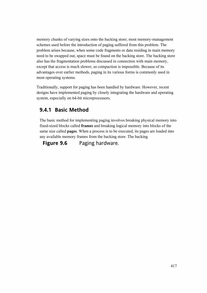
The basic method for implementing paging involves breaking physical memory into fixed-sized blocks called frames and breaking logical memory into blocks of the same size called pages. When a process is to be executed, its pages are loaded into any available memory frames from the backing store. The backing

Figure 9.6 Paging hardware.

418

store is divided into fixed-sized blocks that are of the same size as the memory frames.

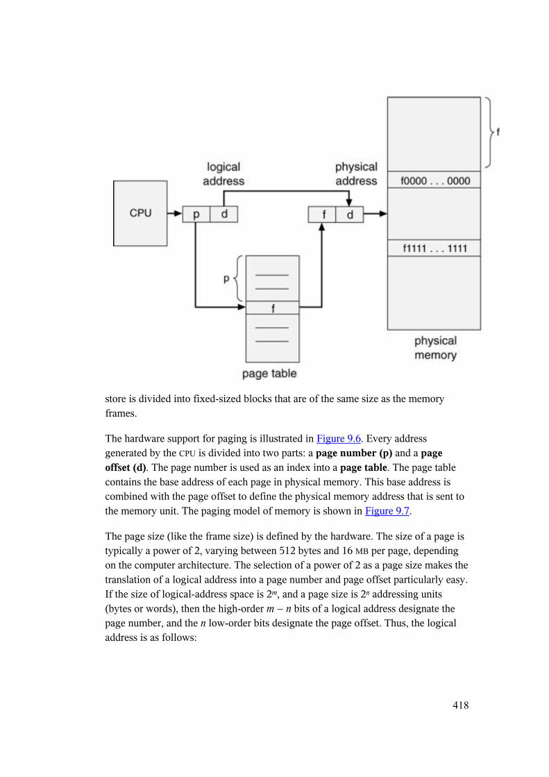
The hardware support for paging is illustrated in Figure 9.6. Every address generated by the CPU is divided into two parts: a page number (p) and a page offset (d). The page number is used as an index into a page table. The page table contains the base address of each page in physical memory. This base address is combined with the page offset to define the physical memory address that is sent to the memory unit. The paging model of memory is shown in Figure 9.7.

The page size (like the frame size) is defined by the hardware. The size of a page is typically a power of 2, varying between 512 bytes and 16 MB per page, depending on the computer architecture. The selection of a power of 2 as a page size makes the translation of a logical address into a page number and page offset particularly easy. If the size of logical-address space is 2m, and a page size is 2n addressing units (bytes or words), then the high-order m n bits of a logical address designate the page number, and the n low-order bits designate the page offset. Thus, the logical address is as follows:

419

Figure 9.7 Paging model of logical and physical memory.

where p is an index into the page table and d is the displacement within the page.

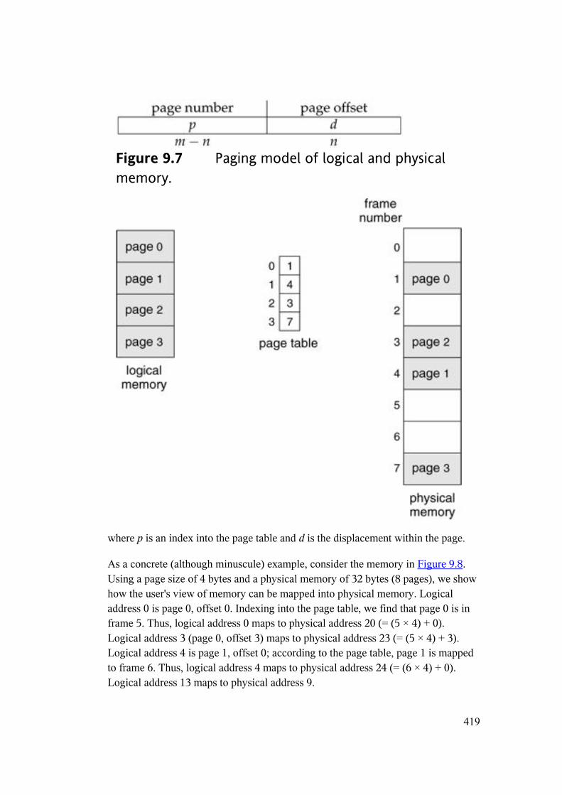
As a concrete (although minuscule) example, consider the memory in Figure 9.8. Using a page size of 4 bytes and a physical memory of 32 bytes (8 pages), we show how the user's view of memory can be mapped into physical memory. Logical address 0 is page 0, offset 0. Indexing into the page table, we find that page 0 is in frame 5. Thus, logical address 0 maps to physical address 20 (= (5 ! 4) + 0). Logical address 3 (page 0, offset 3) maps to physical address 23 (= (5 ! 4) + 3). Logical address 4 is page 1, offset 0; according to the page table, page 1 is mapped to frame 6. Thus, logical address 4 maps to physical address 24 (= (6 ! 4) + 0). Logical address 13 maps to physical address 9.

420

You may have noticed that paging itself is a form of dynamic relocation. Every logical address is bound by the paging hardware to some physical address. Using paging is similar to using a table of base (or relocation) registers, one for each frame of memory.

When we use a paging scheme, we have no external fragmentation: Any free frame can be allocated to a process that needs it. However, we may have some internal fragmentation. Notice that frames are allocated as units. If the memory requirements of a process do not happen to coincide with page boundaries, the lastframe allocated may not be completely full. For example, if page size is 2,048 bytes, a process of 72,766 bytes would need 35 pages plus 1,086 bytes. It would be allocated 36 frames, resulting in an internal fragmentation

Figure 9.8 Paging example for a 32-byte memory with 4-byte pages.

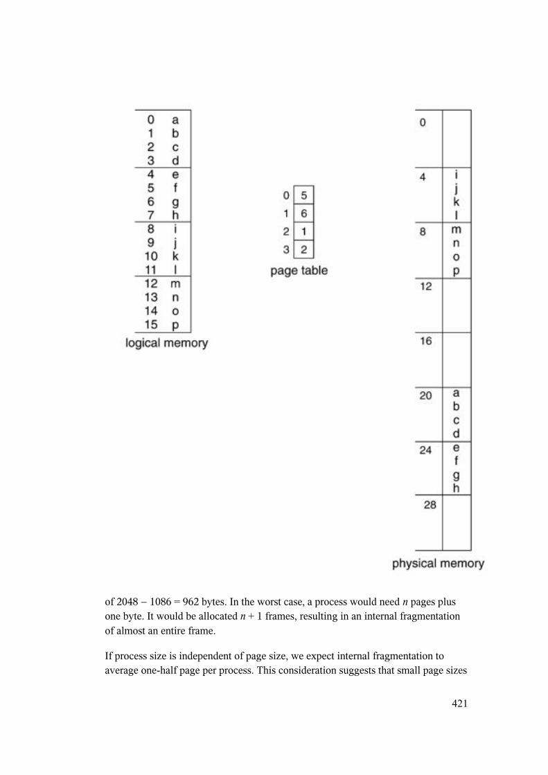
421

of 2048 1086 = 962 bytes. In the worst case, a process would need n pages plus one byte. It would be allocated n + 1 frames, resulting in an internal fragmentation of almost an entire frame.

If process size is independent of page size, we expect internal fragmentation to average one-half page per process. This consideration suggests that small page sizes

422

are desirable. However, overhead is involved in each page-table entry, and this overhead is reduced as the size of the pages increases. Also, disk I/O is more efficient when the number of data being transferred is larger (Chapter 14). Generally, page sizes have grown over time as processes, data sets, and main memory have beco me larger. Today, pages typically are between 4 KB and 8 KB in size, and some systems support even larger page sizes. Some CPUs and kernels even support multiple page sizes. For instance, Solaris uses page sizes of 8 KB and 4 MB, depending on the data stored by the pages. Researchers are now developing variable on-the-fly page-size support.

Usually, each page-table entry is 4 bytes long, but that size can vary as well. A 32-bit entry can point to one of 232 physical page frames. If frame size is 4 KB, then a system with 4-byte entries can address 244 bytes (or 16 TB) of physical memory.

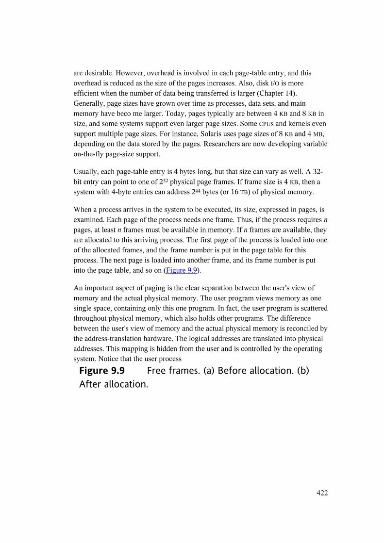
When a process arrives in the system to be executed, its size, expressed in pages, is examined. Each page of the process needs one frame. Thus, if the process requires npages, at least n frames must be available in memory. If n frames are available, they are allocated to this arriving process. The first page of the process is loaded into one of the allocated frames, and the frame number is put in the page table for this process. The next page is loaded into another frame, and its frame number is put into the page table, and so on (Figure 9.9).

An important aspect of paging is the clear separation between the user's view of memory and the actual physical memory. The user program views memory as one single space, containing only this one program. In fact, the user program is scattered throughout physical memory, which also holds other programs. The difference between the user's view of memory and the actual physical memory is reconciled by the address-translation hardware. The logical addresses are translated into physical addresses. This mapping is hidden from the user and is controlled by the operating system. Notice that the user process

Figure 9.9 Free frames. (a) Before allocation. (b) After allocation.

423

by definition is unable to access memory it does not own. It has no way of addressing memory outside of its page table, and the table includes only those pages that the process owns.

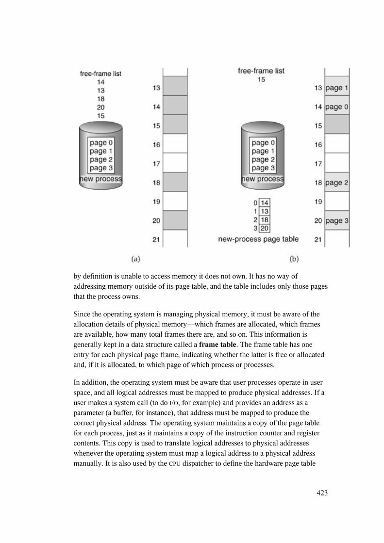
Since the operating system is managing physical memory, it must be aware of the allocation details of physical memory—which frames are allocated, which frames are available, how many total frames there are, and so on. This information is generally kept in a data structure called a frame table. The frame table has one entry for each physical page frame, indicating whether the latter is free or allocated and, if it is allocated, to which page of which process or processes.

In addition, the operating system must be aware that user processes operate in user space, and all logical addresses must be mapped to produce physical addresses. If a user makes a system call (to do I/O, for example) and provides an address as a parameter (a buffer, for instance), that address must be mapped to produce the correct physical address. The operating system maintains a copy of the page table for each process, just as it maintains a copy of the instruction counter and register contents. This copy is used to translate logical addresses to physical addresses whenever the operating system must map a logical address to a physical address manually. It is also used by the CPU dispatcher to define the hardware page table

424

when a process is to be allocated the CPU. Paging therefore increases the context-switch time.

9.4.2 Hardware Support

Each operating system has its own methods for storing page tables. Most allocate a page table for each process. A pointer to the page table is stored with the other register values (like the instruction counter) in the process control block. When the dispatcher is told to start a process, it must reload the user registers and define the correct hardware page-table values from the stored user page table.

The hardware implementation of the page table can be done in several ways. In the simplest case, the page table is implemented as a set of dedicated registers. These registers should be built with very high-speed logic to make the paging-address translation efficient. Every access to memory must go through the paging map, so efficiency is a major consideration. The CPU dispatcher reloads these registers, just as it reloads the other registers. Instructions to load or modify the page-table registers are, of course, privileged, so that only the operating system can change the memory map. The DEC PDP-11 is an example of such an architecture. The address consists of 16 bits, and the page size is 8 KB. The page table thus consists of eight entries that are kept in fast registers.

The use of registers for the page table is satisfactory if the page table is reasonably small (for example, 256 entries). Most contemporary computers, however, allow the page table to be very large (for example, 1 million entries). For these machines, the use of fast registers to implement the page table is not feasible. Rather, the page table is kept in main memory, and a page-table base register (PTBR) points to the page table. Changing page tables requires changing only this one register, substantially reducing context-switch time.

The problem with this approach is the time required to access a user memory location. If we want to access location i, we must first index into the page table, using the value in the PTBR offset by the page number for i. This task requires a memory access. It provides us with the frame number, which is combined with the page offset to produce the actual address. We can then access the desired place in memory. With this scheme, two memory accesses are needed to access a byte (one for the page-table entry, one for the byte). Thus, memory access is slowed by a factor of 2. This delay would be intolerable under most circumstances. We might as well resort to swapping!

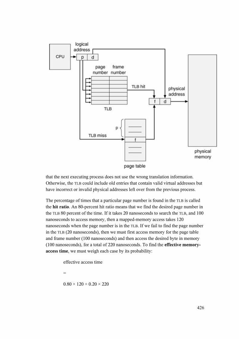
425

The standard solution to this problem is to use a special, small, fast-lookup hardware cache, called translation look-aside buffer (TLB). The TLB is associative, high-speed memory. Each entry in the TLB consists of two parts: a key (or tag) and a value. When the associative memory is presented with an item, the item is compared with all keys simultaneously. If the item is found, the corresponding value field is returned. The search is fast; the hardware, however, is expensive. Typically, the number of entries in a TLB is small, often numbering between 64 and 1,024.

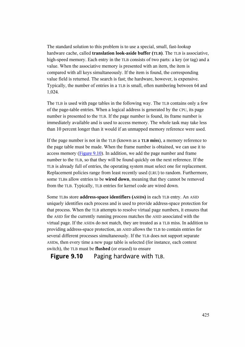
The TLB is used with page tables in the following way. The TLB contains only a few of the page-table entries. When a logical address is generated by the CPU, its page number is presented to the TLB. If the page number is found, its frame number is immediately available and is used to access memory. The whole task may take less than 10 percent longer than it would if an unmapped memory reference were used.

If the page number is not in the TLB (known as a TLB miss), a memory reference to the page table must be made. When the frame number is obtained, we can use it to access memory (Figure 9.10). In addition, we add the page number and frame number to the TLB, so that they will be found quickly on the next reference. If the TLB is already full of entries, the operating system must select one for replacement. Replacement policies range from least recently used (LRU) to random. Furthermore, some TLBs allow entries to be wired down, meaning that they cannot be removed from the TLB. Typically, TLB entries for kernel code are wired down.

Some TLBs store address-space identifiers (ASIDs) in each TLB entry. An ASID

uniquely identifies each process and is used to provide address-space protection for that process. When the TLB attempts to resolve virtual page numbers, it ensures that the ASID for the currently running process matches the ASID associated with the virtual page. If the ASIDs do not match, they are treated as a TLB miss. In addition to providing address-space protection, an ASID allows the TLB to contain entries for several different processes simultaneously. If the TLB does not support separate ASIDs, then every time a new page table is selected (for instance, each context switch), the TLB must be flushed (or erased) to ensure

Figure 9.10 Paging hardware with TLB.

426

that the next executing process does not use the wrong translation information. Otherwise, the TLB could include old entries that contain valid virtual addresses but have incorrect or invalid physical addresses left over from the previous process.

The percentage of times that a particular page number is found in the TLB is called the hit ratio. An 80-percent hit ratio means that we find the desired page number in the TLB 80 percent of the time. If it takes 20 nanoseconds to search the TLB, and 100nanoseconds to access memory, then a mapped-memory access takes 120nanoseconds when the page number is in the TLB. If we fail to find the page number in the TLB (20 nanoseconds), then we must first access memory for the page table and frame number (100 nanoseconds) and then access the desired byte in memory (100 nanoseconds), for a total of 220 nanoseconds. To find the effective memory-access time, we must weigh each case by its probability:

effective access time

=

0.80 ! 120 + 0.20 ! 220

427

=

140 nanoseconds.

In this example, we suffer a 40-percent slowdown in memory-access time (from 100 to 140 nanoseconds).

For a 98-percent hit ratio, we have

effective access time

=

0.98 ! 120 + 0.02 ! 220

=

122 nanoseconds.

This increased hit rate produces only a 22 percent slowdown in access time. We will further explore the impact of the hit ratio on the TLB in Chapter 10.

9.4.3 Protection

Memory protection in a paged environment is accomplished by protection bits associated with each frame. Normally, these bits are kept in the page table.

One bit can define a page to be read-write or read-only. Every reference to memory goes through the page table to find the correct frame number. At the same time that the physical address is being computed, the protection bits can be checked to verify that no writes are being made to a read-only page. An attempt to write to a read-only page causes a hardware trap to the operating system (or memory-protection violation).

We can easily expand this approach to provide a finer level of protection. We can create hardware to provide read-only, read-write, or execute-only protection; or, by providing separate protection bits for each kind of access, we can allow any combination of these accesses. Illegal attempts will be trapped to the operating system.

One more bit is generally attached to each entry in the page table: a valid-invalidbit. When this bit is set to "valid," the associated page is in the process's logical-address space and is thus a legal (or valid) page. When the bit is set to "invalid," the

428

page is not in the process's logical-address space. Illegal addresses are trapped by use of the valid-invalid bit. The operating system sets this bit for each page to allow or disallow accesses to the page.

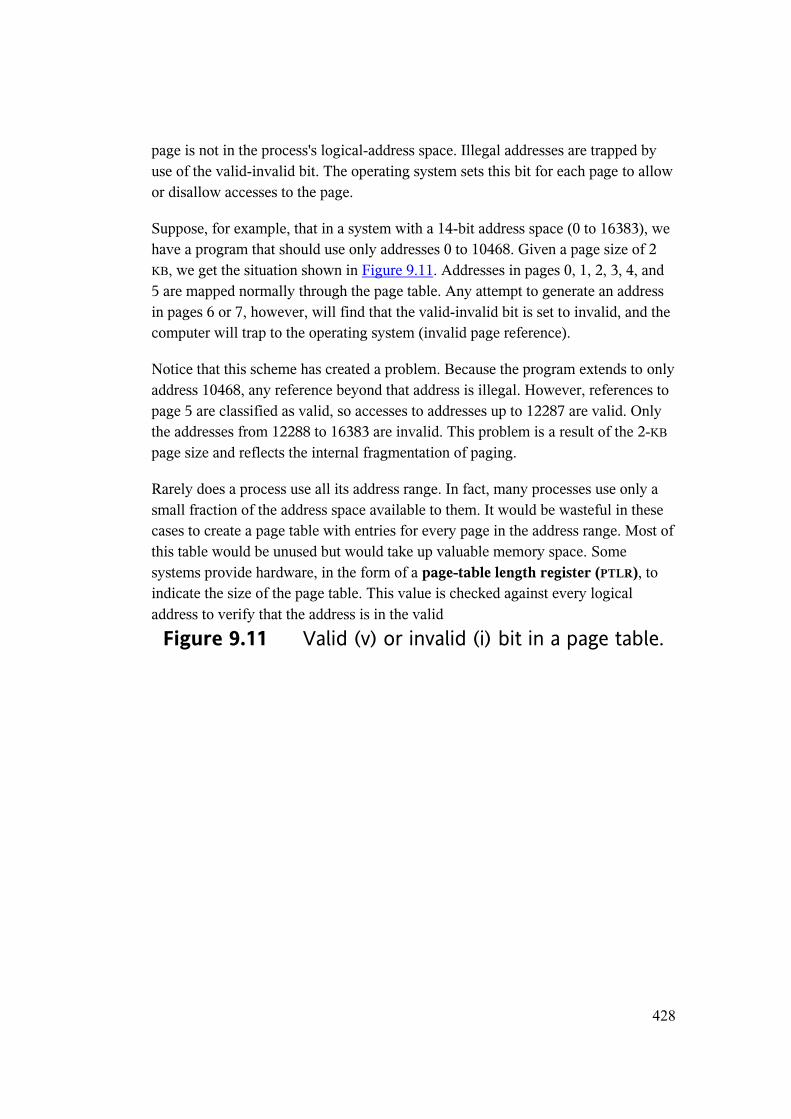
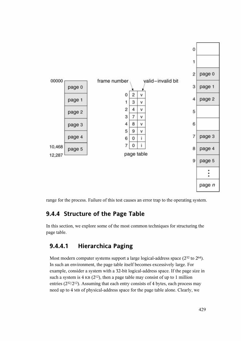
Suppose, for example, that in a system with a 14-bit address space (0 to 16383), we have a program that should use only addresses 0 to 10468. Given a page size of 2KB, we get the situation shown in Figure 9.11. Addresses in pages 0, 1, 2, 3, 4, and 5 are mapped normally through the page table. Any attempt to generate an address in pages 6 or 7, however, will find that the valid-invalid bit is set to invalid, and the computer will trap to the operating system (invalid page reference).

Notice that this scheme has created a problem. Because the program extends to only address 10468, any reference beyond that address is illegal. However, references to page 5 are classified as valid, so accesses to addresses up to 12287 are valid. Only the addresses from 12288 to 16383 are invalid. This problem is a result of the 2-KB

page size and reflects the internal fragmentation of paging.

Rarely does a process use all its address range. In fact, many processes use only a small fraction of the address space available to them. It would be wasteful in these cases to create a page table with entries for every page in the address range. Most of this table would be unused but would take up valuable memory space. Some systems provide hardware, in the form of a page-table length register (PTLR), to indicate the size of the page table. This value is checked against every logical address to verify that the address is in the valid

Figure 9.11 Valid (v) or invalid (i) bit in a page table.

429

range for the process. Failure of this test causes an error trap to the operating system.

9.4.4 Structure of the Page Table

In this section, we explore some of the most common techniques for structuring the page table.

9.4.4.1 Hierarchica Paging

Most modern computer systems support a large logical-address space (232 to 264). In such an environment, the page table itself becomes excessively large. For example, consider a system with a 32-bit logical-address space. If the page size in such a system is 4 KB (212), then a page table may consist of up to 1 million entries (232/212). Assuming that each entry consists of 4 bytes, each process may need up to 4 MB of physical-address space for the page table alone. Clearly, we

430

would not want to allocate the page table contiguously in main memory. One simple solution to this problem is to divide the page table into smaller pieces. We can accomplish this division in several ways.

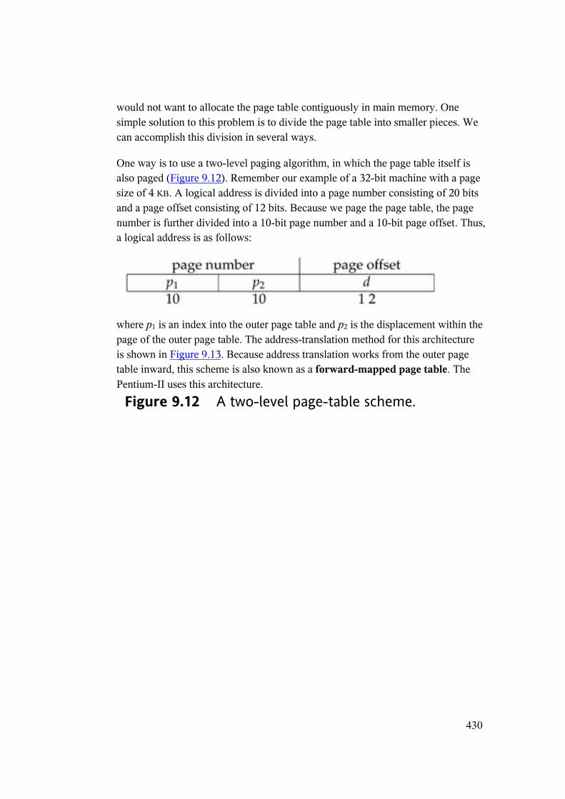
One way is to use a two-level paging algorithm, in which the page table itself is also paged (Figure 9.12). Remember our example of a 32-bit machine with a page size of 4 KB. A logical address is divided into a page number consisting of 20 bits and a page offset consisting of 12 bits. Because we page the page table, the page number is further divided into a 10-bit page number and a 10-bit page offset. Thus, a logical address is as follows:

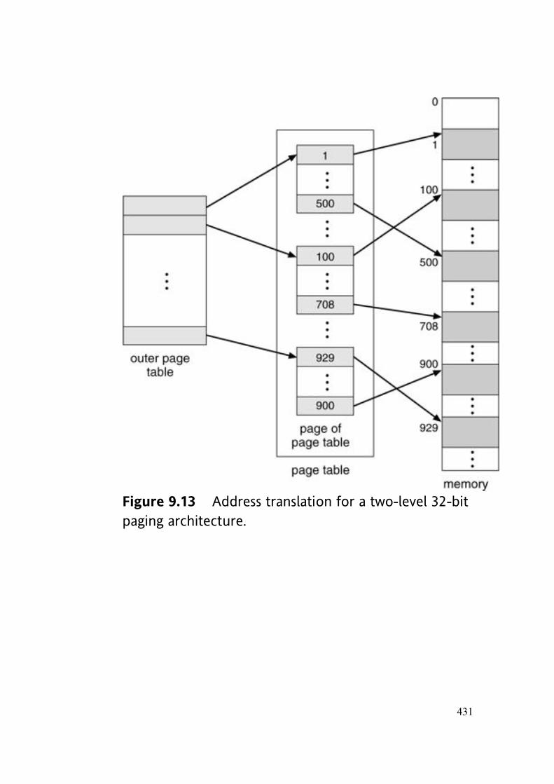
where p1 is an index into the outer page table and p2 is the displacement within the page of the outer page table. The address-translation method for this architecture is shown in Figure 9.13. Because address translation works from the outer page table inward, this scheme is also known as a forward-mapped page table. The Pentium-II uses this architecture.

Figure 9.12 A two-level page-table scheme.

431

Figure 9.13 Address translation for a two-level 32-bit paging architecture.

432

The VAX architecture also supports a variation of two-level paging. The VAX is a 32-bit machine with a page size of 512 bytes. The logical-address space of a process is divided into four equal sections, each of which consists of 230 bytes. Each section represents a different part of the logical-address space of a process. The first 2 high-order bits of the logical address designate the appropriate section. The next 21 bits represent the logical page number of that section, and the final 9bits represent an offset in the desired page. By partitioning the page table in this manner, the operating system can leave partitions unused until a process needs them. An address on the VAX architecture is as follows:

where s designates the section number, p is an index into the page table, and d is the displacement within the page.

Even when this scheme is used, the size of a one-level page table for a VAX

process using one section still is 221 bits * 4 bytes per entry = MB. So that main-memory use is reduced even further, the VAX pages the user-process page tables.

For a system with a 64-bit logical-address space, a two-level paging scheme is no longer appropriate. To illustrate this point, let us suppose that the page size in such a system is 4 KB (212). In this case, the page table will consist of up to 252

entries. If we use a two-level paging scheme, then the inner page tables could conveniently be one page long, or contain 210 4-byte entries. The addresses would look like this:

433

The outer page table will consist of 242 entries, or 244 bytes. The obvious method to avoid such a large table is to divide the outer page table into smaller pieces. This approach is also used on some 32-bit processors for added flexibility and efficiency.

We can divide the outer page table in various ways. We can page the outer page table, giving us a three-level paging scheme. Suppose that the outer page table is made up of standard-size pages (210 entries, or 212 bytes); a 64-bit address space is still daunting:

The outer page table is still 234 bytes in size.

The next step would be a four-level paging scheme, where the second-level outer page table itself is also paged. The SPARC architecture (with 32-bit addressing) supports a three-level paging scheme, whereas the 32-bit Motorola 68030architecture supports a four-level paging scheme.

For 64-bit architectures, hierarchical page tables are generally considered inappropriate. For example, the 64-bit UltraSPARC would require seven levels of paging—a prohibitive number of memory accesses to translate each logical address.

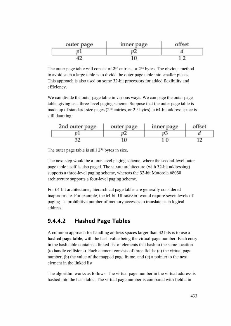
9.4.4.2 Hashed Page Tables

A common approach for handling address spaces larger than 32 bits is to use a hashed page table, with the hash value being the virtual-page number. Each entry in the hash table contains a linked list of elements that hash to the same location (to handle collisions). Each element consists of three fields: (a) the virtual page number, (b) the value of the mapped page frame, and (c) a pointer to the next element in the linked list.

The algorithm works as follows: The virtual page number in the virtual address is hashed into the hash table. The virtual page number is compared with field a in

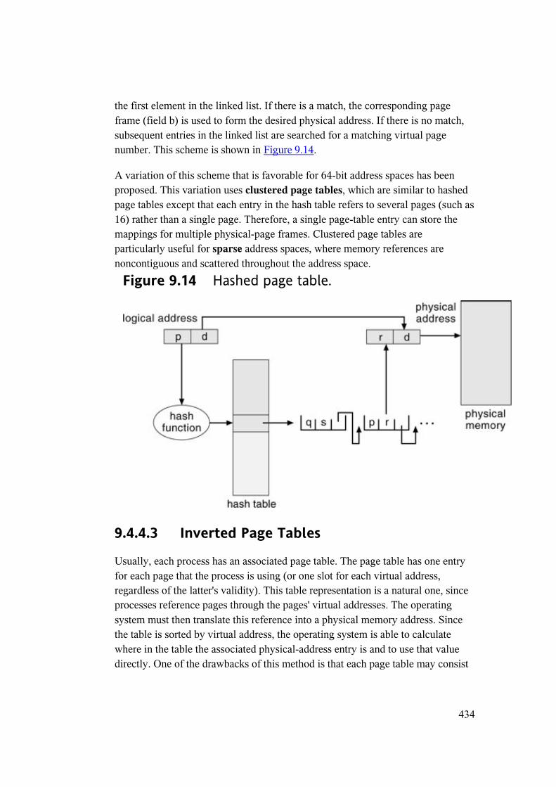
434

the first element in the linked list. If there is a match, the corresponding page frame (field b) is used to form the desired physical address. If there is no match, subsequent entries in the linked list are searched for a matching virtual page number. This scheme is shown in Figure 9.14.

A variation of this scheme that is favorable for 64-bit address spaces has been proposed. This variation uses clustered page tables, which are similar to hashed page tables except that each entry in the hash table refers to several pages (such as 16) rather than a single page. Therefore, a single page-table entry can store the mappings for multiple physical-page frames. Clustered page tables are particularly useful for sparse address spaces, where memory references are noncontiguous and scattered throughout the address space.

Figure 9.14 Hashed page table.

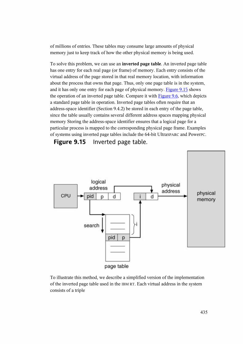
9.4.4.3 Inverted Page Tables

Usually, each process has an associated page table. The page table has one entry for each page that the process is using (or one slot for each virtual address, regardless of the latter's validity). This table representation is a natural one, since processes reference pages through the pages' virtual addresses. The operating system must then translate this reference into a physical memory address. Since the table is sorted by virtual address, the operating system is able to calculate where in the table the associated physical-address entry is and to use that value directly. One of the drawbacks of this method is that each page table may consist

435

of millions of entries. These tables may consume large amounts of physical memory just to keep track of how the other physical memory is being used.

To solve this problem, we can use an inverted page table. An inverted page table has one entry for each real page (or frame) of memory. Each entry consists of the virtual address of the page stored in that real memory location, with information about the process that owns that page. Thus, only one page table is in the system, and it has only one entry for each page of physical memory. Figure 9.15 shows the operation of an inverted page table. Compare it with Figure 9.6, which depicts a standard page table in operation. Inverted page tables often require that an address-space identifier (Section 9.4.2) be stored in each entry of the page table, since the table usually contains several different address spaces mapping physical memory Storing the address-space identifier ensures that a logical page for a particular process is mapped to the corresponding physical page frame. Examples of systems using inverted page tables include the 64-bit UltraSPARC and PowerPC.

Figure 9.15 Inverted page table.

To illustrate this method, we describe a simplified version of the implementation of the inverted page table used in the IBM RT. Each virtual address in the system consists of a triple

436

<process-id, page-number, offset>.

Each inverted page-table entry is a pair <process-id, page-number> where the process-id assumes the role of the address-space identifier. When a memory reference occurs, part of the virtual address, consisting of <process-id, page-number>, is presented to the memory subsystem. The inverted page table is then searched for a match. If a match is found—say, at entry i—then the physical address <i, offset> is generated. If no match is found, then an illegal address access has been attempted.

Although this scheme decreases the amount of memory needed to store each page table, it increases the amount of time needed to search the table when a page reference occurs. Because the inverted page table is sorted by physical address, but lookups occur on virtual addresses, the whole table might need to be searched for a match. This search would take far too long. To alleviate this problem, we use a hash table, as described in Section 9.4.4.2, to limit the search to one—or at most a few—page-table entries. Of course, each access to the hash table adds a memory reference to the procedure, so one virtual-memory reference requires at least two real-memory reads: one for the hash-table entry and one for the page table. To improve performance, recall that the TLB is searched first, before the hash table is consulted.

9.4.5 Shared Pages

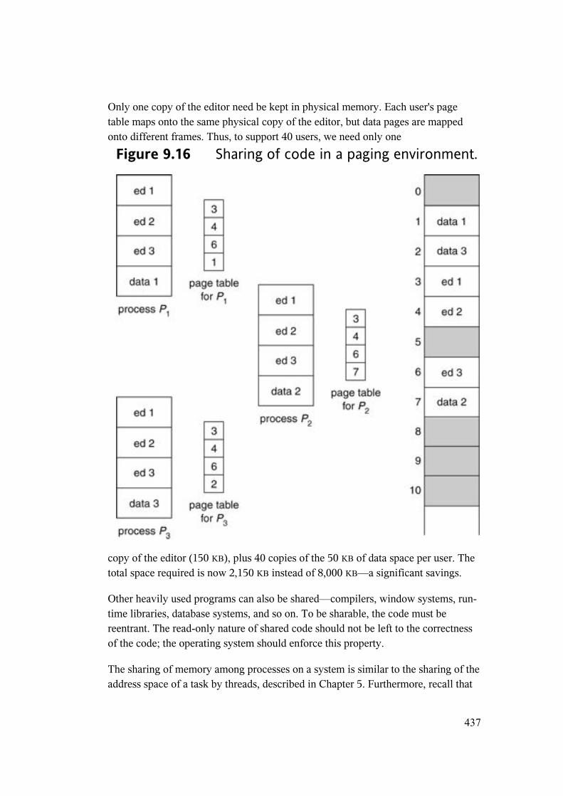
Another advantage of paging is the possibility of sharing common code. This consideration is particularly important in a time-sharing environment. Consider a system that supports 40 users, each of whom executes a text editor. If the text editor consists of 150 KB of code and 50 KB of data space, we need 8,000 KB to support the 40 users. If the code is reentrant code (or pure code), however, it can be shared, as shown in Figure 9.16. Here we see a three-page editor—each page 50 KB in size (the large page size is used to simplify the figure)—being shared among three processes. Each process has its own data page.

Reentrant code is non-self-modifying code; it never changes during execution. Thus, two or more processes can execute the same code at the same time. Each process has its own copy of registers and data storage to hold the data for the process's execution. The data for two different processes will, of course, vary for each process.

437

Only one copy of the editor need be kept in physical memory. Each user's page table maps onto the same physical copy of the editor, but data pages are mapped onto different frames. Thus, to support 40 users, we need only one

Figure 9.16 Sharing of code in a paging environment.

copy of the editor (150 KB), plus 40 copies of the 50 KB of data space per user. The total space required is now 2,150 KB instead of 8,000 KB—a significant savings.

Other heavily used programs can also be shared—compilers, window systems, run-time libraries, database systems, and so on. To be sharable, the code must be reentrant. The read-only nature of shared code should not be left to the correctness of the code; the operating system should enforce this property.

The sharing of memory among processes on a system is similar to the sharing of the address space of a task by threads, described in Chapter 5. Furthermore, recall that

438

in Chapter 4 we described shared memory as a method of interprocess communication. Some operating systems implement shared memory using shared pages.

Systems that use inverted page tables have difficulty implementing shared memory. Shared memory is usually implemented as multiple virtual addresses (one for each process sharing the memory) that are mapped to one physical address. This standard method cannot be used with inverted page tables; because there is only one virtual page entry for every physical page, one physical page cannot have two (or more) shared virtual addresses.

Organizing memory according to pages provides numerous benefits in addition to allowing several processes to share the same physical pages. We will cover several other benefits in Chapter 10.

9.5 Segmentation

An important aspect of memory management that became unavoidable with paging is the separation of the user's view of memory and the actual physical memory. As we have already seen, the user's view of memory is not the same as the actual physical memory. The user's view is mapped onto physical memory. This mapping allows differentiation between logical memory and physical memory.

9.5.1 Basic Method

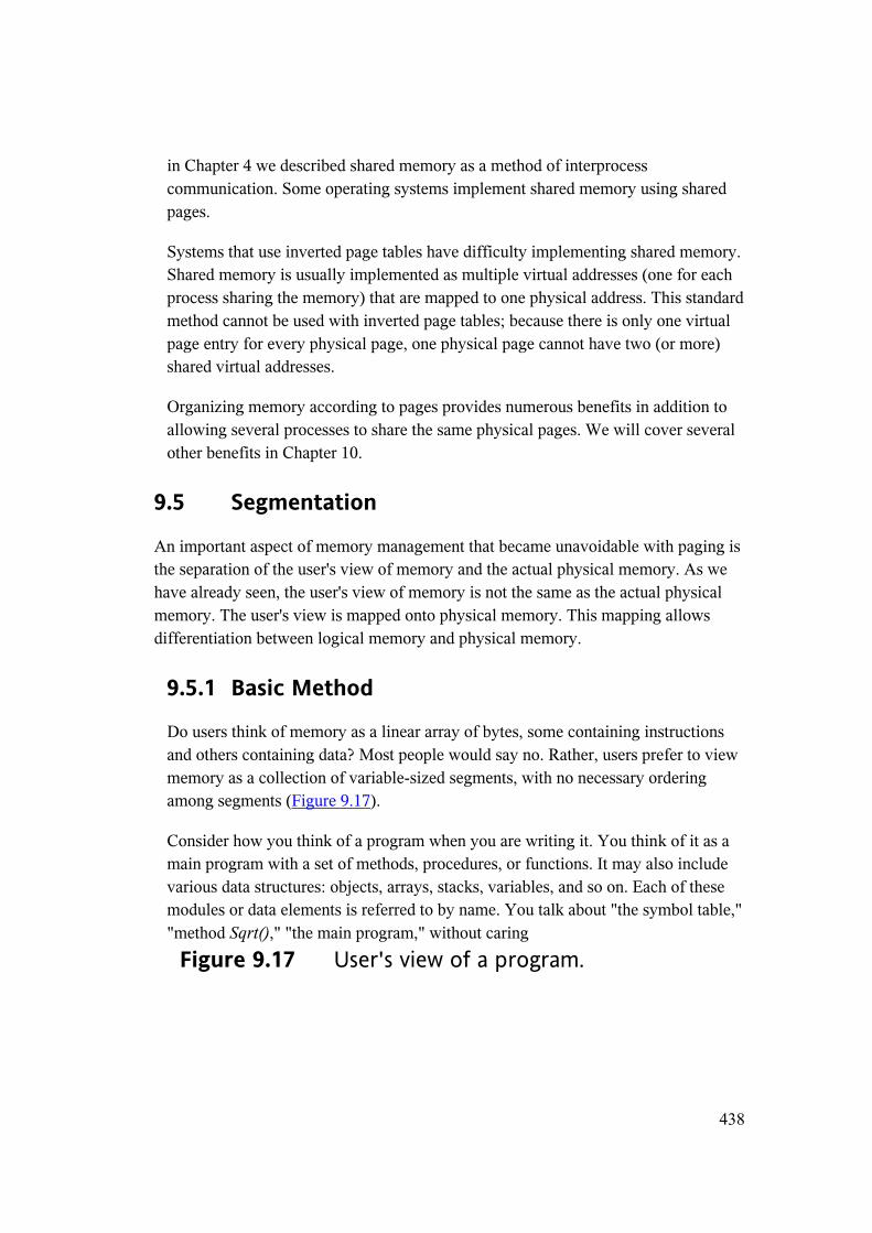
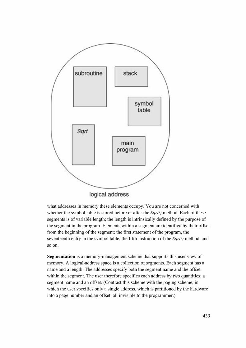
Do users think of memory as a linear array of bytes, some containing instructions and others containing data? Most people would say no. Rather, users prefer to view memory as a collection of variable-sized segments, with no necessary ordering among segments (Figure 9.17).

Consider how you think of a program when you are writing it. You think of it as a main program with a set of methods, procedures, or functions. It may also include various data structures: objects, arrays, stacks, variables, and so on. Each of these modules or data elements is referred to by name. You talk about "the symbol table," "method Sqrt()," "the main program," without caring

Figure 9.17 User's view of a program.

439

what addresses in memory these elements occupy. You are not concerned with whether the symbol table is stored before or after the Sqrt() method. Each of these segments is of variable length; the length is intrinsically defined by the purpose of the segment in the program. Elements within a segment are identified by their offset from the beginning of the segment: the first statement of the program, the seventeenth entry in the symbol table, the fifth instruction of the Sqrt() method, and so on.

Segmentation is a memory-management scheme that supports this user view of memory. A logical-address space is a collection of segments. Each segment has a name and a length. The addresses specify both the segment name and the offset within the segment. The user therefore specifies each address by two quantities: a segment name and an offset. (Contrast this scheme with the paging scheme, in which the user specifies only a single address, which is partitioned by the hardware into a page number and an offset, all invisible to the programmer.)

440

For simplicity of implementation, segments are numbered and are referred to by a segment number, rather than by a segment name. Thus, a logical address consists of a two tuple:

<segment-number, offset>.

Normally, the user program is compiled, and the compiler automatically constructs segments reflecting the input program. A Java compiler might create separate segments for the following:

1. The method area, which holds the code for all methods

2. The heap, from which memory for objects is allocated

3. The stacks used by each Java thread

4. The class loader

A C compiler might create a separate segment for global variables. Libraries that are linked in during compile time might be assigned separate segments. The loader would take all these segments and assign them segment numbers.

9.5.2 Hardware

Although the user can now refer to objects in the program by a two-dimensional address, the actual physical memory is still, of course, a one-dimensional sequence of bytes. Thus, we must define an implementation to map two-dimensional user-defined addresses into one-dimensional physical addresses. This mapping is effected by a segment table. Each entry in the segment table

Figure 9.18 Segmentation hardware.

441

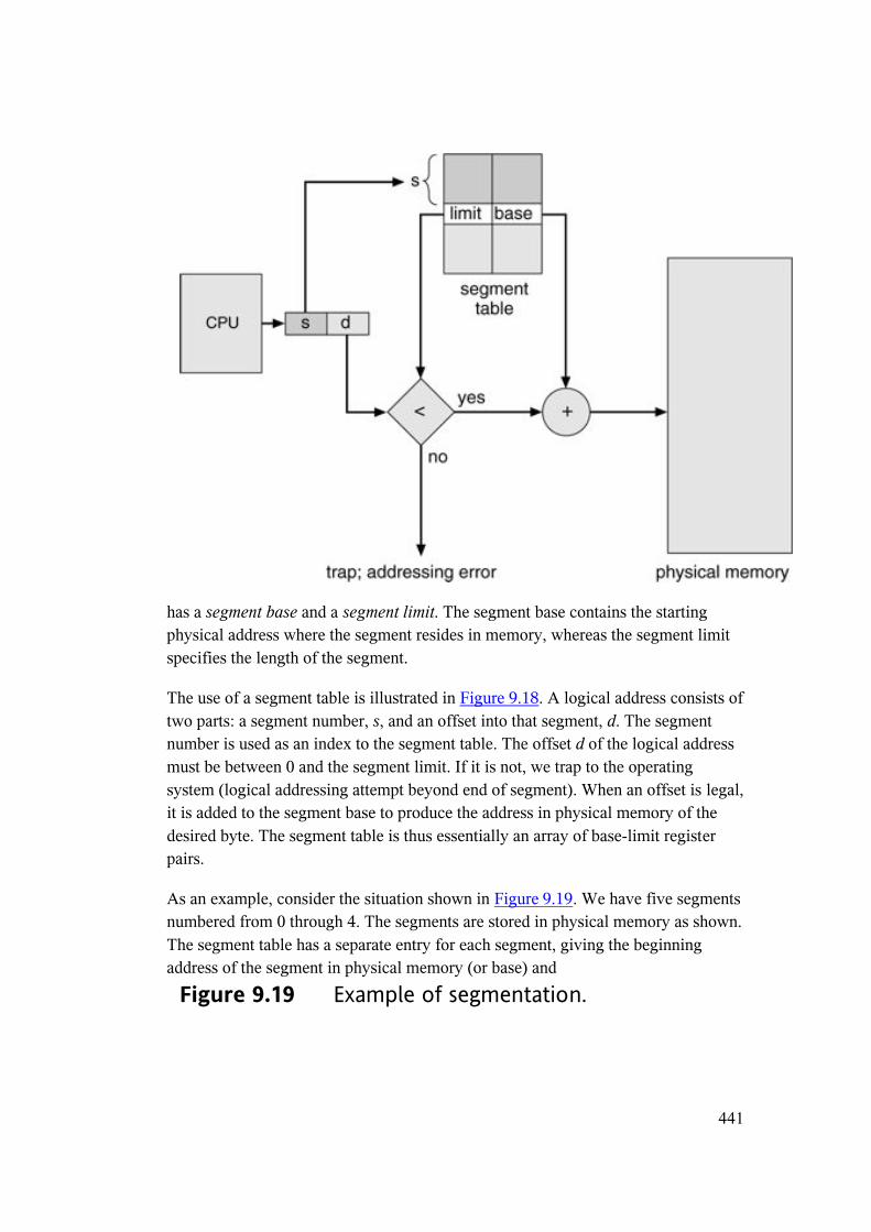
has a segment base and a segment limit. The segment base contains the starting physical address where the segment resides in memory, whereas the segment limit specifies the length of the segment.

The use of a segment table is illustrated in Figure 9.18. A logical address consists of two parts: a segment number, s, and an offset into that segment, d. The segment number is used as an index to the segment table. The offset d of the logical address must be between 0 and the segment limit. If it is not, we trap to the operating system (logical addressing attempt beyond end of segment). When an offset is legal, it is added to the segment base to produce the address in physical memory of the desired byte. The segment table is thus essentially an array of base-limit register pairs.

As an example, consider the situation shown in Figure 9.19. We have five segments numbered from 0 through 4. The segments are stored in physical memory as shown. The segment table has a separate entry for each segment, giving the beginning address of the segment in physical memory (or base) and

Figure 9.19 Example of segmentation.

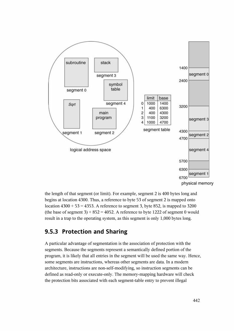
442

the length of that segment (or limit). For example, segment 2 is 400 bytes long and begins at location 4300. Thus, a reference to byte 53 of segment 2 is mapped onto location 4300 + 53 = 4353. A reference to segment 3, byte 852, is mapped to 3200(the base of segment 3) + 852 = 4052. A reference to byte 1222 of segment 0 would result in a trap to the operating system, as this segment is only 1,000 bytes long.

9.5.3 Protection and Sharing

A particular advantage of segmentation is the association of protection with the segments. Because the segments represent a semantically defined portion of the program, it is likely that all entries in the segment will be used the same way. Hence, some segments are instructions, whereas other segments are data. In a modern architecture, instructions are non-self-modifying, so instruction segments can be defined as read-only or execute-only. The memory-mapping hardware will check the protection bits associated with each segment-table entry to prevent illegal

443

accesses to memory, such as attempts to write into a read-only segment or to use an execute-only segment as data. By placing an array in its own segment, the memory-management hardware will automatically check that array indexes are legal and do not stray outside the array boundaries. Thus, many common program errors will be detected by the hardware before they can cause serious damage.

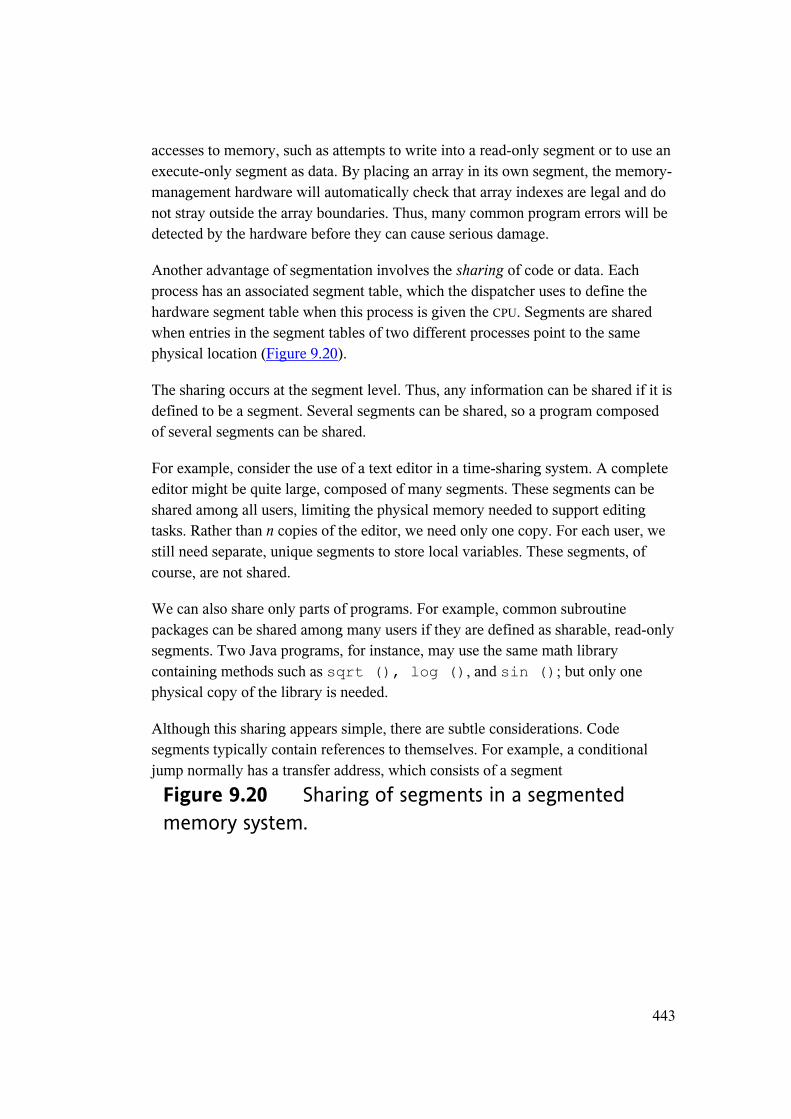
Another advantage of segmentation involves the sharing of code or data. Each process has an associated segment table, which the dispatcher uses to define the hardware segment table when this process is given the CPU. Segments are shared when entries in the segment tables of two different processes point to the same physical location (Figure 9.20).

The sharing occurs at the segment level. Thus, any information can be shared if it is defined to be a segment. Several segments can be shared, so a program composed of several segments can be shared.

For example, consider the use of a text editor in a time-sharing system. A complete editor might be quite large, composed of many segments. These segments can be shared among all users, limiting the physical memory needed to support editing tasks. Rather than n copies of the editor, we need only one copy. For each user, we still need separate, unique segments to store local variables. These segments, of course, are not shared.

We can also share only parts of programs. For example, common subroutine packages can be shared among many users if they are defined as sharable, read-only segments. Two Java programs, for instance, may use the same math library containing methods such as sqrt (), log (), and sin (); but only one physical copy of the library is needed.

Although this sharing appears simple, there are subtle considerations. Code segments typically contain references to themselves. For example, a conditional jump normally has a transfer address, which consists of a segment

Figure 9.20 Sharing of segments in a segmented memory system.

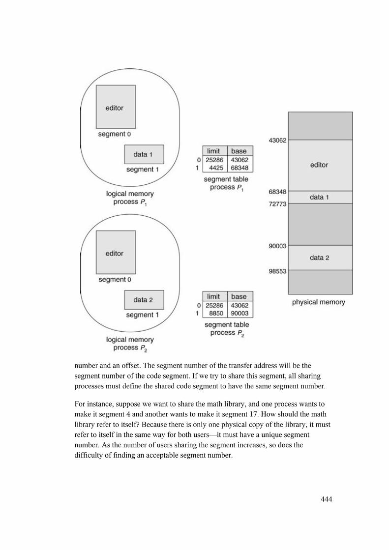
444

number and an offset. The segment number of the transfer address will be the segment number of the code segment. If we try to share this segment, all sharing processes must define the shared code segment to have the same segment number.

For instance, suppose we want to share the math library, and one process wants to make it segment 4 and another wants to make it segment 17. How should the math library refer to itself? Because there is only one physical copy of the library, it must refer to itself in the same way for both users—it must have a unique segment number. As the number of users sharing the segment increases, so does the difficulty of finding an acceptable segment number.

445

Read-only data segments that contain no physical pointers may be shared as different segment numbers, as may code segments that refer to themselves only indirectly. For example, conditional branches that specify the branch address as an offset from the current program counter or relative to a register containing the current segment number would allow code to avoid direct reference to the current segment number.

9.5.4 Fragmentation

The long-term scheduler must find and allocate memory for all the segments of a user program. This situation is similar to paging except that the segments are of variable length, whereas pages are all the same size. Thus, as with the variable-sized partition scheme, memory allocation is a dynamic storage-allocation problem, usually solved with a best-fit or first-fit algorithm.

It follows that segmentation may cause external fragmentation. When all blocks of free memory are too small to accommodate a segment, the process may simply have to wait until more memory (or at least a larger hole) becomes available or until compaction creates a larger hole. Because segmentation is by its nature a dynamic-relocation algorithm, we can compact memory whenever we want. If the CPU

scheduler must wait for one process because of a memory-allocation problem, it may (or may not) skip through the CPU queue looking for a smaller, lower-priority process to run.

How serious a problem is external fragmentation for a segmentation scheme? Would long-term scheduling with compaction help? The answers depend mainly on the average segment size. At one extreme, we could define each process to be one segment. This approach is analogous to the variable-sized partition scheme. At the other extreme, every byte could be put in its own segment and relocated separately. This arrangement eliminates external fragmentation altogether; however, every byte would need a base register for its relocation, doubling memory use! Of course, the next logical step—fixed-sized, small segments—is paging.

Generally, if the average segment size is small, external fragmentation will also be small. (By analogy, consider putting suitcases in the trunk of a car; they never quite seem to fit. However, if you open the suitcases and put the individual items in the trunk, everything is more likely to fit.) Because the individual segments are smaller than the overall process, they are more likely to fit in the available memory blocks.

9.6 Segmentation with Paging

446

Both paging and segmentation have advantages and disadvantages. In fact, of the two most popular microprocessors now being used, one—the Motorola 68000 line—is based on a flat-address space, whereas the other—the Intel 80x86 and Pentium family—is based on segmentation. Both are merging memory models toward a mixture of paging and segmentation. We can combine these two methods to improve on each. This combination is best illustrated by the architecture of the Intel 80x86.

The 80x86 uses segmentation with paging for memory management. The maximum number of segments per process is 16 KB, and each segment can be as large as 4gigabytes. The page size is 4 KB. We do not give a complete description of the memory-management structure of the 80x86 in this text. Rather, we present the major ideas.

The logical-address space of a process is divided into two partitions. The first partition consists of up to 8 KB segments that are private to that process. The second partition consists of up to 8 KB segments that are shared among all the processes. Information about the first partition is kept in the local descriptor table (LDT); information about the second partition is kept in the global descriptor table (GDT). Each entry in the LDT and GDT consists of an 8-byte segment descriptor with detailed information about a particular segment, including the base location and limit of that segment.

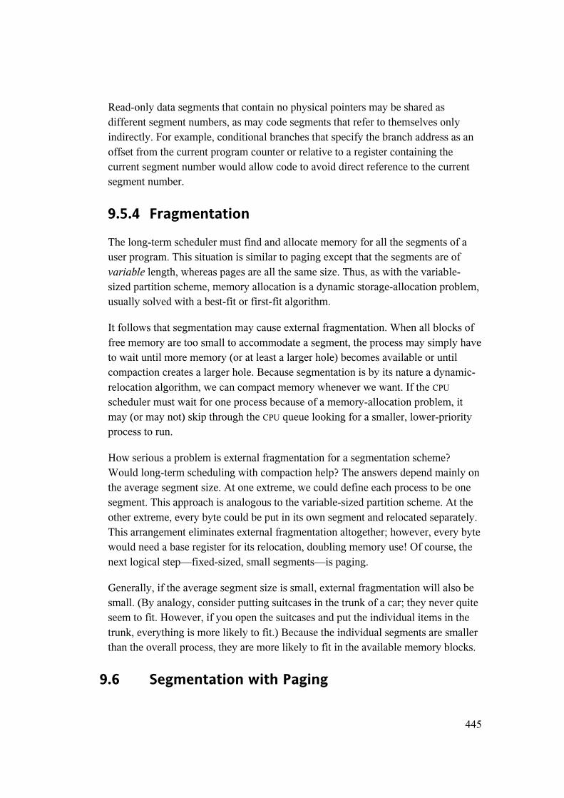
The logical address is a pair (selector, offset), where the selector is a 16-bit number:

in which s designates the segment number, g indicates whether the segment is in the GDT or LDT, and p deals with protection. The offset is a 32-bit number specifying the location of the byte (or word) within the segment in question.

The machine has six segment registers, allowing six segments to be addressed at any one time by a process. It has six 8-byte microprogram registers to hold the corresponding descriptors from either the LDT or GDT. This cache lets the 80x86 avoid having to read the descriptor from memory for every memory reference.

The physical address on the 80x86 is 32 bits long and is formed as follows. The segment register points to the appropriate entry in the LDT or GDT. The base and limit information about the segment in question is used to generate a linear address. First, the limit is used to check for address validity. If the address is not valid, a memory fault is generated, resulting in a trap to the operating system. If it is valid, then the

447

value of the offset is added to the value of the base, resulting in a 32-bit linear address. This address is then translated into a physical address.

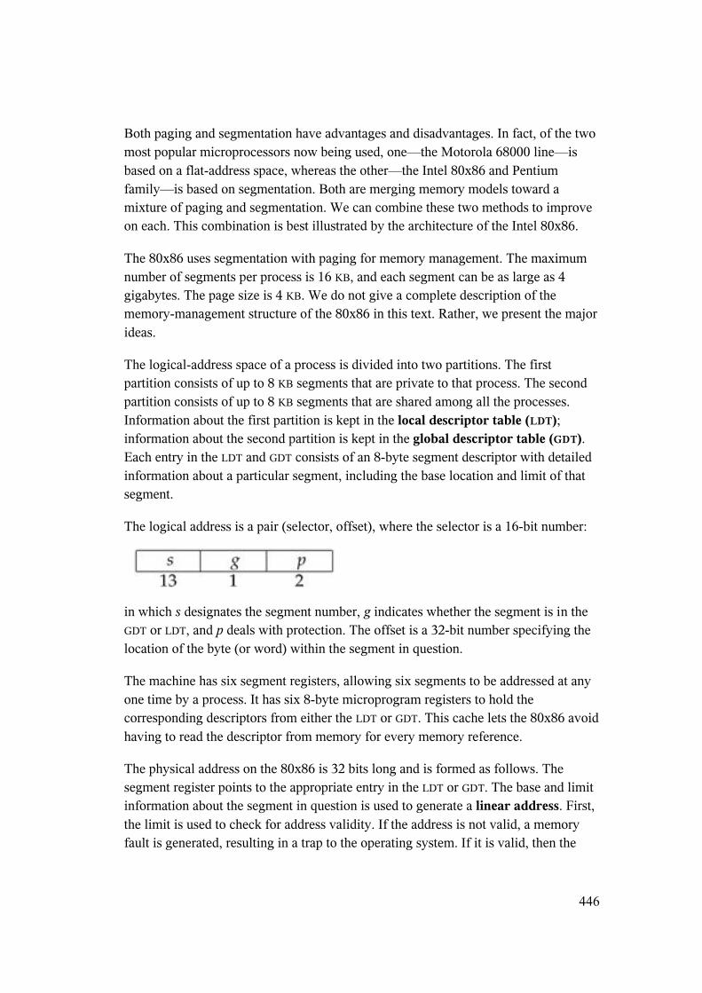
As pointed out previously, each segment is paged, and each page is 4 KB. A page table may thus consist of up to 1 million entries. Because each entry consists of 4bytes, each process may need up to 4 MB of physical-address space for the page table alone. Clearly, we would not want to allocate the page table contiguously in main memory. The solution adopted in the 80x86 is to use a two-level paging scheme. The linear address is divided into a page number consisting of 20 bits and a page offset consisting of 12 bits. Since we page the page table, the page number is further divided into a 10-bit page directory pointer and a 10-bit page table pointer. The logical address is as follows:

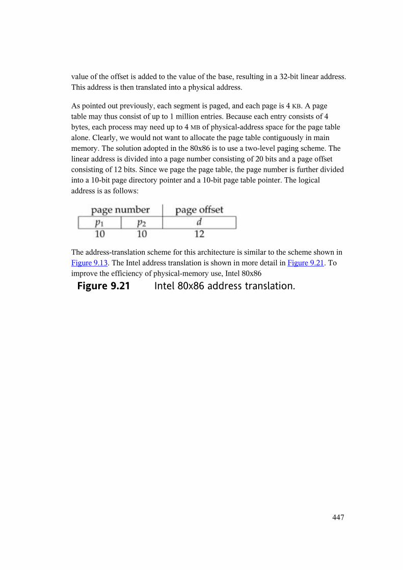
The address-translation scheme for this architecture is similar to the scheme shown in Figure 9.13. The Intel address translation is shown in more detail in Figure 9.21. To improve the efficiency of physical-memory use, Intel 80x86

Figure 9.21 Intel 80x86 address translation.

448

page tables can be swapped to disk. In this case, an invalid bit is used in the page-directory entry to indicate whether the table to which the entry is pointing is in memory or on disk. If the table is on disk, the operating system can use the other 31bits to specify the disk location of the table; the table then can be brought into memory on demand.

As an illustration, consider the Linux operating system running on the Intel 80x86architecture. Because Linux is designed to run on a variety of processors—many of which may provide only limited support for segmentation—Linux does not rely on segmentation and uses it minimally. On the Intel 80x86, Linux uses only six segments:

1. A segment for kernel code

449

2. A segment for kernel data

3. A segment for user code

4. A segment for user data

5. A task-state segment (TSS)

6. A default LDT segment

The segments for user code and user data are shared by all processes running in user mode. This is possible because all processes use the same logical address space and all segment descriptors are stored in the global descriptor table (GDT). Furthermore, each process has its own task-state segment (TSS), and the descriptor for this segment is stored in the GDT. The TSS is used to store the hardware context of each process during context switches. The default LDT segment is normally shared by all processes and is usually not used. However, if a process requires its own LDT, it can create one and use that instead of the default LDT.

As noted, each segment selector includes a 2-bit field for protection. Thus, the 80x86allows four levels of protection. Of these four levels, Linux only recognizes two: user mode and kernel mode.

9.7 Summary

Memory-management algorithms for multiprogrammed operating systems range from the simple single-user system approach to paged segmentation. The most important determinant of the method used in a particular system is the hardware provided. Every memory address generated by the CPU must be checked for legality and possibly mapped to a physical address. The checking cannot be implemented (efficiently) in software. Hence, we are constrained by the hardware available.

The memory-management algorithms discussed (contiguous allocation, paging, segmentation, and combinations of paging and segmentation) differ in many aspects. In comparing different memory-management strategies, we use the following considerations:

• Hardware support: A simple base register or a pair of base and limit registers is sufficient for the single- and multiple-partition schemes, whereas paging and segmentation need mapping tables to define the address map.

450

• Performance: As the memory-management algorithm becomes more complex, the time required to map a logical address to a physical address increases. For the simple systems, we need only compare or add to the logical address—operations that are fast. Paging and segmentation can be as fast if the table is implemented in fast registers. If the table is in memory, however, user memory accesses can be degraded substantially. A TLB can reduce the performance degradation to an acceptable level.

• Fragmentation: A multiprogrammed system will generally perform more efficiently if it has a higher level of multiprogramming. For a given set of processes, we can increase the multiprogramming level only by packing more processes into memory. To accomplish this task, we must reduce memory waste, or fragmentation. Systems with fixed-sized allocation units, such as the single-partition scheme and paging, suffer from internal fragmentation. Systems with variable-sized allocation units, such as the multiple-partition scheme and segmentation, suffer from external fragmentation.

• Relocation: One solution to the external-fragmentation problem is compaction. Compaction involves shifting a program in memory in such a way that the program does not notice the change. This consideration requires that logical addresses be relocated dynamically, at execution time. If addresses are relocated only at load time, we cannot compact storage.

• Swapping: Swapping can be added to any algorithm. At intervals determined by the operating system, usually dictated by CPU-scheduling policies, processes are copied from main memory to a backing store and later are copied back to main memory. This scheme allows more processes to be run than can be fit into memory at one time.

• Sharing: Another means of increasing the multiprogramming level is to share code and data among different users. Sharing generally requires that either paging or segmentation be used, to provide small packets of information (pages or segments) that can be shared. Sharing is a means of running many processes with a limited amount of memory, but shared programs and data must be designed carefully.

• Protection: If paging or segmentation is provided, different sections of a user program can be declared execute-only, read-only, or read-write. This restriction is necessary with shared code or data and is generally useful in any case to provide simple run-time checks for common programming errors.

451

Exercises

9.1 Name two differences between logical and physical addresses.

9.2 Explain the difference between internal and external fragmentation.

9.3 Describe the following allocation algorithms:

a. First fit

b. Best fit

c. Worst fit

9.4 When a process is rolled out of memory, it loses its ability to use the CPU

(at least for a while). Describe another situation where a process loses its ability to use the CPU but where the process is not rolled out.

9.5 Given five memory partitions of 100 KB, 500 KB, 200 KB, 300 KB, and 600KB (in order), how would each of the first-fit, best-fit, and worst-fit algorithms place processes of 212 KB, 417 KB, 112 KB, and 426 KB (in order)? Which algorithm makes the most efficient use of memory?

9.6 Consider a system in which a program can be separated into two parts: code and data. The CPU knows whether it wants an instruction (instruction fetch) or data (data fetch or store). Therefore, two base-limit register pairs are provided: one for instructions and one for data. The instruction base-limit register pair is automatically set to read-only, so programs can be shared among different users. Discuss the advantages and disadvantages of this scheme.

9.7 Why are page sizes always powers of 2?

9.8 Consider a logical-address space of eight pages of 1,024 words each, mapped onto a physical memory of 32 frames.

a. How many bits are in the logical address?

b. How many bits are in the physical address?

9.9 On a system with paging, a process cannot access memory that it does not own. Why? How could the operating system allow access to other memory? Why should it or should it not?

452

9.10 Consider a paging system with the page table stored in memory.

a. If a memory reference takes 200 nanoseconds, how long does a paged memory reference take?

b. If we add TLBs, and 75 percent of all page-table references are found in the TLBs, what is the effective memory reference time? (Assume that finding a page-table entry in the TLBs takes zero time, if the entry is there.)

9.11 What is the effect of allowing two entries in a page table to point to the same page frame in memory? Explain how you could use this effect to decrease the amount of time needed to copy a large amount of memory from one place to another. How would updating some byte on one page affect the other page?

9.12 Why are segmentation and paging sometimes combined into one scheme?

9.13 Describe a mechanism by which one segment could belong to the address space of two different processes.

9.14 Explain why sharing a reentrant module is easier when segmentation is used than when pure paging is used.

9.15 Sharing segments among processes without requiring the same segment number is possible in a dynamically linked segmentation system.

a. Define a system that allows static linking and sharing of segments without requiring that the segment numbers be the same.

b. Describe a paging scheme that allows pages to be shared without requiring that the page numbers be the same.

9.16 Consider the following segment table:

Segment

Base

Length

0

219

600

453

1

2300

14

2

90

100

3

1327

580

4

1952

96

What are the physical addresses for the following logical addresses?

a. 0430

b. 110

c. 2500

d. 3400

e. 4112

9.17 Consider the Intel address-translation scheme shown in Figure 9.21.

a. Describe all the steps taken by the Intel 80x86 in translating a logical address into a physical address.

b. What are the advantages to the operating system of hardware that provides such complicated memory translation?

454

c. Are there any disadvantages to this address-translation system? If so, what are they? If not, why is it not used by every manufacturer?

9.18 In the IBM/370, memory protection is provided through the use of keys. A key is a 4-bit quantity. Each 2-KB block of memory has an associated key (the storage key). The CPU also has an associated key (the protection key). A store operation is allowed only if both keys are equal or if either is zero. Which of the following memory-management schemes could be used successfully with this hardware?

a. Bare machine

b. Single-user system

c. Multiprogramming with a fixed number of processes

d. Multiprogramming with a variable number of processes

e. Paging

f. Segmentation

Bibliographical Notes

Dynamic storage allocation was discussed by Knuth [1973] (Section 2.5), who found through simulation results that first fit is generally superior to best fit. Knuth [1973] discussed the 50-percent rule.

The concept of paging can be credited to the designers of the Atlas system, which has been described by Kilburn et al. [1961] and by Howarth et al. [1961]. The concept of segmentation was first discussed by Dennis 1965. Paged segmentation was first supported in the GE 645, on which MULTICS was originally implemented (Organick [1972]).

Inverted page tables were discussed in an article about the IBM RT storage manager by Chang and Mergen [1988].

Address translation in software is covered in Jacob and Mudge [1997].

Hennessy and Patterson [2002] discussed the hardware aspects of TLBs, caches, and MMUs. Talluri et al. [1995] discusses page tables for 64-bit address spaces. Dougan et

455

al. [1999] and Jacob and Mudge [2001] discuss techniques for managing the TLB. Fang et al. [2001] evaluate support for large pages.

Tanenbaum [2001] discusses Intel 80386 paging. Memory management for several architectures—such as the Pentium II, PowerPC, and UltraSPARC—was described by Jacob and Mudge [1998a]. Segmentation on Linux systems is presented in Bovet and Cesati [2002]