Chapter 9 - PRINCETON University Press

COPYRIGHT NOTICE:

Dan Maoz: Astrophysics in a Nutshell

is published by Princeton University Press and copyrighted, © 2007, by Princeton University Press. All rights reserved. No part of this book may be reproduced in any form by any electronic or mechanical means (including photocopying, recording, or information storage and retrieval) without permission in writing from the publisher, except for reading and browsing via the World Wide Web. Users are not permitted to mount this file on any network servers.

Follow links for Class Use and other Permissions. For more information send email to: [email protected]

http://www.pupress.princeton.edu/class.html

http://www.pupress.princeton.edu/permissions.html

9 Tests and Probes of Big Bang Cosmology

In this final chapter, we review three experimental predictions of the cosmological modelthat we developed in chapter 8, and their observational verification. These tests—cosmological redshift, the cosmic microwave background, and nucleosynthesis of thelight elements—also provide information on the particular parameters that describe ourUniverse. We conclude with a brief discussion on the use quasars and other distant objectsas cosmological probes.

9.1 Cosmological Redshift and Hubble's Law

Consider light from a galaxy at a comoving radial coordinate re. Two wavefronts, emitted attimes te and te + �te, arrive at Earth at times t0 and t0 + �t0, respectively. As already notedin section 4.5 in the context of black holes, the metric of spacetime dictates the trajectoriesof particles and radiation. Light, in particular, follows a null geodesic with ds = 0. Thus, fora photon propagating in the FRW metric (see also chapter 8, Problems 1–3), we can write

0 = c2dt2 − R(t)2dr2

1 − kr2. (9.1)

The first wavefront therefore obeys

∫ t0

te

dt

R(t)= 1

c

∫ re

0

dr√1 − kr2

, (9.2)

and the second wavefront

∫ t0+�t0

te+�te

dt

R(t)= 1

c

∫ re

0

dr√1 − kr2

. (9.3)

210 | Chapter 9

Since re is comoving, the right-hand sides of both equalities are independent of time, andtherefore equal. Equating the two left-hand sides, we find

∫ t0+�t0

te+�te

dt

R(t)−∫ t0

te

dt

R(t)= 0. (9.4)

Expressing the first integral as the sum and difference of three integrals, we can write

∫ t0

te

−∫ te+�te

te

+∫ t0+�t0

t0

−∫ t0

te

= 0, (9.5)

and the first and fourth terms cancel out. Since the time interval between emission of con-secutive wavefronts, as well as the interval between their reception, is very short comparedto the dynamical timescale of the Universe (∼10−15 s for visual light, vs. ∼1017 s for a Hub-ble time), we can assume that R(t) is constant between the two emission events and betweenthe two reception events. We can then safely approximate the integrals with products,

�teR(te)

= �t0R(t0)

. (9.6)

Recalling that

�te = 1

νe= λe

c(9.7)

and

�t0 = 1

ν0= λ0

c, (9.8)

we find that

�t0�te

= λ0

λe= νe

ν0= R(t0)

R(te)≡ 1 + z, (9.9)

where we have defined the cosmological redshift, z. Thus, the further in the past that thelight we receive was emitted (i.e., the more distant a source), the more the light is red-shifted, in proportion to the ratio of the scale factors today and then. This, therefore, is theorigin of Hubble’s law.

Just like Doppler shift, the cosmological redshift of a distant object can be found easilyby obtaining its spectrum and measuring the wavelengths of individual spectral features,either in absorption or in emission, relative to their laboratory wavelengths. Note, however,that cosmological redshift is distinct from Doppler, transverse-Doppler, and gravitationalredshifts. The cosmological redshift of objects that are comoving with the Hubble flow isthe result of the expansion of the scale of the Universe that takes place between emissionand reception of a signal. In an expanding Universe (such as ours), R(t0) > R(te) always,and therefore z is always a redshift (rather than a blueshift). Indeed, it is found observa-tionally that, beyond a distance of about 20 Mpc, all sources of light, without exception,

Tests and Probes of Big Bang Cosmology | 211

Figure 9.1 Optical spectra of four quasars, with cosmological redshifts increasing from topto bottom, as marked. Note the progression to the red of the main emission lines, whichare indicated. The width of the Balmer lines is the result of Doppler blueshifts and redshiftsabout the line centers, due to internal motions of the emitting gas, under the influence ofthe central black holes powering the quasars. The [O III] lines are narrower because they areemitted by gas with smaller internal velocities. Data credit: S. Kaspi et al. 2000, Astrophys. J.,

533, 631.

are redshifted.1 In addition to the cosmological redshift, the spectra of distant objects canbe affected by (generally smaller) redshifts or blueshifts due to the other effects. Figure 9.1shows the spectra of several distant quasars (objects that were discussed in section 6.3).Note the various redshifts by which the emission lines of each quasar (hydrogen BalmerHα and Hβ, and the doublet [O III]λλ 4959, 5007 are the most prominent) have beenshifted from their rest wavelengths by the cosmological expansion.

We have seen that the evolution of the scale factor, R(t), depends on the parametersthat describe the Universe, H0, k, �m , and ��. This suggests that, if we could measureR(t) at different times in the history of the Universe, we could deduce what kind of auniverse we live in. In practice, it is impossible to measure R(t) directly. However, thecosmological redshift z of an object gives the ratio between the scale factors today and atthe time the light was emitted. We can therefore deduce the cosmological parameters bymeasuring properties of distant objects that depend on R(t) through the redshift. Two suchproperties that have been particularly useful are the flux from an object and its angularsize. Models with different cosmological parameters make different predictions as to how

1 Nearby objects, such as Local Group galaxies and the stars in the Milky Way, are not receding with theHubble flow (nor will they in the future) because they are bound to each other and to us. Similarly, the starsthemselves, the Solar System, the Earth, and our bodies do not expand as the Universe grows. It is a commonmisconception that the “driving force” of the cosmological recession is the “expansion of space itself.” In fact,galaxies are receding from us simply because they were doing so in the past, i.e., they have initial recessionvelocities and inertia (although now they are aided by dark energy—see below). A massless test particle placedat rest at any distance from us would not join the Hubble flow.

212 | Chapter 9

Figure 9.2 A Hubble diagram extending out to redshift z ≈ 1.7, based on type Ia super-novae. Note that redshift now replaces velocity (compare to Fig. 7.6) and the luminosity

distances to these standard candles are now plotted on the vertical axis. The top and bottomcurves give the expected relations for cosmologies with �m = 0.3, �� = 0.7, and �m = 1,�� = 0, respectively. The data favor the top curve, indicating a cosmology currently dom-inated by dark energy. The calculation of the curves is outlined in Problems 4–7. Datacredits: A. Riess et al. 2004, Astrophys. J., 607, 665, and P. Astier et al., 2006, Astron.

Astrophys., 447, 31.

these observables change as a function of redshift. Measuring the flux from a “standardcandle” to derive a “distance,” and plotting the distance vs. the “velocity,” is, of course,the whole idea behind the Hubble diagram. Now, however, we realize that cosmologicalredshift is distinct from Doppler velocity. Furthermore, in a curved and expanding space,“distance” can be defined in a number of different ways, and will depend on the propertiesand history of that space. Nevertheless, observables (e.g., the flux from an object of a givenluminosity, or the angular size of an object of a given physical size, at some redshift)can be calculated straightforwardly from the FRW metric and the Friedmann equationsand compared to the observations. We will work out examples of such calculations insection 9.3, and in Problems 4–7 at the end of this chapter.

In recent years, the Hubble diagram, based on type Ia supernovae serving as standardcandles, has been measured out to beyond a redshift z = 1, corresponding to a time whenthe Universe was about half its present age. Figure 9.2 shows an example. The intrinsicluminosity of the supernovae at maximum light, compared to their observed flux, permitsus to define a cosmological distance called luminosity distance,

DL ≡(

L

4π f

)1/2

. (9.10)

The observed supernova fluxes (or, equivalently, their luminosity distances) vs. redshiftare best reproduced by a model in which the Universe is currently in an accelerating stage,


into which it transited (from the initial deceleration) at a time corresponding to aboutz ∼ 1. If one assumes a flat, k = 0, Universe (for which the evidence will be presented insection 9.3), the data indicate �m ≈ 0.3 and �� ≈ 0.7. If this is true, the dynamics of theUniverse are currently dominated by a “dark energy” of unknown source and nature that iscausing the expansion to accelerate. The cosmological constant case, treated in section 8.5,is one possible form of the dark energy.

In the derivation of cosmological redshift, above, we considered the propagation ofindividual wavefronts of light. Instead, we could have discussed the propagation of, say,individual photons, or of brief light flashes, but would have gotten the same result: thetime interval between emission of consecutive photons or light signals appears length-ened to the observer by a factor 1 + z. Thus, in addition to cosmological redshift, lightsignals will undergo cosmological time dilation. For example, if a source at redshift z isemitting photons at a certain wavelength and at some rate, not only will an observer seethe wavelength of every photon increased by 1 + z, but the photon arrival rate will also belower by (1 + z). Both of these effects will reduce the observed energy flux, in addition tothe reduction due to geometrical (4π × distance2) dilution (see Problem 3).

9.2 The Cosmic Microwave Background

Since the mean density of the Universe increases monotonically as one goes back in time,2

there must have been an early time when the density was high enough such that the meanfree path of photons was small, and baryonic matter and radiation were in thermodynamicequilibrium. The radiation field then had a Planck spectrum. Since the energy density ofradiation changes with the scale factor as (Eq. 8.40)

ρ ∝ R−4, (9.11)

but this energy density also relates to a temperature as

ρ = aT 4, (9.12)

we can consider a temperature of the Universe at this stage, which varied as

T ∝ 1

R. (9.13)

Therefore, early enough, the Universe was not only dense but also hot. At some stage,the temperature must have been high enough such that all atoms were constantly beingionized. The main source of opacity was then electron scattering. Going forward in timenow, the temperature declined, and at T ∼ 3000 K, few of the photons in the radiation field,even in its high-energy tail, had the energy required to ionize a hydrogen atom. Most of the

2 In principle, models with a large enough positive cosmological constant permit a currently expandingUniverse that had, in its past, a minimum R that is greater than zero, and thus no initial singularity. At timesbefore the minimum, the Universe would have been contracting. In such a universe, as one looks to larger andlarger distances, objects at first have increasing redshifts, as usual. However, beyond some distance, objects beginhaving progressively smaller redshifts, and eventually blueshifts. Such a behavior is contrary to observations.

214 | Chapter 9

electrons and protons then recombined. Once this happened, at a time trec = 400, 000 yrafter the Big Bang, the major source of opacity disappeared, and the Universe becametransparent to radiation of most frequencies.3 As we look to large distances in any directionin the sky, we look back in time, and therefore at some point our sightline must reach thesurface of last scattering, beyond which the Universe is opaque.

The photons emerging from the last-scattering surface undergo negligible additionalscattering and absorption until they reach us. Their number density therefore decreases, asthe Universe expands, inversely with the volume, as R−3. In addition, the energy of everyphoton is reduced by R−1 due to the cosmological redshift. The photon energy densitytherefore continues to decline as R−4. Furthermore, the spectrum keeps its Planck shape,even though the photons are no longer in equilibrium with matter. To see this, considerthat every photon gets redshifted from its emitted frequency ν to an observed frequencyν ′ according to the transformation

ν ′ = ν

1 + z, dν ′ = dν

1 + z. (9.14)

Next, recall the form of the Planck spectrum,

Bν = 2hν3

c2

dν

ehν/kT − 1. (9.15)

Dividing by the energy of a photon, hν, we obtain the number density of photons per unitfrequency interval,

nν = 2ν2

c2

dν

ehν/kT − 1. (9.16)

Since the number of photons is conserved, their density decreases by a factor (1 + z)3, andthe new distribution will be

n′ν ′ = nν

(1 + z)3= 2ν2

c2

dν

ehν/kT − 1

1

(1 + z)3= 2ν ′2

c2

dν ′

ehν ′/kT ′ − 1, (9.17)

where

T ′ ≡ T

1 + z. (9.18)

In other words, the spectrum keeps the Planck form, but with a temperature that isreduced, between the time of recombination and the present, according to

Tcmb = Trec

1 + zrec, (9.19)

where zrec is the redshift at which recombination occurs. A prediction of Big Bang cos-mology is therefore that space today should be filled with a thermal photon distributionarriving from all directions in the sky.

3 The ubiquitous presence of hydrogen atoms in their ground state made the Universe, at this point, veryopaque to ultraviolet radiation with wavelengths shortward of Lyman-α.


Figure 9.3 Observed spectrum of the cosmic microwave background, compared with aT = 2.725-K blackbody curve. The error bars shown are 500σ , so as to be discernible in theplot. Data credit: D. J. Fixsen et al. 1996, Astrophys. J., 473, 576.

In the 1940s Gamow predicted, based on considerations of nucleosynthesis (which arediscussed in the next section) that recombination must have occurred at zrec ∼ 1000, andhence the thermal spectrum should correspond to a temperature of a few to a few tens ofdegrees Kelvin (i.e., with a peak at a wavelength of order 1 mm, in the microwave regionof the spectrum). This cosmic microwave background (CMB) radiation was discoveredaccidentally in 1965 by Penzias and Wilson, while studying sources of noise in microwavesatellite communications. They translated the intensity they measured at a single frequencyinto a temperature, Tcmb ≈ 3 K, by assuming that the radiation has a Planck spectrum andthat the frequency is on the Rayleigh-Jeans side of the distribution4 (Eq. 2.18), according to

Bν ≈ 2ν2

c2kT . (9.20)

Subsequent measurements, especially with several recent space-based experiments, haveconfirmed that the spectrum has a precise blackbody form, and have refined the temper-ature measurement to Tcmb = 2.725 ± 0.002 K (see Fig. 9.3). Note that the CMB solvesthe Olbers paradox in a surprising way: every line of sight does indeed reach an ionizedsurface with a temperature similar to that of the photosphere of a star. Despite our beinginside such an oven, we are not grilled because the expansion of the Universe dilutes theradiation emitted by this surface, and shifts it to harmless microwave energies.

4 As opposed to the thermal flux from a star of unknown surface area, for which a temperature cannot bededuced from one or more measurements solely on the Rayleigh-Jeans side, the CMB is an intensity, i.e., anenergy flux per unit solid angle on the sky, and it is completely specified for a blackbody of a given temperature.A temperature derived in this way is called by radio astronomers a brightness temperature.

216 | Chapter 9

The photon number density due to the CMB is

nγ ,CMB ∼ aT 4

2.8kT= 7.6 × 10−15 cgs × (2.7 K)3

2.8 × 1.4 × 10−16 erg K−1= 400 cm−3. (9.21)

Let us see that this is much larger than the cosmic mean number density of photonsoriginating from stars. If ngal is the mean number density of L∗ galaxies, then at a typicalpoint in the Universe the flux of starlight from galaxies within a spherical shell of thicknessdr at a distance r from this point is

df = L∗ngal4πr2dr

4πr2= L∗ngaldr . (9.22)

For a rough, order-of-magnitude, estimate of the total flux from galaxies at all distances, letus ignore the Universal expansion, possible curvature of space, and evolution with time ofL∗ and ngal, and integrate from r = 0 to r = ct0, where t0 is the age of the Universe. Thenthe total flux is f = L∗ngalct0. Stars produce radiation mostly in the optical/IR range, withphoton energies or order hνopt ∼ 1 eV. The stellar photon density is about 1/c the photonflux. Thus,

nγ ,∗ ∼ L∗ngalt0hνopt

≈ 1010L� × 10−2 Mpc−3 × 14 Gyr

1 eV

= 1010 × 3.8 × 1033 erg s−1 × 10−2 × (3.1 × 1024 cm)−3 × 4.4 × 1017 s

1.6 × 10−12 erg

≈ 4 × 10−3 cm−3. (9.23)

Thus, there are of order 105 CMB photons for every stellar photon.5

The present-day baryon mass density is about 4% of the critical closure density, ρc . Themean baryon number density is therefore

nB ≈ 0.04ρc

mp≈ 0.04 × 9.2 × 10−30 g cm−3

1.7 × 10−24 g= 2 × 10−7 cm−3. (9.24)

(Less than one-tenth of these baryons are in stars, and the rest are in a very tenuousintergalactic gas.) The baryon-to-photon ratio is therefore

η ≡ nB

nγ

≈ 5 × 10−10. (9.25)

Thus, although the energy density due to matter is much larger than that due to radiation(Eqs. 8.65 and 8.66), the number density of photons is much larger than the mean numberdensity of baryons.

5 The mean stellar photon density above is, of course, not representative of the stellar photon density on Earth,which is located inside an L∗ galaxy, very close to an L� star. The daylight solar photon density on Earth (seeEq. 3.8) is 1010 times greater than the mean stellar value for the Universe, found above, and is thus also muchgreater than the CMB photon density.


9.3 Anisotropy of the Microwave Background

The temperature of the CMB, T = 2.725 K, is extremely uniform across the sky. There is asmall dipole in the CMB sky, arising from the Doppler effect due mostly to the motion ofthe Local Group (at a velocity of ≈600 km s−1) relative to the comoving cosmological frame.Apart from the dipole, the only deviations from uniformity in the CMB sky are temperatureanisotropies, i.e., regions of various angular sizes with temperatures different from themean, with fluctuations having root-mean-squared δT = 29 µK, or

δT

T∼ 10−5. (9.26)

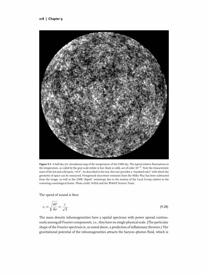
Figure 9.4 shows a map of these temperature fluctuations. The extreme isotropy of theappearance of the Universe at z ∼ 1000 is an overwhelming justification of the assumptionof homogeneity and isotropy inherent to the cosmological principle. However, this extremeisotropy raises the questions of why and how the Universe can appear so isotropic. Atthe time of recombination, the horizon size—the size of a region in space across whichlight can propagate since the Big Bang (see chapter 8, Problems 1–3)—corresponded toa physical region that subtends only about 2◦ on the sky today. Thus, different regionsseparated by more than ∼2◦ could not have been in causal contact by trec, and thereforeit is surprising that they would have the same temperature to within 10−5. CMB photonsfrom opposite directions on the sky have presumably never been in causal contact untilnow, yet they have almost exactly the same temperature.

The currently favored explanation for this “horizon problem” is that, very early during theevolution of the Universe, in the first small fraction of a second, there was an epoch of infla-tion. During that epoch, a vacuum energy density with negative pressure caused an expo-nential expansion of the scale factor, much like the second acceleration epoch that, appar-ently, we are in today. The inflationary expansion led causally connected regions to expandbeyond the size of the horizon at that time. All the different parts of the microwave sky wesee today were, in fact, part of a small, causally connected region before inflation. The causeand details of inflation are still a matter of debate, but most versions of the theory predictthat, today, space is almost exactly flat (i.e., �m + �� is very close to 1). We will see now thatthis prediction is strongly confirmed by the observed characteristics of the anisotropies.

The temperature anisotropies in the CMB arise through a number of processes, butat their root are small-amplitude inhomogeneities in the nearly uniform cosmic massdistribution. These inhomogeneities are set up at the end of the inflationary era, and theircharacteristics are yet another prediction of inflation theories. Most of the mass densityat that time, as now, is in a nonbaryonic, pressureless, dark matter. Mixed with the darkmatter, and sharing the same inhomegeneity pattern, is a relativistic gas of baryons andradiation. Thephoton–baryongas thereforehas anequationof state that iswell describedby

P = 13ρc2. (9.27)

218 | Chapter 9

Figure 9.4 A half-sky (2π steradians) map of the temperature of the CMB sky. The typical relative fluctuations inthe temperature, as coded by the gray scale (white is hot, black is cold), are of order 10−5. Note the characteristicsizes of the hot and cold spots, ≈0.4◦. As described in the text, this size provides a “standard ruler” with which thegeometry of space can be measured. Foreground microwave emission from the Milky Way has been subtractedfrom the image, as well as the CMB “dipole” anisotropy due to the motion of the Local Group relative to thecomoving cosmological frame. Photo credit: NASA and the WMAP Science Team.

The speed of sound is then

cs =√

dP

dρ= c√

3. (9.28)

The mass density inhomogeneities have a spatial spectrum with power spread continu-ously among all Fourier components, i.e., they have no single physical scale. (The particularshape of the Fourier spectrum is, as noted above, a prediction of inflationary theories.) Thegravitational potential of the inhomogeneities attracts the baryon–photon fluid, which is


compressed in the denser regions and more tenuous in the underdense regions. However,the pressure of the fluid opposes the compression, and causes an expansion that stops onlyafter the density has “overshot” the equilibrium density and the gas in the originally over-dense region has become underdense. Thus, periodic expansion and contraction of thevarious fluid regions ensues. This means that “standing” sound waves of all wavelengthsrepresented in the spatial Fourier spectrum of the density inhomogeneities are formed inthe photon–baryon gas.6 Their periods τ and wavelengths λ are related by

τ = λ

cs. (9.29)

When the Universe emerges from the inflationary era, at an age of a small fraction of asecond, these acoustic oscillations are stationary and therefore they begin everywhere inphase. Consider now an overdense or underdense region. One of the Fourier modes thatcomposes the region, and the fluid oscillations that it produces, has a wavelength thatcorresponds to a half-period of trec,

λ = 2cstrec = 2ctrec√3

, (9.30)

where trec is the cosmic time when recombination occurs. At trec, the baryon–photon fluidin this particular mode will have executed one-half of a full density oscillation, and willhave just reached its maximal rarefaction or compression, where it will be colder or hotter,respectively, than the mean. At that time, however, the baryons and photons decouple,and the imprint of the cool (rarified) and hot (compressed) regions of the mode is frozenonto the CMB radiation field, and appears in the form of spots on the CMB sky withtemperatures that are lower or higher than the mean. Similarly, higher modes that havehad just enough time, between t = 0 and t = trec, to undergo one full compression andone full rarefaction, or two compressions and a rarefaction, etc., will also be at their hottestor coldest at time trec. The CMB sky is therefore expected to display spots having particularsizes. Stated differently, the fluctutation power spectrum of the CMB sky should havediscrete peaks at these favored spatial scales.

In reality, the picture is complicated by the fact that several processes, other than adia-batic compression, affect the gas temperature observed from each point. However, all theseeffects can be calculated accurately, and a prediction of the power spectrum can be madefor a particular cosmological model. It turns out that measurement of the angular scalesat the positions of the acoustic peaks in the power spectrum, and their relative heights,can determine most of the parameters describing a cosmological model. Let us see howthis works for one example—the angular scale of the first acoustic peak as a measure ofthe global curvature of space.

As seen in Eq. 9.30, the physical scale of the first acoustic peak is the sound-crossing

horizon at the time of recombination. It therefore provides an excellent “standard ruler” at

6 The waves that are formed are not, strictly speaking, standing waves, since they do not obey boundaryconditions. They do resemble standing waves in the sense that a given Fourier component varies in phase at alllocations. However, the superposition of all these waves is not a standing wave pattern, and does not have fixednodes.

220 | Chapter 9

Figure 9.5 The angular diameter of the sound-crossing horizon (measurable fromthe size of the hot and cold spots in temperature anisotropy maps of the microwavesky), as it appears to observers in different space geometries. In a k = 0 universe(“flat” space), the spots subtend on the sky an angle θ given by Euclidean geometry.In a k = +1 Universe, the angles of a triangle with sides along geodesics sum to>180◦. Since light follows a geodesic path, the converging light rays from the twosides of a CMB “spot” will bend, as shown, along their path, and θ will appear largerthan in the k = 0 case. For negative space curvature, the angles in the triangle sumto <180◦, and θ is smaller than in the flat case.

a known distance. The angle subtended on the sky by this standard ruler (i.e., the angle ofthe first peak) can be predicted for every geometry (i.e., curvature) of space. Comparisonto the observed angle thus reveals directly what that geometry is (see Fig. 9.5).

Consider, for example, a flat (k = 0) cosmology with no cosmological constant. We wishto calculate the angular size on the sky, as it appears today, of a region of physical size(Eq. 9.30)

Ds = 2ctrec√3

= 2 × 400, 000 ly√3

= 140 kpc, (9.31)

from which light was emitted at time trec. Between recombination and the present time,the Universal expansion is matter-dominated, with R ∝ t2/3 for this model, i.e.,

R

R0=(

t

t0

)2/3

= 1

1 + z, (9.32)

and hence we can also write Ds as

Ds = 2ct0√3

(1 + zrec)−3/2. (9.33)

The angle subtended by the region equals its size, divided by its distance to us at the time

of emission (since that is when the angle between rays emanating from two sides of theregion was set). As we are concerned with observed angles, the type of distance we areinterested in is the distance that, when squared and multiplied by 4π , will give the areaof the sphere centered on us and passing through the said region. If the comoving radial


coordinate of the surface of last scattering is r , the required distance is currently just r × R0,and is called the proper-motion distance. (For k = 0, the proper distance and the propermotion distance are the same, as can be seen from Eq. 8.10.) The proper motion distancecan again be found by solving for the null geodesic in the FRW metric (see Eq. 9.2),

∫ t0

t rec

cdt

R(t)=∫ r

0

dr√1 − kr2

. (9.34)

Setting k = 0, and substituting

R(t) = R0

(t

t0

)2/3

, (9.35)

we integrate and find

rR0 = 3ct0

[1 −

(trec

t0

)1/3]

= 3ct0[1 − (1 + zrec)−1/2]. (9.36)

However, at the time of emission, the scale factor of the Universe was 1 + z times smaller.The so-called angular-diameter distance to the last scattering surface is therefore

DA = rR0

1 + z= 3ct0[(1 + zrec)−1 − (1 + zrec)−3/2]. (9.37)

The angular size of the sound-crossing horizon at the recombination era in a k = 0cosmology is thus expected to be

θ = Ds

DA= 2ct0(1 + zrec)−3/2

3√

3ct0[(1 + zrec)−1 − (1 + zrec)−3/2]= 2

3√

3[(1 + zrec)1/2 − 1] . (9.38)

Since recombination occurs at Trec ≈ 3000 K, and the current CMB temperature is 2.7 K,zrec ≈ 1100, and

θ ≈ 0.012 radian = 0.7◦. (9.39)

For this particular cosmological model (k = 0, �� = 0), this will be the angular scale ofthe first acoustic peak in the Fourier spectrum of the CMB fluctuations. The hot and cold“spots” in CMB sky maps will correspond to half a wavelength, i.e., will have half thisangular size, or somewhat smaller than the diameter of the full Moon (half a degree).In a negatively curved geometry, where the angles of a triangle add up to less than 180◦,the angle subtended by the standard ruler of length 2cstrec will be smaller than in a flatgeometry. In a positively curved Universe, this angle will appear larger than in the flat case.

Recent measurements of the CMB fluctuation power spectrum provide spectacularconfirmation of the expected acoustic peaks (see Fig. 9.6). When compared to more

222 | Chapter 9

Figure 9.6 Observed angular power spectrum of temperature fluctuations in the CMB.The top axis shows the angular scales corresponding to the spherical harmonic multipoleson the bottom axis. The curve is based on a detailed calculation of the fluctuation spectrumusing values for the various cosmological parameters that give the best fit to the data. Notethe clear detection of acoustic peaks, with the first peak on a scale θ ≈ 0.8◦, indicating aflat space geometry. Data credits: NASA/WMAP, CBI, and ACBAR collaborations.

sophisticated calculations that account for all the known effects that can influence the tem-perature anisotropies, the location of the first peak indicates a nearly flat space geometry,with

�m + �� = 1.02 ± 0.02. (9.40)

Note that a region with the diameter of the sound-crossing horizon has, between recombi-nation and the present, expanded by 1 + zrec = 1100, and hence encompasses today (i.e.,has a comoving diameter) 140 kpc × 1100 = 150 Mpc. Thus, the CMB hot and cold spotscorrespond to regions that, today, are quite large.

Among a number of other cosmological parameters that are determined by analysis ofthe observed CMB anisotropy power spectrum are

�m ≈ 0.3, (9.41)

which together with Eq. 9.40 confirms the result found from the Hubble diagram of type Iasupernovae, that the dynamics of the Universe are currently dominated by a cosmologicalconstant with

�� ≈ 0.7. (9.42)

If one assumes that the Universe is exactly flat, then the CMB results also give a preciseage of the Universe

t0 = 13.7 ± 0.2 Gyr, (9.43)


and a density in baryons

�B = 0.044 ± 0.004. (9.44)

The mere existence of acoustic peaks in the power spectrum means that density pertur-bations existed long before the time of recombination, i.e., they were primordial, and thatthey had wavelengths much longer than the horizon size at the time they were set up.Inflation is the only theory that currently predicts, based on causal physics, the existenceof primordial, superhorizon-size, perturbations. The observation of the acoustic peaks cantherefore be considered as another successful prediction of inflation.

The large density inhomogeneities we see today—stars, galaxies, and clusters—formedfrom the growth of the initial small fluctuations, the traces of which are observed in theCMB. The gravitational pull of small density enhancements attracted additional mass, atthe expense of neighboring underdense regions. The growing clumps of dense mattermerged with other clumps to form larger clumps. This growth of structure by means ofgravitational instability operated at first only on the nonbaryonic dark-matter fluctuations,but not the baryons, which were supported against gravitational collapse by radiationpressure. Once the expansion of the Universe became matter-dominated, the dark-matterdensity perturbations could begin to grow at a significant rate. Finally, after recombination,the baryons became decoupled from the photons and their supporting radiation pressure,and the perturbations in the baryon density field could also begin to grow. The detailsand specific path according to which structure formation proceeds is still the subject ofactive research. Nevertheless, it is clear that, once the first massive stars formed (endingthe period sometimes called the Dark Ages), they reionized most of the gas in the Uni-verse. Based again on analysis of the CMB, current evidence is that this occurred duringsome redshift in the range between ∼6 and 20, when the Universe was 150–750 Myrold.

By this time, the mean matter density was low enough that the newly liberated electronswere a negligible source of opacity, and hence the Universe remained transparent (seeProblem 2). Direct evidence that most of the gas in the Universe is, at z ∼ 6 and below,almost completely ionized, comes from the fact that objects at those redshifts are visibleat UV wavelengths shorter than Lyman-α; even a tiny number of neutral hydrogen atomsalong the line of sight would suffice to completely absorb such UV radiation, due to thevery large cross section for absorption from the ground state of hydrogen (often calledresonant absorption). Most of the gas in the intergalactic medium (which is the main currentrepository of baryons) remains in a low-density, hot, ionized phase. The density of thisgas is low enough that the recombination time is longer than the age of the Universe, andhence the atoms will never recombine.

9.4 Nucleosynthesis of the Light Elements

Looking back in time to even earlier epochs than those discussed so far, the temperature ofthe Universe must have been high enough that electrons, protons, positrons, and neutrons

224 | Chapter 9

were in thermodynamical equilibrium. Since the rest-mass energy difference between aneutron and a proton is

(mn − mp)c2 = 1.3 MeV, (9.45)

at a time t 1 s, when the temperature was T � 1 MeV (1010 K), the reactions

e− + p + 0.8 MeV � νe + n (9.46)

and

νe + p + 1.8 MeV � e+ + n (9.47)

could easily proceed in both directions. The ratio between neutrons and protons as afunction of temperature can be obtained from statistical mechanics considerations via theSaha equation. For the case at hand, it takes the form

Nn

Np=(

mn

mp

)3/2

exp[− (mn − mp)c2

kT

]. (9.48)

When T � 1 MeV, the ratio is obviously very close to 1. As the temperature decreases, theratio also decreases, and protons outnumber the heavier neutrons. This decrease in theratio could continue indefinitely, but when T < 0.8 MeV, the mean time for reaction 9.46becomes longer than the age of the Universe at that epoch, t = 2 s. The reaction time canbe calculated from knowledge of the densities of the different particles, the temperature,and the cross section, as outlined for stellar nuclear reactions in Eqs. 3.123–3.127. The longreaction timescale means that the neutrons and protons, which are converted from one tothe other via this reaction are no longer in thermodynamic equilibrium.7 This time is calledneutron freezeout, since neutrons can no longer be created. The neutron-to-proton ratiotherefore “freezes” at a value of exp(−1.3/0.8) = 0.20. In the following few minutes, mostof the neutrons become integrated into helium nuclei. This occurs through the reactions

n + p → d + γ (9.49)

p + d →3 He + γ (9.50)

d + d →3 He + n (9.51)

n +3He →4 He + γ (9.52)

d +3He →4 He + p. (9.53)

Some of the neutrons undergo beta decay into a proton and an electron before making itinto a helium nucleus (the mean lifetime of a free neutron is about 15 min), and a smallfraction is integrated into other elements. Numerical computation of the results of all theparallel nuclear reactions that occur as the Universe expands, and as the density and thetemperature decrease, shows that, in the end, the ratio between neutrons inside 4He andprotons is about 1/7. Thus, for every 2 neutrons there are 14 protons. Since every 4He

7 At about the same time, neutrinos also decouple (i.e., cease to be in thermal equilibrium with the rest of thematter and the radiation), and the cosmic neutrino background is formed; see Problem 9.


nucleus has 2 neutrons and 2 protons, there are 12 free protons for every 4He nucleus, orthe ratio of helium to hydrogen atoms is 1/12. The mass fraction of 4He will then be

Y4 = 4N(4He)

N(H) + 4N(4He)= 4 1

12

1 + 4 112

= 1

4. (9.54)

A central prediction of Big Bang cosmology is therefore that a quarter of the mass inbaryons was synthesized into helium in the first few minutes.

Measurements of helium abundance in many different astronomical settings (stars,H II regions, planetary nebulae) indeed reveal a helium mass abundance that is consistentwith this prediction. This large amount of helium could not plausibly have been producedin stars. On the other hand, the fact that the helium abundance is nowhere observed tobe lower than ≈0.25 is evidence for the unavoidability of primordial helium synthesis, atthis level, among all baryons during the first few minutes.

Apart from 4He, trace amounts of the following elements are produced during the firstminutes: deuterium (10−5), 3He (10−5), 7Li (10−9), 7Be (10−9), and almost nothing else.The precise abundances of these elements depend on the baryon density, nB, at the time ofnucleosynthesis. As we have seen (Eqs. 8.40, 9.13), the radiation energy density declinesas R−4, but the temperature appearing in the Planck spectrum also declines as T ∝ 1/R,both before and after recombination. Since the energy of the photons scales with kT , thephoton number density declines as R−3. Because baryons are conserved, their densityalso declines as R−3 when the Universe expands, and therefore the baryon-to-photon ratio(Eq. 9.25), η ≈ 5 × 10−10, does not change with time. Since we know the CMB photondensity today, nγ , measurements of the abundances of the light elements in astronomicalsystems that are believed to be pristine, i.e., that have undergone minimal additionalprocessing in stars (which can also produce or destroy these elements) lead to an estimateof the baryon density today. In units of the critical closure density, ρc ,

�B = nBmp

ρc= η nγ mp

ρc. (9.55)

The baryon density based on these measurements is

0.01 < �B < 0.05. (9.56)

As already mentioned, a completely independent estimate of �B comes from analyzingthe fluctuation spectrum of CMB anisotropies. The relative amplitudes of the acousticpeaks in the spectrum depend on the baryon density and hence constrain it to

�B = 0.044 ± 0.004, (9.57)

in excellent agreement with the value based on element abundances. Note that both of thesemeasurements tell us that, even though the mass density of the Universe is a good fractionof the closure value (�m ≈ 0.3), only a about a tenth of this mass is in baryons, while the restmust be in a dark matter component of unknown nature. Furthermore, less than 1/10 ofthe baryons are in stars inside galaxies. The bulk of the baryons are apparently in a tenuous,hot, and ionized intergalactic gas—the large reservoir of raw material out of which galaxiesformed. A small fraction of this gas is neutral, and can be observed by the absorption itproduces in the spectra of distant quasars. This is discussed briefly in section 9.5.

226 | Chapter 9

Table 9.1 History and Parameters of the Universe

Curvature: �m + �� = 1.02 ± 0.02

Mass density: �m,0 ≈ 0.3, consisting of

�B,0 = 0.044 ± 0.004 in baryons, and

�DM,0 ≈ 0.25 in dark matter

Dark energy: �� ≈ 0.7

Redshift Temperature

Time z T (K) Event

∼10−34 s ∼1027 ∼1027 Inflation ends, �m + �� → 1, causally connected

regions have expanded exponentially, initial fluctuation

spectrum determined.

2 s 4 × 109 1010 Neutron freezeout, no more neutrons formed.

3 min 4 × 108 109 Primordial nucleosynthesis over—light element

abundances set.

65,000 yr 3500 104 Radiation domination → mass domination,

R ∼ t1/2 → R ∼ t2/3, dark-matter structures start

growing at a significant rate.

400,000 yr 1100 3000 Hydrogen atoms recombine, matter and radiation

decouple, Universe becomes transparent to radiation

of wavelengths longer than Lyα, CMB fluctuation

pattern frozen in space, baryon perturbations start

growing.

∼108–109 yr ∼6–20 ∼20–60 First stars form and reionize the Universe, ending

the Dark Ages. The Universe becomes transparent also

to radiation with wavelengths shorter than Lyα.

∼6 Gyr ∼1 ∼5 Transition from deceleration to acceleration under

the influence of dark energy.

14 Gyr 0 2.725 ± 0.002 Today.

Table 9.1 summarizes the current view of the cosmological parameters and the historyof the Universe.

9.5 Quasars and Other Distant Sources as Cosmological Probes

Quasars, which we discussed in section 6.3, are supermassive black holes accreting at ratesthat produce near-Eddington luminosities of 101–104L∗. Their large luminosities make


Figure 9.7 A high-resolution spectrum of a quasar at redshift z = 3.18, with the Lyman α

emission line redshifted to 5080 Å. Note the Lyman-α forest of absorption lines starting fromthe peak of the emission line, and continuing in the blue (left) direction. These lines are dueto Lyman-α absorption by neutral hydrogen atoms in gas clouds that are along the line ofsight to the quasar, and hence at lower redshifts than the quasar. The few absorption linesto the red of the Lyman-α emission line peak are due to heavier elements and are associatedwith the system that produces the strong damped Lyman-α absorption observed at ≈4650 Å.Data credit: W. Sargent and L. Lu, based on observations with the HIRES spectrograph at theW. M. Keck Observatory.

quasars easily visible to large cosmological distances, and allow probing the assembly andaccretion history of the central black holes of galaxies. As noted in chapter 6, luminousquasars are rare objects at present, and apparently most central black holes in nearbygalaxies are accreting at low or moderate rates, compared to the rates that would producea luminosity of LE . However, quasars were much more common in the past, and theircomoving space density reached a peak at an epoch corresponding to redshift z ∼ 2 (i.e.,about 10 Gyr ago). There is likely a connection between the growth and development ofgalaxies and of their central black holes, and quasar evolution may hold clues to decipheringthis connection (see Problem 11). The most distant quasars currently known are at red-shifts beyond z = 6, and are therefore observed less than 1 Gyr after the Big Bang. Modelsof structure formation suggest that the first galaxies began to assemble at about thattime.

Since quasars are so luminous, they are also useful cosmological tools, in that theycan serve as bright and distant sources of light for studying the contents of the Universebetween the quasars and us. One such application is the study of quasar absorption lines.The light from all distant quasars is seen to be partially absorbed by numerous clouds ofgas along the line of sight. A small fraction (∼10−4) of the hydrogen in these clouds isneutral, and is manifest as a “forest” of redshifted absorption lines (mostly Lyman-α) in thespectrum of each quasar (see Fig. 9.7). Each absorption line is at the wavelength of Lyman-α redshifted according to the distance of the particular absorbing cloud. The absorptionlines are therefore distributed in wavelength between the rest wavelength of Lyα at 1216 Åand the observed, redshifted Lyα wavelength of the quasar (say, (1 + z)1216 Å = 3648 Å,for a z = 2 quasar).

228 | Chapter 9

Apart from the hydrogen Lyman-α lines, additional absorption lines are detected.Absorption lines produced by heavier elements in the same clouds allow estimating the“metallicities” of these clouds, and reveal very low element abundances, i.e., the gas inthe clouds has undergone little enrichment by stellar processes. It is in such clouds thatthe abundance of primordial deuterium can be measured and compared to Big Bangnucleosynthesis predictions (see section 9.4). The Lyman-α clouds are one component (arelatively cool one, with T ∼ 104 K) of the intergalactic medium. Most of the intergalacticgas, however, is apparently in a hotter T ∼ 105−6 K, more tenuous, component. Estimatesof the total mass density of intergalactic gas find that the bulk of the baryons in the Universeis contained in this hot component, while less than about 10% of the baryons are in galaxiesin the form of stars and cold gas.

Another application in which quasars serve as distant light sources for probing theintervening matter distribution is in cases where galaxies or galaxy clusters gravitationallylens quasars that are projected behind them, splitting them into multiple images.8 Sincethe lensing objects in such cases are at cosmological distances (∼1 Gpc), and the lensingmasses are of order 1011M�, the Einstein angle (Eq. 6.25), which gives the characteristicangular scale of the split images, is of order 1 arcsecond, i.e., resolved by telescopes atmost wavelength bands, from radio through X-rays (see Fig. 9.8). Modeling of individualsystems can reveal the shapes and forms of the mass distributions, both the dark and theluminous. The statistics of lensed quasars (e.g., measurement of the fraction of quasarsthat are multiply imaged by intervening galaxies) can provide information on the propertiesof the galaxy population and its evolution with cosmic time (see chapter 6, Problem 6). Notonly quasars serve as background light sources for galaxy lenses—there are many knowncases of galaxies that lens other galaxies that lie behind them (also shown in Fig. 9.8), andsuch systems can be used for the same applications.

In known systems in which a galaxy or a galaxy cluster operate as a powerful gravitationallens, one can turn the problem around and use the lens as a “natural telescope.” Once theproperties of the lens have been derived, based on the positions and relative magnificationsof the lensed images of the bright background quasar or galaxy, one can search otherregions of the lens that are then expected to produce high magnification for lensed imagesof additional background objects. This method of “searching under the magnifying glass”has been used to find and study galaxies with luminosities as low as 0.01L∗ out to redshiftsz ∼ 6, aided by the natural magnification of galaxy clusters.

With these and other techniques, it is hoped that a detailed and consistent picture ofcosmic history will eventually emerge. Such an understanding would include the natureof dark matter and dark energy, their interplay with baryons and with supermassive blackholes in the formation of the first stars and galaxies, the element enrichment of the inter-stellar and the intergalactic medium by generations of evolved stars and supernovae, andthe evolution of galaxies and their constituents, all the way to the world as we see it today.

8 Since galaxy mass distributions are generally not spherically symmetric, when they act as gravitational lensesthey can split background sources into multiple images, rather than just deforming the sources into rings orsplitting them into double images, as is the case for point masses and spherically symmetric masses.


Figure 9.8 Top two rows: Examples of quasars that are gravitationally lensed into multiple images by interveninggalaxies. In each case, the lens galaxy, at a redshift of z ≈ 0.04–0.7, is the extended central object, and the twoor four sources straddling it are the multiply lensed images of a background quasar, at z ≈ 1.7–3.6. Panelsare 5 arcseconds on a side. Some image processing has been applied, to permit seeing clearly both the bright,point-like, quasar images and the faint, extended lens galaxies. Bottom row: Examples of foreground galaxies thatlens background galaxies into partial or full Einstein rings. In the cases shown, the foreground galaxies are at z ≈0.2–0.4 and the background galaxies are at z ≈ 0.5–1. Photo credits: The CASTLES gravitational lens database,C. Kochanek et al.; NASA, ESA, J. Blakeslee and H. Ford,; and NASA, ESA, A. Bolton, S. Burles, L. Koopmans,T. Treu, and L. Moustakas.

Problems

1. In an accelerating or decelerating Universe, the redshift z of a particular source willslowly change over time t0, as measured by an observer.a. Show that the rate of change is

dz

dt0= H0(1 + z) − H(z),

where H(z) ≡ Re/Re is the Hubble parameter at the time of emission.

230 | Chapter 9

Hint: Differentiate the definition of redshift, 1 + z ≡ R0/Re, with respect to t0. Usethe chain rule to deal with expressions such as dRe/dt0.

b. Show that, for a k = 0 universe with no cosmological constant,H(z) = H0(1 + z)3/2.For thismodel, and assumingH0 = 70 kms−1Mpc−1, evaluate the change in redshiftover 10 years, for a source at z = 1, and the corresponding change in “recessionvelocity”.Answers: �z = −5.9 × 10−10, � = −18 cm s−1.

2. At a redshift z = 1100, atoms were formed, the opacity of the Universe to radiation viaelectron scattering disappeared, and the cosmic microwave background was formed.Imagine aworld inwhich atomscannot form. Even thoughsuchauniverse, by definition,will remain ionized forever, after enough time the density will decline sufficiently tomake the universe transparent nonetheless. Find the redshift at which this would havehappened, for a k = 0 universe with no cosmological constant. Assume an all-hydrogencomposition, �B = 0.04, and H0 = 70 km s−1Mpc−1. Note that this calculation is notso farfetched. Following recombination to atoms at z = 1100, most of the gas in theUniverse was reionized sometime between z = 6 and z = 20 (probably by the firstmassive stars that formed), and has remained ionized to this day. Despite this fact, theopacity due to electron scattering is very low, and our view is virtually unhindered outto high redshifts.Hint: A “Universe transparent to electron scattering” can be defined in several ways.One definition is to require that the rate at which a photon is scattered by electrons,neσTc, is lower than the expansion rate of the Universe at that time, H (or, in otherwords, the time between two scatters is longer than the age of the Universe at thattime). To follow this path (which is called decoupling between the photons and thehypothetical free electrons), express the electron density ne at redshift z, by startingwith the current baryon number density, �Bρcr,0/mp, expressing ρcr,0 by means of H0,and increasing the density in the past as (1 + z)3. Similarly, write H in terms of H0 and(1 + z) (recall that 1 + z = R0/R, and in this cosmology, R ∝ t2/3 and H ∝ t−1). Showthat decoupling would have occurred at

1 + z =(

8πGmp

3�BH0σT c

)2/3

,

and calculate the value of this redshift. Alternatively, we can find the redshift of the “lastscattering surface” from which a typical photon would have reached us without furtherscatters. The number of scatters on electrons that a photon undergoes as it travels fromredshift z to redshift zero is∫ l(z)

0ne(z)σT dl.

Express ne, as above, in terms of �B, H0, and 1 + z, replace dl with c(dt/dz)dz, usingagain R ∝ t2/3 to write dt/dz in terms ofH0 and 1 + z. Equate the integral to 1, performthe integration, show that the last scattering redshift would be


1 + z =(

4πGmp

�BH0σT c

)2/3

,

and evaluate it.Answers: z = 65; z = 85.

3. Show that the angular-diameter distance for a flat space (k = 0; Eq. 9.37) out toredshift z,

DA = 3ct0[(1 + z)−1 − (1 + z)−3/2],has a maximum with respect to redshift z, and find that redshift. The angular size onthe sky of an object with physical size d is θ = d/DA. What is the implication of themaximum of DA for the appearance of objects at redshifts beyond the one you found?Note that this peculiar behavior is simply the result of light travel time out to differentdistances in an expanding universe; an object at high redshift may have been closer tous at the time of emission than an object of the same size at a lower redshift, despitethe fact that the high-redshift object is currently more distant.

4. a. Consider the energy flux of photons from a source with bolometric luminosity L andwith proper-motion distance rR0. The photons will be spread over an area 4π (rR0)2.Explain why the observed photon flux will be

f = L

4π (rR0)2(1 + z)2.

Hint: Consider the effects of redshift on the photon energy and cosmological timedilation on the photon arrival rate. This relation is used to define the luminositydistance, DL = rR0(1 + z).

b. Find DL(z) for a k = 0 universe without a cosmological constant. Plot, for this worldmodel, the Hubble diagram, i.e., the flux vs. z, from an object of constant luminosity.

5. Show that in a Euclidean, nonexpanding, universe, the surface brightness of an object,i.e., its observed flux per unit solid angle (e.g., per arcsecond squared), does not changewith distance. Then, show that in an expanding FRW universe, the ratio between theluminosity distance (see Problem 4) and the angular-diameter distance to an objectis always (1 + z)2. Use this to prove that, in the latter universe, surface brightnessdims with increasing redshift as (1 + z)−4. This effect makes extended objects, such asgalaxies, increasingly difficult to detect at high z.

6. Anobject at proper-motion distance rR0 splits into twohalves. Each piecemoves relativeto the other, perpendicular to our line of sight, at a constant, nonrelativistic, velocity .What is the the angular rate of separation, or “proper motion” between the two objects(i.e., the change of angle per unit time)?Hint: Recall that we are measuring an angle, and so require the angular-diameter dis-tance, but we are alsomeasuring a rate, which is affected by cosmological time dilation.You can now see why rR0 is called the proper-motion distance.

232 | Chapter 9

7. Use the first Friedmann equation with a nonzero cosmological constant (Eq. 8.95) toshow that, in a flat, matter-dominated Universe, the proper-motion distance is

rR0 =∫

cdz

H0

√�m,0(1 + z)3 + ��,0

.

Use a computer to evaluate this integral numerically with �m,0 = 0.3 and ��,0 = 0.7,for values of z between 0 and 2. Plot the Hubble diagram, i.e., flux vs. z, from anobject of constant luminosity, in this case, and compare to the curve describing k = 0,�m = 1 (Problem 4). You can now see how the Hubble diagram of type Ia supernovaecan distinguish among cosmological models.Hint: Set k = 0 in Eq. 8.95, replace ρ by ρoR3

0/R3 (matter domination), divide both

sides by H20, and substitute the dimensionless parameters �m,0 and ��,0. Change

variables from R to z with the transformation 1 + z = R0/R, and separate the variablesz and t. Finally, use the FRW metric for k = 0: cdt = Rdr = R0/(1 + z)dr, and hencerR0 = ∫

(1 + z)cdt, to obtain the desired result.

8. Emission lines of hydrogen Hβ (n = 4 → 2, λrest = 4861 Å) are observed in the spec-trum of a spiral galaxy at redshift z = 0.9. The galaxy disk is inclined by 45◦ to the line ofsight.a. The Hβ wavelength of lines from one side of the galaxy are shifted to the blue by 5 Å

relative to the emission line from the center of the galaxy, and to the red by 5 Å onthe other side. What is the galaxy’s rotation speed?

b. Analysis of the emission from the active nucleus of the galaxy reveals a total redshiftof z = 1. If the additional redshift is gravitational, the result of the proximity of theemitting material to a black hole, find this proximity, in Schwarzschild radii.Hint: Note that all redshift and blueshift effects are multiplicative, e.g., (1+ ztotal) =(1 + zcosmological)(1 + sini/c), or (1 + ztotal) = (1 + zcosmological)(1 + zgravitational).

c. Find the age of the Universe at z = 0.9, assuming an expansion factor R ∝ t2/3, anda current age t0 = 13.7 Gyr. What is the “lookback time” to the galaxy?Answers: 230 km s−1; 11rs; lookback time 8.5 Gyr.

9. At some point back in cosmic time, the Universe was dense enough to be opaqueto neutrinos. Then, as the Universe expanded, the density decreased until neutrinoscould stream freely. A cosmic neutrino background (which is undetected to date) musthave formed when this decoupling between neutrinos and normal matter occurred, inanalogy to the CMB that results from the electron–photon decoupling at the time ofhydrogen recombination. Find the temperature at which neutrino decoupling occurred.Assume in your calculation that decoupling occurs during the radiation-dominatedera, photons pose the main targets for the neutrinos, neutrino interactions have anenergy-dependent cross section

σνγ = 10−43 cm2

(Eν

1 MeV

)2

,

and the neutrinos are relativistic. Use a k = 0, �� = 0 cosmology.


Hint: Proceed by the first method of Problem 2, i.e., by requiring nσ = H. Representthe “target” density, n, by aT 4/kT, where a is the Stefan-Boltzmann (or “radiation”)constant. Use σνγ for the cross section σ , but approximating Eν as kT. The velocityequals c, because the neutrinos and the target particles are relativistic. To representH,use the first Friedmann equation,

H2 = 8πGρrad

3c2,

with ρrad = aT 4.Answer: kT = 1 MeV.

10. It has been found recently that every galactic bulge harbors a central black hole with amass ∼0.001 of the bulge mass. The mean space density of bulges having 1010M� isabout 10−2 Mpc−3.a. Find the mean density of mass in black holes, in units ofM� Mpc−3.b. If all these black holes were shining at their Eddington luminosities, what would

be the luminosity density, in units of L� Mpc−3? How does this compare to theluminosity density from stars?

c. Theobserved luminosity density of quasars andactive galaxies, averagedover cosmictime, is actually 100 times less than calculated in (b). If all central black holes havegone through an active phase, what does this imply for the total length of time thata black hole is “active"?

11. The most distant quasars currently known are at redshift z ∼ 6, and have luminositiesL ∼ 1047 erg s−1.a. Find a lower limit to themass of the black hole powering such a quasar, by assuming

it is radiating at the Eddington limit.b. Find the age of the Universe at z = 6, assuming an expansion R ∝ t2/3 and a current

age t0 = 13.7 Gyr.c. Equate the Eddington luminosity LE(M) as a function of massM to the luminosity of

an accretion disk around a black hole with a mass-to-energy conversion efficiency of0.06. This will give you a simple differential equation forM(t), describing the growthof a black hole. Solve the equation (be careful with units).

d. Suppose a black hole beginswith a “seed”mass of 10M� and shines at the Eddingtonluminosity continuously. How long will it take the black hole to reach themass foundin (a)? By comparing to the result of (b), what is the minimum redshift at whichaccretion must begin?Answers: ∼109M�; t(z = 6) = 740 Myr; M = Mseedexp(t/τ ), with τ = 26 Myr;480 Myr, z(t = 260 Myr) = 13.

Documents

Chapter 9 - PRINCETON University Press