Embed Size (px)
Citation preview
M O N I T O R I N G O F S P E C I E S A N D H A B I T A T S
4
Monitoring of species and habitats
CHAPTER A . I .
Anne Schmidt & Chris van Swaay
5M O N I T O R I N G O F S P E C I E S A N D H A B I T A T S
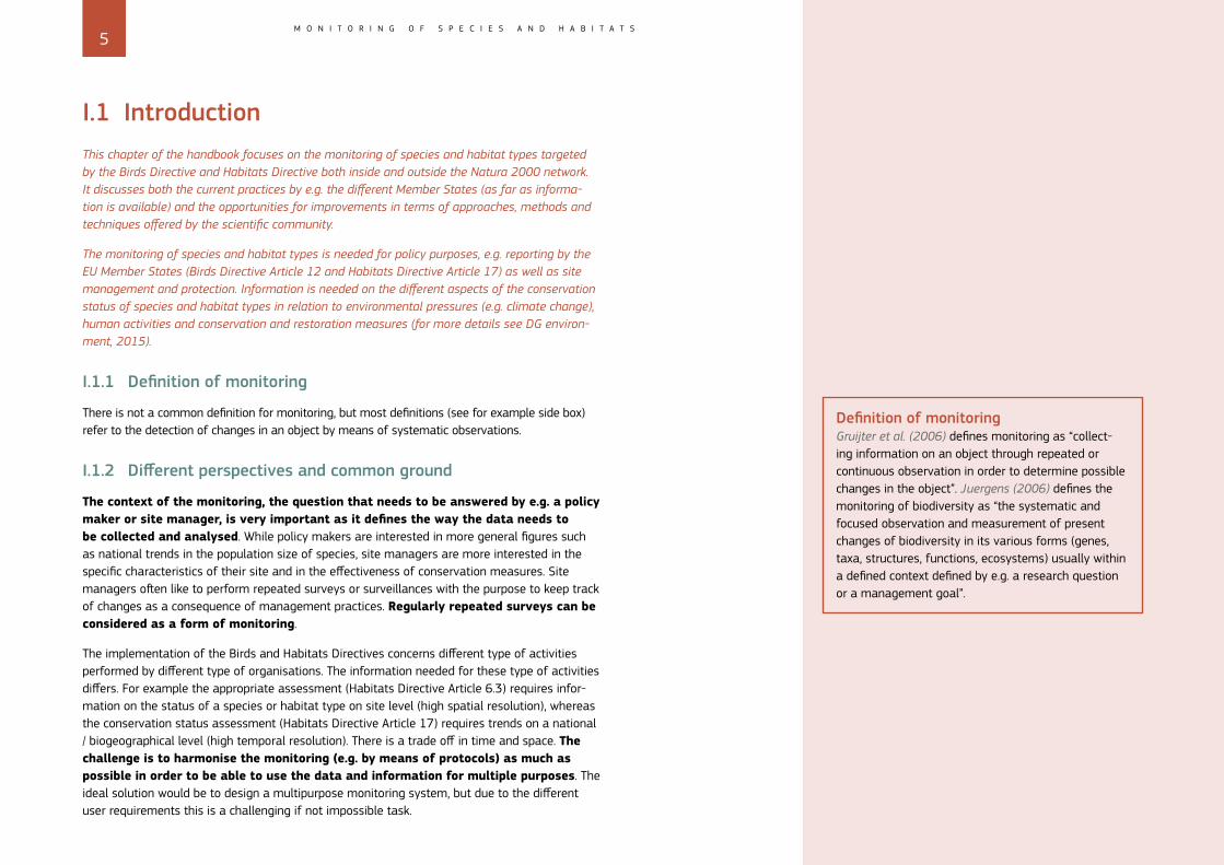
I.1 IntroductionThis chapter of the handbook focuses on the monitoring of species and habitat types targeted by the Birds Directive and Habitats Directive both inside and outside the Natura 2000 network. It discusses both the current practices by e.g. the different Member States (as far as informa-tion is available) and the opportunities for improvements in terms of approaches, methods and techniques offered by the scientific community.
The monitoring of species and habitat types is needed for policy purposes, e.g. reporting by the EU Member States (Birds Directive Article 12 and Habitats Directive Article 17) as well as site management and protection. Information is needed on the different aspects of the conservation status of species and habitat types in relation to environmental pressures (e.g. climate change), human activities and conservation and restoration measures (for more details see DG environ-ment, 2015).
I.1.1 Definition of monitoring
There is not a common definition for monitoring, but most definitions (see for example side box) refer to the detection of changes in an object by means of systematic observations.
I.1.2 Different perspectives and common ground
The context of the monitoring, the question that needs to be answered by e.g. a policy maker or site manager, is very important as it defines the way the data needs to be collected and analysed. While policy makers are interested in more general figures such as national trends in the population size of species, site managers are more interested in the specific characteristics of their site and in the effectiveness of conservation measures. Site managers often like to perform repeated surveys or surveillances with the purpose to keep track of changes as a consequence of management practices. Regularly repeated surveys can be considered as a form of monitoring.
The implementation of the Birds and Habitats Directives concerns different type of activities performed by different type of organisations. The information needed for these type of activities differs. For example the appropriate assessment (Habitats Directive Article 6.3) requires infor-mation on the status of a species or habitat type on site level (high spatial resolution), whereas the conservation status assessment (Habitats Directive Article 17) requires trends on a national / biogeographical level (high temporal resolution). There is a trade off in time and space. The challenge is to harmonise the monitoring (e.g. by means of protocols) as much as possible in order to be able to use the data and information for multiple purposes. The ideal solution would be to design a multipurpose monitoring system, but due to the different user requirements this is a challenging if not impossible task.
Definition of monitoring Gruijter et al. (2006) defines monitoring as “collect-ing information on an object through repeated or continuous observation in order to determine possible changes in the object”. Juergens (2006) defines the monitoring of biodiversity as “the systematic and focused observation and measurement of present changes of biodiversity in its various forms (genes, taxa, structures, functions, ecosystems) usually within a defined context defined by e.g. a research question or a management goal”.
6M O N I T O R I N G O F S P E C I E S A N D H A B I T A T S
GEO-BON is developing the “Essential Biodiversity Variables” (EBVs) framework (Pereira et al., 2013; Jetz et al., 2019) with the purpose of representing a minimal set of fundamental observations needed to support multi-purpose, long term biodiversity information needs at various scales (Walters and Scholes, 2017). The EBVs fall in six classes: genetic composition, species populations and ranges, species traits, community composition, ecosys-tem structure and ecosystem function. These EBVs overlap to a large extent with the different aspects of the conservation status of species (species distribution/range and population, habitat for species) and habitat types (distribution/range, area, structure and function) of the Birds and Habitats Directive.
I.1.3 Smart sampling and data analysis methods
Both regularly repeated surveys and monitoring are based on sampling. Many sam-pling-related methods and techniques are generally applicable: in space, in time and in time-space (Gruijter et al., 2006).
Different monitoring objectives require different sampling designs. That makes it difficult to de-sign a multipurpose monitoring system. Trend monitoring (e.g. the increase or decline in popula-tion size of species) requires other sampling strategies than status monitoring (e.g. the estimate of the total number of individuals). If one wants to study causal relationships, e.g. the effects of conservation measures on the status of a species, a specific sampling scheme is required such as a Before-After-Control-Impact (BACI) design.
The conservation status is a legal concept from the Habitats Directive. It describes the status of a species or habitat type targeted by the Directive and is assessed based on several conserva-tion status parameters, namely the distribution and range of the species/habitat type, the pop-ulation size of the species/the habitat area and the area and quality of the habitat for species/the structure and function of habitat type. In addition (mainly based on the trends) the future prospects of all these parameters are estimated. The conservation status in fact is based on the aggregation of the assessment of all these parameters.
In chapter I.2 existing sampling and data analysis methods are described to retrieve information on the conservation parameters of the species and habitat types.
I.1.4 Observation technologies
There are different ways to collect data on species and habitat types. The most classical way of data collection is a field survey (field observations and measurements). This is often labour intensive. Nowadays there are different techniques available for collecting data such as DNA sampling, camera traps, etc., that can be (partly) automated and might be less labour intensive.
In chapter I.3 a selection of observation technologies is described that are or might be applied to collect data on species and habitat types.
Status being the state or condition in a certain moment at time (e.g. the total number of birds at a certain location at a certain moment in time).
Trend being a change or direction (e.g. an increase in the number of birds at a certain location during a certain period).
7M O N I T O R I N G O F S P E C I E S A N D H A B I T A T S
I.1.5 Modelling techniques
Nowadays there are data modelling techniques available by means of which relevant informa-tion is retrieved from non-structured opportunistic data. These techniques and methodologies are very valuable to fill in the gaps in data and information needed for the implementation of the Birds and Habitats Directives, amongst others concerning the distribution of species and habitat types. These models can help as well to explain the occurrence and/or abundance of species and habitat types in relation to the environmental conditions including certain pressures and threats.
In chapter I.4 modelling techniques are described by means of information that can be retrieved on different conservation parameters of species and habitat types, specifically species and habitat type distribution.
I.1.6 Monitoring approaches, constraints and priorities
Different monitoring approaches are followed by the Member States depending on the availability of funding and the existence of volunteer networks.
There is a difference between the MS with regard to state funding and the involvement of skilled amateur volunteers. Where state agencies have small budgets, there are fewer skilled professionals or amateurs, and socioeconomic conditions prevent development of a culture of volunteerism (Danielsen et al., 2009). The resulting lack of knowledge about trends in species and habitats presents a serious challenge for detecting, understanding, and reversing declines in natural resource values (Danielsen et al., 2009).
Some MS build on existing monitoring programmes by adapting or extending monitoring schemes. Other MS start from scratch (based on best practices) and develop monitoring pro-grams tailored to e.g. the reporting obligations.
Priorities need to be set depending on the resources that are available (in terms of budget as well experts and/or volunteers). In order to meet the objectives of the directives the most logic choice is to focus on those species and habitat types that are most threatened and where knowledge is lacking.
Expert volunteers as an example of citizen science The best monitoring strategy depends on the avail-ability of resources, tools and people: even for profes-sional monitoring experts are needed and not always available. In biodiversity monitoring and conservation volunteers are becoming more and more important. In the EU there is a strong gradient in volunteer participation from Northwest to Southeast. E.g. in the UK, the Netherlands and the Nordic countries the number of volunteers as well as their knowledge is high. As a consequence reports on the state of bio-diversity (e.g. the Article 17 reporting) in these coun-tries rely heavily on such volunteer expert data. The most important driver for the expansion and sustain-ability of volunteer participation is enthusiasm. Bell et al. (2008) conclude that “volunteer engagement should be geared towards enlivening and motivating participants, by providing an inspiring environment where trust, respect, recognition, value and enjoyment can flourish”.
8M O N I T O R I N G O F S P E C I E S A N D H A B I T A T S
I.2 Smart sampling and data analysisThis chapter focuses on sampling strategies for the collection of data and how to process the resulting data to obtain reliable estimates (status and trends) on quantitative as well as qualita-tive aspects of the conservation status of species and habitat types.
I.2.1 Species
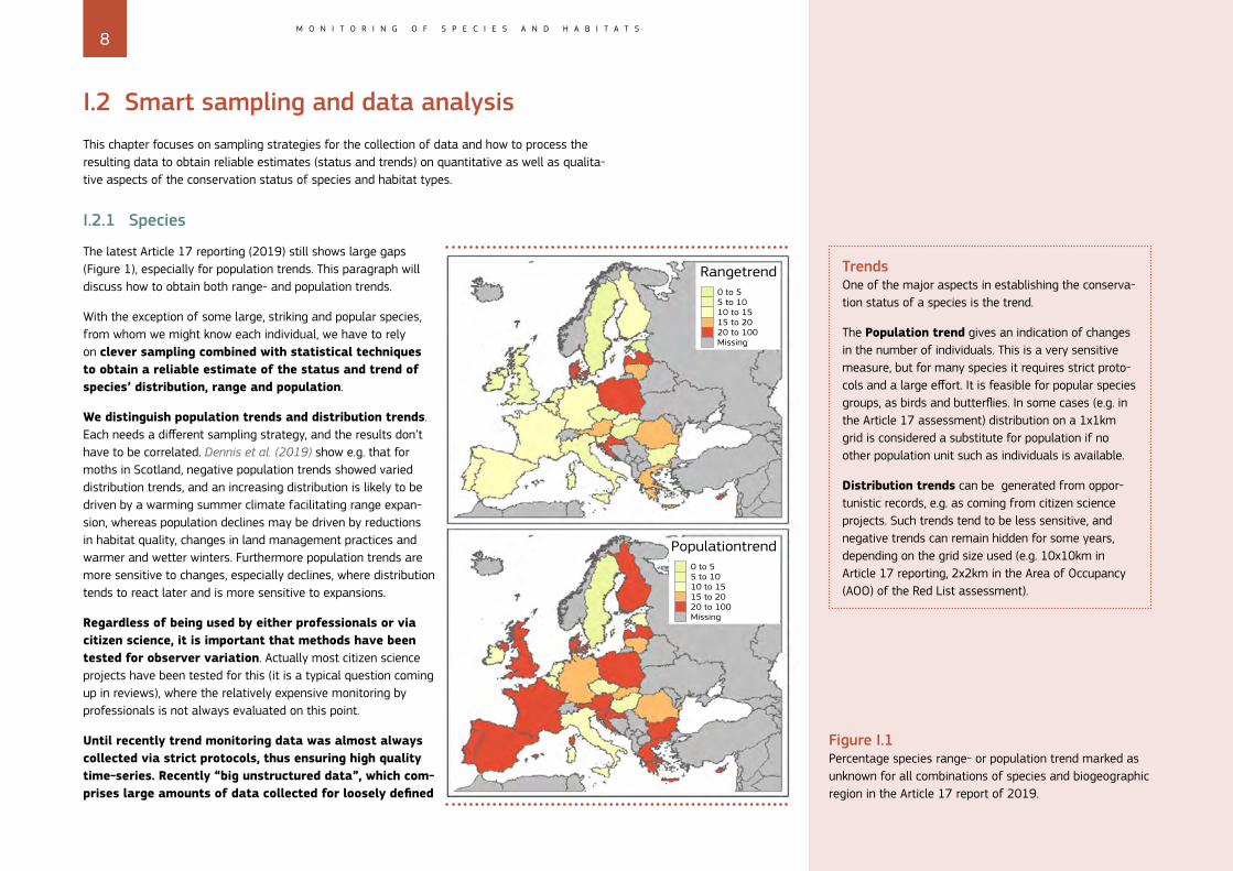
The latest Article 17 reporting (2019) still shows large gaps (Figure 1), especially for population trends. This paragraph will discuss how to obtain both range- and population trends.
With the exception of some large, striking and popular species, from whom we might know each individual, we have to rely on clever sampling combined with statistical techniques to obtain a reliable estimate of the status and trend of species’ distribution, range and population.
We distinguish population trends and distribution trends. Each needs a different sampling strategy, and the results don’t have to be correlated. Dennis et al. (2019) show e.g. that for moths in Scotland, negative population trends showed varied distribution trends, and an increasing distribution is likely to be driven by a warming summer climate facilitating range expan-sion, whereas population declines may be driven by reductions in habitat quality, changes in land management practices and warmer and wetter winters. Furthermore population trends are more sensitive to changes, especially declines, where distribution tends to react later and is more sensitive to expansions.
Regardless of being used by either professionals or via citizen science, it is important that methods have been tested for observer variation. Actually most citizen science projects have been tested for this (it is a typical question coming up in reviews), where the relatively expensive monitoring by professionals is not always evaluated on this point.
Until recently trend monitoring data was almost always collected via strict protocols, thus ensuring high quality time-series. Recently “big unstructured data”, which com-prises large amounts of data collected for loosely defined
Trends One of the major aspects in establishing the conserva-tion status of a species is the trend.
The Population trend gives an indication of changes in the number of individuals. This is a very sensitive measure, but for many species it requires strict proto-cols and a large effort. It is feasible for popular species groups, as birds and butterflies. In some cases (e.g. in the Article 17 assessment) distribution on a 1x1km grid is considered a substitute for population if no other population unit such as individuals is available.
Distribution trends can be generated from oppor-tunistic records, e.g. as coming from citizen science projects. Such trends tend to be less sensitive, and negative trends can remain hidden for some years, depending on the grid size used (e.g. 10x10km in Article 17 reporting, 2x2km in the Area of Occupancy (AOO) of the Red List assessment).
Figure I.1 Percentage species range- or population trend marked as unknown for all combinations of species and biogeographic region in the Article 17 report of 2019.
Rangetrend0 to 55 to 1010 to 1515 to 2020 to 100Missing
Populationtrend0 to 55 to 1010 to 1515 to 2020 to 100Missing
9M O N I T O R I N G O F S P E C I E S A N D H A B I T A T S
“observatory purposes”, have become an important source of biodiversity data. So far such opportunistic citizen science data can only be used for distribution trends if rigorous models correct for observation, reporting and detection biases (Bayraktarov et al., 2019). Big unstructured data, although abundant, typically have a high level of noise to signal ratio which obscures the signal on real trends (Cunningham & Lindenmayer, 2017). Moreover, data collec-tion without specified (testable) objectives may not measure the “correct” variables to answer questions about biodiversity (Bayraktarov et al., 2019).
Population
a. Population size
Establishing population size in exact numbers can be a challenge. Distance sampling and territory mapping are survey techniques for estimating bird abundance (Bibby et al., 2000; Buckland et al., 2001). But for other, often smaller, animals and plants, it can be difficult or even impossible to measure the exact population size, even if they occur in small and closed populations without contact to other populations. As a consequence in the latest version of the Article 17 reporting for the Habitats Directive, the reporting unit for many species was changed to 1x1km (DG Environment, 2017). But even then this can rely heavily on sampling intensity. Where relevant and possible detection probability should be taken into account, e.g. by occupancy modelling (see for more details the next paragraph). For pelagic birds, cetaceans and marine reptiles line transect surveys in a regular pattern (e.g. Panigada et al., 2011) in combination with distance sampling make it possible to get population estimates of some of the more common species. Aerial surveys proved to be more efficient than ship surveys, allowing more robust estimates (Panigada et al., 2011). When applying such tech-niques it is important to take detectability into account. For some cetacean species, mark-re-capture methods can be applied using photo-identification of recognizable individuals (Evans & Hammond, 2004). Anyway the power to detect trends in cetaceans is low. Tyne et al. (2016) showed in a test case with a Spinner dolphin that it would take nine years to detect a 5% annual change in abundance (with a power of 80%), so if the trend was a decline, the population would have decreased by 37% prior to detection of a significant decline.
Most of the fish and lampreys listed in the Annexes of the Habitats Directive occurring in the sea are anadromous (or have anadromous populations), i.e. they migrate between rivers (where they spawn) and the sea. As there are many barriers in most rivers, migrant fish can be monitored at those sites.
b. Population trend
Although it can be a challenge to measure the exact population size, there are good techniques available to measure changes in population size: the population trend. For population trends regular counts (one way or the other) are the basis. Counts can be
Distance sampling = During a transect walk the distance to the object is estimated.
Territory mapping = Territories are distinguished after multiple visits.
10M O N I T O R I N G O F S P E C I E S A N D H A B I T A T S
performed by transects, plots, camera-traps etc. It is important that such methods are harmonised, with each country delivering the same parameters (e.g. the population trend and the confidence interval), not necessarily standardised: methods may differ in detail (the trend can e.g. be produced from transect counts in one country, and camera-traps in another country). The method should guarantee that the results (the trends and their statistical uncertainty) can be combined for use at a higher (e.g. European or EU) level. In the calculation of European bird trends (PECBMS: pecbms.info) and butterfly trends (eBMS via ABLE: butterfly-monitoring.net) this is already incorporated (see also the example in the side box).
This can be achieved by:
» Ensuring that the protocols are well described and maintained, and can deliver the data needed.
» Setting up a method to account for the differences in the results, and combining them at a larger scale or further back in time (when e.g. new techniques were not yet available).
In this way new techniques and methods can be combined with older, long time-series, thus enabling a view back into time but still use new innovative techniques. However calibration is needed when detection probabilities change.
Although statistical techniques offer the possibility to combine many short time-series to produce a long-term trend (see e.g. Hallmann et al., 2017), the power of monitoring is in long time-series with regular counts. Such counts are made on sample points, transects or plots (fur-ther referred to as sample points). Sample points can be arranged in different ways:
» Random: locations are chosen at random, e.g. in the Wider Countryside Butterfly Survey.
» Grid: locations are in a strict grid. A typical example is the Biodiversity Monitoring Swit-zerland, where species, habitats and water is monitored in a regular grid. In some areas (Kantons) the density is higher than in others, because of additional funding. At sea these can also be a regular pattern of transects (see e.g. Panigada et al., 2011).
» Free choice: participants can choose their own favoured location. As good as always these will be volunteers, professionals can be directed to random, grid or targeted monitoring locations.
» Targeted: monitoring focuses on specific sites, species or habitats, e.g. species mentioned in the annexes of the Habitats Directive or other (policy) relevant species (e.g. in Flanders).
Random and grid based approaches have the advantage of delivering reliable trends, where no weighting of stratification is necessary. However rare species or habitats are easily missed and as a result are underrepresented in the network, and often no trends can be calculated for such rare species, which often are policy-relevant (e.g. because they are mentioned in the annexes of the Habitats Directive). Furthermore random and grid-based networks are expensive if counts by
European bird monitoring data: harmonised, not standardisedFor the PanEuropean Common Bird Monitoring Scheme (PECBMS) coordinators of national bird monitoring schemes deliver their national results to the PECBMS coordination unit annually. The data delivered are:
» the national yearly indices per species,
» the all-sites yearly totals (= the sum of birds counted across all sites per year) and their stan-dard errors,
» the covariances between the yearly figures.
The method to come to the national data can differ from country to country (the field methods do not have to be standardised, some countries apply e.g. the labour-intensive territory mapping, while others may use transect counts), but as the national output is har-monised (all countries deliver the same set of data) they can be used to calculate European trends.
For more details see pecbms.info/methods/pecbms-methods
11M O N I T O R I N G O F S P E C I E S A N D H A B I T A T S
people have to be made: volunteers tend to focus on attractive sites, as nature reserves, mean-ing many points have to be counted by professionals. However for automated methods (e.g. camera-traps) this is not an issue, even if a large number of potential volunteers is available (e.g. in the United Kingdom). Automated methods can also be a good alternative for the lack of volunteers or (funding for) professional experts for less known species groups (e.g. bees), but these techniques are new and will need some time to further develop. However the first steps on using camera-traps with image recognition through artificial intelligence (AI) have been made, and in the coming years these will become more generally available.
Free-choice networks are mostly used in citizen-science based monitoring: volunteers can choose their own sites. This will lead to an overrepresentation of sites in nature reserves and urban areas. Such data can be corrected by stratified weighting for the more common and widespread species, as long as there is enough data from unattractive sites (usually large-scale agricultural areas). Advantage of this system is that rare and policy relevant species are favoured, and in general there will be enough sites for those species.
Targeted monitoring, usually by professionals (but not always, see e.g. www.meetnetten.be), can be an effective way to get population trends of a chosen set of species. It can be costly (certainly if there are many species and many locations), and strict quality control is needed, as detection probabilities for many species are so low, that multiple visits during a year are needed, which is not always done. For species for which the detection probability is known (e.g. butterflies and dragonflies; Van Strien et al., 2013) we can calculate the minimal number of visits (in the case of butterflies and dragonflies: at least three per season), and this will be even more for shy or night-active species (for whom the detection probability will be even lower), for which often experience and a lot of expert knowledge is needed to find them. Another disadvan-tage is that only target-species are counted, and trends in other species will be missed. Also the results cannot be used for community indicators (e.g. Ellenberg indicators in plants).
For the calculation of population trends several techniques are available, usually based on a Generalized Linear Models (GLM) or Generalised linear mixed models (GLMM) with poisson dis-tribution, such as TRIM (Pannekoek & Van Strien, 2001, now available as R-package rtrim) and the Generalized Abundance Index (Dennis et al., 2016).
Joining efforts by creating a central data and information point can be an effective way to improve the consistency and harmonisation of monitoring methods across the EU. For birds this was created by the European Bird Census Council, who run the Pan-European Common Bird Monitoring Scheme (PECBMS) since 2002. Recently the ABLE-project (Assessing Butterflies in Europe) started, building on the European Butterfly Monitoring Scheme (eBMS) with the ambition to form a central database for all butterfly and moth monitoring counts in Europe. When this project is finished in December 2020, there should be butterfly-monitoring in most EU countries.
It would be good to build on these examples and experiences and start up similar initiatives for other species groups.
12M O N I T O R I N G O F S P E C I E S A N D H A B I T A T S
Species distributionIn general distribution maps (giving the distribution, often in units as 1x1km squares or 10x10km squares) and distribution trends are not based on systematic counts, but on opportunistic data. Long-term monitoring schemes provide high-quality data, often on an annual basis, but are taxonomically and geographically restricted. By contrast, opportunistic biological records are relatively unstructured but vast in quantity (Isaac et al., 2014). With the growth of online portals, such as ebird.org, observation.org and iNaturalist.org, usually with as-sociated smartphone apps, next to local and national biodiversity databases (e.g. artportalen.se or ndff.nl), the number of records has grown almost exponentially in recent years. Some of these online portals lend their data to gbif.org, the Global Biodiversity Information Facility, which held 1.3 billion records in June 2019. GBIF data is freely available for download for research and conservation. One of the main flaws is that validation and quality control depends on the da-ta-source, and as such part of the data can be unreliable. In some countries sharing of distribu-tion data is not encouraged by the Member States, and as a result the data which is available is limited and divided over several data sources. In other countries holiday records from natural-ists from other countries could make a considerable difference. Without the uploading of such records to GBIF, or downloading them from GBIF, a lot of valuable distribution data might not be used. The EU could play a role in encouraging all Member States to make distribution data available via GBIF.
Distribution data tends to be presence/absence (or better: detection/not detection). Although part of the data can be real counts, without a protocol or clear method description, such counts cannot be used easily for (range) trends. Isaac et al. (2014) compared a set of methods that employ data filtering criteria and/or correction factors to deal with variation in recorder activity. They found that simple methods produce biased trend estimates, and/or had low power, and should be avoided. No method was wholly unaffected by all forms of variation in recorder activ-ity, although some performed well enough to be useful. Sophisticated methods that model the data collection process offer the greatest potential to estimate timely trends, notably Frescalo and occupancy–detection models (see Isaac et al., 2014 for more details).
It should be noted that especially the most sophisticated models for distribution trends are also ‘data-hungry’ and require a lot of input. Next to that there is a minimum quality of visits required. Ideally participants record all species of a species group. This works well in some species groups (e.g. butterflies), but fails in other species groups, most notably birds, where re-corders usually don’t have the habit of producing complete species lists. Future sampling therefore should concentrate on ways of enhancing the quality of species lists per visit.
In some countries bird atlases have been produced following strict protocols (e.g. Schekkerman et al., 2012), which allow estimates of the population size as well as for comparison between periods and thus establishing species distribution trends. However such atlases are very la-bour-intense and only possible in a limited number of counties and species-groups.
From observations to distribution map to trends in distribution: the Netherlands as an exampleDistribution data is collected in different ways. To illustrate the magnitude, we will give an example using the information available on the Grayling (Hipparchia semele) in the Netherlands in 2017. Here this is a char-acteristic butterfly of dry heathland and coastal dunes.
Targeted data collection, following a protocol:
Repeated surveys: every six years almost all nature reserves (including all Natura 2000 areas) are investi-gated by professionals on the distribution (at least on a 100m scale) of a group of species (birds, plants, and a selection of butterflies, dragonflies and grasshoppers). 1490 records of the Grayling were recorded in 2017 under the SNL-protocol.
Population monitoring: following a strict protocol for population monitoring by volunteers, this also gener-ates distribution data. 407 counts of the Grayling were recorded in 2017 for population monitoring. Targeted distribution research, especially for rare and/or hard to detect species, often on the Habitats Directive. As the Grayling is not on the Habitats Directive, no records were collected in the Netherlands under this project.
Opportunistic records: almost all occasional observa-tions in the Netherlands are entered via one of the on-line portals (waarneming.nl, telmee.nl), most of them via a smartphone-app. In 2017 the Grayling was recorded on 2425 occasions as single opportunistic record.
After validation all observations are included in the National Database Flora and Fauna (NDFF). Validation is based on the following principles:
Automatic validation: all records run through a script which checks for distribution (is the observation at or near a known location), time of year (does this species occur in this stage in this time of the year) and ...
13M O N I T O R I N G O F S P E C I E S A N D H A B I T A T S
For anadromous fish and lampreys, often recorded only in a few localities in the river systems, e.g. the spawning grounds or at fish passes, the complete migration route in the rivers from the mouths in the sea to the highest know stretches should be included in the distribution (DG Environment, 2017).
Range and range trend are special cases of distribution and distribution trend, as they are based on 10x10km grid cells. Range is defined as ‘the outer limits of the overall area in which a habitat type or species is found at present’ and it can be considered as an envelope within which areas actually occupied occur. The range should be calculated based on the map of the actual distribution using a standardised algorithm. A standardised process is needed to ensure repeatability of the range calculation in different reporting rounds (DG Environment, 2017). The method for compiling range and range trend is described in detail in DG Environment (2017). Advantages and disadvantages are comparable to other measures of distribution and distribu-tion trend.
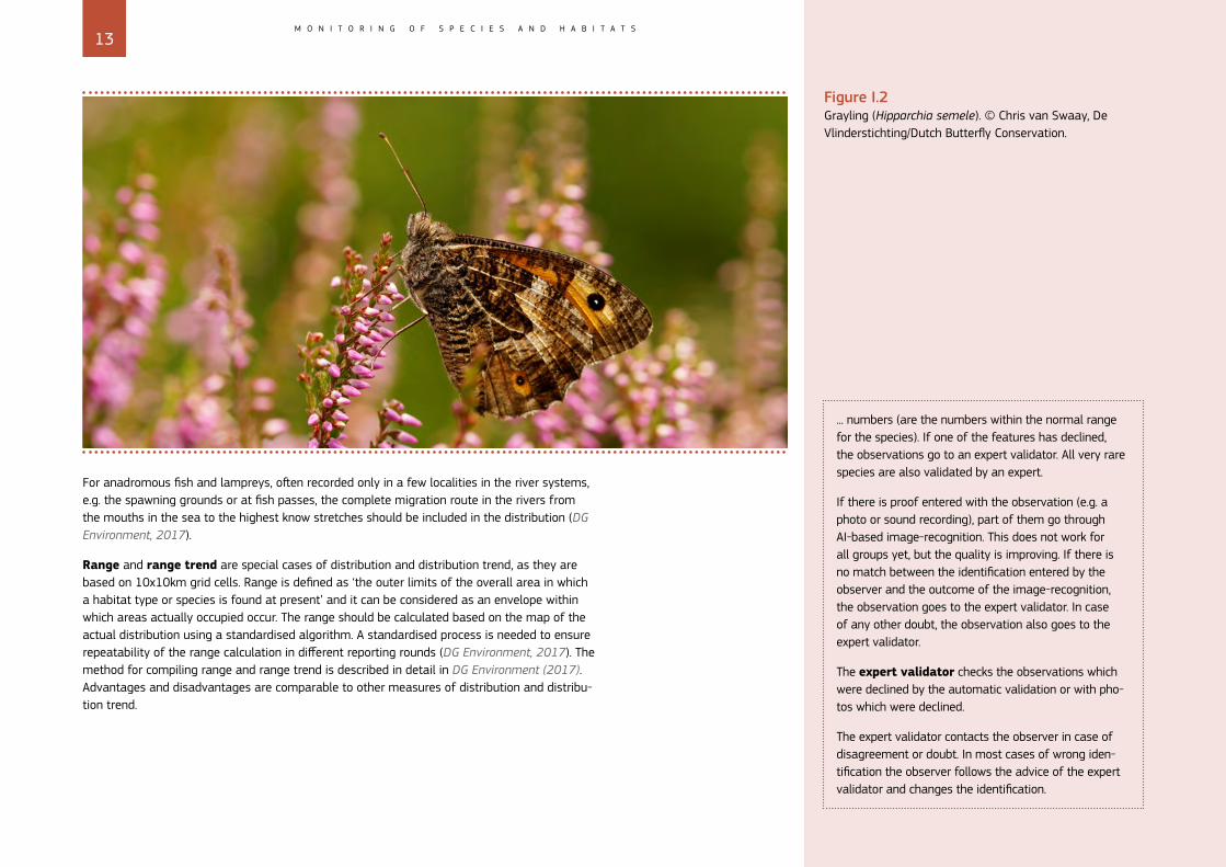
Figure I.2 Grayling (Hipparchia semele). © Chris van Swaay, De Vlinderstichting/Dutch Butterfly Conservation.
... numbers (are the numbers within the normal range for the species). If one of the features has declined, the observations go to an expert validator. All very rare species are also validated by an expert.
If there is proof entered with the observation (e.g. a photo or sound recording), part of them go through AI-based image-recognition. This does not work for all groups yet, but the quality is improving. If there is no match between the identification entered by the observer and the outcome of the image-recognition, the observation goes to the expert validator. In case of any other doubt, the observation also goes to the expert validator.
The expert validator checks the observations which were declined by the automatic validation or with pho-tos which were declined.
The expert validator contacts the observer in case of disagreement or doubt. In most cases of wrong iden-tification the observer follows the advice of the expert validator and changes the identification.
14M O N I T O R I N G O F S P E C I E S A N D H A B I T A T S
Habitat for speciesA species needs a sufficiently large area of habitat of suitable quality and spatial distribution to survive and flourish. To measure it we should take into account (DG Environ-ment, 2017):
» physical and biological requirements of the species; this includes prey, pollinators, etc.;
» all stages of its life cycle are covered and seasonal variation in the species’ requirements is reflected.
Monitoring the size, quality and spatial arrangement of the habitat of a species is not only difficult, but also subject to changes in the species’ preferences: as a result of climate change some species have changed their habitat preferences and widened or narrowed down their range of preferred habitats. Although in some cases vegetation can be used as a proxy for habitat quality, this often neglects other requirements of species, i.e. food, shelter, interac-tions with other species, etc.
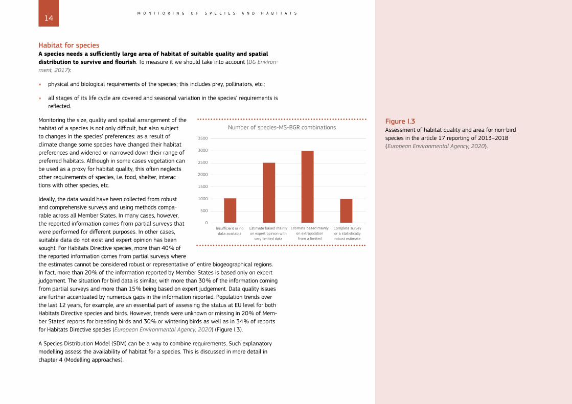
Ideally, the data would have been collected from robust and comprehensive surveys and using methods compa-rable across all Member States. In many cases, however, the reported information comes from partial surveys that were performed for different purposes. In other cases, suitable data do not exist and expert opinion has been sought. For Habitats Directive species, more than 40 % of the reported information comes from partial surveys where the estimates cannot be considered robust or representative of entire biogeographical regions. In fact, more than 20 % of the information reported by Member States is based only on expert judgement. The situation for bird data is similar, with more than 30 % of the information coming from partial surveys and more than 15 % being based on expert judgement. Data quality issues are further accentuated by numerous gaps in the information reported. Population trends over the last 12 years, for example, are an essential part of assessing the status at EU level for both Habitats Directive species and birds. However, trends were unknown or missing in 20 % of Mem-ber States′ reports for breeding birds and 30 % or wintering birds as well as in 34 % of reports for Habitats Directive species (European Environmental Agency, 2020) (Figure I.3).
A Species Distribution Model (SDM) can be a way to combine requirements. Such explanatory modelling assess the availability of habitat for a species. This is discussed in more detail in chapter 4 (Modelling approaches).
Figure I.3 Assessment of habitat quality and area for non-bird species in the article 17 reporting of 2013–2018 (European Environmental Agency, 2020).
Number of species-MS-BGR combinations
3500
3000
2500
2000
1500
1000
500
0Insufficient or no data available
Estimate based mainly on expert opinion with
very limited data
Estimate based mainly on extrapolation from a limited
amount of data
Complete survey or a statistically robust estimate
15M O N I T O R I N G O F S P E C I E S A N D H A B I T A T S
I.2.2 Habitat types
This subchapter gives an overview of sampling strategies and data analysis methods that are/can be used for the monitoring of the habitat types of Annex I of the Habitats Directive.
Habitat typologiesThere is an interpretation manual of the European Union Habitats (EU, 2013). This manual forms the basis for all habitat classification and is regularly updated, e.g. with the expansion of the EU Member States. Although there is this common habitat typology, the interpretation of the habitat types of Annex I of the Habitats Directive differs per Member States and even within a MS (Evans, 2010).
For the Habitat Directive Article 17 reporting information is needed on the area (status and trends), the distribution (status and trends) and the structure and function or ‘quality’ of the habitat types on national and biogeographical level. For site management and protection similar but more detailed information is needed on these parameters.
Lengyel et al. (2008b) compared the different approaches and methods applied by MS to moni-tor habitat types, based on the descriptions (meta data) of habitat monitoring schemes collected within the EUMON-project and stored and maintained in the EUMON database. Lengyel (2008a) sees promising developments in habitat monitoring, amongst others that most schemes monitor distribution and species composition of habitats as well environmental parameters. The main weakness is that in more than half of the schemes it is not clear how the collected data are analysed as this is not described in the monitoring schemes. Advanced statistics may be used infrequently because in most schemes sampling sites are selected based on expert/person-al knowledge rather than predefined criteria derived from a sampling theory. Lengyel (2018) pleads for benchmarking of monitoring of species and habitat types. By means of sharing and comparing different data and sampling analysis techniques e.g. between the Mem-ber States or site managers one can learn from each other and step by step improve these methods and possibly qualify or certify methods. As explained in the former chapter on species, it is not necessary to use the same methodologies as long as the protocols are well described and lead to a similar outcome that can be compared.
Since 2008 developments have been made by the MS in habitat monitoring, but an extensive review of the current state of the art is missing. Ellwanger (2018) made a more recent com-parison between the monitoring approaches of a selection of MS and concludes that there are considerable differences in terms of data sampling (e.g. sampling size) and data analysis (e.g. statistical robustness).
Habitat areaHabitat area is often monitored based on repeated/ sequential habitat mapping. Different approaches for habitat mapping are used, varying from field mapping to the
16M O N I T O R I N G O F S P E C I E S A N D H A B I T A T S
interpretation of aerial photographs and automated classification of remote sensing imagery. Often a combination of different methods is applied depending on the habitat type or group of habitat types. The Czech Republic for example have interpreted Habitats Directive Annex I habitats by the national system of biotopes and carried out an extensive field mapping of the entire Czech Republic in the fine-scale 1:10.000 (Guth & KuČera, 2005). A large amount of field data was collected of all biotopes, mainly about their distribution, spatial dimensions, and qualities.
Due to differences in the interpretations e.g. in the field or of the aerial photographs, trends in habitat area are often difficult to assess or uncertain and inaccurate. As Lengyel (2008a) concludes the information on how the data is analysed (meta data) to derive trends in area of habitat types is often missing in the national report of the MS. Therefore the uncertainty of the trends is unclear. A system with qualifiers as is being used by IPBES might be applied, but it requires transparency in the methods being applied by the different member states. It is up to the Member State to indicate the quality class without further information.
Remote sensing techniques might offer means to harmonise the data collection on the area and as well the distribution of habitat types as these methods are (partly) automated and can be standardised to a certain extent. Not all habitat types can be that easily detected by means of remote sensing so field work is often necessary.
Habitat distributionHabitat distribution is estimated based on mapping as well as modelling. The problem is that habitat maps are often only available of a selection of sites and not on a national or bio-geographical scale. Habitat distribution modelling can give a more complete estimate of habitat distribution (see chapter I.4).
Habitat structure and functionStructure and function is the key aspect for the assessment of the conservation status of habitat types as it provides information on the ‘quality’ of the habitats (Ellwanger et al., 2018).
The assessment of habitat quality according to the requirements of the EC is based on the criteria habitat structures, habitat functions and typical species. Structures are considered to be the physical components of a habitat type. These will often be formed by assemblages of species (both living and dead), but can also include abiotic features, such as gravel used for spawning. Functions are the ecological processes occurring at a number of tem-poral and spatial scales and they vary greatly between habitat types. Typical species are those which mainly occur in a habitat type or at least in a subtype of a variant of a habitat type (DG Environment, 2017). The species composition of a given habitat type may vary geographically.
Individual attributes or sub-criteria have to be selected for each habitat type to as-sess habitat structure and function (habitat quality). The data collected on the different

17M O N I T O R I N G O F S P E C I E S A N D H A B I T A T S
criteria and/or subcriteria of the aspect structure and function needs to be aggregated and weighted (similar to the final assessment of the conservation status of a habitat type).
Ellwanger (2018) concludes that most of the monitoring approaches (of the MS included in his study) for assessing the structure and function of habitat types are based at least partially on sampling. The number of sampling areas depends on the occurrence of the habitat type (rare vs widespread) and other ecological and methodological factors, as well as efforts and costs. Each MS selects the sample plots differently. Overall, most MS conduct at least a partly systematic selection based on the distribution, the size (area) and characteristics of habitat types and/or other factors. Most MS used permanent plots, include area within and outside the Natura 2000 network and have standard assessment schemes.
None of the MS included in the study of Ellwanger (2018) made a statement on theoretical statistical strength of the samples for monitoring. This corresponds to what Lengyel (2008) concluded ten years before. There is a lack of a proper description of the data collection and analysis protocols that are used and on the certainty the information derived from these data.
a. Typical species
Concerning the typical species most MS investigate plant species only (Ellwanger, 2018), most probably because plants are quite easily linked to habitat types (the habitat typology is heavily based on plant communities), whereas for fauna species it is much more difficult. Some fauna species depend on more than one habitat type (e.g. for breeding, foraging, resting etc.) which is much more difficult. In case animals species are in-vestigated the most frequently, used animal groups are birds, butterflies and beetles. This is probably due to the fact that these species groups are relatively easy to de-tect and recognize and often observed by large volunteers networks. In The Netherlands a method has been developed to assess structure and function of habitat types based on trends in the distribution of typical plant species (Janssen et al., 2020).
b. Aggregation methods
There are different approaches for the aggregation of the data (assessment criteria) for the purpose of structure and function assessments. For each habitat type an assess-ment needs to be performed of the area (km2) in good condition. As the condition is defined by different sub-parameters there should be a weighing between these sub-parameters as well a threshold for good condition. Measurements are being made at single plot and at site level. These measurements need to be aggregated on the level of a bio-geographical region. Different approaches are being followed by the Member States.
18M O N I T O R I N G O F S P E C I E S A N D H A B I T A T S
I.3 Observation technologiesThis chapter focuses on innovative techniques for the observation of species and habitat types. It is not meant to be complete. A selection of techniques has been made and examples are given for certain species and habitat types. There is no description on data collection and analysis techniques in this chapter as this has been described in chapter 2, but different type of observations might require different sampling and data analysis methods. The costs of the different techniques are missing in this chapter. A lot of these techniques are still being developed (e.g. the automated detection of species on images) and therefore more experi-mental, which makes it difficult to estimate the costs of an operational system.
I.3.1 Species
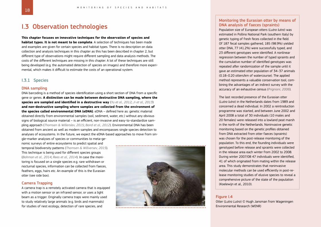
DNA samplingDNA barcoding is a method of species identification using a short section of DNA from a specific gene or genes. A distinction can be made between destructive DNA sampling, where the species are sampled and identified in a destructive way (Yu et al., 2012; Ji et al., 2013) and non-destructive sampling where samples are collected from the environment of the species called environmental DNA (eDNA). eDNA – defined here as: genetic material obtained directly from environmental samples (soil, sediment, water, etc.) without any obvious signs of biological source material – is an efficient, non-invasive and easy-to-standardize sam-pling approach (Thomsen & Willerslev, 2015; Baird et al., 2012). Environmental DNA has been obtained from ancient as well as modern samples and encompasses single species detection to analyses of ecosystems. In the future, we expect the eDNA-based approaches to move from sin-gle-marker analyses of species or communities to meta-ge-nomic surveys of entire ecosystems to predict spatial and temporal biodiversity patterns (Thomsen & Willversev, 2015). This technique is being used for different species groups (Bohman et al., 2014; Rees et al., 2014). In case the moni-toring is focused on a single species e.g. rare withdrawn or nocturnal species, information can be collected from faeces, feathers, eggs, hairs etc. An example of this is the Eurasian otter (see side box).
Camera Trapping A camera trap is a remotely activated camera that is equipped with a motion sensor or an infrared sensor, or uses a light beam as a trigger. Originally camera traps were mainly used to study relatively large animals (e.g. birds and mammals) for studies of nest ecology, detection of rare species, and
Monitoring the Eurasian otter by means of DNA analysis of faeces (spraints) Population size of European otters (Lutra lutra) was estimated in Pollino National Park (southern Italy) by genetic typing of fresh feces collected in the field. Of 187 fecal samples gathered, 185 (98.9%) yielded otter DNA, 77 (41.2%) were successfully typed, and 23 different genotypes were identified. A nonlinear regression between the number of typed spraints and the cumulative number of identified genotypes was repeated after randomization of the sample until it gave an estimated otter population of 34–37 animals (0.18–0.20 otters/km of watercourse). The applied method represents a valuable conservation tool, com-bining the advantages of an indirect survey with the accuracy of an exhaustive census (Prignioni, 2006).
The last recorded presence of the Eurasian otter (Lutra lutra) in the Netherlands dates from 1989 and concerned a dead individual. In 2002 a reintroduction programme was started, and between June 2002 and April 2008 a total of 30 individuals (10 males and 20 females) were released into a lowland peat marsh in the north of the Netherlands. Noninvasive genetic monitoring based on the genetic profiles obtained from DNA extracted from otter faeces (spraints) was chosen for the post-release monitoring of the population. To this end, the founding individuals were genotyped before release and spraints were collected in the release area each winter from 2002 to 2008. During winter 2007/08 47 individuals were identified, 41 of which originated from mating within the release area. This study demonstrates that noninvasive molecular methods can be used efficiently in post-re-lease monitoring studies of elusive species to reveal a comprehensive picture of the state of the population (Koelewijn et al., 2010).
Figure I.4 Otter (Lutra Lutra) © Hugh Jansman from Wageningen Environmental Research (WENR)
19M O N I T O R I N G O F S P E C I E S A N D H A B I T A T S
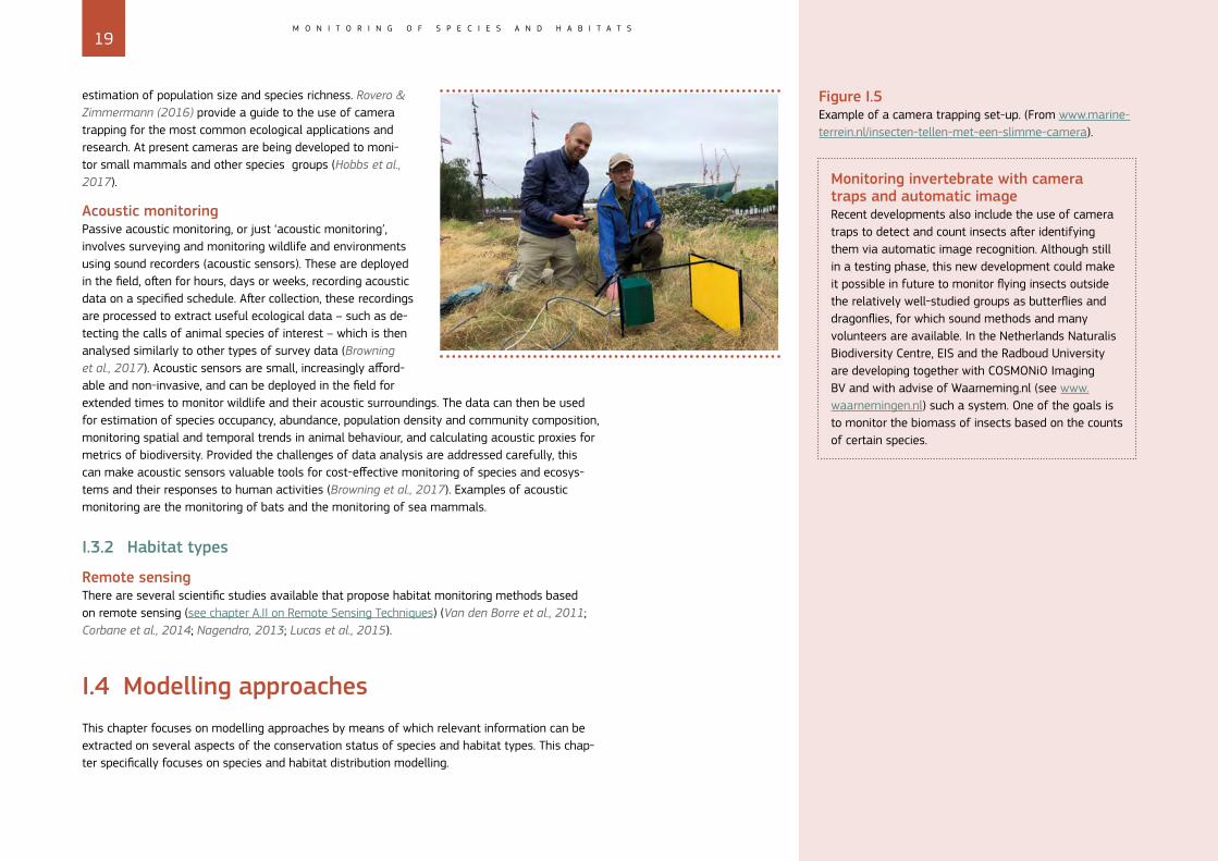
estimation of population size and species richness. Rovero & Zimmermann (2016) provide a guide to the use of camera trapping for the most common ecological applications and research. At present cameras are being developed to moni-tor small mammals and other species groups (Hobbs et al., 2017).
Acoustic monitoringPassive acoustic monitoring, or just ‘acoustic monitoring’, involves surveying and monitoring wildlife and environments using sound recorders (acoustic sensors). These are deployed in the field, often for hours, days or weeks, recording acoustic data on a specified schedule. After collection, these recordings are processed to extract useful ecological data – such as de-tecting the calls of animal species of interest – which is then analysed similarly to other types of survey data (Browning et al., 2017). Acoustic sensors are small, increasingly afford-able and non-invasive, and can be deployed in the field for extended times to monitor wildlife and their acoustic surroundings. The data can then be used for estimation of species occupancy, abundance, population density and community composition, monitoring spatial and temporal trends in animal behaviour, and calculating acoustic proxies for metrics of biodiversity. Provided the challenges of data analysis are addressed carefully, this can make acoustic sensors valuable tools for cost-effective monitoring of species and ecosys-tems and their responses to human activities (Browning et al., 2017). Examples of acoustic monitoring are the monitoring of bats and the monitoring of sea mammals.
I.3.2 Habitat types
Remote sensingThere are several scientific studies available that propose habitat monitoring methods based on remote sensing (see chapter A.II on Remote Sensing Techniques) (Van den Borre et al., 2011; Corbane et al., 2014; Nagendra, 2013; Lucas et al., 2015).
I.4 Modelling approachesThis chapter focuses on modelling approaches by means of which relevant information can be extracted on several aspects of the conservation status of species and habitat types. This chap-ter specifically focuses on species and habitat distribution modelling.
Monitoring invertebrate with camera traps and automatic image Recent developments also include the use of camera traps to detect and count insects after identifying them via automatic image recognition. Although still in a testing phase, this new development could make it possible in future to monitor flying insects outside the relatively well-studied groups as butterflies and dragonflies, for which sound methods and many volunteers are available. In the Netherlands Naturalis Biodiversity Centre, EIS and the Radboud University are developing together with COSMONiO Imaging BV and with advise of Waarneming.nl (see www.waarnemingen.nl) such a system. One of the goals is to monitor the biomass of insects based on the counts of certain species.
Figure I.5 Example of a camera trapping set-up. (From www.marine-terrein.nl/insecten-tellen-met-een-slimme-camera).
20M O N I T O R I N G O F S P E C I E S A N D H A B I T A T S
I.4.1 Definition of modelling
Models are a more and more popular way to describe the relationships between a species' distribution and/or trend, and the underlying drivers. Practically a model is a set of mathemat-ical equations or logical rules that link a biodiversity variable of interest to one or more other variables e.g. environmental drivers (Ferrier et al., 2017).
Explanatory modellingExplanatory modelling is conducted across space alone, at a single point in time (usually the present). Explanatory modelling of correlations, or associations, between a biodiversity-response variable observed at a sample of geographical locations, and a set of predictor variables mea-sured, or estimated, at these same locations, can help to shed light on the relative importance of different drivers in determining spatial patterns in biodiversity, and on the form (shape) of these relationships. The fitting of correlative species distribution models (SDMs) relating obser-vations of presence, presence-absence, or abundance of a given species to multiple environ-mental variables (e.g., climate, terrain, soil, land-use variables) is probably the best known, and most widely applied, manifestation of such data analysis (Ferrier et al., 2017).
Predictive modellingThe use of modelling to predict potential changes in biodiversity into the future as a function of ongoing impacts of environmental drivers (e.g. climate and land-use change), is called predictive modelling. Such modelling poses special challenges, as there is usually considerable uncertain-ty associated with the future trajectories of relevant environmental drivers, which themselves will be affected by socio-economic events and decisions that are yet to occur, and are therefore highly unpredictable. These uncertainties are often addressed through the use of scenarios, i.e. multiple plausible trajectories from environmental drivers, that account for the reality that not just one, but many, futures are possible (van Vuuren et al., 2012). Model-based biodiversity pro-jections under plausible scenarios of change in key drivers can contribute significantly to policy agenda setting, by helping to characterise and communicate the potential magnitude of ongoing change in biodiversity, and therefore the need for action. By extending scenarios to further consider the effects of alternative policy or management interventions, such projections can also play an important role in decision support, i.e. helping policy-makers, planners and managers to choose between possible actions for addressing the problem at hand, by modelling the differ-ence that each of these alternatives is expected to make to projected outcomes for biodiversity (Cook et al. 2014; Ferrier et al., 2017).
Models In general models are developed using data available from the (recent) past. Such models describe the relationship between variables (e.g. environmental pressures) and population size, distribution or trend of a species. Such models are called explanatory models (Shmueli, 2010).
Once such explanatory models have been developed, and the relationship of interest is known, as are observed or estimated values of the relevant predictor variables, these can be combined to predict previously unknown values of the biodiversity-response vari-able. Such models are called predictive models (Shmueli, 2010). A typical example of such predictive models are those describing the expected future tem-peratures under several climate scenarios.
21M O N I T O R I N G O F S P E C I E S A N D H A B I T A T S
I.4.2 Species distribution modelling
Species distribution modelling (SDM) uses computer algorithms to predict the distribution of a species across geographic space and time using environmental data (wikipedia.org). Further-more it generates functions or graphs to describe the relationship between the occurrence of the species and the environmental variable. Environmental data almost always includes climatic variables (e.g. temperature, precipitation) as well as other variables such as soil, land cover and pressure variables (e.g. Nitrogen deposition). These models can help to understand how environmental conditions influence the occurrence or abundance of a species, as well as for predictive purposes.
After building an SDM they can be used as predictive models, e.g. for species’ future distribu-tions under climate change scenarios (for birds: Huntley et al., 2007; for butterflies: Settele et al., 2008; for bumblebees: Rasmont et al., 2015). The Bioscore program is another example (Hen-driks et al., 2016). BioScore 2.0 is a model which supports the analysis of potential impacts of future changes in human-induced pressures on European terrestrial biodiversity (e.g. mammals, vascular plants, breeding birds and butterflies).
Building SDMs relies on data. The type of data determines the outcomes and risks. Jetz et al. (2019) give an overview of the effects of different types of raw data to build SDMs for Essen-tial Biodiversity Variables (EBVs). They distinguish three major data types (incidental records, inventories over small or large areas and expert synthesis maps) which differ in spatiotemporal scope, in taxonomic scope, in the quality of the presence (+) and absence information (–) that they provide and in spatiotemporal specificity, which in turn determine the key characteristics that they can inform.
Although monitoring data has the advantage of generating spatiotemporally very reliable data as well as useful absences, they often represent small localities (e.g. plots, transects) and are heavily based towards relatively small parts of the world. As a consequence SDMs are usually based on either opportunistic incidental records or on atlas distribution data (e.g. Hagemeijer & Blair, 1997 for birds; Kudrna et al., 2011 for butterflies).
Several methods have been developed for building SDMs. Most of them are available as R-pack-age (e.g. dismo, TRIMmaps and Biomod2). Maxent is a standalone program especially useful for incidental records.
SDMs are especially useful to establish the area and quality of habitat for a species (as required in the Article 17 reporting).
I.4.3 Habitat distribution modelling
Habitat distribution models are similar to species distribution models, namely predictive models based on hypotheses as to how environmental factors control the distribution of habitats.
22M O N I T O R I N G O F S P E C I E S A N D H A B I T A T S
Guisan & Zimmermann (2000) present a review of predictive habitat distribution modelling. A variety of statistical models is currently in use such as Generalized Linear Models to Classi-fication Tree and Regression Tree. The spatial distribution is simulated of respectively terrestrial plants species, aquatic plants, terrestrial animal species, plant communities, vegeta-tion types, plant functional types, biomes and vegetation units of similar complexity.
Guisan & Zimmerman (2000) consider the following four main sources of environmental data (to predict habitat distribution):
» field surveys or observational studies
» printed or digitized maps
» remote sensing data
» maps obtained from GIS based modelling procedures
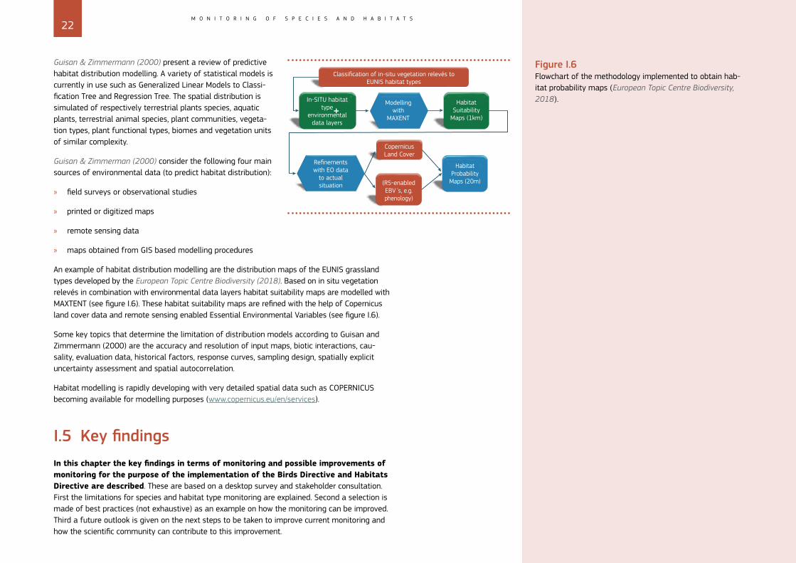
An example of habitat distribution modelling are the distribution maps of the EUNIS grassland types developed by the European Topic Centre Biodiversity (2018). Based on in situ vegetation relevés in combination with environmental data layers habitat suitability maps are modelled with MAXTENT (see figure I.6). These habitat suitability maps are refined with the help of Copernicus land cover data and remote sensing enabled Essential Environmental Variables (see figure I.6).
Some key topics that determine the limitation of distribution models according to Guisan and Zimmermann (2000) are the accuracy and resolution of input maps, biotic interactions, cau-sality, evaluation data, historical factors, response curves, sampling design, spatially explicit uncertainty assessment and spatial autocorrelation.
Habitat modelling is rapidly developing with very detailed spatial data such as COPERNICUS becoming available for modelling purposes (www.copernicus.eu/en/services).
I.5 Key findingsIn this chapter the key findings in terms of monitoring and possible improvements of monitoring for the purpose of the implementation of the Birds Directive and Habitats Directive are described. These are based on a desktop survey and stakeholder consultation. First the limitations for species and habitat type monitoring are explained. Second a selection is made of best practices (not exhaustive) as an example on how the monitoring can be improved. Third a future outlook is given on the next steps to be taken to improve current monitoring and how the scientific community can contribute to this improvement.
Classification of in-situ vegetation relevés toEUNIS habitat types
In-SITU habitattype
environmentaldata layers
Modellingwith
MAXENT
HabitatSuitability
Maps (1km)
Refinementswith EO data
to actualsituation
CopernicusLand Cover
(RS-enabledEBV́ s, e.g.phenology)
HabitatProbability
Maps (20m)
Figure I.6 Flowchart of the methodology implemented to obtain hab-itat probability maps (European Topic Centre Biodiversity, 2018).
23M O N I T O R I N G O F S P E C I E S A N D H A B I T A T S
I.5.1 Best practices / examples
Smart sampling and data analysisGood data and statistically robust trends require a serious investment of time and money. Depending on the culture in a country (in some countries the view on the use of volunteer data is very different than in others, see Bell et al. (2008)) and the availability of resources (either time or money) each country has to make its own decisions. Methods don’t necessarily have to be standardised, as long as they are scientifically sound and published in a peer-reviewed journal. New recent developments (e.g. occupancy modelling and Species Distribution models) offer new possibilities, but methods tend to be centred either around volunteer-based and professional-based solutions.
Volunteer-basedFor collecting species distribution-data (so also range-data, which is a special case of distribution-data) with volunteers, a user-friendly database, website and smartphone-app has to be setup, either nationally or by joining one of the major international ones (as iNaturalist.org, eBird.org or observation.org). The latter have the advantage that no extra investments are needed, as they are often already multilingual. However not all countries want their national distribution data to be shared on an international open platform.
Once such volunteer-based system has been set up with enough participants, opportunistic distri-bution data is fairly simple to collect via these online portals and/or GBIF. Such data will provide distribution maps of species. If enough data is available, occupancy modelling is the best approach to produce trends on the distribution (or range) of species (Isaac et al., 2014).
For population size and trends protocols have to be described and implemented into a sampling scheme. Most efficient are targeted designs, in which only target species are moni-tored following a protocol which can be different for each species. A power-analysis will make clear how many sampling points are minimally needed to be able to detect trends. If there are enough volunteers, the step to the monitoring of whole species-groups will provide more information on the nature of trends in the target species. This however requires a long term investment in volunteer participation. As volunteers are often organised around organisations for their species-group, a monitoring scheme built around species-groups can be an efficient way to monitor also non-target species, allowing a better overview of changes in biodiversity and offering analysis data to study underlying causes.
For birds and butterflies central European information points are available, which can be a great help in starting up population monitoring, both volunteer- and professional-based. Such in-formation points can act as catalysts, and could be of great value for other species groups as well.
Habitat parameters are hardly ever monitored in volunteer based systems, although data on typical or characteristic species collected by volunteers, can be the basis of models which can provide robust data on changes in habitat quality.
Current limitations » First of all funding of long term – national
– monitoring systems are required in order to develop a robust monitoring system for the purpose of better implementation of the Birds Directive and the Habitats Directive. In addi-tion trained staff is needed. Another important aspect is the capacity and possibility to involve of expert-volunteers (citizen science). These aspects should influence the decision to be made on the general approach and priorities.
» Monitoring guidelines from the EC providing e.g. sampling designs, sampling sizes and data analysis methods are lacking at the moment (Ellwanger, 2018). Therefore the MS are interpreting the current guidelines differently. Simple minimum requirements regarding sampling sizes and assessments methods for biogeograph-ical region between MS should be agreed upon (Ellwanger, 2018).
» Infrastructure both in terms of organisational and technical aspects can be a limiting factor as well (see chapter A.III Access to data and Information). The access to data, tools, scientific publica-tions for certain stakeholders is limited and might be improved.
» Recent observation techniques e.g. remote sensing (cross link with theme data and information ac-cess of this handbook) might offer opportunities to improve the current monitoring, but the stake-holders such as site managers often have no access or lack the necessary data, computing capacity, standardising analysing tools and specific knowledge.
» Although in many cases there are good descrip-tions and experiences of decent methods to ...
24M O N I T O R I N G O F S P E C I E S A N D H A B I T A T S
Professional basedCollecting distribution and range data for relatively rare species and habitats is fairly straight-forward by visiting each relevant site at regular intervals. However detection probability can be an issue, as an absence of a species is in fact a non-detection. Van Swaay & Van Strien (2015) show that in Dutch butterflies detection can vary between 40 and 80%. This means that for most butterfly species at least three visits are needed in a year to establish a significant absence (with p<0.05). This will apply even more for species (e.g. other insects, mammals, but also marine ani-mals) with an even lower detection probability. Furthermore such a method will probably miss new established species or sites, as it tends to focus on known sites. For widespread species a random of regular grid can be applied to measure changes in their distribution. Based on those results Species Distribution Modelling (SDMs) can be used to calculate the distribution.
Applying occupancy modelling on data collected by professionals to establish the distribution trend will often be impossible, as these models require a lot of repeated visits. The results of sampling in targeted locations (relatively rare species) or sampling points in a regular or random grid (widespread species) can deliver information to establish the distribution trend. If enough (historic) parameter data is available, then SDMs for different periods can fill the gaps and can provide the data needed for the calculation of the distribution trend.
For rare species population size can be established by species-specific methods, e.g. mark-re-capture, territory methods, or from distance sampling. For more widespread species this will be as good as impossible. If the population size is reported by 1x1km gridcells, it is also needed to visit all (potential) sites for each species. If enough data is available, as well as parameter data for SDMs, then those can be used to estimate the distribution in 1x1km cells.
For population trend the same applies as with volunteer based methods: a strict monitoring protocol has to be applied, which can be different for each species. For enough statistical power, a minimum number of sampling points is needed, depending on the variation of counted numbers.
For the habitat types a combination of sequential mapping (time consuming) supported by remote sensing techniques (cross link theme remote sensing in this handbook) and smart sam-pling strategies is recommended. Trend analysis for calculating trends in area and distribution ideally should be based on a statistical analysis in order to get figures on the uncertainty of cal-culated trends. The assessments of structure and functions might be harmonised by developing common indicators based on e.g. species composition (e.g. trends in the distribution of ‘typical species’ per habitat type per biogeographical region).
Observation technologiesThe development of observation technologies offers opportunities for more efficient and non invasive monitoring. It might also give more insight on the connection between different levels of biodiversity such as the species level (e.g. species traits), community level or landscape level (e.g. ecosystem functions) e.g. by means of eDNA sampling.
... measure size and trend of species and habitats, a major limitation can be the will of mem-ber states to implement such methods. They require either enough funding to let profession-als do the counts or measurements, and/or the investment of time and money in a long term volunteer network in co-operation with NGO’s and other organisations and institutes. Without either of those, that is the major limitation in delivering reliable figures on numbers and trends.
25M O N I T O R I N G O F S P E C I E S A N D H A B I T A T S
Depending on the species and/or habitat group different types of observation techniques are suitable. Monitoring guidelines might include an overview of these techniques.
Observation techniques need to be operational before applied by practitioners. This requires a good cooperation between technicians, scientists and practitioners. By means of a platform (see chapter A.III Access to data and Information) experiences, best practices and new tools can be exchanged.
Modelling approachesSpecies distribution modelling (SDM) can be an approach to get quantitative information on habitat quality and trends (and distribution, see above). However such models rely on input data, which can differ from country to country. That makes it difficult to harmonise such models. Al-though methods for computing SDMs are available, they still require a large computational input and knowledge as well as regularly updated parameter information.
Parallel to the SDMs, habitat distribution modelling (HDM) can be a good approach to improve information on the status and trends in habitat distribution and quality (e.g. trends in species composition). This requires a further harmonisation of the interpretation of habitat types be-tween MS including the indicators used to assess structure and function (quality). Idem dito as with the species distribution modelling the success relies heavily on input data.
Future outlook
It is clear that there are many new developments in terms of approaches, methods and tech-nologies that might lead to an improvement of the current monitoring practices for the purpose of the implementation of the BD and HD, but that the uptake of these new tools seems limited. The underlying information on current monitoring activities of the MS for the purpose of e.g. reporting (article 12 BD and Article 17 HD) is only partly accessible (no documentation or in different languages and in grey literature).
» More insight in the different approaches and methods of the MS is required in order to give a good overview of the state of the art in terms of methods that are actually applied. See Annex 1 for a comparison of different methods for the monitoring of habitat types ap-plied by the MS’s. Currently this information is only partly accessible. The EUMON database is a starting point, but it isn’t complete, not fully updated and the information is limited.
» Bench marking of current monitoring activities of the MS as suggested by Legyel (2018) might give a better insight and improve the monitoring of species and habitat types. This would require a proper description of the current monitoring schemes, including sam-pling design, sampling size and the data analysis.
» Harmonization of biodiversity indicators and a common framework of Essential Biodiversity Variables (EBVs) for the data to be collected, as being developed within GEOBON might improve the efficiency and effectiveness of monitoring activities on different scale levels.
26M O N I T O R I N G O F S P E C I E S A N D H A B I T A T S
» Further developments in observation techniques might provide more efficient methods for data collection on these EBVs. In combination with the developments in modelling techniques (Big Data) this might offer more opportunities as well to harmonise the data analysis on different scale levels (e.g. national level and EU level).
This handbook is focused on the improvement of data and information for the implementation of the BD and HD, but a broader focus might be required as there are many related biodiversity conventions e.g. the Convention of Biological Diversity (CBD), Ramsar, Bonn, Bern etc that ask for similar information. The reporting formats of these conventions might be harmonised as well.
I.6 References Altwegg, R. & Nichols, J. D. (2019). "Occupancy models for citizen-science data." Methods in Ecology and Evolution 10(1):
8–21.
Baird, D. J. & Hajibabaei, M. (2012). Biomonitoring 2.0: a new paradigm in ecosystem assessment made possible by next-generation DNA sequencing. Molecular Ecology, 21: 2039–2044.
Bayraktarov, E., Ehmke, G., O'Connor, J., Burns, E. L., Nguyen, H. A., McRae, L., Possingham, H. P. & Lindenmayer, D. B. (2019). "Do Big Unstructured Biodiversity Data Mean More Knowledge?" Frontiers in Ecology and Evolution 6(239).
Bell, S., Marzano, M., Cent, J. et al. (2008). Biodiversity Conservation (17): 3443–3454.
Benedetti-Cecchi, L., Crowe, T., Boehme, L., Boero, F., Christensen, A., Gremare, A., Hernandez, F., Kromkamp, J. C., Nogueira Garcia, E., Petihakis, G., Robidart, J., Sousa Pinto, I. & Zingone, A. (2018). Strengthening Europe's Capability in Biological Ocean Observations. Muniz Piniella, A., Kellett, P., Larkin, K., Heymans, J. J. [Eds.] Future Science Brief 3 of the European Marine Board, Ostend, Belgium. 76 pp. ISBN: 9789492043559 ISSN: 2593–5232.
Bibby, C.J., Burgess, N.D., Hill, D.A., Mustoe, S. (2000). Bird census techniques, 2nd edition. Academic Press, London, UK.
Bohmann, K., Evans, A., Gilbert, M. T. P., Carvalho, G. R., Creer, S., Knapp, M., Yu, D. W. & de Bruyn, M. (2014). "Environmental DNA for wildlife biology and biodiversity monitoring." Trends in Ecology & Evolution 29(6): 358–367.
Browning, E., Gibb, R., Glover-Kapfer, P. & Jones, K. E. (2017). WWF Conservation Technology Series 1(2). WWF-UK, Woking, United Kingdom.
Buckland, S.T., Anderson, D.R., Burnham, K.P., Laake, J.L., Bochers, D.L. & Thomas, L. (2001). Introduction to Distance Sam-pling: estimating abundance of biological populations. Oxford University Press, New York.
Callaghan, C.T., Rowley J.J.L, Cornwell, W.K., Poore, A.G.B. & Major, R.E. (2019). Improving big citizen science data: Moving beyond haphazard sampling. PLoS Biol 17(6): e3000357.
Cerrano, C., Milanese, M., Ponti, M. (2017). Diving for science – science for diving: Volunteer scuba divers support science and conservation in the Mediterranean Sea. Aquat Conserv 27:303–323
Chandler, M., See, L., Copas, K., Bonde, A.M.Z., López, B.C., Danielsen, F., Kristoffer Legind, J., Masinde, S., Miller-Rushing, A.J., Newman, G., Rosemartin, A. & Turak, E. (2017). Contribution of citizen science towards international biodiversity moni-toring, Biological Conservation, Volume 213, Part B, 2017, Pages 280–294.
Chanin, P. (2003). Monitoring the Otter Lutra lutra. Conserving Natura 2000 Rivers Monitoring Sries No. 10, English Nature, Peterborough.
Cook, B.I., Smerdon, J.E., Seager, R. & Coats S. (2014). "Global warming and 21st century drying." Climate Dynamics 43(9): 2607–2627.
Corbane, C., Lang, S., Pipkins, K., Alleaume, S., Deshayes, M., García Millán, V.E., Strasser, T., Vanden Borre, J., Toon, S. & Mi-chael, F. (2015). "Remote sensing for mapping natural habitats and their conservation status – New opportunities and challenges." International Journal of Applied Earth Observation and Geoinformation 37: 7–16.
27M O N I T O R I N G O F S P E C I E S A N D H A B I T A T S
Cunningham, R.B. & Lindenmayer, D.B. (2017). Approaches to Landscape Scale Inference and Study Design. Current Land-scape Ecology Reports. Vol 2: 42–50.
Danielsen, F., Burgess, N. D., Balmford, A., Donald, P.F., Funder, M., Jones, J.P., Alviola, P., Balete, D.S., Blomley, T., Brashares, J., Child, B., Enghoff, M., Fjeldså, J., Holt, S., Hübertz, H., Jensen, A.E., Jensen, P.M., Massao, J., Mendoza, M.M., Ngaga, Y., Poulsen, M.K., Rueda, R., Sam, M., Skielboe, T., Stuart-Hill, G., Topp-JØrgensen, E. & Yonten, D. (2009). Local Participation in Natural Resource Monitoring: a Characterization of Approaches. Conservation Biology, 23: 31–42.
De Knijf G. et al. (2019). Staat van instandhouding (status en trends) van de soorten van de Habitatrichtlijn. Algemene resul-taten – rapportageperiode 2013–2018. Rapporten van het Instituut voor Natuur- en Bosonderzoek 2019 (6). Instituut voor Natuur- en Bosonderzoek, Brussel. DOI: doi.org/10.21436/inbor.15968946
Dennis, E.B., Brereton, T.M., Morgan, B.J.T. et al. (2019). Trends and indicators for quantifying moth abundance and occupan-cy in Scotland. Journal of Insect Conservation (2019) 23: 369.
DG Environment (2017). Reporting under Article 17 of the Habitats Directive: Explanatory notes and guidelines for the period 2013–2018. Brussels. Pp 188.
Dixon, W. & Chiswell, B. (1996). Review of Aquatic Monitoring Program Design. Water Research, 30: 1935–1948.
Ellwanger, G., Runge, S, Wagner, M., Ackermann, W., Neukirchen, M., Frederking, W., Müller, C., Ssymank, A. & Sukopp, U. (2018). Current status of habitat monitoring in the European Union according to Article 17 of the Habitats Directive, with an emphasis on habitat structure and functions and on Germany. Nature Conservation 29: 57–78. doi.org/10.3897/natureconservation.29.27273
European Commission (2013). INTERPRETATION MANUAL OF EUROPEAN UNION HABITATS. April 2013. EUROPEAN COM-MISSION DG ENVIRONMENT. Nature ENV B.3. (link: ec.europa.eu/environment/nature/legislation/habitatsdirective/docs/Int_Manual_EU28.pdf)
European Environmental Agency (2020). "State of nature in the EU. Results from reporting under the nature directives 2013–2018". (link: www.eea.europa.eu/publications/state-of-nature-in-the-eu-2020)
European Environmental Agency (2015). "State of nature in the EU. Results from reporting under the nature directives 2007–2012".
European Topic Centre Biodiversity (2018). Processing European habitat probability maps at 20m resolution for EUNIS grassland types based on vegetation relevés, environmental data and Copernicus HRL grassland. Prepared by Mücher, S.A. and Hennekens, S.M. from Wageningen Environmental Research.
Evans, D. (2010). Interpreting the habitats of Annex I: past, present and future. Acta Botanica Gallica. Vol. 157: 677–686.
Evans, P.G.H. & Hammond, P.S. (2004). Monitoring cetaceans in European waters. Mammal Rev. 34 (1), 131–156.
Ferrier, S., Jetz, W. & Scharlemann, J. (2017). Biodiversity Modelling as Part of an Observation System. In: Walters, M. & Scholes, R.J. [Eds.], The GEO Handbook on Biodiversity Observation Networks, DOI 10.1007/978-3-319-27288-7_13.
Ganzevoort, W., van den Born, R.J.G., Halffman, W. et al. (2017). Biodivers Conserv 26: 2821. doi.org/10.1007/s10531-017-1391-z
Garcia-Soto, C., van der Meeren, G. I., Busch, J. A., Delany, J., Domegan, C., Dubsky, K., Fauville, G., Gorsky, G., von Juterzenka, K., Malfatti, F., Mannaerts, G., McHugh, P., Monestiez, P., Seys, J., Węsławski, J.M. & Zielinski, O. (2017). Advancing Citizen Science for Coastal and Ocean Research. French, V., Kellett, P., Delany, J., McDonough, N. [Eds.] Position Paper 23 of the European Marine Board, Ostend, Belgium. 112pp. ISBN: 978-94-92043-30-6.
Groot, G. A., Nowak, C., Skrbinšek, T., Andersen, L. W., Aspi, J., Fumagalli, L., Godinho, R., Harms, V., Jansman, H. A., Liberg, O., Marucco, F., Mysłajek, R. W., Nowak, S., Pilot, M., Randi, E., Reinhardt, I., Śmietana, W., Szewczyk, M., Taberlet, P., Vilà, C. & Muñoz-Fuentes, V. (2016). Harmonization of genetic markers in wolves. Mammal Review, 46: 44–59.
Gruijter, J., D. Brus. M. Bierkens & M. Knotters (2006). Sampling for Natural Resource Monitoring. Springer Verlag Berlin Heidelberg.
Guth, J. & KuČera, T. (2005). "NATURA 2000 habitat mapping in the Czech Republic: methods and general results." Ekológia (Bratislava) 24.
28M O N I T O R I N G O F S P E C I E S A N D H A B I T A T S
Guisan, A. & Zimmermann, N. E. (2000). "Predictive habitat distribution models in ecology." Ecological Modelling 135(2): 147–186.
Hagemeyer W., Blair, M. & Loos, W. (2016). EBCC Atlas of European Breeding Birds. Version 1.3. European Bird Census Coun-cil (EBCC). Occurrence dataset doi.org/10.15468/adtfvf accessed via GBIF.org on 2019-07-31.
Hallmann, C.A., Sorg, M., Jongejans, E., Siepel, H., Hofland, N., Schwan, H., et al. (2017). More than 75 percent decline over 27 years in total flying insect biomass in protected areas. PLoS ONE 12(10): e0185809.
Hellawell J.M. (1991). Development of a rationale for monitoring. In: Goldsmith B. (eds) Monitoring for Conservation and Ecology. Conservation Biology, vol 3. Springer, Dordrecht.
Hayhow, D.B., Burns, F., Eaton, M.A., Al Fulaij, N., August, T.A., Babey, L., Bacon, L., Bingham, C., Boswell, J., Boughey, K.L., Bre-reton, T., Brookman, E., Brooks, D.R., Bullock, D.J., Burke, O., Collis, M., Corbet, L., Cornish, N., De Massimi, S., Densham, J., Dunn, E., Elliott, S., Gent, T., Godber, J., Hamilton, S., Havery, S., Hawkins, S., Henney, J., Holmes, K., Hutchinson, N., Isaac, N.J.B., Johns, D., Macadam, C.R., Mathews, F., Nicolet, P., Noble, D.G., Outhwaite, C.L., Powney, G.D., Richardson, P., Roy, D.B., Sims, D., Smart, S., Stevenson, K., Stroud, R.A., Walker, K.J., Webb, J.R., Webb, T.J., Wynde, R. & Gregory, R.D. (2016): State of Nature 2016. The State of Nature partnership.
Hendriks, M., van Hinsberg, A., Janssen, P. & de Knegt, B. [Eds.] (2016). BioScore 2.0: A species-by-species model to assess anthropogenic impacts on terrestrial biodiversity in Europe, PBL Netherlands Environmental Assessment Agency, The Hague.
Heymans, J.J., Skogen, M., Schrum, C. & Solidoro, C. (2018). Enhancing Europe’s capability in marine ecosystem modelling for societal benefit. Larkin, K.E., Coopman, J., Muniz Piniella, A., Kellett, P., Simon, C., Rundt, C., Viegas, C., Heymans, J.J. [Eds.] Future Science Brief 4 of the European Marine Board, Ostend, Belgium. 32 pp. ISBN: 9789492043580 ISSN: 2593–5232.
Hobbs, M.T. & Brehme, C.S. (2017). An improved camera trap for amphibians, reptiles, small mammals, and large inverte-brates. PLoS ONE 12(10): e0185026.
Huntley, B., Green, R.E., Collingham, Y.C. & Willis, S.G. (2007): A climatic atlas of European breeding birds. RSPB/BirdLife International; Durham University & Lynx Edicions, Barcelona.
Isaac, N.J.B., van Strien, A.J., August, T.A., de Zeeuw, M.P. & Roy D.B. (2014). Statistics for citizen science: extracting signals of change from noisy ecological data. – Methods Ecol. Evol. 5: 1052–1060.
Janssen, J.A.M. (red.), Bijlsma, R.J. (red.), Arts, G.H.P., Baptist, M.J., Hennekens, S.M., de Knegt, B., van der Meij, T., Schaminée, J.H.J., van Strien, A.J., Wijnhoven, S., Ysebaert, T.J.W. (2020). Habitatrichtlijnrapportage 2019: Annex D Habitattypen; Achtergronddocument. WOt-technical report 171. Wettelijke Onderzoekstaken Natuur & Milieu, Wageningen.
Jetz, W., McGeoch, M.A., Guralnick, R., Ferrier, S., Beck, J., Costello, M. J., Fernandez, M., Geller, G. N., Keil, P., Merow, C., Meyer, C., Muller-Karger, F. E., Pereira, H. M., Regan, E. C., Schmeller, D. S. & Turak E. (2019). "Essential biodiversity variables for mapping and monitoring species populations." Nature Ecology & Evolution.
Ji, Y., Ashton, L., Pedley, S.M., Edwards, D.P., Tang, Y., Nakamura, A., Kitching, R., Dolman, P.M., Woodcock, P., Edwards, F.A., Larsen, T.H., Hsu, W.W., Benedick, S., Hamer, K.C., Wilcove, D.S., Bruce, C., Wang, X., Levi, T., Lott, M., Emerson, B.C. & Yu D.W. (2013). "Reliable, verifiable and efficient monitoring of biodiversity via metabarcoding." Ecology Letters 16(10): 1245–1257.
Juergens, N. (2006.) “Monitoring of Biodiversity”, In: Wilhelm Barthlott, K. Eduard Linsenmair, Stephan Porembski Eds. Encyclopedia of Life Support Systems (EOLSS), Developed under the Auspices of the UNESCO, Eolss Publisher, Oxford, UK [htttp.eolss.net].
Kalimanis, A.S., Panitsa,M., Dimopoulos, P. (2017). Quality of non-expert citizen science data collected for habitat type con-servation status assessment in Natura 2000 protected areas. Scientific Reports. Vol 1.
Kissling, W.D., Walls, R., Bowser, A., Jones, M.O., Kattge, J., Agosti, D., Amengual, J., Basset, A., van Bodegom, P.M., Cornelissen, J.H.C., Denny, E.G., Deudero, S., Egloff, W., Elmendorf, S.C., Alonso García, E., Jones, K.D., Jones, O.R., Lavorel, S., Lear, D., Navarro, L.M., Pawar, S., Pirzl, R., Rüger, N., Sal, S., Salguero-Gómez, R., Schigel, D., Schulz, K.-S., Skidmore, A. & Gural-nick, R.P. (2018). "Towards global data products of Essential Biodiversity Variables on species traits." Nature Ecology & Evolution 2(10): 1531–1540.
29M O N I T O R I N G O F S P E C I E S A N D H A B I T A T S
Koelewijn, H.P., Perez-Haro, M., Jansman, H.A.H., Boerwinkel, M.C., Bovenschen, J., Lammertsma, D.R., Niewold, F.J.J., Kuiters, A.T. (2010). The reintroduction of the Eurasian otter (Lutra lutra) into the Netherlands: hidden life revealed by noninva-sive genetic monitoring. Conservation Genetetics (2010) 11:601–614.
Kudrna, O., Harpke, A., Lux, K., Pennerstorfer, J., Schweiger, O., Settele, J. & Wiemers, M. (2011): Distribution atlas of butter-flies in Europe. Gesellschaft für Schmetterlingschutz, Halle, Germany.
Kuiters, A.T., de Groot, G.A., Lammertsma, D.R., Jansman, H.A.H. & Bovenschen, J. (2016). Genetische monitoring van de Ned-erlandse otterpopulatie; Ontwikkeling van populatieomvang en genetische status 2014/2015. Wettelijke Onderzoek-staken Natuur & Milieu. WOt-technical report 62. 50 blz.; 13 fig.; 6 tab.; 16 ref. 2 bijlagen.
Lengyel, S., Kobler, A., Kutnar, L., Framstad, E., Henry, P.-Y., Babij, V., Gruber, B., Schmeller, D. & Henle K. (2008a). "A review and a framework for the integration of biodiversity monitoring at the habitat level." Biodiversity and Conservation 17: 3341–3356.
Lengyel, S., Déri, E., Varga, Z., Horváth, R., Tóthmérész, B., Henry, P.-Y., Kobler, A., Kutnar, L., Babij, V., Seliškar, A., Christia, C., Papastergiadou, E., Gruber, B. & Henle K. (2008b). "Habitat monitoring in Europe: a description of current practices." Biodiversity and Conservation 17(14): 3327–3339.
Lengyel, S., Kosztyi, B., Schmeller, D.S., Henry, P.-Y., Kotarac, M., Lin, Y.-P. & Henle K. (2018). "Evaluating and benchmarking biodiversity monitoring: Metadata-based indicators for sampling design, sampling effort and data analysis." Ecological Indicators 85: 624–633.
Loaiciga, H.A., Charbeneau, R.J., Everett, L.G., Fogg, G.E., Hobbs, B.F., Rouhani S. (1992). Review of ground-water quality monitoring network design. Journal of Hydraulic Engineering, 118:11–7.
Lucas, R., Blonda, P., Bunting, P., Jones, G., Inglada, J., Arias, M., Kosmidou, V., Petrou, Z.I., Manakos, I., Adamo, M., Charnock, R., Tarantino, C., Mücher, C.A., Jongman, R.H.G., Kramer, H., Arvor, D., Honrado, J.P. & Mairota, P. (2015). "The Earth Observation Data for Habitat Monitoring (EODHaM) system." International Journal of Applied Earth Observation and Geoinformation 37: 17–28.
Mücher, C.A., Hennekens, S.M., Bunce, R.G.H., Schaminée, J.H.J. & Schaepman, M.E. (2009). "Modelling the spatial distribution of Natura 2000 habitats across Europe." Landscape and Urban Planning 92(2): 148–159.*
Nagendra, H., Lucas, R., Honrado, J.P., Jongman, R.H.G., Tarantino, C., Adamo, M. & Mairota, P. (2013). "Remote sensing for conservation monitoring: Assessing protected areas, habitat extent, habitat condition, species diversity, and threats." Ecological Indicators 33: 45–59.
Panigada, S., Lauriano, G., Burt, L., Pierantonio, N. & Donovan, G. (2011). Monitoring Winter and Summer Abundance of Ceta-ceans in the Pelagos Sanctuary (Northwestern Mediterranean Sea) Through Aerial Surveys. PLoS ONE 6(7), 1-10.
Pannekoek, J., van Strien, A. (2005). TRIM 3 Manual (TRends & Indices for Monitoring data). CBS, Voorburg.
Pereira, H. M., Ferrier, S., Walters, M., Geller, G.N., Jongman, R.H.G., Scholes, R.J., Bruford, M.W., Brummitt, N., Butchart, S.H.M., Cardoso, A.C., Coops, N.C., Dulloo, E., Faith, D.P., Freyhof, J., Gregory, R.D., Heip, C., Höft, R., Hurtt, G., Jetz, W., Karp, D.S., McGeoch, M.A., Obura, D., Onoda, Y., Pettorelli, N., Reyers, B., Sayre, R., Scharlemann, J.P.W., Stuart, S.N., Turak, E., Walpo-le, M. & Wegmann, M. (2013). "Essential Biodiversity Variables." Science 339(6117): 277–278.
Prigioni, C., Remonti, L., Balestrieri, A., Sgrosso, S., Priore, G., Mucci, N. & Randi, E. (2006). Estimation of European Otter (Lutra lutra) Population Size by Fecal DNA Typing in Southern Italy, Journal of Mammalogy, Volume 87, Issue 5, 17 October 2006, Pages 855–858. *
Rasmont, P., Franzén, M., Lecocq, T., Harpke, A., Roberts, S.P.M., Biesmeijer, J.C., Castro, L., Cederberg, B., Dvorák, L., Fitzpatrick, Ú., Gonseth, Y., Haubruge, E., Mahé, G., Manino, A., Michez, D., Neumayer, J., Ødegaard, F., Paukkunen, J., Pawlikowski, T., Potts, S.G., Reemer, M., Settele, J., Straka, J., Schweiger, O. (2015). Climatic risk and distribution atlas of European bumblebees. BioRisk 10 (Special Issue) – Pensoft, Sofia [etc.].
Rees, H.C., Maddison, B.C., Middleditch, D.J., Patmore, J.R.M. & Gough, K.C. (2014). "REVIEW: The detection of aquatic animal species using environmental DNA – a review of eDNA as a survey tool in ecology." Journal of Applied Ecology 51(5): 1450–1459.
Rovero, F. & Zimmermann, F. (2016). Camera Trapping for Wildlife Research. Pelagic Publishing.
30M O N I T O R I N G O F S P E C I E S A N D H A B I T A T S
Schekkerman, H., van Turnhout, C., van Kleunen, A., van Diek, H. & Altenburg, J. (2012). Naar een nieuwe vogelatlas: achter-gronden van de veldwerkopzet. Limosa 85: 133–141.
Settele, J., Kudrna, O., Harpke, A., Kühn, I., van Swaay, C., Verovnik, R., Warren, M., Wiemers, M., Hanspach, J., Hickler, T., Kühn, E., van Halder, I., Veling, K., Vliegenthart, A., Wynhoff, I. & Schweiger, O. (2008). Climatic risk atlas of European butter-flies. BioRisk 1 (Special Issue) – Pensoft, Sofia [etc.]
Šefferová, V. & Galvánková, J. & Rizman, I. (2015). Monitoring of plants and habitats of Community interest in the Slovak Republic. Results and assessment in the period of 2013–2015. www.researchgate.net/publication/315897287_Moni-toring_of_plants_and_habitats_of_Community_interest_in_the_Slovak_Republic_Results_and_assessment_in_the_pe-riod_of_2013_-_2015
Shmueli, G. (2010). To Explain or to Predict?. Statist. Sci. 25, no. 3, 289–310. doi:10.1214/10-STS330. https://projecteuclid.org/euclid.ss/1294167961.
Thomsen, P.F. & Willerslev, E. (2015). "Environmental DNA – An emerging tool in conservation for monitoring past and pres-ent biodiversity." Biological Conservation 183: 4–18.
Tyne, J.A., Loneragan, N.R., Johnston, D.W., Pollock, K.H., Williams, R. & Bejder, L. (2016). Evaluating monitoring methods for cetaceans. Biological Conservation 201: 252–260.
Vanden Borre, J., Paelinckx, D., Mücher, C.A., Kooistra, L., Haest, B., De Blust, G. & Schmidt, A.M. (2011). "Integrating remote sensing in Natura 2000 habitat monitoring: Prospects on the way forward." Journal for Nature Conservation 19(2): 116–125.
Van Strien, A.J., Gmelig Meyling, A.W., Herder, J.E., Hollander, H., Kalkman, V.J., Poot, M.J.M., Turnhout, S., van der Hoorn, B., van Strien-van Liempt, W.T.F.H., van Swaay, C.A.M., van Turnhout, C.A.M., Verweij, R.WE.T. & Oerlemans, N.J. (2016). Modest recovery of biodiversity in a western European country: The Living Planet Index for the Netherlands. – Biological Conservation 200, 44–50.
Van Strien, A.J., Soldaat, L.L. & Gregory, R.D. (2012). Desirable mathematical properties of indicators for biodiversity change. Ecological Indicators 14 (2012) 202–208.
Van Swaay, C. & van Strien, A. (2015). Veldinventarisaties een (tref)kansenspel? Vakblad Bos Natuur Landschap 12 (116), 10–13.
Van Vuuren, D.P., Kok, M.T.J., Girod, B., Lucas, P.L., & de Vries, B. (2012). Scenarios in global environmental assessments: Key characteristics and lessons for future use. Global Environmental Change-Human and Policy Dimensions, 22, 884–895.
Walters, M. & Scholes, R.J. [Eds.] (2019). The GEO Handbook on Biodiversity Observation Networks, Springer Open. Winding, A., Bang-Andreasen, T., Hansen, L.H., Panitz, F., Krogh, P.H., Krause-Jensen, D., Stæhr, P., Nicolaisen, M., Hendriksen, N.B., Sapkota, R., Santos, S. & Andersen, L.W. eDNA in environmental monitoring. Aarhus University, DCE – Danish Centre for Environment and Energy, 40 pp. Technical Report No. 133.
WWF (2018). Living Planet Report – 2018: Aiming Higher. Grooten, M. and Almond, R.E.A.[Eds.]. WWF, Gland, Switzerland.
Yu, D.W., Ji, Y., Emerson, B.C., Wang, X., Ye, C., Yang, C. & Ding, Z. (2012). Biodiversity soup: metabarcoding of arthropods for rapid biodiversity assessment and biomonitoring. Methods in Ecology and Evolution, 3: 613–623.
31M O N I T O R I N G O F S P E C I E S A N D H A B I T A T S
Annex I. Monitoring of natural habitatsComparison of national monitoring schemes to assess the conservation status of natural habitats in accordance with Article 11 of the Habitats Directive in EU Member StatesThis analysis was intended to compare different approaches to the implementation of Art. 11 of the Habitats Directive regarding the national schemes of natural habitats monitoring. It is planned to publish this assessment in Eurosite Management Toolkit (mpg.eurosite.org) and maintain it as an interactive on-line survey, updated by conservationists and site managers depending on the development of monitoring schemes in their countries.
The presented assessment was conducted basing on the analysis of publicly available sources, collected from available national monitoring services, public reports and scientific articles. It was enriched with data from surveys completed by Anne Schmidt and John Janssen (for the Netherlands) and Wojciech Mróz (for Poland) on the basis of their personal experience in the development of monitoring methodology in these countries. Additionally, a general overview by Ellwanger et al. (2018) was a valuable source of information on Germany and the other 13 Member States.
The attached table contains data for 9 countries where independent natural habitats Art. 11 monitoring scheme are carried out, and for which the publicly available data allow such com-parison. Note that in the case of the Netherlands there’s no exact independent scheme but it is based on other programmes (vegetation mapping and a permanent plot grid). It should be also emphasized that presented data can be outdated (e.g. referring to the previous monitor-ing period) and present only the general shape of these monitoring programmes which can be differentiated for particular habitat groups. Therefore, it should be seen as a first glance at the situation in the various Member States. It could also rule out other valuable data sources that are not presented on the national monitoring websites and available reports. All the collected data concern only the monitoring and assessment of natural habitats listed in Annex 1 of the Habitats Directive. Data on populations of species listed in Annex 2 HD and their habitats are not included.
Anyway, taking into account the mentioned limitations of this analysis, we tried to formulate some general remarks in order to get an overview of the current state of HD Art. 11 monitoring and also to suggest possible actions that could improve the harmonization of these pro-grammes on a European scale.
Main results of the analysis:
» only 8 out of 27 Member States have successfully implemented the independent Art. 11 natural habitat monitoring scheme;
32M O N I T O R I N G O F S P E C I E S A N D H A B I T A T S
» the existing schemes vary greatly in the number of plots, sampling pattern and approach to assessing the conservation status of habitats, e.g. Favourable Conservations Status (FCS) thresholds, analysis of habitat structure and functions. Moreover, the approaches to analys-ing habitat changes are quite different in all countries;
» there are different approaches to syntaxonomy and various abundancy scales are used (Braun-Blanquet, Tansley, percentage);
» differences in sample size and sampling pattern, different phytosociological approaches, make it difficult or even impossible to compare and analyse raw vegetation data between any of these countries.
» existing monitoring schemes are not directly linked to and integrated with the data from other project and initiatives (e.g. Life projects, management plans, EIAs, scientific research, Horizon 2020 projects etc.). We were also unable to recognize any significant data flow between citizen science projects and initiatives and Art. 11 monitoring schemes.
ConclusionsGiven that the current state of Art. 11 natural habitat monitoring is so inconsistent, it is not possible to directly derive common detailed data from existing monitoring schemes even in countries where such independent systems have been established. The only standardized source of information on the conservation status of natural habitats is the 6-yearly reports prepared by each Member State pursuant to Article 17 of the Habitats Directive. These reports have very different levels of accuracy and in most cases, the assessment is made on the basis of a combination of scattered detailed studies and extrapolations based on the best expert assess-ment. Considering that the criteria for determining the favourable conservation status and the thresholds applied to vary significantly from one MS to another it can be assumed that the final result of assessment along entire Biogeographical Regions, especially those covering a bigger number of countries (such as Continental, Alpine, Mediterranean) could not fully reflect the variation of CS and can result in misleading conclusions about priorities for Natura 2000 conser-vation measures.
Perhaps the result of this short analysis could be also a good starting point for a discussion on the possibilities of harmonization of approaches to the monitoring obligations described in Art. 11 of the Habitats Directive?
Considering the level of advancement and the amount of effort Member States have put into developing their monitoring schemes, it is not possible to implement a separate, uniform tool for Art. 11 monitoring, as was the case with Art. 17 reporting. However, there’s a great need for a clear link between detailed ground-based data collected by members states and Art. 17 assess-ment. One realistic and reliable source of information is data collected using remote sensing techniques, mainly satellite imagery, such as Copernicus. Despite several attempts to use it for the monitoring of natural habitats, this potential for standardized large-scale assessment of

33M O N I T O R I N G O F S P E C I E S A N D H A B I T A T S
changes in natural habitats still seems to be not fully used. EO data can be used to collect data on such indicators as scrub cover, NVDI, farming activity, humidity and distribution of selected alien plant species. However, for a group of indicators related to the quality of habitats, species diversity, the presence of rare and threatened species, it is still necessary to use ground-based methods to supplement even the most advanced RS technologies.
Possible improvement of the use of Art. 11 detailed monitoring data in the assessment at a level of biogeographical regions can be considered in three directions:
» improving the use of existing detailed data, e.g. by the development of a common European simplified assessment protocol for a habitat assessment at a locality level. It can only con-tain very basic information about the structure of habitat and main threats to their conser-vation status;
» testing the implementation of such European protocols in new natural habitat monitoring surveys. Such protocols could be completed together with more detailed, national forms as an additional task for local experts;
» incorporating such forms into newly developed monitoring schemes, especially in countries that have recently joined the EU.
Additional explicit link of such simplified records based on common European protocols and the indicators estimated from Copernicus images with the GIS grid used in Art. 17 reporting would allow easy mapping of habitat conservation status variation and analysis of trends at the level of biogeographical regions.
In order to assess the costs and needs for the capacity for such a common approach, a basic feasibility study can be carried out in the countries with the most advanced Art. 11 monitoring scheme. It can be assumed that if field observers and experts included in standard monitoring programs were involved, such an approach could be realistic at least for a group of representa-tive localities, which would create a valuable, standardized dataset improving the credibility of Art. 17 overall assessment of the habitats.
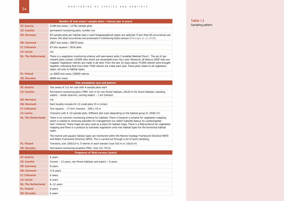
34M O N I T O R I N G O F S P E C I E S A N D H A B I T A T S
Table I.1 Sampling pattern
Number of test areas / sample plots / releves (per 6 years)
AT: Austria 3198 test areas / 12792 sample plots
CZ: Czechia permanent monitoring plots, number n/a
DE: Germany 63 sample plots per habitat type in each biogeographical region are selected. If less than 63 occurrences are known, the total occurrences are processed in monitoring (total census) (Ellwanger et. al, 2018).
DK: Denmark 2807 test areas / 28070 plots
LT: Lithuania 67 test squares / 1816 plots
LV: Latvia n/a
NL: The Netherlands There is a vegetation monitoring scheme with permanent plots (‘Landelijk Meetnet Flora’) . The set of per-manent plots contain 10,000 sites which are resampled every four year. Moreover, all Natura 2000 sites are mapped. Vegetation relevés are made in all sites. From the last 10 years about 75,000 relevés were brought together, indicating that more than 7500 relevés are made each year. These plots relate to all vegetation types, not only to habitat types.
PL: Poland ca. 6000 test areas /18000 releves
SK: Slovakia 6668 test areas
Test areas/plots size and pattern
AT: Austria Test areas of 1x1 km size with 4 sample plots each
CZ: Czechia Permanent monitoring plots (TMP), 5x5 m for non-forest habitats, 20x20 m for forest habitats, standing waters – whole reservoir, running waters – 1 km transect
DE: Germany n/a
DK: Denmark Each locality includes 8–12 small plots (5 m circles)
LT: Lithuania Test squares – 17 km2, transect – 200 x 10 m
LV: Latvia Transects with 3–10 sample plots. Different plot sizes depending on the habitat group (5–2500 m2)
NL: The Netherlands There is no common monitoring scheme for habitats. There is however a scheme for vegetation mapping which is related to receiving subsidies for management (so called ‘Subsidie Natuur en Landschapsbe-heer’-scheme). These maps are also used as a basis for habitat maps. There is a field protocol for vegetation mapping and there is a protocol to translate vegetation units into habitat types for the terrestrial habitat types.
The marine and aquatic habitat types are monitored within the Marine Strategy Framework Directive MSFD and Water Framework Directive (WFD). This is carried out through a set of point sampling.
PL: Poland Transects, size: 200x10 m; 3 releves in each transect (size 5x5 m or 10x10 m)
SK: Slovakia Permanent monitoring localities (PML). Size: 0,5–70 ha
Frequency of field surveys (years)
AT: Austria 6 years
CZ: Czechia Forests – 12 years, non-forest habitats and waters – 6 years
DE: Germany 6 years
DK: Denmark 3–6 years
LT: Lithuania 6 years
LV: Latvia 6 years
NL: The Netherlands 6–12 years
PL: Poland 6 years
SK: Slovakia 6 years
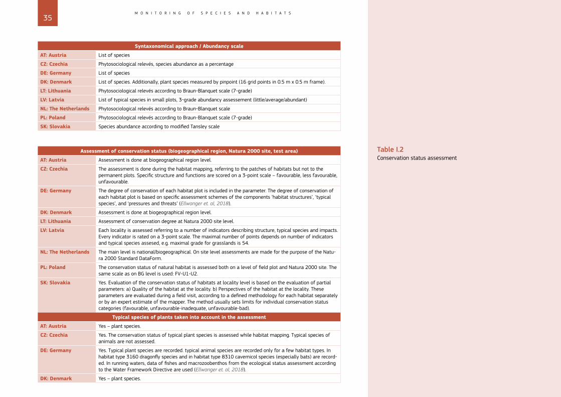
35M O N I T O R I N G O F S P E C I E S A N D H A B I T A T S
Syntaxonomical approach / Abundancy scale
AT: Austria List of species
CZ: Czechia Phytosociological relevés, species abundance as a percentage
DE: Germany List of species
DK: Denmark List of species. Additionally, plant species measured by pinpoint (16 grid points in 0.5 m x 0.5 m frame).
LT: Lithuania Phytosociological relevés according to Braun-Blanquet scale (7-grade)
LV: Latvia List of typical species in small plots, 3-grade abundancy assessement (little/average/abundant)
NL: The Netherlands Phytosociological relevés according to Braun-Blanquet scale
PL: Poland Phytosociological relevés according to Braun-Blanquet scale (7-grade)
SK: Slovakia Species abundance according to modified Tansley scale
Table I.2 Conservation status assessment
Assessment of conservation status (biogeographical region, Natura 2000 site, test area)
AT: Austria Assessment is done at biogeographical region level.
CZ: Czechia The assessment is done during the habitat mapping, referring to the patches of habitats but not to the permanent plots. Specific structure and functions are scored on a 3-point scale – favourable, less favourable, unfavourable.
DE: Germany The degree of conservation of each habitat plot is included in the parameter. The degree of conservation of each habitat plot is based on specific assessment schemes of the components ‘habitat structures’, ‘typical species’, and ‘pressures and threats’ (Ellwanger et. al, 2018).
DK: Denmark Assessment is done at biogeographical region level.
LT: Lithuania Assessment of conservation degree at Natura 2000 site level.
LV: Latvia Each locality is assessed referring to a number of indicators describing structure, typical species and impacts. Every indicator is rated on a 3-point scale. The maximal number of points depends on number of indicators and typical species assesed, e.g. maximal grade for grasslands is 54.
NL: The Netherlands The main level is national/biogeographical. On site level assessments are made for the purpose of the Natu-ra 2000 Standard DataForm.
PL: Poland The conservation status of natural habitat is assessed both on a level of field plot and Natura 2000 site. The same scale as on BG level is used: FV-U1-U2.
SK: Slovakia Yes. Evaluation of the conservation status of habitats at locality level is based on the evaluation of partial parameters: a) Quality of the habitat at the locality. b) Perspectives of the habitat at the locality. These parameters are evaluated during a field visit, according to a defined methodology for each habitat separately or by an expert estimate of the mapper. The method usually sets limits for individual conservation status categories (favourable, unfavourable-inadequate, unfavourable-bad).
Typical species of plants taken into account in the assessment
AT: Austria Yes – plant species.
CZ: Czechia Yes. The conservation status of typical plant species is assessed while habitat mapping. Typical species of animals are not assessed.
DE: Germany Yes. Typical plant species are recorded. typical animal species are recorded only for a few habitat types. In habitat type 3160 dragonfly species and in habitat type 8310 cavernicol species (especially bats) are record-ed. In running waters, data of fishes and macrozoobenthos from the ecological status assessment according to the Water Framework Directive are used (Ellwanger et. al, 2018).
DK: Denmark Yes – plant species.
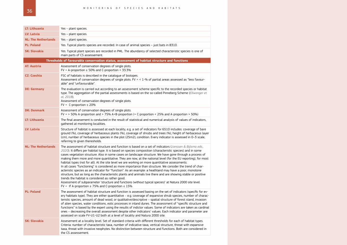
36M O N I T O R I N G O F S P E C I E S A N D H A B I T A T S
LT: Lithuania Yes – plant species.
LV: Latvia Yes – plant species.
NL: The Netherlands Yes – plant species.
PL: Poland Yes. Typical plants species are recorded. In case of animal species – just bats in 8310.
SK: Slovakia Yes. Typical plant species are recorded in PML. The abundancy of selected characteristic species is one of main parts of CS assessement.
Thresholds of favourable conservation status, assessment of habitat structure and functions
AT: Austria Assessment of conservation degrees of single plots. FV = A-proportion ≥ 50% and C-proportion < 33.3%
CZ: Czechia FSC of habitats is described in the catalogue of biotopes.Assessment of conservation degrees of single plots. FV = < 1-% of partial areas assessed as “less favour-able” and “unfavourable”.
DE: Germany The evaluation is carried out according to an assessment scheme specific to the recorded species or habitat type. The aggregation of the partial assessments is based on the so-called Pinneberg Scheme (Ellwanger et. al, 2018).Assessment of conservation degrees of single plots. FV = C-proportion ≤ 20%
DK: Denmark Assessment of conservation degrees of single plots.FV = > 50% A-proportion and > 75% A+B-proportion (= C-proportion < 25% and A-proportion > 50%)
LT: Lithuania The final assesement is conducted in the result of statistical and numerical analysis of values of indicators, gathered at monitoring localities.
LV: Latvia Structure of habitat is assessed at each locality, e.g. a set of indicators for 6510 includes: coverage of bare ground (%), coverage of herbaceous plants (%), coverage of shrubs and trees (%), height of herbaceous layer (cm), number of herbaceous species in the plot (25m2), condition. Every indicator is assessed in 0–3 scale, referring to given theresholds.
NL: The Netherlands The assessment of habitat structure and function is based on a set of indicators (Janssen & Bijlsma eds., 2020). It differs per habitat type. It is based on species composition (characteristic species) and in some cases vegetation structure. Also in some cases on landscape structure. We have gone through a process of making them more and more quantitative. They are now, at the national level (for the EU reporting), for most habitat types (not for all). At the site level we are working on more quantitative assessments.In all cases “functioning” is considered as more importance than structure. We consider the trend of char-acteristic species as an indicator for “function”. As an example: a heathland may have a poor, monotone structure, but as long as the characteristic plants and animals live there and are showing stable or positive trends the habitat is considered as rather good. Assessment of subparameter ‘structure and functions (without typical species)’ at Natura 2000 site level.FV = If A-proportion ≥ 75% and C-proportion ≤ 15%
PL: Poland The assessment of habitat structure and function is assessed basing on the set of indicators (specific for ev-ery habitats type). They are either quantitative – e.g. coverage of expansive shrub species, number of charac-teristic species, amount of dead wood, or qualitative/descriptive – spatial structure of forest stand, invasion of alien species, water conditions, eolic processes in inland dunes. The assessment of “specific structure and functions” is based by the expert using the results of indictor values. Some of indicators are taken as cardinal ones – decreasing the overall assessment despite other indicators’ values. Each indicator and parameter are assessed on scale FV-U1-U2 both at a level of locality and Natura 2000 site.
SK: Slovakia Assesement at a locality level. Set of standard criteria with different thresholds for each of habitat types. Criteria: number of characteristic taxa, number of indicative taxa, vertical structure, threat with expansive taxa, threat with invasive neophytes. No distinction between structure and functions. Both are considered in the CS assessement.
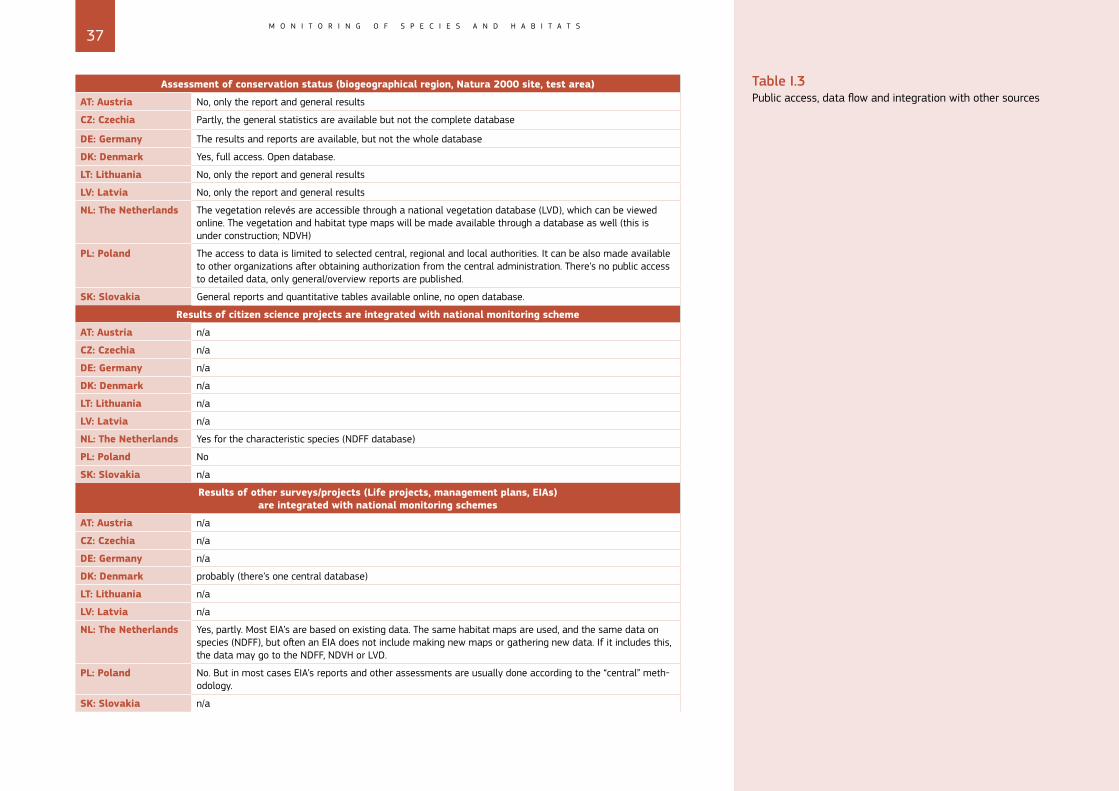
37M O N I T O R I N G O F S P E C I E S A N D H A B I T A T S
Table I.3 Public access, data flow and integration with other sources
Assessment of conservation status (biogeographical region, Natura 2000 site, test area)
AT: Austria No, only the report and general results
CZ: Czechia Partly, the general statistics are available but not the complete database
DE: Germany The results and reports are available, but not the whole database
DK: Denmark Yes, full access. Open database.
LT: Lithuania No, only the report and general results
LV: Latvia No, only the report and general results
NL: The Netherlands The vegetation relevés are accessible through a national vegetation database (LVD), which can be viewed online. The vegetation and habitat type maps will be made available through a database as well (this is under construction; NDVH)
PL: Poland The access to data is limited to selected central, regional and local authorities. It can be also made available to other organizations after obtaining authorization from the central administration. There’s no public access to detailed data, only general/overview reports are published.
SK: Slovakia General reports and quantitative tables available online, no open database.
Results of citizen science projects are integrated with national monitoring scheme
AT: Austria n/a
CZ: Czechia n/a
DE: Germany n/a
DK: Denmark n/a
LT: Lithuania n/a
LV: Latvia n/a
NL: The Netherlands Yes for the characteristic species (NDFF database)
PL: Poland No
SK: Slovakia n/a
Results of other surveys/projects (Life projects, management plans, EIAs) are integrated with national monitoring schemes
AT: Austria n/a
CZ: Czechia n/a
DE: Germany n/a
DK: Denmark probably (there’s one central database)
LT: Lithuania n/a
LV: Latvia n/a
NL: The Netherlands Yes, partly. Most EIA’s are based on existing data. The same habitat maps are used, and the same data on species (NDFF), but often an EIA does not include making new maps or gathering new data. If it includes this, the data may go to the NDFF, NDVH or LVD.
PL: Poland No. But in most cases EIA’s reports and other assessments are usually done according to the “central” meth-odology.
SK: Slovakia n/a
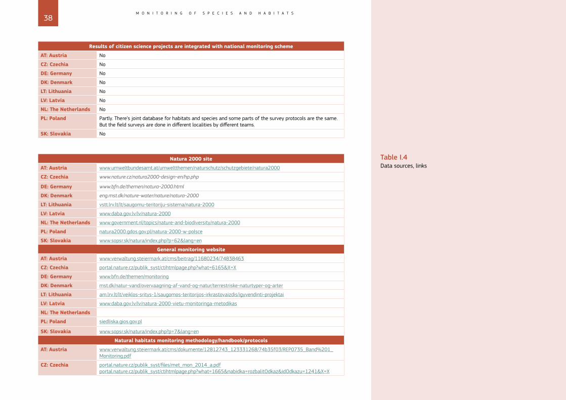
38M O N I T O R I N G O F S P E C I E S A N D H A B I T A T S
Results of citizen science projects are integrated with national monitoring scheme
AT: Austria No
CZ: Czechia No
DE: Germany No
DK: Denmark No
LT: Lithuania No
LV: Latvia No
NL: The Netherlands No
PL: Poland Partly. There’s joint database for habitats and species and some parts of the survey protocols are the same. But the field surveys are done in different localities by different teams.
SK: Slovakia No
Table I.4 Data sources, links
Natura 2000 site
AT: Austria www.umweltbundesamt.at/umweltthemen/naturschutz/schutzgebiete/natura2000
CZ: Czechia www.nature.cz/natura2000-design-en/hp.php
DE: Germany www.bfn.de/themen/natura-2000.html
DK: Denmark eng.mst.dk/nature-water/nature/natura-2000
LT: Lithuania vstt.lrv.lt/lt/saugomu-teritoriju-sistema/natura-2000
LV: Latvia www.daba.gov.lv/lv/natura-2000
NL: The Netherlands www.government.nl/topics/nature-and-biodiversity/natura-2000
PL: Poland natura2000.gdos.gov.pl/natura-2000-w-polsce
SK: Slovakia www.sopsr.sk/natura/index.php?p=62&lang=en
General monitoring website
AT: Austria www.verwaltung.steiermark.at/cms/beitrag/11680234/74838463
CZ: Czechia portal.nature.cz/publik_syst/ctihtmlpage.php?what=6165&X=X
DE: Germany www.bfn.de/themen/monitoring
DK: Denmark mst.dk/natur-vand/overvaagning-af-vand-og-natur/terrestriske-naturtyper-og-arter
LT: Lithuania am.lrv.lt/lt/veiklos-sritys-1/saugomos-teritorijos-irkrastovaizdis/igyvendinti-projektai
LV: Latvia www.daba.gov.lv/lv/natura-2000-vietu-monitoringa-metodikas
NL: The Netherlands
PL: Poland siedliska.gios.gov.pl
SK: Slovakia www.sopsr.sk/natura/index.php?p=7&lang=en
Natural habitats monitoring methodology/handbook/protocols
AT: Austria www.verwaltung.steiermark.at/cms/dokumente/12812743_123331268/74b35f03/REP0735_Band%201_Monitoring.pdf
CZ: Czechia portal.nature.cz/publik_syst/files/met_mon_2014_a.pdfportal.nature.cz/publik_syst/ctihtmlpage.php?what=1665&nabidka=rozbalitOdkaz&idOdkazu=1241&X=X
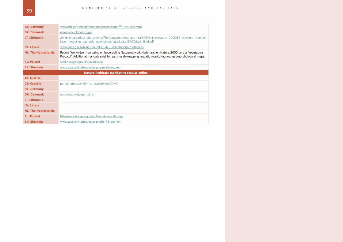
39M O N I T O R I N G O F S P E C I E S A N D H A B I T A T S
DE: Germany www.bfn.de/themen/monitoring/monitoring-ffh-richtlinie.html
DK: Denmark novana.au.dk/naturtyper
LT: Lithuania am.lrv.lt/uploads/am/documents/files/saugom_teritorijos_kra%C5%A1tov/natura_2000/EB_buveiniu_monitor-ingo_metodiniu_pagrindu_parengimas_ataskaita_II%20dalis_final.pdf
LV: Latvia www.daba.gov.lv/lv/natura-2000-vietu-monitoringa-metodikas
NL: The Netherlands Report ‘Werkwijze monitoring en beoordeling Natuurnetwerk Nederland en Natura 2000’ and a ‘Vegetation Protocol’. Additional manuals exist for salt marsh-mapping, aquatic monitoring and geomorphological maps.
PL: Poland siedliska.gios.gov.pl/pl/publikacje
SK: Slovakia www.sopsr.sk/natura/index.php?p=7&lang=en
Natural habitats monitoring results online
AT: Austria
CZ: Czechia portal.nature.cz/nd/x_nd_statistiky.php?X=X
DE: Germany
DK: Denmark naturdata.miljoeportal.dk
LT: Lithuania
LV: Latvia
NL: The Netherlands
PL: Poland http://siedliska.gios.gov.pl/pl/wyniki-monitoringu
SK: Slovakia www.sopsr.sk/natura/index.php?p=7&lang=en