Copyright © 2011 by The McGraw-Hill Companies, Inc. All rights reserved.McGraw-Hill/Irwin

Chapter FifteenChapter FifteenIndependent Demand InventoryIndependent Demand Inventory

Operations ManagementOperations ManagementContemporary Concepts and Cases 5/eContemporary Concepts and Cases 5/e

15-2

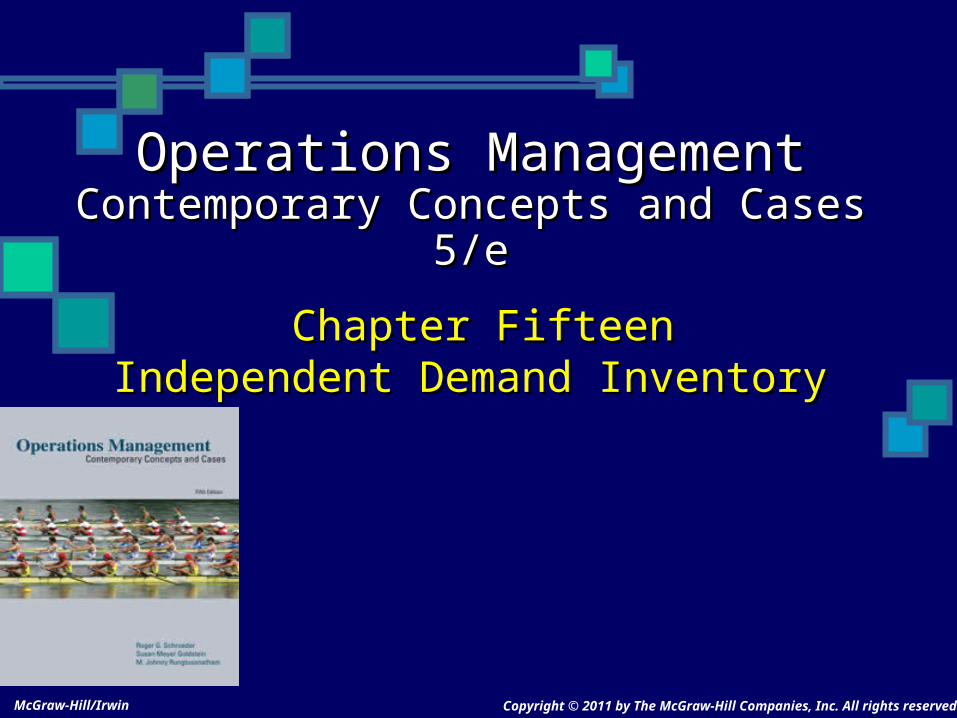
Chapter 15 OutlineChapter 15 Outline

Purpose of InventoriesPurpose of Inventories

Costs of InventoriesCosts of Inventories

Independent versus Dependent DemandIndependent versus Dependent Demand

Economic Order QuantityEconomic Order Quantity

Continuous Review SystemContinuous Review System

Periodic Review SystemPeriodic Review System

Using P and Q System in PracticeUsing P and Q System in Practice

ABC Inventory ManagementABC Inventory Management

15-3

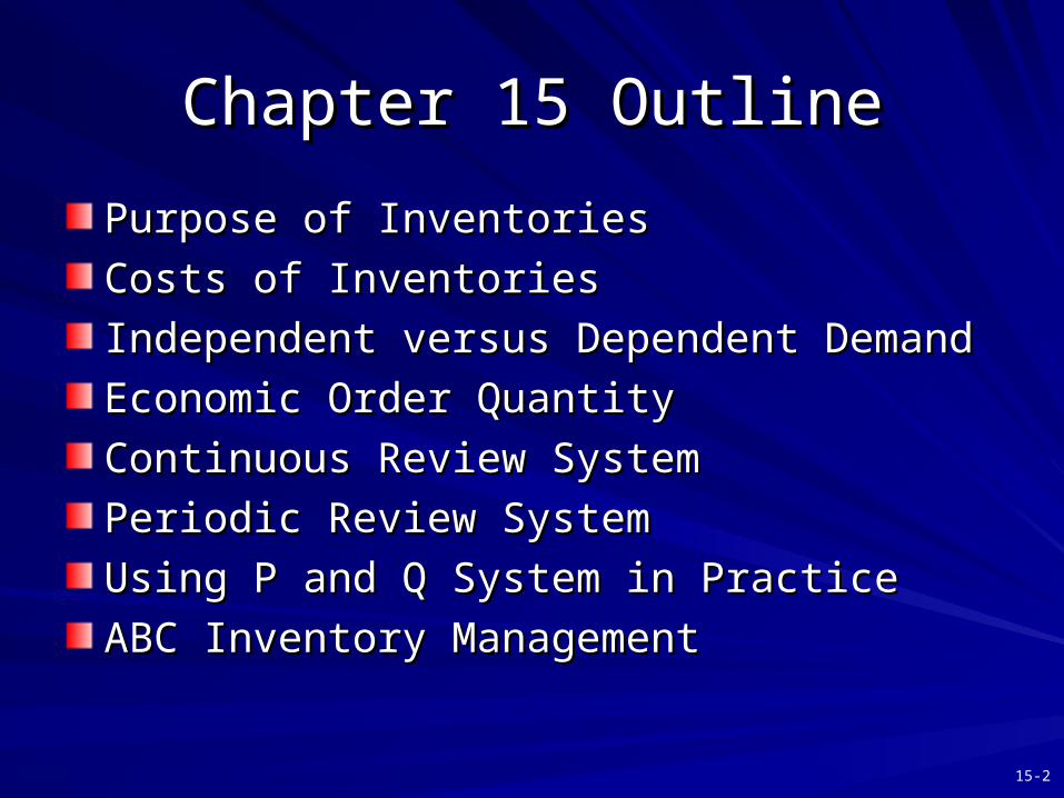
DefinitionsDefinitions

Inventory: a stock of materials used to facilitate Inventory: a stock of materials used to facilitate production or satisfy customer demandproduction or satisfy customer demand

Types of inventoryTypes of inventory– Raw materials, purchased parts (RM)Raw materials, purchased parts (RM)– Work in process (WIP)Work in process (WIP)– Finished goods (FG)Finished goods (FG)– Maintenance, repair & operating supplies (MRO)Maintenance, repair & operating supplies (MRO)

15-4

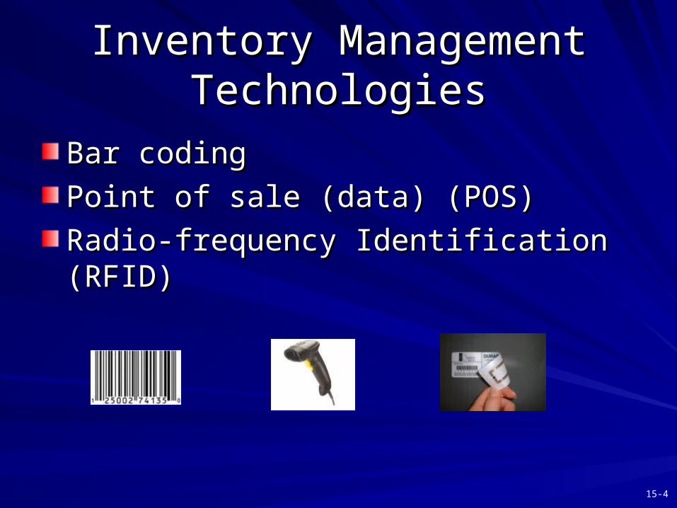
Inventory Management Inventory Management TechnologiesTechnologies

Bar codingBar coding

Point of sale (data) (POS)Point of sale (data) (POS)

Radio-frequency Identification (RFID) Radio-frequency Identification (RFID)

15-5

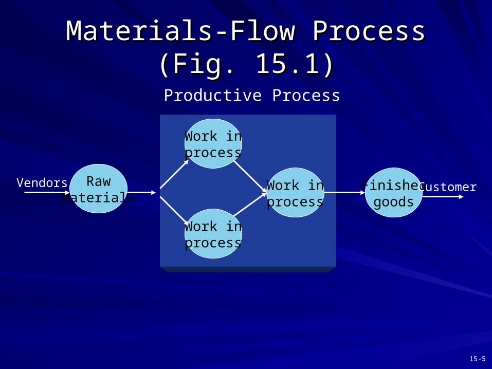
Materials-Flow Process (Fig. 15.1)Materials-Flow Process (Fig. 15.1)

Work inprocess

Work inprocess

Work inprocess

Finishedgoods

RawMaterials

Vendors Customer

Productive Process

15-6

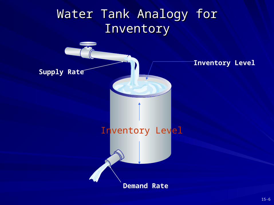
Water Tank Analogy for InventoryWater Tank Analogy for Inventory

Supply RateInventory Level

Demand Rate

Inventory Level

15-7

Purpose of Inventories (1)Purpose of Inventories (1)

To protect against To protect against uncertaintiesuncertainties (safety stock) (safety stock)– demand (FG, MRO)demand (FG, MRO)– supply (RM, MRO)supply (RM, MRO)– lead times (RM, WIP)lead times (RM, WIP)– schedule changes (WIP)schedule changes (WIP)

To allow economic production and purchase To allow economic production and purchase (discounts for buying RM in bulk)(discounts for buying RM in bulk)

15-8

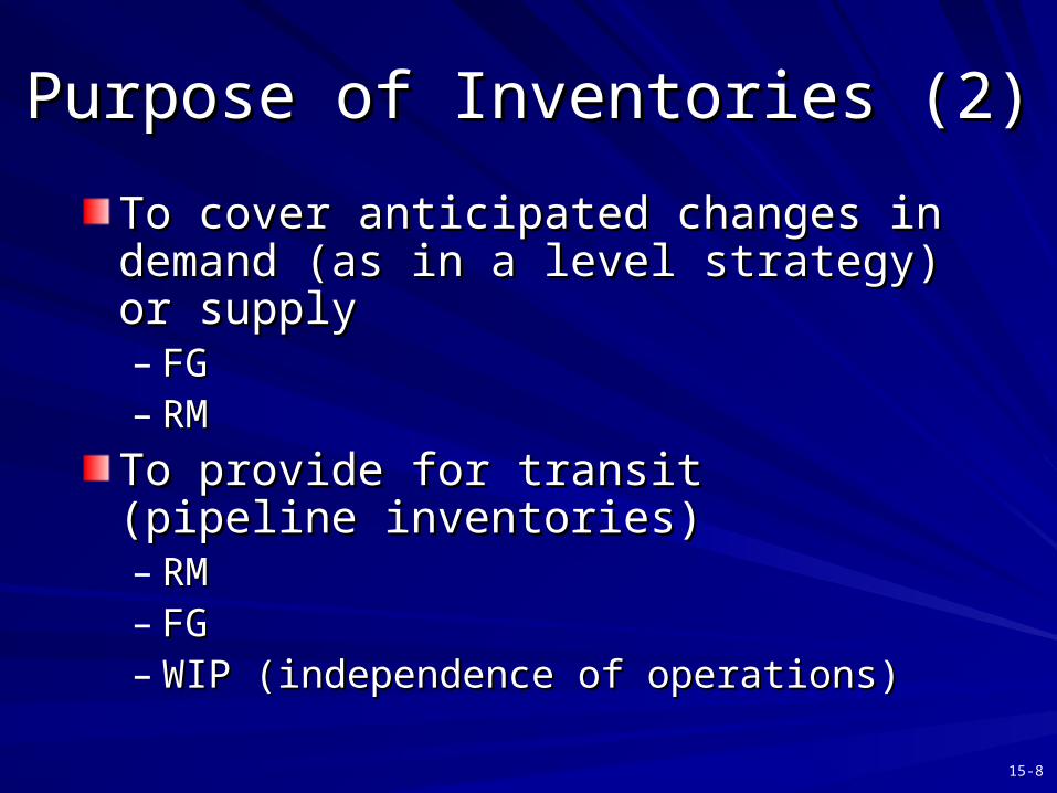
Purpose of Inventories (2)Purpose of Inventories (2)

To cover anticipated changes in demand (as To cover anticipated changes in demand (as in a level strategy) or supplyin a level strategy) or supply– FGFG– RMRM

To provide for transit (pipeline inventories)To provide for transit (pipeline inventories)– RMRM– FGFG– WIP (independence of operations)WIP (independence of operations)

15-9

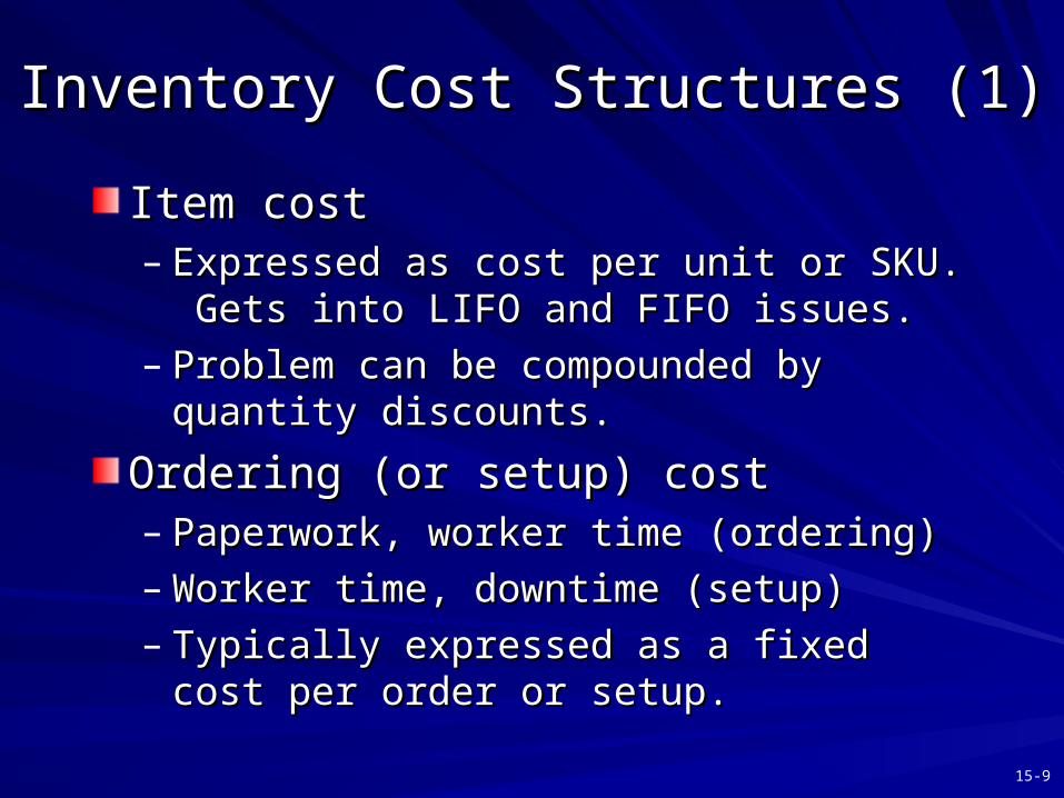
Inventory Cost Structures (Inventory Cost Structures (11))

Item costItem cost– Expressed as cost per unit or SKU. Gets into Expressed as cost per unit or SKU. Gets into

LIFO and FIFO issues. LIFO and FIFO issues. – Problem can be compounded by quantity Problem can be compounded by quantity

discounts.discounts.

Ordering (or setup) costOrdering (or setup) cost– Paperwork, worker time (ordering)Paperwork, worker time (ordering)– Worker time, downtime (setup)Worker time, downtime (setup)– Typically expressed as a fixed cost per order or Typically expressed as a fixed cost per order or

setup. setup.

15-10

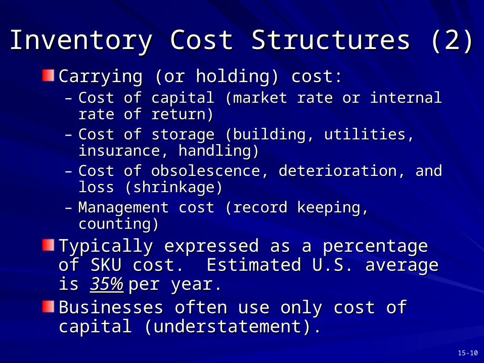
Inventory Cost Structures (2)Inventory Cost Structures (2)Carrying (or holding) cost:Carrying (or holding) cost:– Cost of capital (market rate or internal rate of return)Cost of capital (market rate or internal rate of return)– Cost of storage (building, utilities, insurance, handling)Cost of storage (building, utilities, insurance, handling)– Cost of obsolescence, deterioration, and loss Cost of obsolescence, deterioration, and loss

(shrinkage)(shrinkage)– Management cost (record keeping, counting)Management cost (record keeping, counting)

Typically expressed as a percentage of SKU cost. Typically expressed as a percentage of SKU cost. Estimated U.S. average is Estimated U.S. average is 35%35% per year.per year.Businesses often use only cost of capital Businesses often use only cost of capital (understatement).(understatement).

15-11

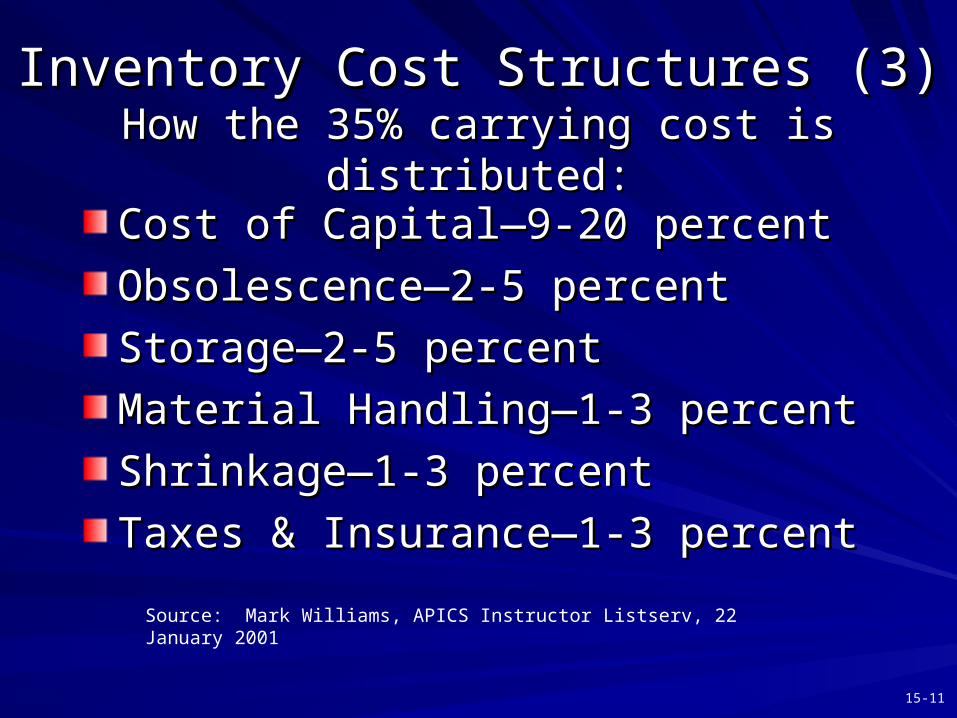
Inventory Cost Structures (3)Inventory Cost Structures (3)How the 35% carrying cost is distributed:How the 35% carrying cost is distributed:

Cost of Capital—9-20 percentCost of Capital—9-20 percent

Obsolescence—2-5 percentObsolescence—2-5 percent

Storage—2-5 percentStorage—2-5 percent

Material Handling—1-3 percentMaterial Handling—1-3 percent

Shrinkage—1-3 percentShrinkage—1-3 percent

Taxes & Insurance—1-3 percentTaxes & Insurance—1-3 percent

Source: Mark Williams, APICS Instructor Listserv, 22 January 2001

15-12

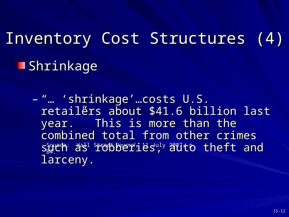
Inventory Cost Structures (4)Inventory Cost Structures (4)

ShrinkageShrinkage

– “… ‘“… ‘shrinkage’…costs U.S. retailers about $41.6 shrinkage’…costs U.S. retailers about $41.6 billion last year.” This is more than the combined billion last year.” This is more than the combined total from other crimes such as robberies, auto total from other crimes such as robberies, auto theft and larceny.theft and larceny.

Source: Wall Street Journal, 11 July 2007, p. B4.

15-13

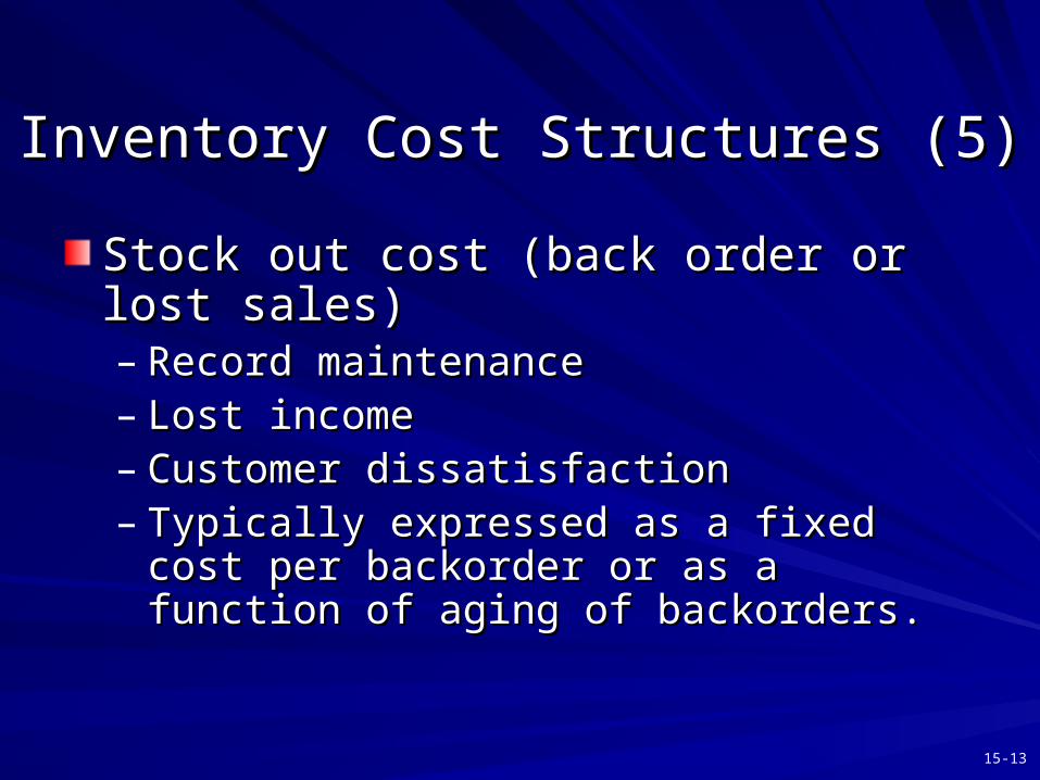
Inventory Cost Structures (5)Inventory Cost Structures (5)

Stock out cost (back order or lost sales)Stock out cost (back order or lost sales)– Record maintenanceRecord maintenance– Lost incomeLost income– Customer dissatisfactionCustomer dissatisfaction– Typically expressed as a fixed cost per backorder Typically expressed as a fixed cost per backorder

or as a function of aging of backorders.or as a function of aging of backorders.

15-14

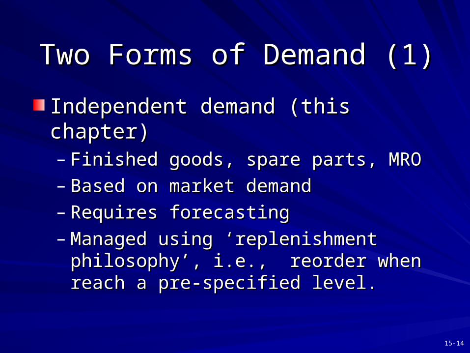
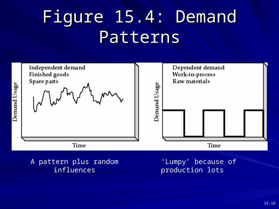
Two Forms of Demand (1)Two Forms of Demand (1)

Independent demandIndependent demand (this chapter)(this chapter)– Finished goods, spare parts, MROFinished goods, spare parts, MRO– Based on market demandBased on market demand– Requires forecastingRequires forecasting– Managed using ‘replenishment philosophy’, i.e., Managed using ‘replenishment philosophy’, i.e.,

reorder when reach a pre-specified level.reorder when reach a pre-specified level.

15-15

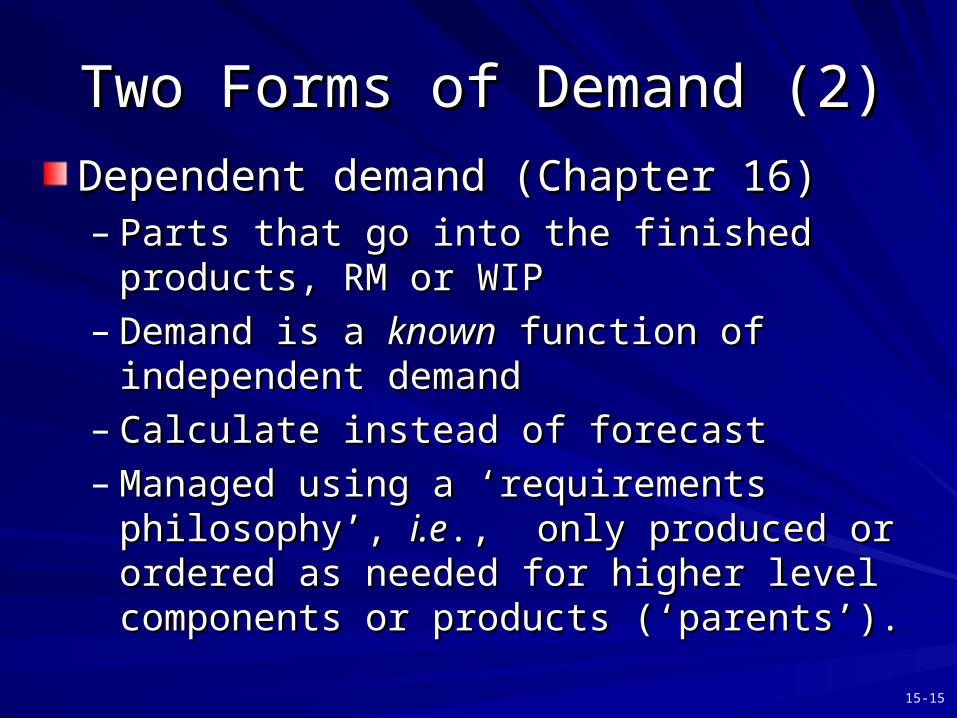
Two Forms of Demand (2)Two Forms of Demand (2)

Dependent demandDependent demand (Chapter 16)(Chapter 16)– Parts that go into the finished products, RM orParts that go into the finished products, RM or WIPWIP– Demand is a Demand is a knownknown function of independent demand function of independent demand– Calculate instead of forecastCalculate instead of forecast– Managed using a ‘requirements philosophy’, Managed using a ‘requirements philosophy’, i.ei.e., .,

only produced or ordered as needed for higher level only produced or ordered as needed for higher level components or products (‘parents’).components or products (‘parents’).

15-16

Figure 15.4: Demand PatternsFigure 15.4: Demand Patterns

A pattern plus random influences ‘Lumpy’ because of production lots

15-17

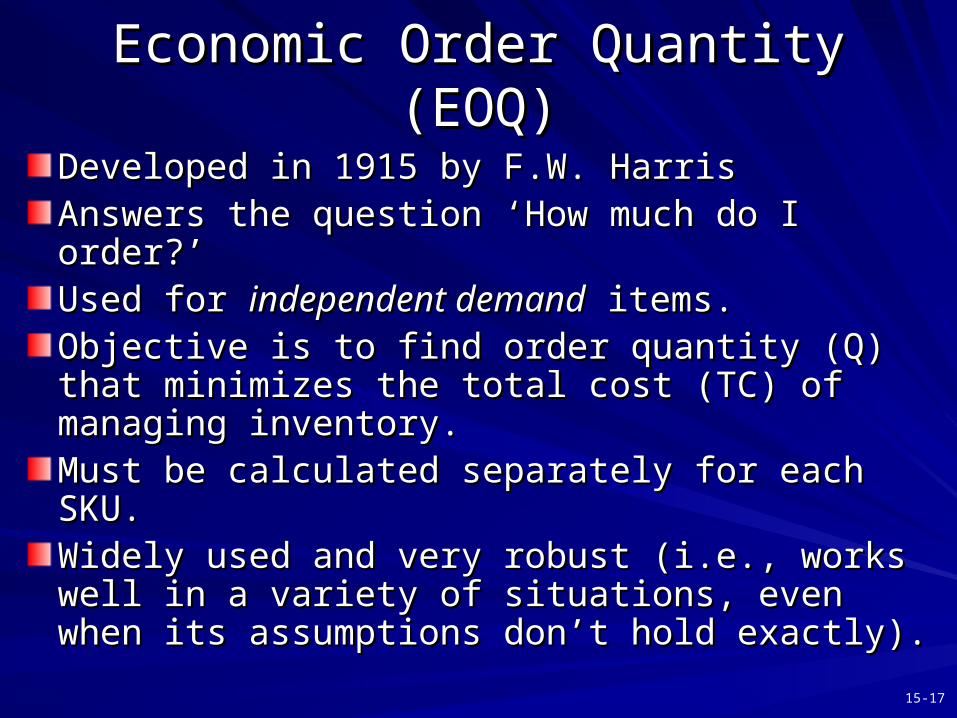
Economic Order Quantity (EOQ)Economic Order Quantity (EOQ)

Developed in 1915 by F.W. HarrisDeveloped in 1915 by F.W. HarrisAnswers the question ‘How much do I order?’Answers the question ‘How much do I order?’Used for Used for independent demandindependent demand items. items.Objective is to find order quantity (Q) that minimizes Objective is to find order quantity (Q) that minimizes the total cost (TC) of managing inventory.the total cost (TC) of managing inventory.Must be calculated separately for each SKU.Must be calculated separately for each SKU.Widely used and very robust (i.e., works well in a Widely used and very robust (i.e., works well in a variety of situations, even when its assumptions don’t variety of situations, even when its assumptions don’t hold exactly). hold exactly).

15-18

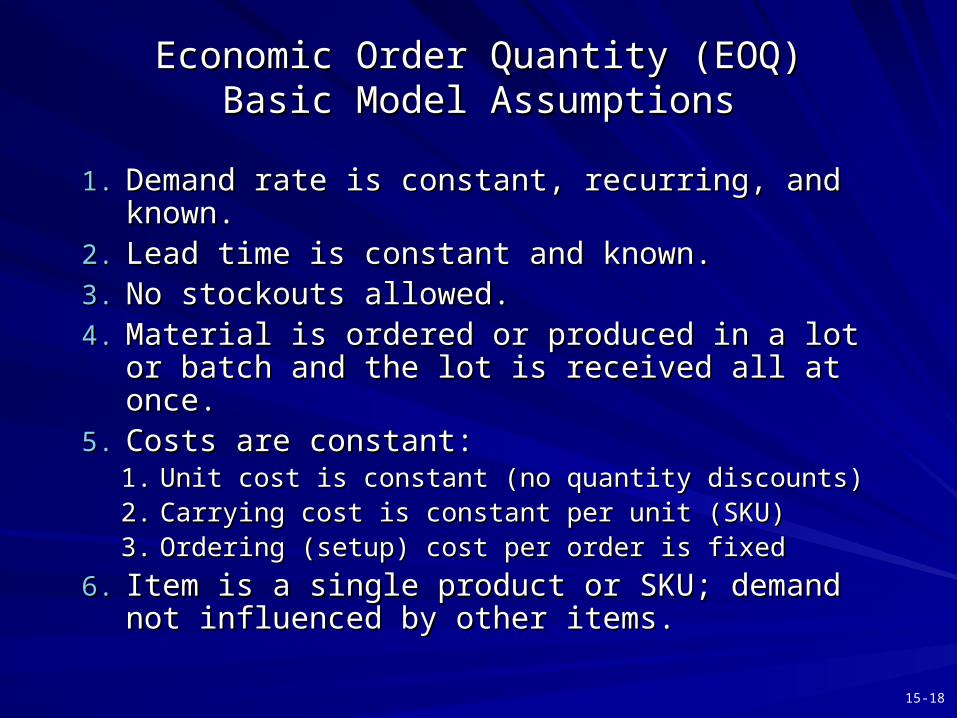
Economic Order Quantity (EOQ)Economic Order Quantity (EOQ)Basic Model AssumptionsBasic Model Assumptions

1.1. Demand rate is constant, recurring, and known.Demand rate is constant, recurring, and known.2.2. Lead time is constant and known.Lead time is constant and known.3.3. No stockouts allowed.No stockouts allowed.4.4. Material is ordered or produced in a lot or batch Material is ordered or produced in a lot or batch

and the lot is received all at once.and the lot is received all at once.5.5. Costs are constant:Costs are constant:

1.1. Unit cost is constant (no quantity discounts)Unit cost is constant (no quantity discounts)2.2. Carrying cost is constant per unit (SKU)Carrying cost is constant per unit (SKU)3.3. Ordering (setup) cost per order is fixedOrdering (setup) cost per order is fixed

6.6. Item is a single product or SKU; demand not Item is a single product or SKU; demand not influenced by other items.influenced by other items.

15-19

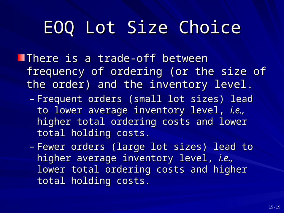
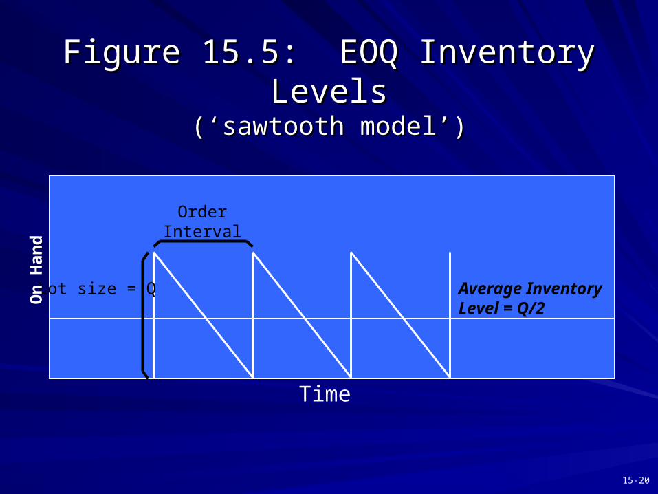
EOQ Lot Size ChoiceEOQ Lot Size Choice

There is a trade-off between frequency of There is a trade-off between frequency of ordering (or the size of the order) and the ordering (or the size of the order) and the inventory level.inventory level.– Frequent orders (small lot sizes) lead to lower Frequent orders (small lot sizes) lead to lower

average inventory level, average inventory level, i.e.,i.e., higher total ordering higher total ordering costs and lower total holding costs.costs and lower total holding costs.

– Fewer orders (large lot sizes) lead to higher Fewer orders (large lot sizes) lead to higher average inventory level, average inventory level, i.e.,i.e., lower total ordering lower total ordering costs and higher total holding costs.costs and higher total holding costs.

15-20

Figure 15.5: EOQ Inventory LevelsFigure 15.5: EOQ Inventory Levels(‘sawtooth model’)(‘sawtooth model’)

Time

Lot size = Q

OrderInterval

Average InventoryLevel = Q/2

On

Han

d

15-21

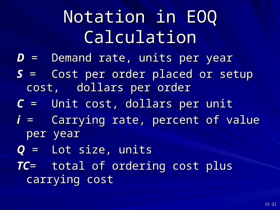
Notation in EOQ CalculationNotation in EOQ Calculation

DD = = Demand rate, units per yearDemand rate, units per year

SS = = Cost per order placed or setup cost,Cost per order placed or setup cost,dollars per orderdollars per order

CC = = Unit cost, dollars per unitUnit cost, dollars per unit

ii = = Carrying rate, percent of value per yearCarrying rate, percent of value per year

QQ = = Lot size, unitsLot size, units

TCTC== total of ordering cost plus carrying costtotal of ordering cost plus carrying cost

15-22

Cost Equations in EOQCost Equations in EOQ

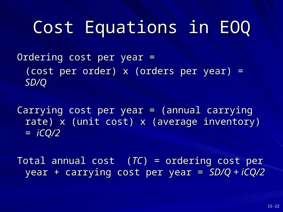
Ordering cost per year = Ordering cost per year =

(cost per order) x (orders per year) = (cost per order) x (orders per year) = SD/QSD/Q

Carrying cost per year = (annual carrying rate) x Carrying cost per year = (annual carrying rate) x (unit cost) x (average inventory) = (unit cost) x (average inventory) = iCQ/2iCQ/2

Total annual cost (Total annual cost (TCTC) = ordering cost per year ) = ordering cost per year + carrying cost per year = + carrying cost per year = SD/Q + iCQ/2SD/Q + iCQ/2

15-23

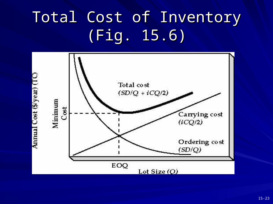
Total Cost of Inventory (Fig. 15.6)Total Cost of Inventory (Fig. 15.6)

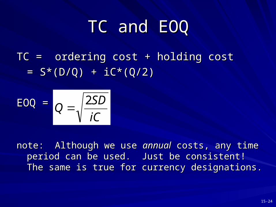
TC and EOQTC and EOQ

TC = ordering cost + holding cost TC = ordering cost + holding cost

= S*(D/Q) + iC*(Q/2) = S*(D/Q) + iC*(Q/2)

EOQ =EOQ =

note: Although we use note: Although we use annualannual costs, any time period can be used. costs, any time period can be used. Just be consistent! The same is true for currency designations.Just be consistent! The same is true for currency designations.

iC

SDQ

2

15-24

15-25

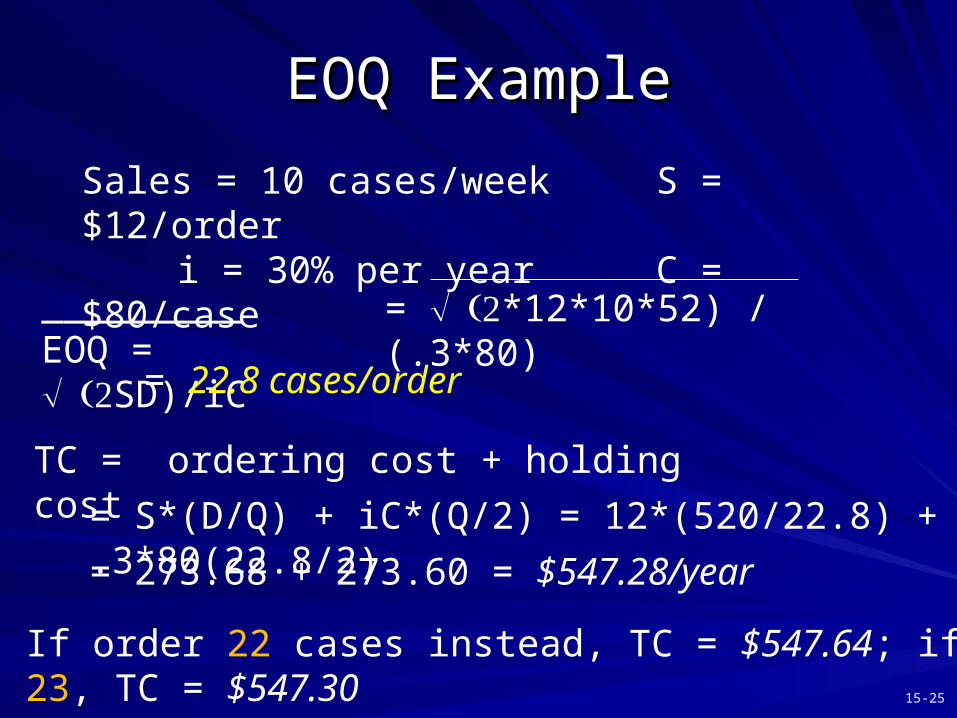
EOQ ExampleEOQ Example

Sales = 10 cases/week S = $12/orderi = 30% per year C = $80/case

_________EOQ = SD)/iC = *12*10*52) / (.3*80)

= 22.8 cases/order

TC = ordering cost + holding cost

= S*(D/Q) + iC*(Q/2) = 12*(520/22.8) + .3*80(22.8/2)

= 273.68 + 273.60 = $547.28/year

If order 22 cases instead, TC = $547.64; if 23, TC = $547.30

15-26

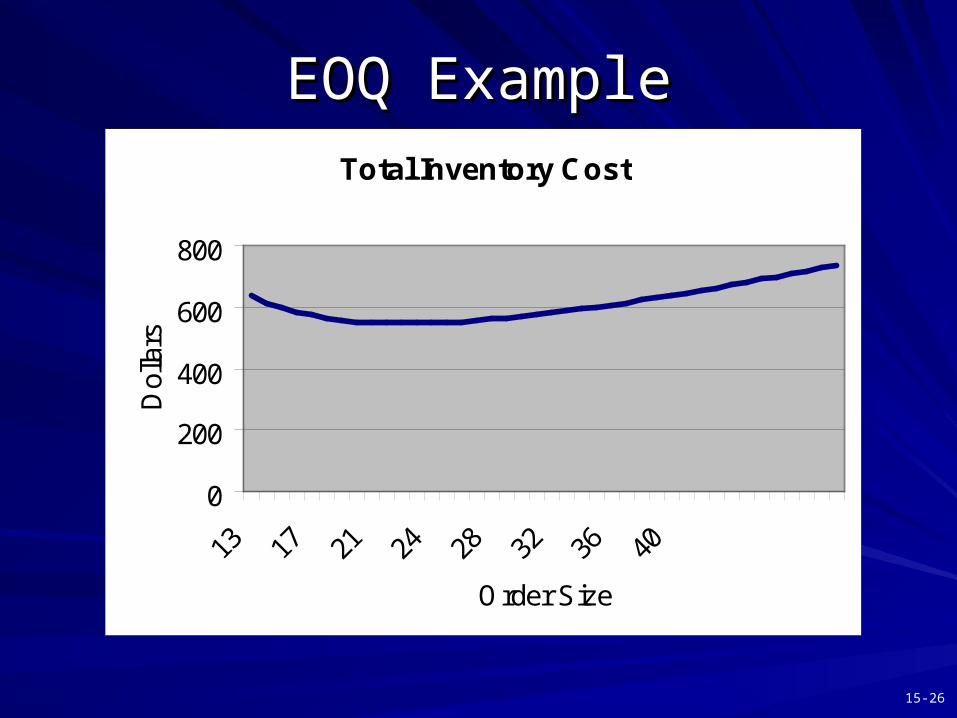
EOQ ExampleEOQ ExampleTotal Inventory Cost

0

200

400

600

800

13 17 21 24 28 32 36 40

Order Size

Dol

lars

15-27

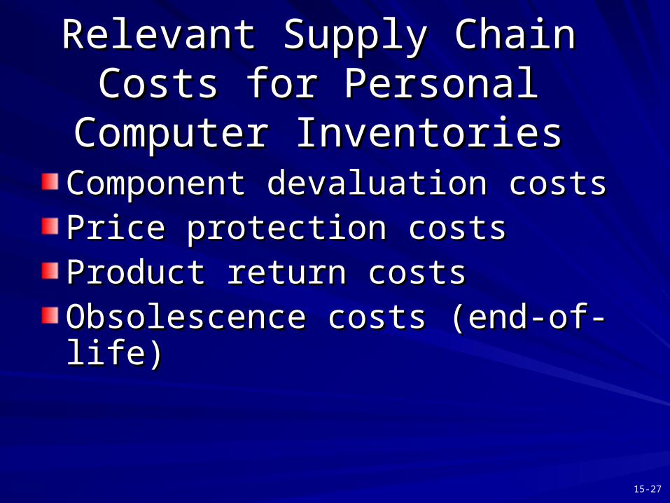
Relevant Supply Chain Costs for Relevant Supply Chain Costs for Personal Computer InventoriesPersonal Computer Inventories

Component devaluation costsComponent devaluation costsPrice protection costsPrice protection costsProduct return costsProduct return costsObsolescence costs (end-of-life)Obsolescence costs (end-of-life)

15-28

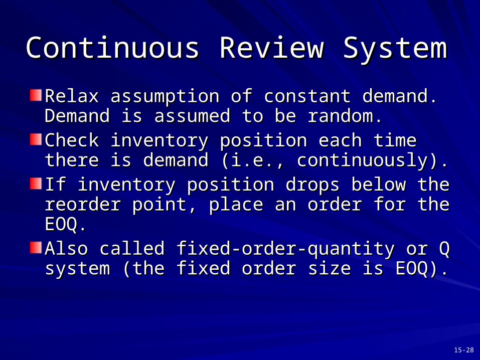
Continuous Review SystemContinuous Review System

Relax assumption of constant demand. Relax assumption of constant demand. Demand is assumed to be random.Demand is assumed to be random.Check inventory position each time there is Check inventory position each time there is demand (i.e., continuously).demand (i.e., continuously).If inventory position drops below the reorder If inventory position drops below the reorder point, place an order for the EOQ.point, place an order for the EOQ.Also called fixed-order-quantity or Q system Also called fixed-order-quantity or Q system (the fixed order size is EOQ).(the fixed order size is EOQ).

15-29

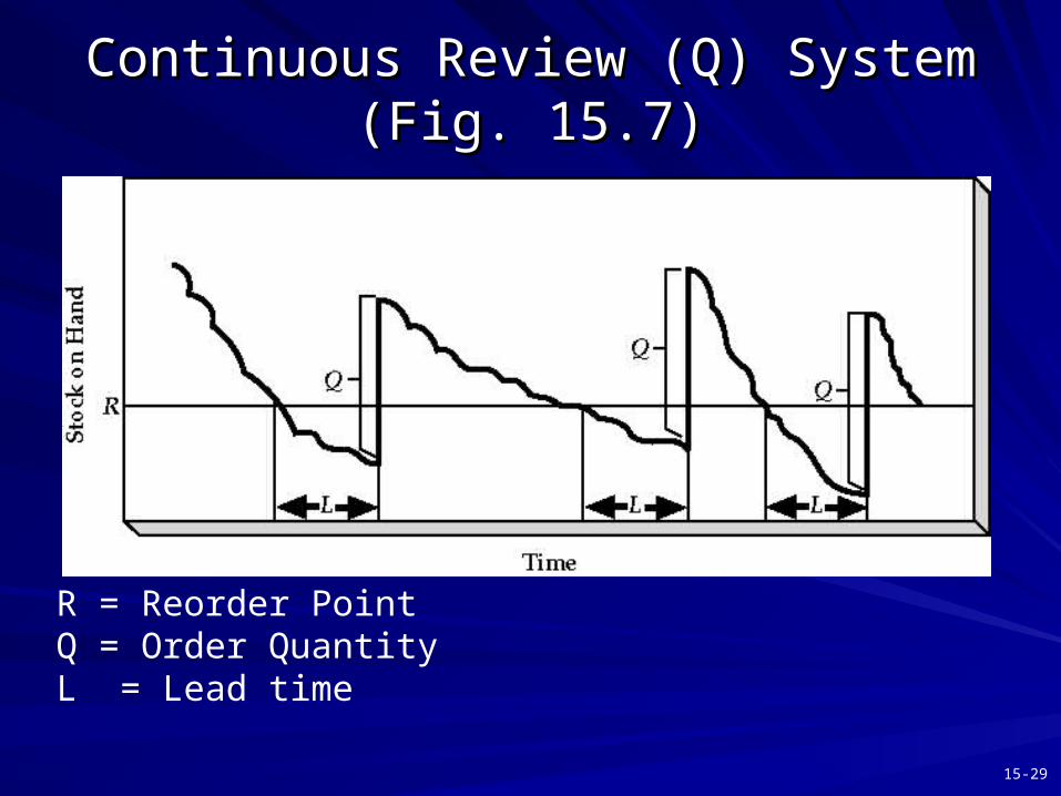
Continuous Review (Q) System (Fig. 15.7)Continuous Review (Q) System (Fig. 15.7)

R = Reorder PointQ = Order QuantityL = Lead time

15-30

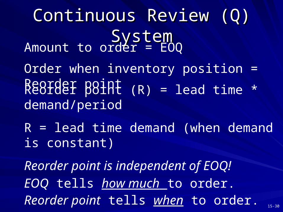
Continuous Review (Q) SystemContinuous Review (Q) SystemAmount to order = EOQ

Order when inventory position = Reorder point

Reorder point (R) = lead time * demand/period

R = lead time demand (when demand is constant)

Reorder point is independent of EOQ!

EOQ tells how much to order.Reorder point tells when to order.

15-31

Service LevelService Level

When demand is random, the reorder point When demand is random, the reorder point must take into account the desired service must take into account the desired service level or fill rate.level or fill rate.

Service level has many definitions:Service level has many definitions:– Probability that all orders will be refilled while Probability that all orders will be refilled while

waiting for an order to arrive.waiting for an order to arrive.– Percentage of demand filled from stock in a time Percentage of demand filled from stock in a time

period.period.– Percentage of time the system has stock on hand.Percentage of time the system has stock on hand.

15-32

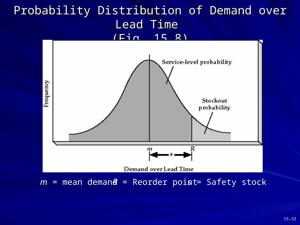
Probability Distribution of Demand over Lead Time Probability Distribution of Demand over Lead Time (Fig. 15.8)(Fig. 15.8)

m = mean demand R = Reorder point s = Safety stock

15-33

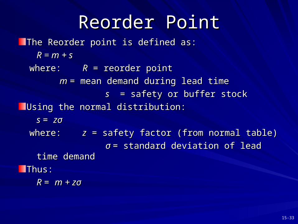
Reorder PointReorder PointThe Reorder point is defined as:The Reorder point is defined as:

R = m + sR = m + s

where:where: RR = reorder point = reorder point

m m = mean demand during lead time= mean demand during lead time

ss = safety or buffer stock = safety or buffer stock

Using the normal distribution:Using the normal distribution:

s s = = zzσσ

where: where: zz = safety factor (from normal table) = safety factor (from normal table)

σσ = standard deviation of lead time demand= standard deviation of lead time demand

Thus:Thus:

R R = = m + m + zzσσ

15-34

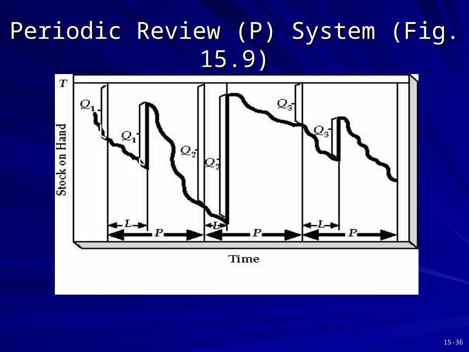
Periodic Review System (1)Periodic Review System (1)

Instead of reviewing continuously, we review Instead of reviewing continuously, we review the inventory position at the inventory position at fixed intervalsfixed intervals. For . For example, the bread truck visits the grocery example, the bread truck visits the grocery store on the same days every week.store on the same days every week.

Inventory brought up to a ‘target’ level.Inventory brought up to a ‘target’ level.

Also known as “P system,” “Fixed-order-Also known as “P system,” “Fixed-order-interval system” or “Fixed-order-period interval system” or “Fixed-order-period system”system”

15-35

Periodic Review System (2)Periodic Review System (2)

Has a target inventory level rather than a Has a target inventory level rather than a reorder point.reorder point.

Does not use EOQ (directly) since order Does not use EOQ (directly) since order quantity varies according to demand.quantity varies according to demand.

The order interval is The order interval is fixedfixed, the order quantity , the order quantity variesvaries..

15-36

Periodic Review (P) System (Fig. 15.9)Periodic Review (P) System (Fig. 15.9)

15-37

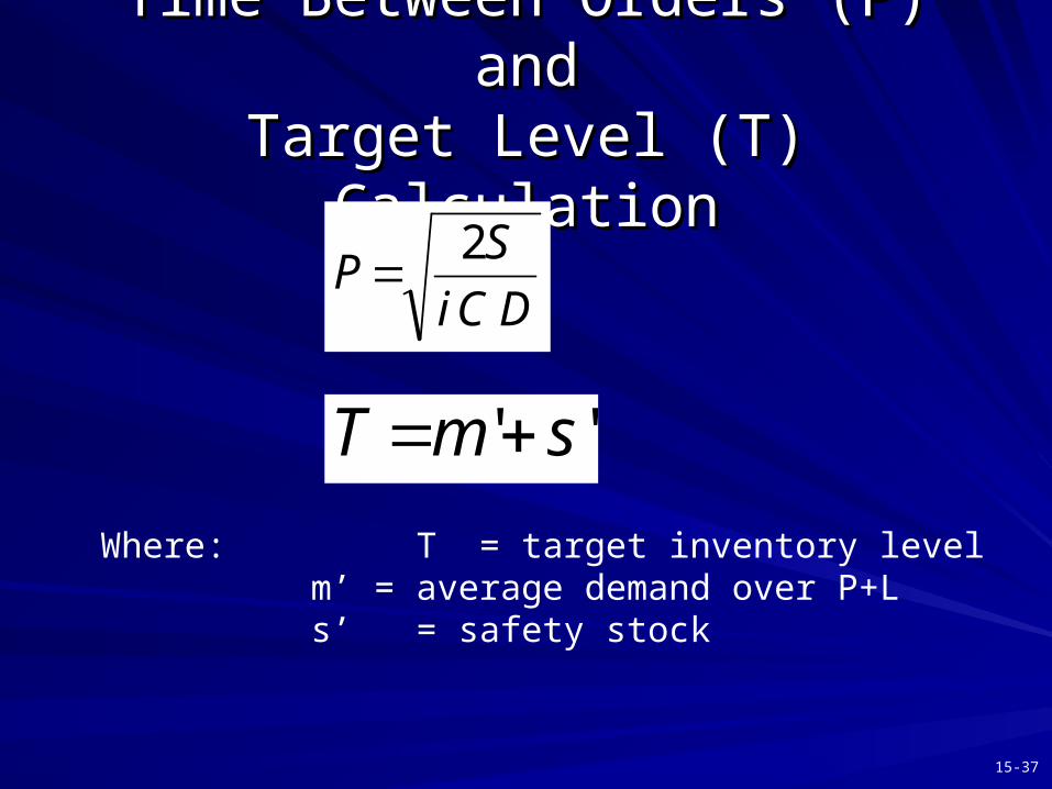
Time Between Orders (P) andTime Between Orders (P) andTarget Level (T) CalculationTarget Level (T) Calculation

DCi

SP

2

'' smT Where: T = target inventory level

m’ = average demand over P+Ls’ = safety stock

15-38

Using P and Q System in PracticeUsing P and Q System in Practice

Use P system when orders must be placed at Use P system when orders must be placed at specified intervals.specified intervals.

Use P systems when multiple items are Use P systems when multiple items are ordered from the same supplier (joint-ordered from the same supplier (joint-replenishment).replenishment).

Use P system for inexpensive items.Use P system for inexpensive items.

15-39

Using P and Q Systems in PracticeUsing P and Q Systems in Practice

P may be easier to use since levels are P may be easier to use since levels are reviewed less often.reviewed less often.

P requires more safety stock since may only P requires more safety stock since may only order at fixed points.order at fixed points.

P is more likely to run out since cannot P is more likely to run out since cannot respond quickly to increases in demand.respond quickly to increases in demand.

Either may be more costly: P in safety Either may be more costly: P in safety stock, Q in monitoring cost.stock, Q in monitoring cost.

15-40

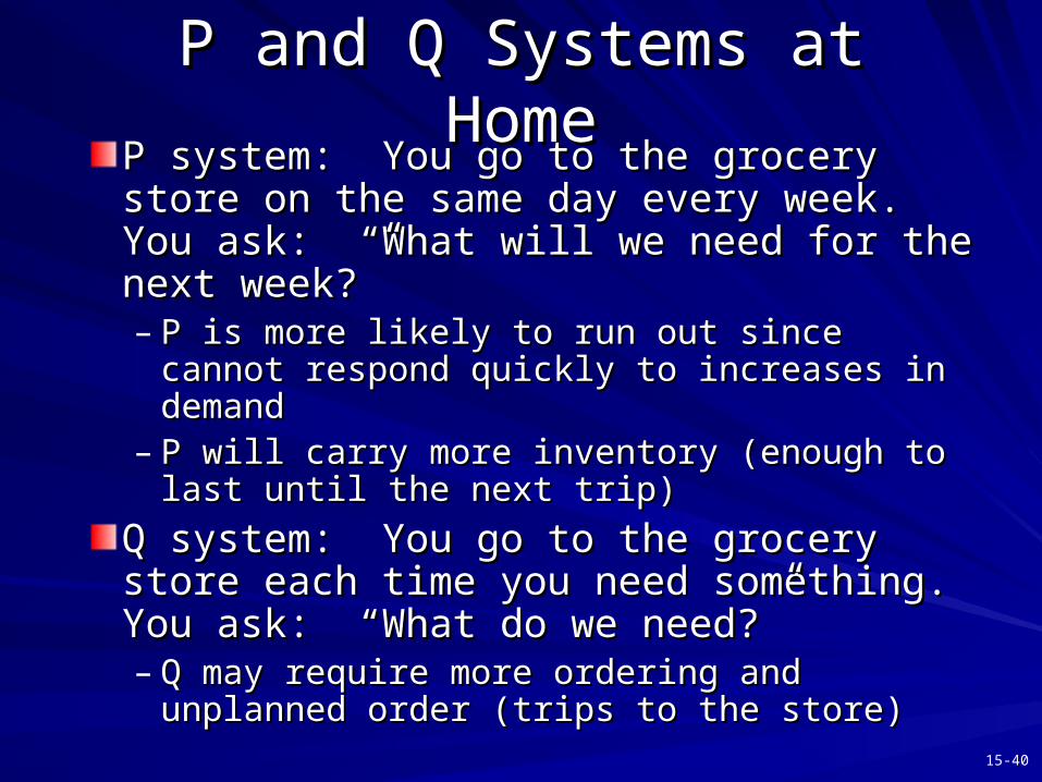
P and Q Systems at HomeP and Q Systems at HomeP system: You go to the grocery store on the P system: You go to the grocery store on the same day every week. You ask: “What will same day every week. You ask: “What will we need for the next week?”we need for the next week?”– P is more likely to run out since cannot respond P is more likely to run out since cannot respond

quickly to increases in demandquickly to increases in demand– P will carry more inventory (enough to last until P will carry more inventory (enough to last until

the next trip)the next trip)

Q system: You go to the grocery store each Q system: You go to the grocery store each time you need something. You ask: “What time you need something. You ask: “What do we need?”do we need?”– Q may require more ordering and unplanned Q may require more ordering and unplanned

order (trips to the store)order (trips to the store)

15-41

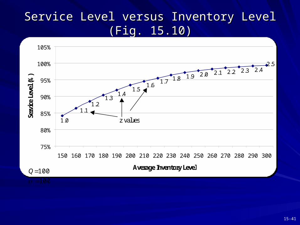
Service Level versus Inventory Level (Fig. 15.10)Service Level versus Inventory Level (Fig. 15.10)

1.1

2.52.42.32.22.12.01.91.81.7

1.61.5

1.31.2

1.0

1.4

75%

80%

85%

90%

95%

100%

105%

150 160 170 180 190 200 210 220 230 240 250 260 270 280 290 300

Average Inventory Level

Serv

ice Le

vel (

%)

z values

100

100

Q

15-42

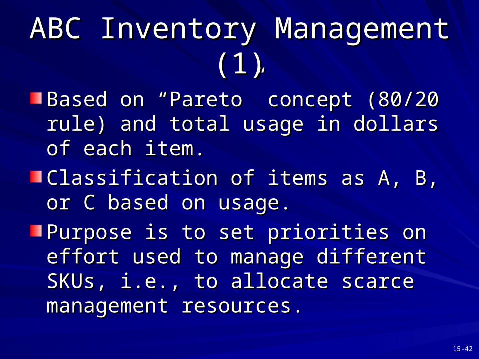
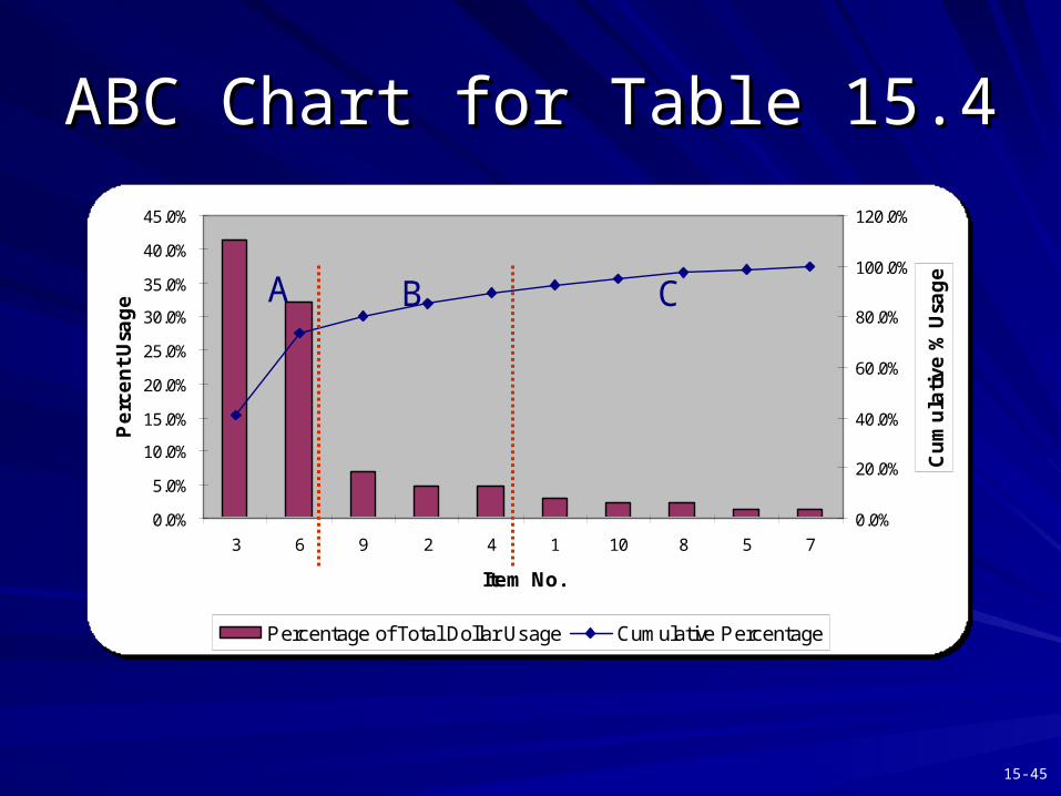
ABC Inventory Management (1)ABC Inventory Management (1)

Based on “Pareto” concept (80/20 rule) and Based on “Pareto” concept (80/20 rule) and total usage in dollars of each item.total usage in dollars of each item.

Classification of items as A, B, or C based on Classification of items as A, B, or C based on usage.usage.

Purpose is to set priorities on effort used to Purpose is to set priorities on effort used to manage different SKUs, i.e., to allocate scarce manage different SKUs, i.e., to allocate scarce management resources.management resources.

15-43

ABC Inventory Management (2)ABC Inventory Management (2)

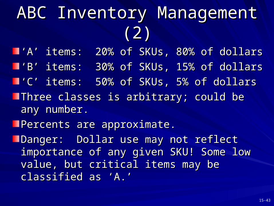
‘‘A’ items: 20% of SKUs, 80% of dollarsA’ items: 20% of SKUs, 80% of dollars

‘‘B’ items: 30% of SKUs, 15% of dollarsB’ items: 30% of SKUs, 15% of dollars

‘‘C’ items: 50% of SKUs, 5% of dollarsC’ items: 50% of SKUs, 5% of dollars

Three classes is arbitrary; could be any number.Three classes is arbitrary; could be any number.

Percents are approximate.Percents are approximate.

Danger: Dollar use may not reflect importance of Danger: Dollar use may not reflect importance of any given SKU! Some low value, but critical any given SKU! Some low value, but critical items may be classified as ‘A.’items may be classified as ‘A.’

15-44

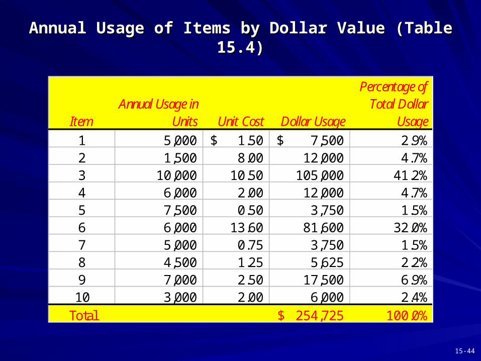
Annual Usage of Items by Dollar Value (Table 15.4)Annual Usage of Items by Dollar Value (Table 15.4)

ItemAnnual Usage in

Units Unit Cost Dollar Usage

Percentage of Total Dollar

Usage1 5,000 1.50$ 7,500$ 2.9%2 1,500 8.00 12,000 4.7%3 10,000 10.50 105,000 41.2%4 6,000 2.00 12,000 4.7%5 7,500 0.50 3,750 1.5%6 6,000 13.60 81,600 32.0%7 5,000 0.75 3,750 1.5%8 4,500 1.25 5,625 2.2%9 7,000 2.50 17,500 6.9%10 3,000 2.00 6,000 2.4%

Total 254,725$ 100.0%

15-45

ABC Chart for Table 15.4ABC Chart for Table 15.4

0.0%

5.0%

10.0%

15.0%

20.0%

25.0%

30.0%

35.0%

40.0%

45.0%

3 6 9 2 4 1 10 8 5 7

Item No.

Pe

rce

nt

Usa

ge

0.0%

20.0%

40.0%

60.0%

80.0%

100.0%

120.0%

Cu

mu

lati

ve %

Usa

ge

Percentage of Total Dollar Usage Cumulative Percentage

A B C

15-46

SummarySummaryPurpose of InventoriesPurpose of Inventories

Costs of InventoriesCosts of Inventories

Independent versus Dependent DemandIndependent versus Dependent Demand

Economic Order QuantityEconomic Order Quantity

Continuous Review SystemContinuous Review System

Periodic Review SystemPeriodic Review System

Using P and Q System in PracticeUsing P and Q System in Practice

ABC Inventory ManagementABC Inventory Management

15-47

End of Chapter Fifteen