HAL Id: insu-00196672https://hal-insu.archives-ouvertes.fr/insu-00196672

Submitted on 13 Dec 2007

HAL is a multi-disciplinary open accessarchive for the deposit and dissemination of sci-entific research documents, whether they are pub-lished or not. The documents may come fromteaching and research institutions in France orabroad, or from public or private research centers.

L’archive ouverte pluridisciplinaire HAL, estdestinée au dépôt et à la diffusion de documentsscientifiques de niveau recherche, publiés ou non,émanant des établissements d’enseignement et derecherche français ou étrangers, des laboratoirespublics ou privés.

Characterisation of soils with stony inclusions usinggeoelectrical measurements

Etienne Rey, Denis Jongmans, Philippe, Gotteland„ Stéphane Garambois

To cite this version:Etienne Rey, Denis Jongmans, Philippe, Gotteland„ Stéphane Garambois. Characterisation of soilswith stony inclusions using geoelectrical measurements. Journal of Applied Geophysics, Elsevier, 2006,58, pp.188-201. <10.1016/j.jappgeo.2005.06.003>. <insu-00196672>

CHARACTERISATION OF SOILS

WITH STONY INCLUSIONS USING GEOELECTRICAL

MEASUREMENTS

Etienne Rey, Denis Jongmans*,

Philippe Gotteland, Stephane Garambois

L.I.R.I.G.M., Grenoble University,

Maison des Géosciences, BP 53X, 38041 Grenoble Cedex 9, France

* Corresponding author :

Tel. :+0033-4 76 82 81 17 Fax : +0033-4 76 82 80 70.

E-mail adress : denis.jongmans@ujf-grenoble.fr

1

ABSTRACT

Characterisation and sampling of coarse heterogeneous soils is often impossible using common

geotechnical in-situ tests once the soil contains particles with a diameter larger than a few decimetres.

In this situation geophysical techniques - and particularly electrical measurements - can act as an

alternative method for obtaining information about the ground characteristics. This paper deals with

the use of electrical tomography on heterogeneous diphasic media consisting of resistive inclusions

embedded in a conductive matrix. The adopted approach articulates in three steps: numerical

modelling, measurements on a small-scale physical model, and field measurements. Electrical

measurements were simulated using finite element analyses, on a numerical model containing a

random concentration of inclusions varying from 0 to 40 %. It is shown that for electrode spacing 8

times greater than the radius of inclusions, the equivalent homogeneous resistivity is obtained. In this

condition, average measured resistivity is a function of the concentration of inclusions, in agreement

with the theoretical laws. To apply these results on real data, a small-scale physical model has been

built, where electrical measurements were conducted both on the model and on each phase. From

these laboratory measurements, a very satisfying estimation of the percentage of inclusions has been

obtained. Finally, the methodology applied to a real experimental site composed of alluvial fan

deposits made of limestone rocks embedded in a clayey matrix. The estimated percentage of rock

particles obtained via electrical measurements was in accordance with the real grain size distribution.

2

1 INTRODUCTION

Coarse soils such as scree-slopes, till, alluvial fans, debris flows or slope deposits are commonly

present in mountainous areas. The presence of decimetre to meter size pebbles or rocks in these

deposits makes them difficult to characterise using traditional geotechnical techniques. First, in-situ

tests like penetration tests or boreholes are hard to perform in such loose and heterogeneous

formations. Second, the presence of decimetric rocks would require an elementary representative

volume of soil (e.g. Standard NFP 94-056) much too large (several tens of cubic meters) for the

traditional soil test devices. These materials are generally characterised by a two-phases procedure

which consists in: (i) removing the grains larger than 100 millimetres in size and (ii) performing

geotechnical tests on the remaining soil. However, such a procedure results in an underestimate of

the mechanical characteristics of the geological formation. Indeed the angle of friction increases with

the maximum particle size (Fagnoul & Bonnechere, 1969; Bourdeau, 1997) and with the proportion

of grains, due to interlocking (Holtz, 1961). As classical geotechnical techniques are not efficient to

characterize coarse materials at a scale which is consistent with their maximum particle size,

alternative methods have to be developed, at least to estimate the overall proportion of grains, which

constitute an interesting information in terms of mechanical properties.

Geophysical methods, which are non-intrusive and able to investigate a large volume of soil, may

constitute an interesting alternative to in-situ geotechnical tests. Quick and relatively cheap to

perform, they are able to characterise coarse formations as a whole and to detect lateral variations of

geophysical properties (P-wave velocity, S-wave velocity, electrical resistivity…). Their main

drawbacks are the decrease of the resolution with depth and that mechanical properties of the soil

3

are not directly accessed. However, empirical correlations between geophysical and geotechnical

parameters have been proposed, particularly between shear wave velocity and strength properties

(e.g., Mayne & Rix, 1995).

One of the main geophysical methods for deriving shear wave velocity profiles is the inversion of

surface waves (Jongmans & Demanet, 1993). Several attempts were made to apply this method

when characterising heterogeneous materials or “hard-to-sample” soils (Stockoe et al., 1988).

Recently, Chammas et al. (2003) showed that Rayleigh waves are well-suited to the determination of

shear wave velocity of a heterogeneous soil layer. Indeed, for wavelengths 7.5 times greater than the

radius of circular inclusions, and within a concentration range from 0 to 50 %, surface waves

homogenize the soil in accordance with the multiple-scattering homogenization theory (Christensen &

Lo, 1979). By simulating via finite-element analysis, several random distributions of inclusions made

of limestone or sandstone in a sandy matrix, Chammas et al. (2003) evinced the increase of the shear

wave velocity Vs with the concentration of stiff inclusions (for velocity contrasts ranging from 2.4 to

5.5). This relationship, validated using a small-scale model (Abraham et al., 2004) at two different

concentrations (19% and 35%), allows one to estimate the concentration of inclusions present in a

soil using only seismic measurement techniques.

Electrical resistivity (or conductivity), which is an easy geophysical parameter to measure in the field,

exhibits a wide range of values in nature, from 1 Ωm in clay or contaminated soil to more than 104

Ωm in rocks like limestone or granite (Reynolds, 1997). Even if electrical and mechanical properties

of the soils are not directly linked, electrical resistivity of a material is sensitive to the presence of

resistive or conductive inclusions. For the interpretation of borehole resistivity logs in porous rocks,

4

many authors studied the link between the effective resistivity (macroscopic, with regard to the size

of heterogeneities) of the saturated porous rocks and its characteristics (porosity, fluid

conductivity…). Many decades ago, Archie (1942) performed DC electrical measurements on

brine-saturated cores for a wide variety of sand formations and proposed a simple empirical

relationship (equation 1) between the effective (equivalent homogeneous) resistivity ρ0 of the rock,

the resistivity of the fluid ρf, the cementation factor m and the porosity φ.

m

f

F −== φρρ0 . (1)

The ratio F is called the formation factor. According to Archie, m varies from 1.3 for unconsolidated

sands to 1.8 to 2 for consolidated sandstones. From their electrical measurements on unconsolidated

marine sands obeying to Archie’s law, Jackson et al. (1978) concluded that exponent m is entirely

dependent upon the shape of the resistive particles, varying from 1.2 for spheres to 1.9 for platey

shell fragments. A possible explanation for these variations is that the m exponent value increases

when the conduction paths are more tortuous (Jackson et al., 1978). By performing measurements

on artificial porous rocks obtained by the fusion of glass beads, Sen et al (1981) attributed a value of

1.5 to the cementation factor in accordance with their homogenisation model. Geometrical

considerations conducted Mendelson and Cohen (1982) to demonstrate that m takes a value of 1.5

for spherical rock particles spread in three dimensions, in accordance with the results of Sen et al.

(1981). Cementation factor m takes on a value of 2 in the case of cylinders with their axes

perpendicular to electrical field (Sen et al., 1981) and for circular grains in two dimensions

(Mendelson & Cohen, 1982). In these Differential Effective Medium approaches, the desired

concentration of inclusions is reached by adding infinitesimal increments of dispersed inclusions to a

5

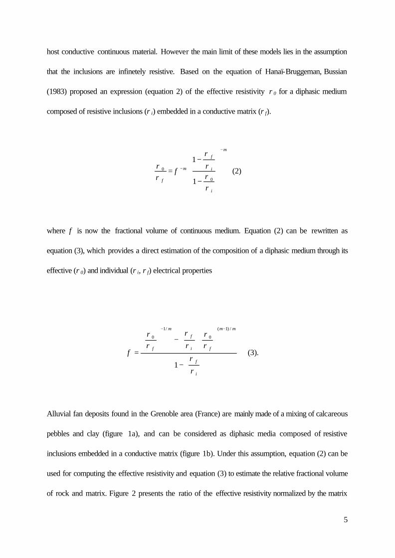
host conductive continuous material. However the main limit of these models lies in the assumption

that the inclusions are infinetely resistive. Based on the equation of Hanaï-Bruggeman, Bussian

(1983) proposed an expression (equation 2) of the effective resistivity ρ0 for a diphasic medium

composed of resistive inclusions (ρi) embedded in a conductive matrix (ρf).

m

i

i

f

m

f

−

−

−

−=

ρρρ

ρ

φρρ

0

0

1

1 (2)

where φ is now the fractional volume of continuous medium. Equation (2) can be rewritten as

equation (3), which provides a direct estimation of the composition of a diphasic medium through its

effective (ρ0) and individual (ρi, ρf) electrical properties

−

−

=

−−

i

f

mm

fi

f

m

f

ρ

ρ

ρρ

ρ

ρ

ρρ

φ

1

/)1(

0

/1

0

(3).

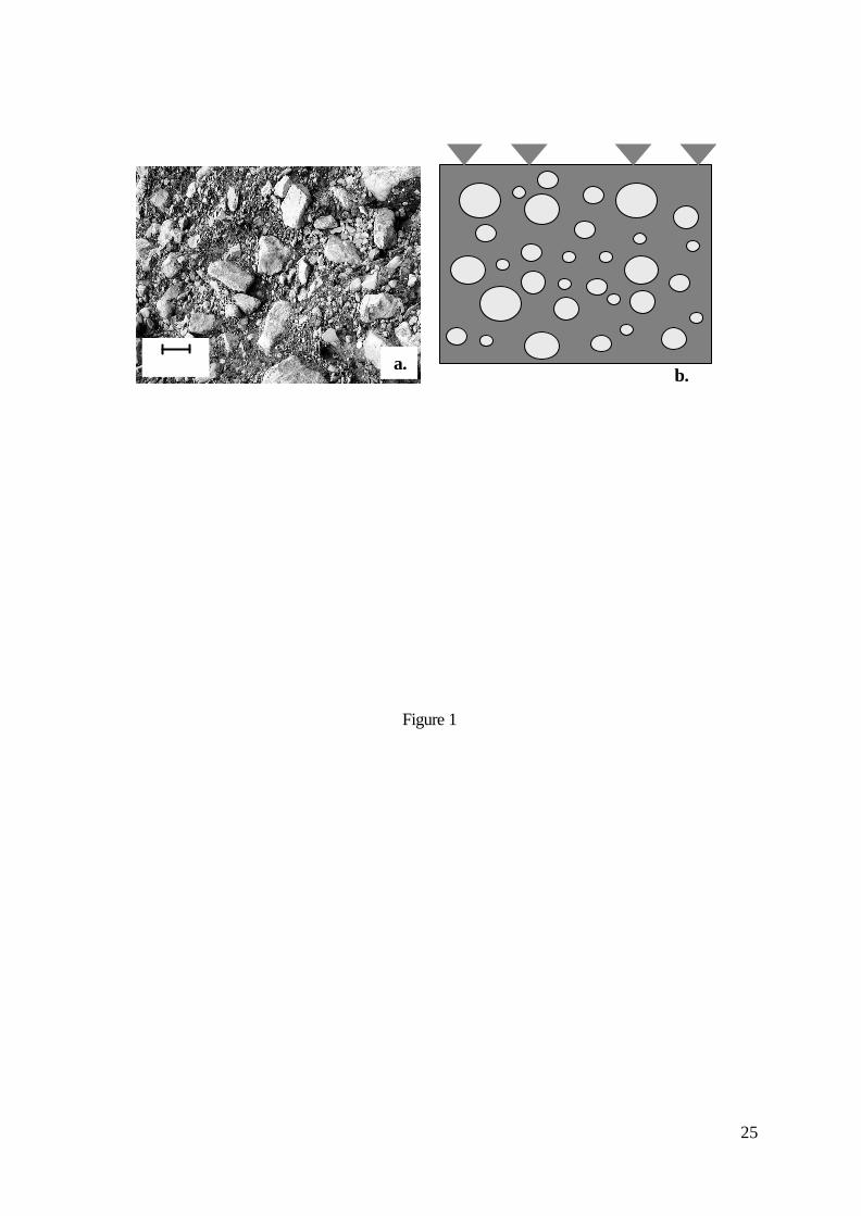
Alluvial fan deposits found in the Grenoble area (France) are mainly made of a mixing of calcareous

pebbles and clay (figure 1a), and can be considered as diphasic media composed of resistive

inclusions embedded in a conductive matrix (figure 1b). Under this assumption, equation (2) can be

used for computing the effective resistivity and equation (3) to estimate the relative fractional volume

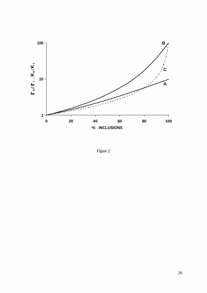
of rock and matrix. Figure 2 presents the ratio of the effective resistivity normalized by the matrix

6

value (ρ0 /ρf) as a function of the percentage of inclusions, for 2 different contrasts of resistivity

between matrix and inclusions (ρi /ρf = 10 and 100) and for m=2. On the same graph is plotted the

homogenisation curve of the bulk modulus (Christensen & Lo, 1979) for a shear wave velocity

contrast of 10. For the same contrast value, the electrical effective resistivity appears more sensitive

to the presence of inclusions than the effective bulk modulus until an inclusion percentage of 80%.

Insofar as electrical properties of natural materials vary in a wider range than the seismic ones, the

electrical tomography technique seems to be a promising method to investigate heterogeneous soils

where resistive particles are present.

This paper proposes a methodology to estimate the composition of coarse heterogeneous soils using

electrical measurements. Our approach articulates in three steps. The first step involves the use of

finite element analysis (F.E.A.) to simulate electrical tomography experiments on a diphasic soil with

known characteristics. The objective was to specify the required conditions for homogenizing the soil

resistivity and to compare the numerical results with the predictions of the theoretical laws. In the

second step, these requirements were tested using measurements performed on a small-scale

laboratory model, where the concentration of resistive inclusions was known. In the last step, the

methodology was applied to a real experimental site, where grain size analyses were performed on

several samples in order to verify the predictions derived from electrical and electromagnetic

measurements.

2 NUMERICAL MODELLING OF ELECTRICAL TOMOGRAPHY

7

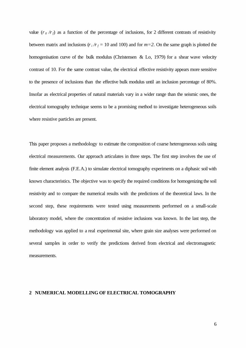
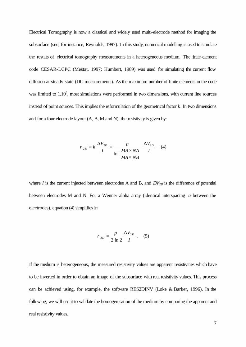
Electrical Tomography is now a classical and widely used multi-electrode method for imaging the

subsurface (see, for instance, Reynolds, 1997). In this study, numerical modelling is used to simulate

the results of electrical tomography measurements in a heterogeneous medium. The finite-element

code CESAR-LCPC (Mestat, 1997; Humbert, 1989) was used for simulating the current flow

diffusion at steady state (DC measurements). As the maximum number of finite elements in the code

was limited to 1.105, most simulations were performed in two dimensions, with current line sources

instead of point sources. This implies the reformulation of the geometrical factor k. In two dimensions

and for a four electrode layout (A, B, M and N), the resistivity is given by:

IV

NBMANAMBI

Vk DD

D22

2

ln

∆

××

=∆

=π

ρ (4)

where I is the current injected between electrodes A and B, and ∆V2D is the difference of potential

between electrodes M and N. For a Wenner alpha array (identical interspacing a between the

electrodes), equation (4) simplifies in:

IV D

D2

2 2ln.2∆

=π

ρ . (5)

If the medium is heterogeneous, the measured resistivity values are apparent resistivities which have

to be inverted in order to obtain an image of the subsurface with real resistivity values. This process

can be achieved using, for example, the software RES2DINV (Loke & Barker, 1996). In the

following, we will use it to validate the homogenisation of the medium by comparing the apparent and

real resistivity values.

8

Description of the model and preliminary tests

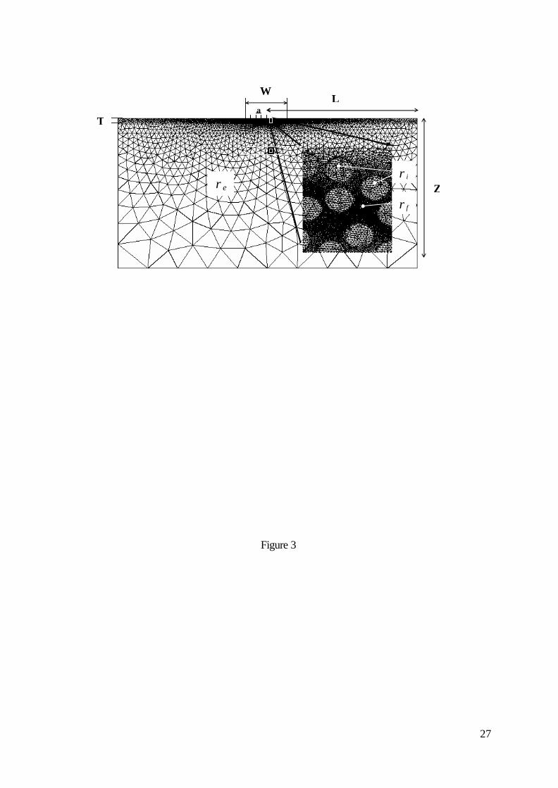
The model structure (figure 3) is composed of a heterogeneous rectangular body (dimensions W and

T, resistivity ρf) containing circular resistive inclusions having all the same properties (radius R,

resistivity ρi) and bordered by an external homogeneous zone (resistivity ρe). Various numerical tests

were conducted in order to ensure the validity of the F.E.A. model, using a mesh composed of

three-node elements.

The inclusions were non-jointed and randomly spread. As the current paths are mainly contained in

the conductive matrix, the presence of at least two layers of finite element was required between two

neighbouring inclusions, in order to not limit numerically the conduction of these areas. A minimal

distance of 0.2R was needed between two inclusions to ensure a sufficient spatial discretization,

limiting the possible percentage of inclusions to 40%. Moreover a minimum of two three-node

elements between two neighbouring electrodes was required. Such a dense spatial meshing limited

the possible size (W x T) of the heterogeneous rectangular body, the resistivity ρo of which were

studied.

The external zone was defined in order to move the boundaries of the mesh (Dirichlet condition,

V=0) away from the central investigated area. It was shown that the distance L between the centre

of the mesh and its boundaries (figure 3) must be 15 times greater than the electrode spacing a, to

contain the error on resistivity values below 0.5%. So the simulated sequence of measurements (with

spacing varying from amin to amax) had to respect the condition L/amax ≥15.

The resistivity of the external zone ρe was fixed thanks to Bussian’s relashionship, using a

cementation factor m=2 (2D, circular inclusions). The influence of this area on the current paths was

analysed and a correction procedure was set up to clear the results from this disturbance.

9

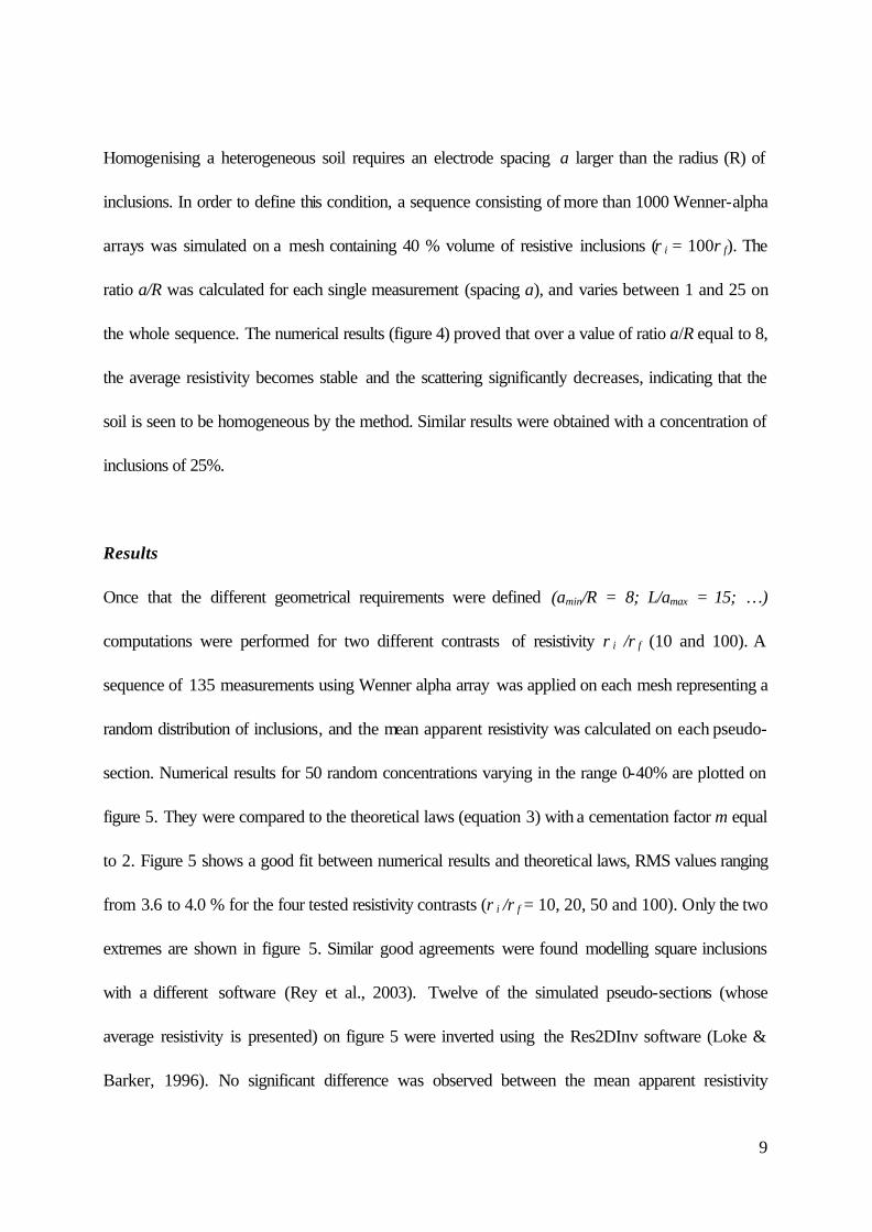
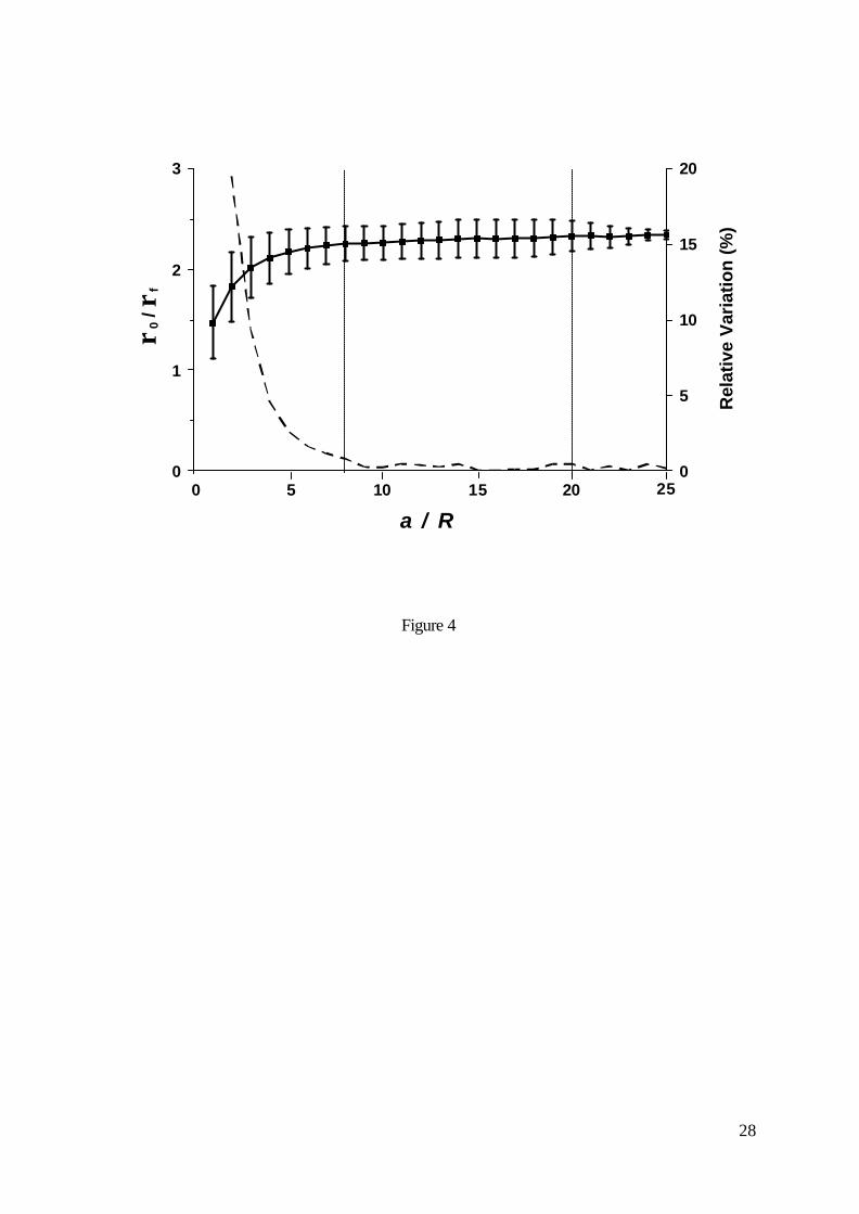
Homogenising a heterogeneous soil requires an electrode spacing a larger than the radius (R) of

inclusions. In order to define this condition, a sequence consisting of more than 1000 Wenner-alpha

arrays was simulated on a mesh containing 40 % volume of resistive inclusions (ρi = 100ρf). The

ratio a/R was calculated for each single measurement (spacing a), and varies between 1 and 25 on

the whole sequence. The numerical results (figure 4) proved that over a value of ratio a/R equal to 8,

the average resistivity becomes stable and the scattering significantly decreases, indicating that the

soil is seen to be homogeneous by the method. Similar results were obtained with a concentration of

inclusions of 25%.

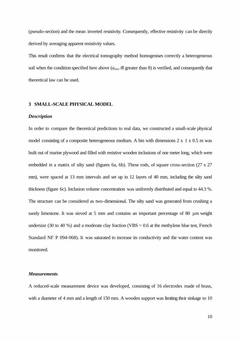
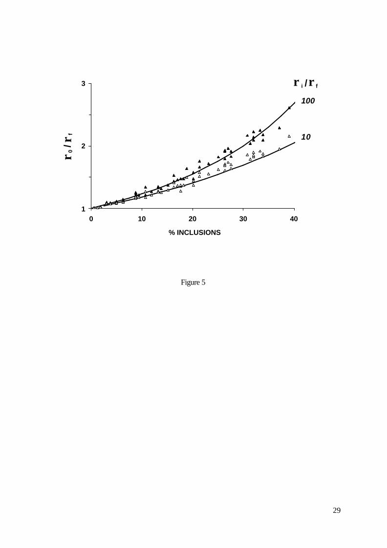
Results

Once that the different geometrical requirements were defined (amin/R = 8; L/amax = 15; …)

computations were performed for two different contrasts of resistivity ρi /ρf (10 and 100). A

sequence of 135 measurements using Wenner alpha array was applied on each mesh representing a

random distribution of inclusions, and the mean apparent resistivity was calculated on each pseudo-

section. Numerical results for 50 random concentrations varying in the range 0-40% are plotted on

figure 5. They were compared to the theoretical laws (equation 3) with a cementation factor m equal

to 2. Figure 5 shows a good fit between numerical results and theoretical laws, RMS values ranging

from 3.6 to 4.0 % for the four tested resistivity contrasts (ρi /ρf = 10, 20, 50 and 100). Only the two

extremes are shown in figure 5. Similar good agreements were found modelling square inclusions

with a different software (Rey et al., 2003). Twelve of the simulated pseudo-sections (whose

average resistivity is presented) on figure 5 were inverted using the Res2DInv software (Loke &

Barker, 1996). No significant difference was observed between the mean apparent resistivity

10

(pseudo-section) and the mean inverted resistivity. Consequently, effective resistivity can be directly

derived by averaging apparent resistivity values.

This result confirms that the electrical tomography method homogenises correctly a heterogeneous

soil when the condition specified here above (amin /R greater than 8) is verified, and consequently that

theoretical law can be used.

3 SMALL-SCALE PHYSICAL MODEL

Description

In order to compare the theoretical predictions to real data, we constructed a small-scale physical

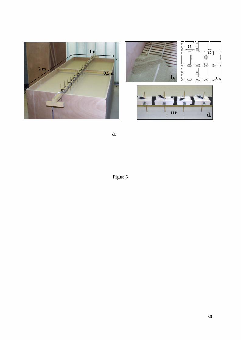
model consisting of a composite heterogeneous medium. A bin with dimensions 2 x 1 x 0.5 m was

built out of marine plywood and filled with resistive wooden inclusions of one meter long, which were

embedded in a matrix of silty sand (figures 6a, 6b). These rods, of square cross-section (27 x 27

mm), were spaced at 13 mm intervals and set up in 12 layers of 40 mm, including the silty sand

thickness (figure 6c). Inclusion volume concentration was uniformly distributed and equal to 44.3 %.

The structure can be considered as two-dimensional. The silty sand was generated from crushing a

sandy limestone. It was sieved at 5 mm and contains an important percentage of 80 µm weight

undersize (30 to 40 %) and a moderate clay fraction (VBS = 0.6 at the methylene blue test, French

Standard NF P 094-068). It was saturated to increase its conductivity and the water content was

monitored.

Measurements

A reduced-scale measurement device was developed, consisting of 16 electrodes made of brass,

with a diameter of 4 mm and a length of 150 mm. A wooden support was limiting their sinkage to 10

11

mm. They were spaced every 110 mm (figure 6d), so the homogenization condition (amin/R ≥ 8) was

respected since the inclusions are assumed to be cylindrical rods with a radius of 13.5 mm. A

sequence of measurements was carried out on the full bin with an Iris Syscal R1+ as resistivity

recorder.

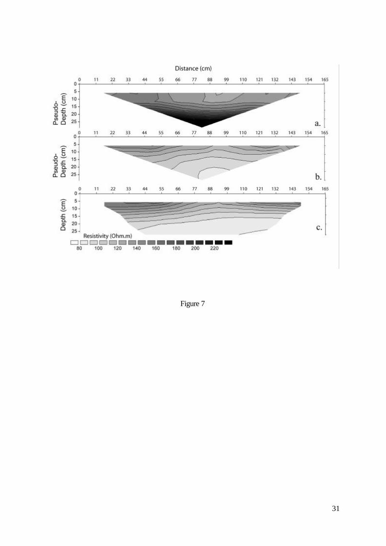
The raw pseudo-section (figure 7a) shows an important vertical gradient of resistivity due to the

effect of the marine plywood envelop box whose resistivity is about 1000 times greater than its

content. The 3D-effect of the resistive box was simulated with the finite-element code and the

corresponding correction was applied on the raw data. The corrected pseudo-section (figure 7b)

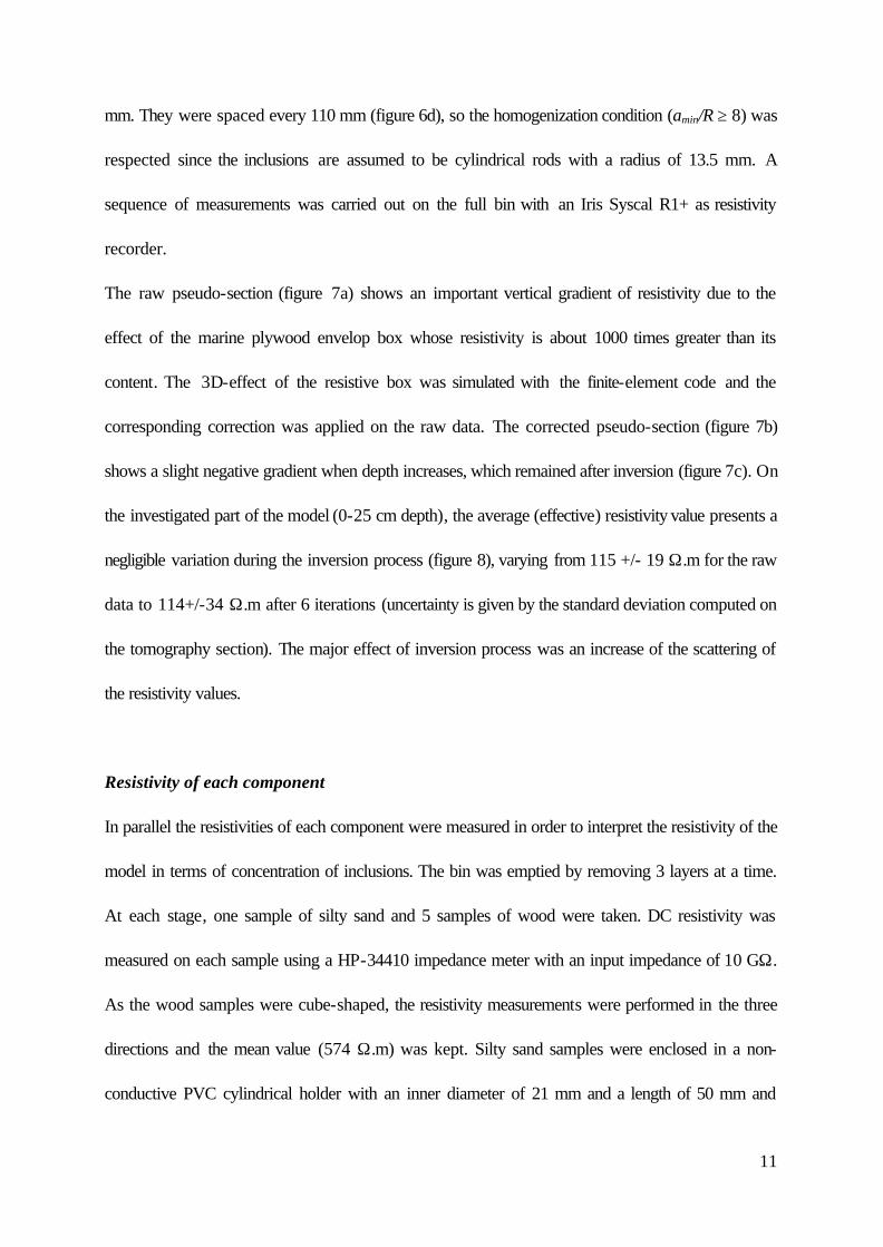
shows a slight negative gradient when depth increases, which remained after inversion (figure 7c). On

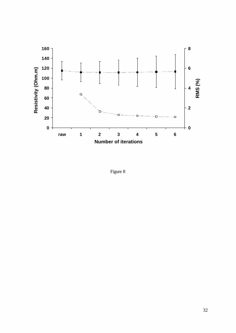
the investigated part of the model (0-25 cm depth), the average (effective) resistivity value presents a

negligible variation during the inversion process (figure 8), varying from 115 +/- 19 Ω.m for the raw

data to 114+/-34 Ω.m after 6 iterations (uncertainty is given by the standard deviation computed on

the tomography section). The major effect of inversion process was an increase of the scattering of

the resistivity values.

Resistivity of each component

In parallel the resistivities of each component were measured in order to interpret the resistivity of the

model in terms of concentration of inclusions. The bin was emptied by removing 3 layers at a time.

At each stage, one sample of silty sand and 5 samples of wood were taken. DC resistivity was

measured on each sample using a HP-34410 impedance meter with an input impedance of 10 GΩ.

As the wood samples were cube-shaped, the resistivity measurements were performed in the three

directions and the mean value (574 Ω.m) was kept. Silty sand samples were enclosed in a non-

conductive PVC cylindrical holder with an inner diameter of 21 mm and a length of 50 mm and

12

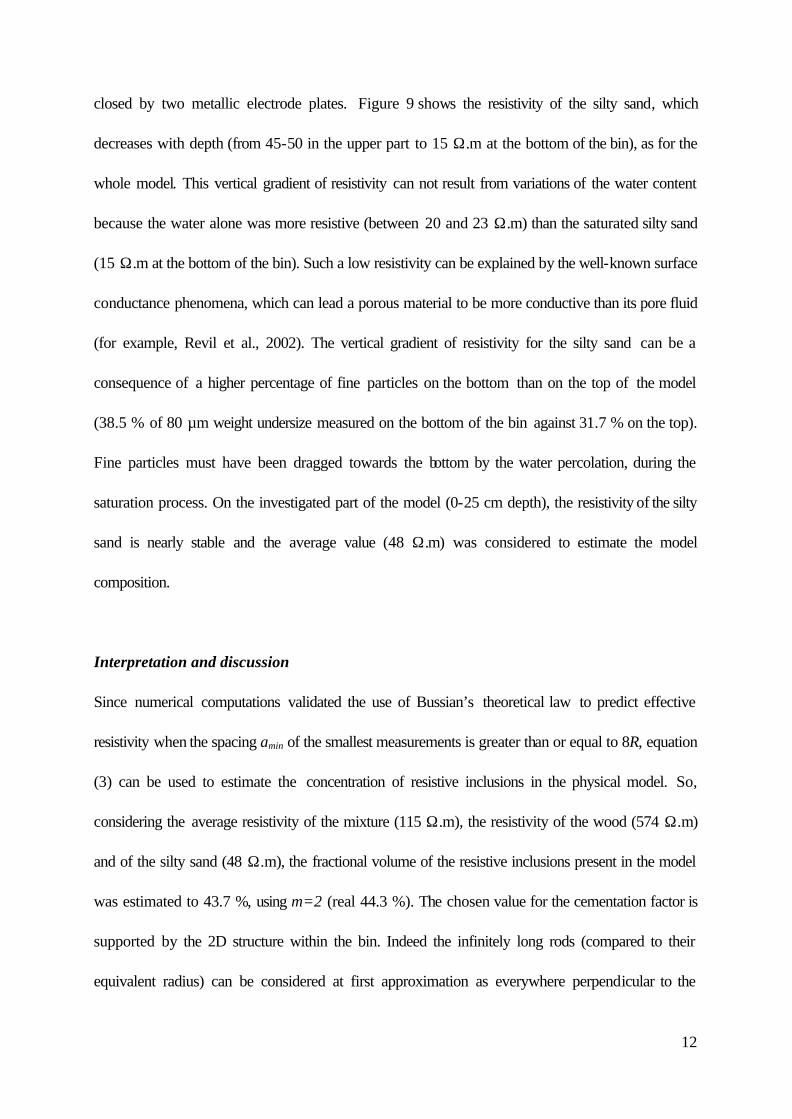
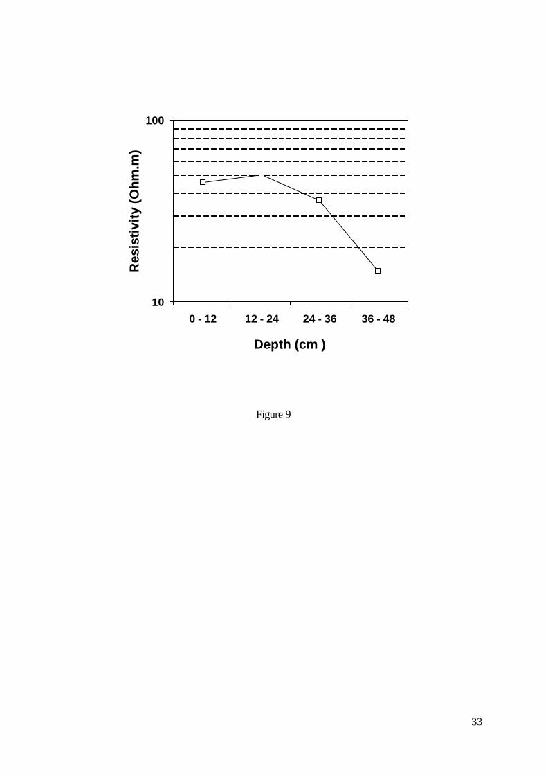
closed by two metallic electrode plates. Figure 9 shows the resistivity of the silty sand, which

decreases with depth (from 45-50 in the upper part to 15 Ω.m at the bottom of the bin), as for the

whole model. This vertical gradient of resistivity can not result from variations of the water content

because the water alone was more resistive (between 20 and 23 Ω.m) than the saturated silty sand

(15 Ω.m at the bottom of the bin). Such a low resistivity can be explained by the well-known surface

conductance phenomena, which can lead a porous material to be more conductive than its pore fluid

(for example, Revil et al., 2002). The vertical gradient of resistivity for the silty sand can be a

consequence of a higher percentage of fine particles on the bottom than on the top of the model

(38.5 % of 80 µm weight undersize measured on the bottom of the bin against 31.7 % on the top).

Fine particles must have been dragged towards the bottom by the water percolation, during the

saturation process. On the investigated part of the model (0-25 cm depth), the resistivity of the silty

sand is nearly stable and the average value (48 Ω.m) was considered to estimate the model

composition.

Interpretation and discussion

Since numerical computations validated the use of Bussian’s theoretical law to predict effective

resistivity when the spacing amin of the smallest measurements is greater than or equal to 8R, equation

(3) can be used to estimate the concentration of resistive inclusions in the physical model. So,

considering the average resistivity of the mixture (115 Ω.m), the resistivity of the wood (574 Ω.m)

and of the silty sand (48 Ω.m), the fractional volume of the resistive inclusions present in the model

was estimated to 43.7 %, using m=2 (real 44.3 %). The chosen value for the cementation factor is

supported by the 2D structure within the bin. Indeed the infinitely long rods (compared to their

equivalent radius) can be considered at first approximation as everywhere perpendicular to the

13

electrical field. The exact concentration (44.3 %) is reached for a m value of 1.95. This slight

decrease can be explained by the 3D current propagation (m=1.5 in 3D). Nevertheless these results

prove, as for numerical modelling, that Bussian’s relationships can be used to link the effective

resistivity of a mixture to its characteristics with a good precision.

4 FIELD MEASUREMENTS

Experimental site

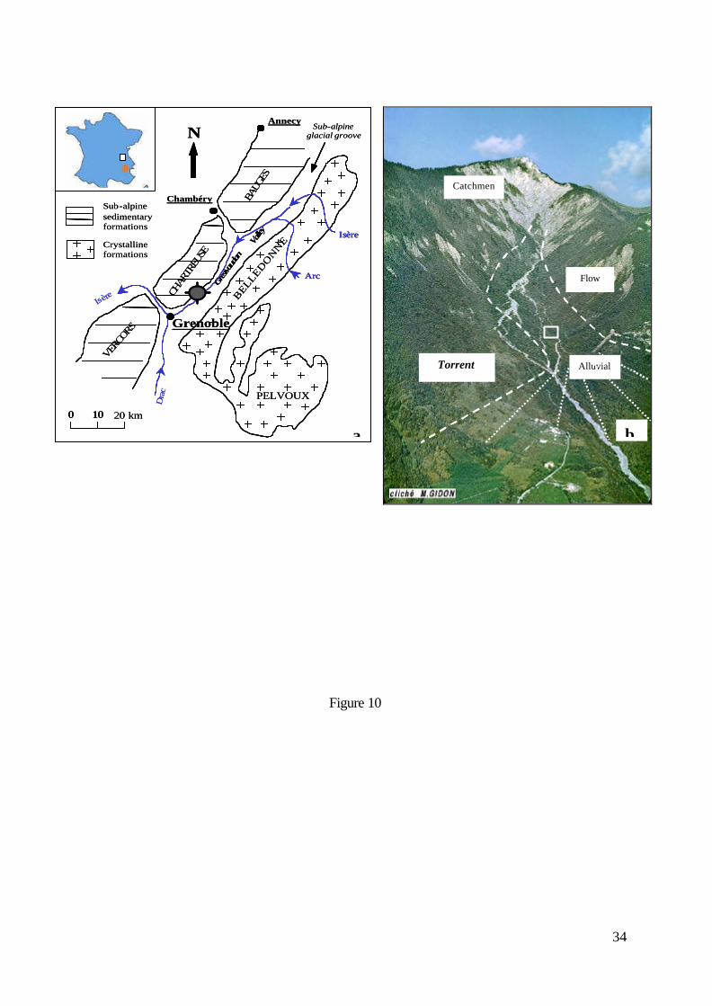
To apply our methodology under real conditions, an experimental site was investigated, localised 15

km North of Grenoble, in the Gresivaudan Valley (France). This important NE-SW glacial groove

separates the crystalline mountain chain of Belledonne to the East and the sedimentary mountain

chain of Chartreuse located to the West. On the eastern boundary of the latter range of mountain, the

sedimentary formations are eroded perpendicularly to the Gresivaudan Valley (toward NW) by the

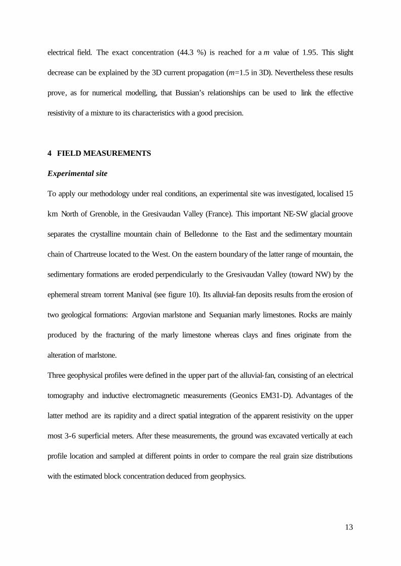
ephemeral stream torrent Manival (see figure 10). Its alluvial-fan deposits results from the erosion of

two geological formations: Argovian marlstone and Sequanian marly limestones. Rocks are mainly

produced by the fracturing of the marly limestone whereas clays and fines originate from the

alteration of marlstone.

Three geophysical profiles were defined in the upper part of the alluvial-fan, consisting of an electrical

tomography and inductive electromagnetic measurements (Geonics EM31-D). Advantages of the

latter method are its rapidity and a direct spatial integration of the apparent resistivity on the upper

most 3-6 superficial meters. After these measurements, the ground was excavated vertically at each

profile location and sampled at different points in order to compare the real grain size distributions

with the estimated block concentration deduced from geophysics.

14

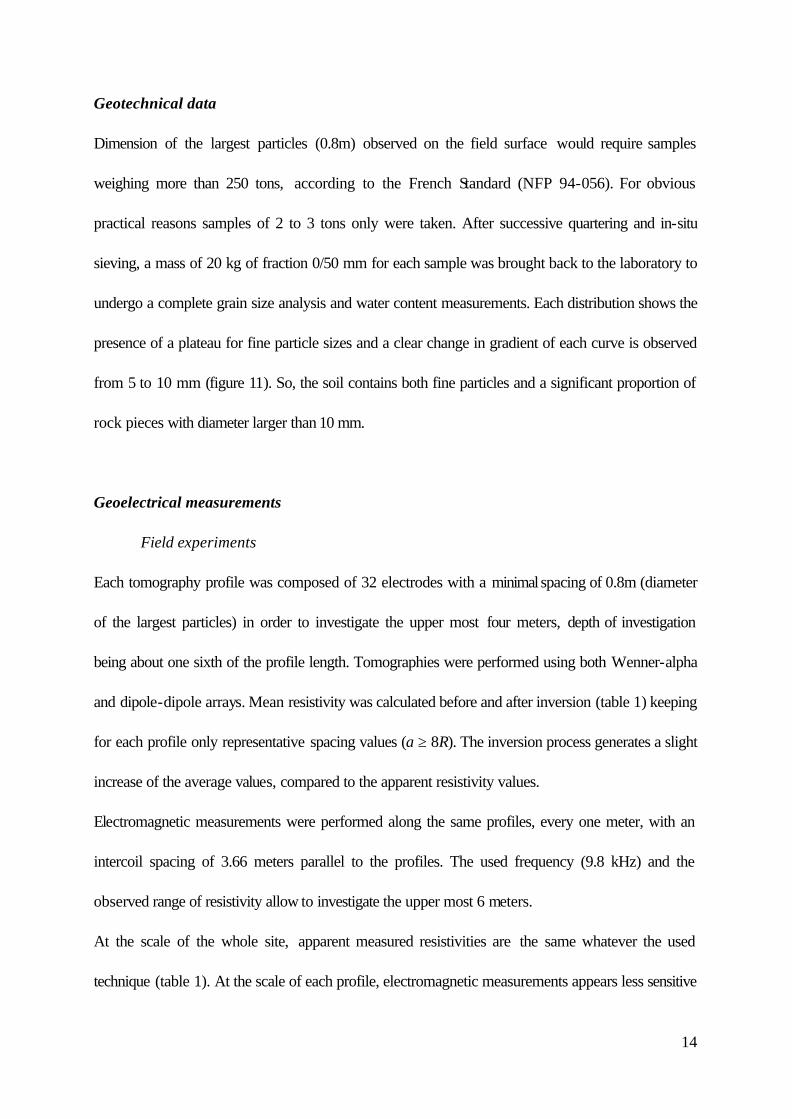
Geotechnical data

Dimension of the largest particles (0.8m) observed on the field surface would require samples

weighing more than 250 tons, according to the French Standard (NFP 94-056). For obvious

practical reasons samples of 2 to 3 tons only were taken. After successive quartering and in-situ

sieving, a mass of 20 kg of fraction 0/50 mm for each sample was brought back to the laboratory to

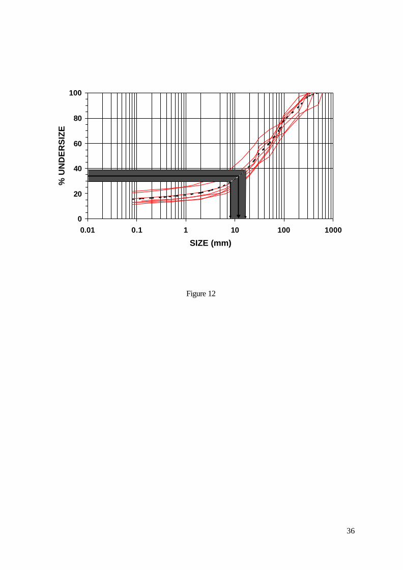
undergo a complete grain size analysis and water content measurements. Each distribution shows the

presence of a plateau for fine particle sizes and a clear change in gradient of each curve is observed

from 5 to 10 mm (figure 11). So, the soil contains both fine particles and a significant proportion of

rock pieces with diameter larger than 10 mm.

Geoelectrical measurements

Field experiments

Each tomography profile was composed of 32 electrodes with a minimal spacing of 0.8m (diameter

of the largest particles) in order to investigate the upper most four meters, depth of investigation

being about one sixth of the profile length. Tomographies were performed using both Wenner-alpha

and dipole-dipole arrays. Mean resistivity was calculated before and after inversion (table 1) keeping

for each profile only representative spacing values (a ≥ 8R). The inversion process generates a slight

increase of the average values, compared to the apparent resistivity values.

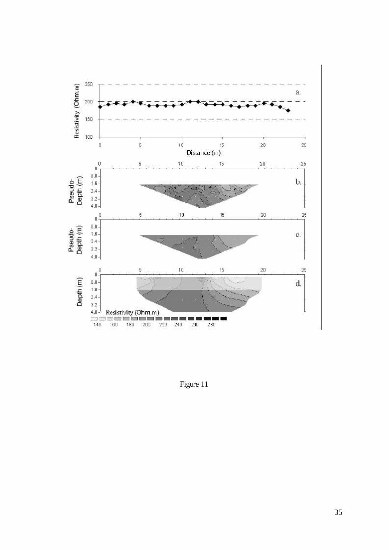
Electromagnetic measurements were performed along the same profiles, every one meter, with an

intercoil spacing of 3.66 meters parallel to the profiles. The used frequency (9.8 kHz) and the

observed range of resistivity allow to investigate the upper most 6 meters.

At the scale of the whole site, apparent measured resistivities are the same whatever the used

technique (table 1). At the scale of each profile, electromagnetic measurements appears less sensitive

15

to the lateral slight variations of resistivity, as shown on figure 12 representing in parallel EM and

tomographic data for the P2 profile. It is probably due to its deeper integration, as well as the fact

that electrical tomography seems more open to lateral zoning.

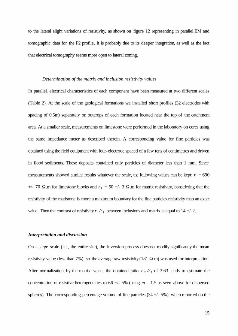
Determination of the matrix and inclusion resistivity values

In parallel, electrical characteristics of each component have been measured at two different scales

(Table 2). At the scale of the geological formations we installed short profiles (32 electrodes with

spacing of 0.5m) separately on outcrops of each formation located near the top of the catchment

area. At a smaller scale, measurements on limestone were performed in the laboratory on cores using

the same impedance meter as described therein. A corresponding value for fine particles was

obtained using the field equipment with four-electrode spaced of a few tens of centimetres and driven

in flood sediments. These deposits contained only particles of diameter less than 1 mm. Since

measurements showed similar results whatever the scale, the following values can be kept: ρi = 690

+/- 70 Ω.m for limestone blocks and ρf = 50 +/- 3 Ω.m for matrix resistivity, considering that the

resistivity of the marlstone is more a maximum boundary for the fine particles resistivity than an exact

value. Then the contrast of resistivity ρi /ρf between inclusions and matrix is equal to 14 +/-2.

Interpretation and discussion

On a large scale (i.e., the entire site), the inversion process does not modify significantly the mean

resistivity value (less than 7%), so the average raw resistivity (181 Ω.m) was used for interpretation.

After normalization by the matrix value, the obtained ratio ρ0 /ρf of 3.63 leads to estimate the

concentration of resistive heterogeneities to 66 +/- 5% (using m = 1.5 as seen above for dispersed

spheres). The corresponding percentage volume of fine particles (34 +/- 5%), when reported on the

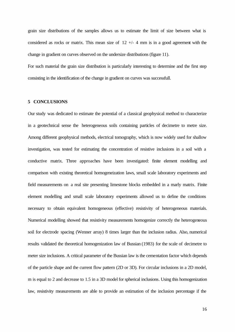
16

grain size distributions of the samples allows us to estimate the limit of size between what is

considered as rocks or matrix. This mean size of 12 +/- 4 mm is in a good agreement with the

change in gradient on curves observed on the undersize distributions (figure 11).

For such material the grain size distribution is particularly interesting to determine and the first step

consisting in the identification of the change in gradient on curves was successfull.

5 CONCLUSIONS

Our study was dedicated to estimate the potential of a classical geophysical method to characterize

in a geotechnical sense the heterogeneous soils containing particles of decimetre to metre size.

Among different geophysical methods, electrical tomography, which is now widely used for shallow

investigation, was tested for estimating the concentration of resistive inclusions in a soil with a

conductive matrix. Three approaches have been investigated: finite element modelling and

comparison with existing theoretical homogeneization laws, small scale laboratory experiments and

field measurements on a real site presenting limestone blocks embedded in a marly matrix. Finite

element modelling and small scale laboratory experiments allowed us to define the conditions

necessary to obtain equivalent homogeneous (effective) resistivity of heterogeneous materials.

Numerical modelling showed that resistivity measurements homogenize correctly the heterogeneous

soil for electrode spacing (Wenner array) 8 times larger than the inclusion radius. Also, numerical

results validated the theoretical homogenization law of Bussian (1983) for the scale of decimetre to

meter size inclusions. A critical parameter of the Bussian law is the cementation factor which depends

of the particle shape and the current flow pattern (2D or 3D). For circular inclusions in a 2D model,

m is equal to 2 and decrease to 1.5 in a 3D model for spherical inclusions. Using this homogenization

law, resistivity measurements are able to provide an estimation of the inclusion percentage if the

17

resistivity of the two phases is known. This method was satisfyingly confronted to a laboratory

experiment, for which the inclusion concentration was known. Finally, mean resistivities were

deduced from electrical tomographies and inductive EM measurements on a real site, where the grain

size distribution was independently characterized. Our measurements and interpretation showed that

the obtained limestone particle concentrations were consistent with the grain size data. Compared to

surface wave acquisition and processing, which also provide an estimation of the particle

concentration in the ground (Chammas et al. 2003), the main advantages of resistivity measurements

are their rapidity and the ability of obtaining a 2D image allowing lateral variations of particle

concentrations to be detected on a site.

ACKNOWLEDGEMENTS

The authors thank André Revil (CEREGE Aix-en-Provence, France) for allowing us to use his

equipment and for interesting and helpful discussions. We are grateful to Philippe Côte and Rabi

Chammas (LCPC Nantes, France) for their cooperation and informed advices about the finite

element code CESAR. LIRIGM is a member of the French network RNVO. This research was

supported by the “Pôle Grenoblois des Risques Naturels”.

REFERENCES

18

Abraham O., Chammas R., Côte Ph., Pedersen H.A., Semblat J.F., 2004. Mechanical

Characterisation of heterogeneous soils with surface waves : experimental validation on reduced-

scale physical models. Near Surface Geophysics, Vol. 2, n°4, 247- 258.

Archie G. E., 1942. The electrical resistivity log as an aid in determining some reservoir

characteristics. Petr. Tech. 1, 55-62.

Bourdeau Y., 1997. Le comportement des alluvions du Rhône dans une grande boîte de cisaillement

direct. Revue Française de Géotechnique 79, 45-57.

Bussian A.E., 1983. Electrical conductance in a porous medium. Geophysics, v.48, pp 1258-1268.

Chammas R., Abraham O., Côte Ph., Pedersen H.A., Semblat J.F., 2003. Characterization of

heterogeneous soils using surface waves : homogenization and numerical modelling. International

Journal of Geomechanics 3, 55-63.

Christensen R.M., Lo K.H., 1979. Solution for effective shear properties in three phase sphere and

cylinder models. J. Mech. Phys. Solids 27, 315-330.

Fagnoul A. et Bonnechere F., 1969. Shear strengh of porphyry materials. Proceedings of the 7th

International Conference on Soil Mechanics and Foundation Engineering. Special session

Mexico, 23-28 august 1969, 13, E1, 61-65.

19

French Standard NF P 94-056. Sols : Reconnaissance et essais. Analyse granulométrique. Méthode

par tamisage à sec après lavage. Ed. AFNOR, T1, 15p., 1996.

French Standard NFP 94-068. Sols : Reconnaissance et essais. Mesure de la quantité d’adsorption

de bleu de méthylène d’un sol ou d’un matériau rocheux. Détermination de la valeur au bleu de

méthylène d’un sol ou d’un matériau rocheux par l’essai à la tache. Ed. AFNOR, T1, 7p., 1998.

Holtz W.G., 1961. Triaxial shear characteristics of clayey gravel soils. Proceedings of the 5th

International Conference on Soil Mechanics and Foundation Engineering, Paris, 1961, 143-

149

Humbert P., 1989. CESAR-LCPC : Un code général de calcul par éléments finis. Bull. liaison des

Laboratoires des Ponts et Chaussées 160, 112-115

Jackson P. D., Taylor Smith D., Stanford P. N., 1978. Resitivity-porosity-particle shape

relationships for marine sands. Geophysics 43, 1250-1268.

Jongmans D. , Demanet D., 1993. The importance of surface waves in vibration study and the use of

Rayleigh waves for estimating the dynamics characteristics of soils. Engineering geology 34, 105-

113.

Loke M.H. & Barker R.D., 1996. Rapid least-squares inversion of apparent resistivity

pseudosections by a quasi-Newton method, Geophysical Prospecting 44, 131-152.

20

Mayne P. W., Rix G. J., 1995. Correlations between shear wave velocity and cone tip resistance in

natural clays . Soil and Foundations 35, n°2, 107-110

Mendelson K. S., Cohen M.H., 1982. The effect of grain anisotropy on the electrical properties of

sedimentary rocks to the dielectric constant of fused glass beads. Geophysics 47, 257-263.

Mestat P., 1997. Maillages d'éléments finis pour les ouvrages de géotechnique. Conseils et

recommandations. Bull.liaison des Laboratoires des Ponts et Chaussées 212, 39-64

Revil A., Hermitte D., Spangenberg E., Cochemé J.J., 2002. Electrical properties of zeolitized

volcanoclastic materials. J. Geophys. Res. 107 (B8), doi:10.1029/2001JB000599

Rey E., Garambois S., Jongmans D., Gotteland P., 2003. Characterisation of coarse materials using

geophysical methods. Proceedings of the 9th Meeting of Environmental and Engineering Geophysics,

Prague, O-061.

Reynolds J., 1997. An introduction to applied and environmental geophysics. Ed. Wiley, John &

Sons, Inc. 749 p.

Sen P.N., Scala C., Cohen M.H., 1981. A self-similar model for sedimentary rocks with application

to the dielectric constant of fused glass beads. Geophysics 46, 781-795.

21

Stokoe K.H., Nazarian S., Rix G.J., Sanchez-Salinero. I., Sheu J-C. and Mok Y.J., 1988. In situ

seismic testing of hard-to-sample soils by surface wave method. Earthquake Engineering and Soil

Dynamics II – Recent Advances in Ground Motion evaluation, Geotechnical special publication,

20, J.L. Von Thun, Ed. ASCE, New York, 64-278

22

FIGURE CAPTIONS

Figure 1: (a) Photography of an heterogeneous soil made of limestone rocks and particles embedded

in marly clay (Torrent Manival, France) - (b) Schematic view of a diphasic medium with resistive

inclusions in a conductive matrix.

Figure 2: A: Normalised effective resistivity (?0/?f) as a function of concentration of inclusions for a

cementation factor m=2 and a resistivity contrast ?f /?i =10 (after Bussian, 1983). B: The same as A

for a resistivity contrast of 100. C: Normalised bulk modulus K0/Kf for a shear wave velocity

contrast (Vsi/ Vsf) of 10 (Christensen and Lo, 1979).

Figure 3: Finite element model meshing used in the numerical modelling. L and Z denote respectively

the half length and the depth of the entire model. The heterogeneous rectangular body (large white

square contour, dimensions WxT ) is located on the top at the centre of the meshing. The zoom

shows that the host conductive medium (resistivity: ?f) is more densely meshed than the core of

inclusions (?i). ?e is the resistivity of the external homogenous zone.

Figure 4: Normalized effective resistivity (numerical results) as a function of ratio a/R for a

concentration of heterogeneities of 40 %. The dashed line represents the relative variation of ?0/?f ,

error band are statistical (standard deviation). Vertical lines delimit the range of a/R for which the soil

is seen to be homogeneous by the method (for a/R > 20, the influence of the external homogeneous

zone ρe becomes predominant).

23

Figure 5: Variation of the normalised effective resistivity as a function of the percentage of inclusions

for two resistivity contrasts (10 and 100). Numerical results (apparent normalised resistivity) are

computed for 50 random distributions of inclusions (with concentrations varying from 0 to 40 %).

Theoretical curves are calculated using Bussian’s law with a cementation factor m = 2.

Figure 6: Small-scale laboratory model. (a) Global view of the bin. (b) Layout of the 1 m long wood

rods embedded in silty sand. (c) Partial cross section showing the mixing of square rods and soil. (d)

Small-scale electrical measurement device. If not precised, dimensions are in millimetres.

Figure 7: Results of laboratory electrical tomography measurements. Investigation of layer 0-25 cm

depth : (a) pseudo-section data. (b) corrected pseudo-section data. (c) inverted resistivity model

(here RMS=1.6 % after 2 iterations).

Figure 8: Effective resistivity of the 25 most superficial centimetres of the model as a function of

number of iterations. Full line represents the mean resistivity with associate standard deviation, and

dashed line the RMS.

Figure 9: Laboratory resistivity measurements on silty sand as a function of the bin depth.

Figure 10: (a) Location of the real experimental site. (b) Global view of the erosion silted stream

Manival. The investigated area is located by the white square contour (photo M. Gidon, www.geol-

alp.com).

24

Figure 11: Grain size distributions (grey curves) of the seven samples taken in the Manival site. The

thick dashed curve is the mean. The mean inclusion percentage (66%) estimated by electrical

measurements, corresponding to 34 +/- 5% undersize, leads to a size limit of about 12 (mean : bold

arrow) +/- 4 mm (thin arrows) between matrix and inclusions.

Figure 12: Electrical measurements on profile P2. (a) Apparent resistivity data obtained from EM-31

measurements. (b) Measured pseudo-section from electrical tomography. Superficial non

representative values have been removed. (c) calculated pseudo-section (Res2Dinv). (d) True

resistivity model after inversion (RMS = 2.9%).

25

Figure 1

b.

a.

26

1

10

100

0 20 40 60 80 100

% INCLUSIONS

ρ O / ρ f

,

KO

/ K f

C

A

B

Figure 2

27

Figure 3

a T

W

ρe ρi

ρf

L

Z

28

0

1

2

3

1

a / R

Rel

ativ

e V

aria

tion

(%

)

0

5

10

15

20ρ 0

/ ρ f

5 15 20 25100

Figure 4

29

1

2

3

0 10 20 30 40

% INCLUSIONS

ρ 0 /

ρ fρ i / ρ f

100

10

Figure 5

30

Figure 6

a.

b.

d. 110

2 m

1 m

0,5 m

c.

31

Figure 7

32

0

20

40

60

80

100

120

140

160

raw 1 2 3 4 5 6

Number of iterations

Res

isti

vity

(O

hm

.m)

0

2

4

6

8

RM

S (%

)

Figure 8

33

10

100

0 - 12 12 - 24 24 - 36 36 - 48

Depth (cm )

Res

isti

vity

(Oh

m.m

)

Figure 9

34

Figure 10

0 10

Arc

Isère

Sub-alpine sedimentary formations

0 10 20 km

VERCO

RS

BAUG

ES

PELVOUX

Arc

IsèreB

E L L

E D O

N N

E

Isère CHAR

TREU

SE

Dra

c

Crystallineformations

NAnnecy

Grenoble

Chambéry

Gresi

vaud

an

Valley

Sub-alpineglacial groove

0 10

Arc

Isère

Sub-alpine sedimentary formations

0 10 20 km

VERCO

RS

BAUG

ES

PELVOUX

Arc

IsèreB

E L L

E D O

N N

E

Isère CHAR

TREU

SE

Dra

c

Crystallineformations

NAnnecy

Grenoble

Chambéry

Gresi

vaud

an

Valley

Sub-alpineglacial groove

a.

Catchmen

Flow

Alluvial

b.

Torrent

35

Figure 11

36

0

20

40

60

80

100

0.01 0.1 1 10 100 1000

SIZE (mm)

% U

ND

ER

SIZ

E

Figure 12

37

Resistivity Profile 1 Profile 2 Profile 3 Site

Apparent (DC) 192 +/- 12 201 +/- 13 151 +/- 14 181 +/- 26

True (inverted)

% RMS

204 +/- 7

2.5%

209 +/- 13

2.9%

169 +/- 9

3.4%

193 +/- 20

Apparent (EM 31) 186 +/- 7 191 +/- 5 172 +/- 14 183 +/- 12

Table 1

38

Scale ρi (Ω.m) ρf (Ω.m)

Centimetric Marly limestone : 665-880 Fines : 50+/-3

Decametric Sequanian marly limestone : 690 +/- 70 Argovian marlstone : 55+/- 3

Table 2