Characterisation of the benthos in the Big Russel, Guernsey

2011

Sheehan, E.V., Gall, S.C., & Attrill, M.A.

Peninsula Research Institute for Marine Renewable Energy (PRIMaRE), Marine

Institute, Plymouth University

2

Table of Contents

Table of figures ........................................................................................................ 3

Table of tables .......................................................................................................... 4

1. Introduction ........................................................................................................ 5

2. Methods .............................................................................................................. 7

2.1 Sampling methods ........................................................................................ 7

2.2 Site selection ................................................................................................. 8

2.3 Video analysis ............................................................................................... 9

2.4 Data analysis ............................................................................................... 11

3. Results & Discussion ...................................................................................... 12

3.1. Habitat types ............................................................................................... 13

3.2. Assemblage composition ............................................................................ 13

3.3. Assemblage composition and habitat type .................................................. 22

4. Conclusion ....................................................................................................... 26

Acknowledgements ................................................................................................ 27

References .............................................................................................................. 27

3

Table of figures

Figure 1.1

The Balliwick of Guernsey showing its location off the north coast of France. The Big Russel is marked as the channel running between the islands of Guernsey and Sark (Source: RET)

5

Figure 2.1 a) the vessel ‘Nicola May’ in port, b) & c) the flying array being deployed from the stern, d) the towed array submerging showing the umbilical (blue) and mid-water weights for stability

7

Figure 2.2 Flying array used for the towed video survey. a = high definition video camera, b = LED lights, c = lasers

8

Figure 2.3 Location of towed video transects (sites) used for analysis in the Big Russel and south of St Martins Point, Guernsey, September 2011. Sites are divided into Locations (A,B,C,D,E) and Areas (pairs or 3s of sites as shown by the dotted lines)

9

Figure 2.4 Diagrammatic representation of a frame grab with laser positions marked and numbered. Positions -1, 0 and 1 are acceptable for frame grab analysis

10

Figure 3.1 Percentage cover of each habitat type (rock, boulders, cobbles, pebbles, sand) from the frame data

13

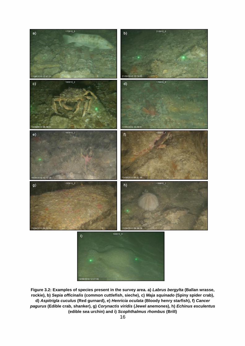
Figure 3.2 Examples of species present in the survey area. a) Labrus bergylta (Ballan wrasse, rockie), b) Sepia officinalis (Common cuttlefish, sieche), c) Maja squinado (Spiny spider crab), d) Aspitrigla cuculus (Red gurnard), e) Henricia oculata (Bloody henry starfish), f) Cancer pagurus (Edible crab, shanker), g) Corynactis viridis (Jewel anemones), h) Echinus esculentus (edible sea urchin) and i) Scophthalmus rhombus (Brill)

16

Figure 3.3 Examples of the most abundant taxa from video transects, a) Alcyonium digitatum (Dead man’s fingers), b) Pentapora fascialis (Ross coral), c) Grouped hydroids, d) Turf

17

Figure 3.4 Species richness and abundance of taxa taken from the frame analysis for sites summed over area and averaged for Location (A,B,C,D,E)

18

Figure 3.5 nonmetric Multi-Dimensional Scaling (nMDS) plot showing the similarities between main assemblage composition determined through frame analysis at sites in Locations A, B, C, D and E. Site 28 was removed from the analysis as no species were identified through the frame analysis

19

Figure 3.6 nonmetric Multi-Dimensional Scaling (nMDS) plot showing the similarities between composition of conspicuous sessile and mobile fauna determined through video transect analysis at sites in Locations A, B, C, D and E.

19

Figure 3.7 nonmetric Multi-Dimensional Scaling (nMDS) plot showing the similarities between species assemblages at different sites based on habitat type. Habitat type is the dominant type per tow calculated from the frame analysis (R (rock), B (boulders), C (cobbles), P (pebbles), G (gravel), and S (sand)), (see Table 2.2 for details)

23

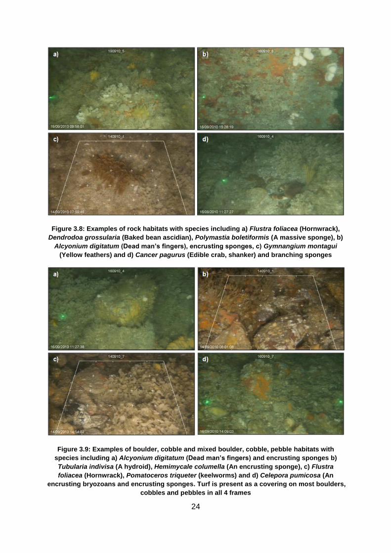
Figure 3.8 Examples of rock habitats with species including a) Flustra foliacea (Hornwrack), Dendrodoa grossularia (Baked bean ascidian), Polymastia boletiformis (A massive sponge), b) Alcyonium digitatum (Dead man’s fingers), encrusting sponges, c) Gymnangium montagui (Yellow feathers) and d) Cancer pagurus (Edible crab, shanker) and branching sponges

24

Figure 3.9 Examples of boulder, cobble and mixed boulder, cobble, pebble habitats with species including a) Alcyonium digitatum (Dead man’s fingers) and encrusting sponges b) Tubularia indivisa (A hydroid), Hemimycale columella (An encrusting sponge), c) Flustra foliacea (Hornwrack), Pomatoceros triqueter (keelworms) and d) Celepora pumicosa (An encrusting bryozoans and encrusting sponges. Turf is present as a covering on most boulders, cobbles and pebbles in all 4 frames

24

Figure 3.10 Examples of (a), gravel (b) gravel and sand and (c & d) sand habitats with species including d) grouped hydroids and red algae

25

4

Table of tables

Table 2.1 Descriptions of the sponges identified during the study and the name assigned to each. Where possible the species that each is thought to be is given. However, these are not exclusive and should be treated with caution, particularly for the encrusting species

12

Table 2.2 Habitat codes used for the video and frame analysis and their descriptions based on the Wentworth Scale. Sediment of < 2 mm is classified as sand as it was not possible to classify sediment smaller than this with accuracy

12

Table 3.1 Species list detailing the taxa present, listed in alphabetical order of species code, with species/taxa name, common name and local name also given, and details of the survey method(s) that recorded them

14

Table 3.2 Results of a) Permanova analysis for the relative distribution of the main assemblage species identified using frame data in response to the fixed factor Location (Lo) and random factors Area (Ar) and Site (Si) and their interactions, and b) pairwise testing for Location showing P values for the differences between Location pairings. Analyses were conducted using Bray Curtis similarities and data were dispersion weighted and square root transformed. P values in bold type are significant

17

Table 3.3 Results of a) Permanova analysis for the relative distribution of the conspicuous sessile and mobile species identified using video transect data in response to the fixed factor Location (Lo) and random factors Area (Ar) and Site (Si) and their interactions, and b) pairwise testing for Location showing P values for the differences between Location pairings. Analyses were conducted using Bray Curtis similarities and data were dispersion weighted and square root transformed. P values in bold type are significant

19

Table 3.4 Results of SIMPER analysis to determine the taxa whose abundance contributes most to the similarities seen between Locations for a) Frame and b) Video transect data. Average similarity (%) is given for sites within each Location along with average abundance (AvAbund) of the six species contributing most (Contrib%) to similarity of sites within each Location

21

Table 3.5 The ten species from frame analysis with the highest abundance (Ab.) where rock, boulders & cobbles and sand were the dominant habitat type. Data are percentage of frames containing each species for each habitat type. Gravel and pebbles were excluded as they did not dominate the habitat in any frame. Please refer to Table 3.1 for full species names

22

5

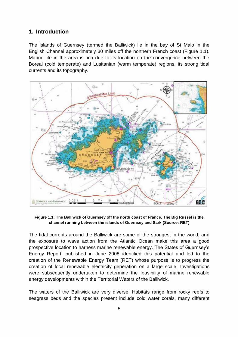
1. Introduction

The islands of Guernsey (termed the Balliwick) lie in the bay of St Malo in the

English Channel approximately 30 miles off the northern French coast (Figure 1.1).

Marine life in the area is rich due to its location on the convergence between the

Boreal (cold temperate) and Lusitanian (warm temperate) regions, its strong tidal

currents and its topography.

Figure 1.1: The Balliwick of Guernsey off the north coast of France. The Big Russel is the

channel running between the islands of Guernsey and Sark (Source: RET)

The tidal currents around the Balliwick are some of the strongest in the world, and

the exposure to wave action from the Atlantic Ocean make this area a good

prospective location to harness marine renewable energy. The States of Guernsey’s

Energy Report, published in June 2008 identified this potential and led to the

creation of the Renewable Energy Team (RET) whose purpose is to progress the

creation of local renewable electricity generation on a large scale. Investigations

were subsequently undertaken to determine the feasibility of marine renewable

energy developments within the Territorial Waters of the Balliwick.

The waters of the Balliwick are very diverse. Habitats range from rocky reefs to

seagrass beds and the species present include cold water corals, many different

6

sponges, and a range of fishes and crabs. It is essential that the impact of any

development occurring within the marine environment is minimal to protect these

habitats. For this reason, a Regional Environmental Assessment (REA) was

undertaken to determine the likely environmental impacts arising from the

development of wave and tidal energy production in the area. The document was

also designed to aid the development of marine environmental planning policy on the

islands and to inform subsequent Environmental Impact Assessments carried out by

independent energy developers. The benthic ecology section of the REA report

focussed on pre-existing information from online marine biological databases, the

Guernsey Biological Records Centre, Volunteer research programmes and UK

Government sources. Information regarding the habitats and associated species in

the Big Russel was lacking and so, to assess the potential future impact of marine

renewable development in this area and to identify particularly sensitive and/or

important habitats and species, a benthic survey was undertaken.

RET commissioned the Peninsula Research Institute for Marine Renewable Energy

(PRIMaRE), Marine Institute, Plymouth University to quantify the tide swept benthic

communities present in the Big Russel using a survey method newly developed at

Wave Hub, a renewable energy site off the north coast of Cornwall. The method was

developed specifically to survey benthic communities at renewable energy sites. It is

therefore cost-effective, relatively non-destructive and suitable for use over a range

of habitat types and sea conditions (Sheehan et al 2010).

The purpose of this study was to survey the Big Russel and document the various

habitats and associated flora and fauna. These data could be used in future to create

habitat maps, as a baseline account of the habitats and species present for future

tidal development impact assessment.

7

2. Methods

Benthic surveys were conducted in the Big Russel from 13th – 22nd September, 2010,

from the fishing trawler the ‘Nicola May’ (Figure 2.1a) skippered by Mr Shane Petit.

The aim of the survey was to document the benthos to provide a baseline of species

composition in an area where tidal development may occur, and to identify suitable

control areas for future comparison.

The strength of the tides in Guernsey were such that the established methodologies

had to be adapted, and the successful completion of the survey demonstrates the

suitability of the methodology detailed below for tidal conditions of up to 2.4 knots.

Figure 2.1: a) the vessel ‘Nicola May’ in port, b) & c) the flying array being deployed from the

stern, d) the towed array emerging showing the umbilical (blue) and drop-weights for stability

2.1 Sampling methods

A High Definition video system was used to survey the seabed. This comprised of a

camera (Surveyor-HD-J12 colour zoom titanium camera, 6000 m depth rated, 720p)

positioned at a 45° angle to the seabed, LED lights (Bowtech Products limited, LED-

1600-13, 1600 Lumen underwater LED) mounted either side and below the camera,

8

and two laser pointers (Figure 2.2). The two laser pointers were mounted to the

frame either side of the camera at a fixed distance apart which allowed calibration of

the field of view during data analysis (Figure 2.2). An umbilical connected the

camera to the surface control unit (Figure 2.1d). The camera system was mounted

on an aluminium frame, which was a positively buoyant ‘flying array’ (Figure 2.2) and

was grounded by a short length of chain to provide stability and allow it to fly at a

fixed height above the seabed (Sheehan et al., 2010). A drop-weight was also

attached to the tow rope to provide extra stability and minimize the effect of the pitch

and roll of the boat on the flying array (Figure 2.1d).

Figure 2.2: Flying array used for the video survey. a = high definition video camera, b = LED

lights, c = lasers

To fly the camera over the seabed to film the benthic organisms, the flying array was

deployed over the stern of the boat and towed slowly (0.4 knots) for approximately

200 m (Figure 2.1a-d).

This method was selected as it is cost-effective, allowing large areas to be surveyed

rapidly (e.g. Stevens & Connolly, 2005). It is also has minimal impact on the seabed,

which is essential for studies where there is interest in documenting change over

time as it avoids confounding the results with impacts resulting from the survey

method. The use of high definition video provides data of a high quality, and also a

data archive for future use.

2.2 Site selection

Sites were selected across the Big Russel to include the areas, which had been

identified as potential locations for the development of tidal energy and to document

the remaining areas to ensure that those selected were most suitable (Figure 2.3).

Surveys were also conducted to the south of St Martins Point to provide a control

area that will be un-impacted by future development, allowing the degree of change

caused by energy devices in the impacted sites to be measured.

9

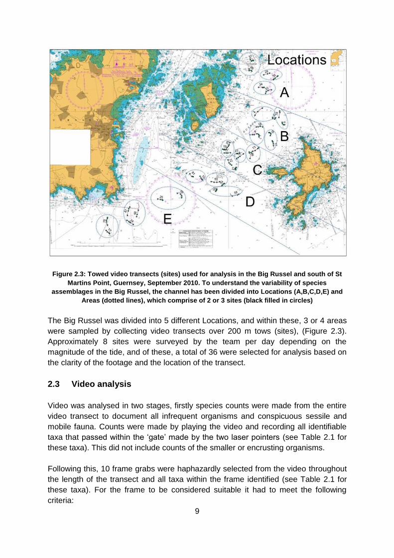
Figure 2.3: Towed video transects (sites) used for analysis in the Big Russel and south of St

Martins Point, Guernsey, September 2010. To understand the variability of species

assemblages in the Big Russel, the channel has been divided into Locations (A,B,C,D,E) and

Areas (dotted lines), which comprise of 2 or 3 sites (black filled in circles)

The Big Russel was divided into 5 different Locations, and within these, 3 or 4 areas

were sampled by collecting video transects over 200 m tows (sites), (Figure 2.3).

Approximately 8 sites were surveyed by the team per day depending on the

magnitude of the tide, and of these, a total of 36 were selected for analysis based on

the clarity of the footage and the location of the transect.

2.3 Video analysis

Video was analysed in two stages, firstly species counts were made from the entire

video transect to document all infrequent organisms and conspicuous sessile and

mobile fauna. Counts were made by playing the video and recording all identifiable

taxa that passed within the ‘gate’ made by the two laser pointers (see Table 2.1 for

these taxa). This did not include counts of the smaller or encrusting organisms.

Following this, 10 frame grabs were haphazardly selected from the video throughout

the length of the transect and all taxa within the frame identified (see Table 2.1 for

these taxa). For the frame to be considered suitable it had to meet the following

criteria:

10

i. Image must be well focussed

ii. Lasers must be within acceptable margins (positions -1, 0 or 1 (this was predetermined, see figure 2.4)

iii. Image must be clear of anything obstructing the view of the benthos (e.g.

large fish)

This method identified every species present within the frame and therefore provided

a means of quantifying the smaller and encrusting organisms that were not counted

using the video method.

Figure 2.4: Diagrammatic representation of a frame grab with laser positions marked and

numbered. Positions -1, 0 and 1 are acceptable for frame grab analysis

Taxa were identified to the lowest taxonomic level possible and recorded as density

per transect for the video counts and presence/absence for the frames. Where it was

not possible to identify taxa to species level some groupings were used as detailed

below:

i. The spider crabs Inachus spp. and Macropodia spp. were identified to genus

level as it was not possible to see the features necessary to identify these

organisms to species level.

ii. The hydroid species Halecium halecinum (Herring-bone hydroid),

Hydrallmania falcata and unidentified hydroids excepting Nemertesia ramosa,

11

Nemertesia antennina (Sea beard), Gymnangium montagui (Yellow feathers)

and Tubularia indivisa (Oaten pipes hydroid) were grouped due to the

difficulties associated with identifying them from the video (e.g. they are often

densely clumped together or coated in sediment).

iii. Goby species were grouped due to the difficulties in positively identifying them

from the video.

iv. Positive species identification of most sponges can only be made under

microscopic examination (Ackers et al., 2007). Branching, massive and

encrusting sponges that could not be identified with confidence were

numbered and identification was therefore made based on colour and

morphology with each number corresponding to what was thought to be a

different taxa. Table 2.1 details these. Other sponges (Cliona celata, (Boring

sponge) Dercitus bucklandi, Hemimycale columella, Pachymatisma johnstonia

(Elephant’s ear sponge), Polymastia boletiformis, and Suberites domuncula

(Sea-orange)) were identified to species level as they were considered to be

taxonomically distinct enough for a positive identification to be made.

v. Turf comprises hydroid and bryozoans turf which projects < 1 cm above the

seabed surface.

This report is accompanied by the dataset, so species codes are presented within

the report so that the dataset can be understood and used by RET in future.

2.4 Data analysis

To aid the understanding of the variability of species assemblages in the Big Russel,

the channel was spatially divided into different areas and the survey effort spread

throughout (Figure 2.3). To determine whether assemblages of organisms were

different between locations, the assemblage composition of the observed species

were compared using PERMANOVA (Anderson 2001) in PRIMER V6 (Clarke &

Warwick 2001). Multivariate results were visualised using nonmetric multi-

dimensional scaling (nMDS). In the nMDS displaying the species quantified using the

frame grabs, each point represented mean assemblage composition for one tow. In

the nMDS, to display the infrequent and conspicuous species, each point

represented the species observed over the entire 200 m tow.

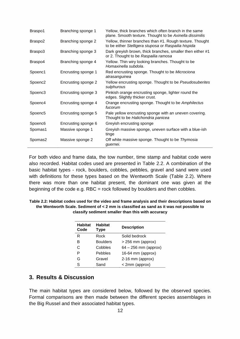
Table 2.1: Descriptions of the sponges identified during the study and the number and

suggested name assigned to each. Positive identification these species would require a

physical sample to be examined under a microscope.

Species code Taxa Description

12

Braspo1 Branching sponge 1 Yellow, thick branches which often branch in the same plane. Smooth texture. Thought to be Axinella dissimilis

Braspo2 Branching sponge 2 Yellow, thinner branches than #1. Rough texture. Thought to be either Stelligera stuposa or Raspailia hispida

Braspo3 Branching sponge 3 Dark greyish brown, thick branches, smaller then either #1 or 2. Thought to be Raspailia ramosa

Braspo4 Branching sponge 4 Yellow. Thin wiry looking branches. Thought to be Homaxinella subdola.

Spoenc1 Encrusting sponge 1 Red encrusting sponge. Thought to be Microciona atrasanguinea

Spoenc2 Encrusting sponge 2 Yellow encrusting sponge. Thought to be Pseudosuberites sulphurous

Spoenc3 Encrusting sponge 3 Pinkish orange encrusting sponge, lighter round the edges. Slightly thicker crust.

Spoenc4 Encrusting sponge 4 Orange encrusting sponge. Thought to be Amphilectus fucorum

Spoenc5 Encrusting sponge 5 Pale yellow encrusting sponge with an uneven covering. Thought to be Halichondria panicea

Spoenc6 Encrusting sponge 6 Greyish encrusting sponge

Spomas1 Massive sponge 1 Greyish massive sponge, uneven surface with a blue-ish tinge

Spomas2 Massive sponge 2 Off white massive sponge. Thought to be Thymosia guernei.

For both video and frame data, the tow number, time stamp and habitat code were

also recorded. Habitat codes used are presented in Table 2.2. A combination of the

basic habitat types - rock, boulders, cobbles, pebbles, gravel and sand were used

with definitions for these types based on the Wentworth Scale (Table 2.2). Where

there was more than one habitat present, the dominant one was given at the

beginning of the code e.g. RBC = rock followed by boulders and then cobbles.

Table 2.2: Habitat codes used for the video and frame analysis and their descriptions based on

the Wentworth Scale. Sediment of < 2 mm is classified as sand as it was not possible to

classify sediment smaller than this with accuracy

Habitat Code

Habitat Type

Description

R Rock Solid bedrock

B Boulders > 256 mm (approx)

C Cobbles 64 – 256 mm (approx)

P Pebbles 16-64 mm (approx)

G Gravel 2-16 mm (approx)

S Sand < 2mm (approx)

3. Results & Discussion

The main habitat types are considered below, followed by the observed species.

Formal comparisons are then made between the different species assemblages in

the Big Russel and their associated habitat types.

13

3.1. Habitat types

The survey area had a large diversity of habitat types ranging from sandy plains in

Location A in the far north east (site 28) to bedrock and rocky pinnacles in Locations

C & D, (Figure 3.1). Analysis of frame data showed that rock was present in the

majority of frames (36.34 %) (Figure 3.1), with 31.34 % composed entirely of

bedrock. Cobbles and boulders were the next most common habitats, occurring in

27.05 % and 18.43 % of frames respectively (Figure 3.1), and 13.68 % of frames as

combined habitat (BC).

36.34%

18.43%

27.05%

11.71%

6.47%

Rock

Boulders

Cobbles

Pebbles

Sand

Figure 3.1: Percentage cover of each habitat type (rock, boulders, cobbles, pebbles, sand)

from the frame data

3.2. Assemblage composition

A total of 74 taxa were identified during the survey, 39 from video transects and 59

from frame analysis. Table 3.1 gives a complete list of taxa identified in the Big

Russel, and Figure 3.2 shows images of some of these (Labrus bergylta (Ballan

wrasse, rockie), Sepia officinalis (Common cuttlefish, sieche), Maja squinado (Spiny

spider crab), Aspitrigla cuculus (Red gurnard), Henricia oculata (Bloody henry

starfish), Cancer pagurus (Edible crab, shanker), Corynactis viridis (Jewel

anemones), Echinus esculentus (edible sea urchin), and in the north of the Big

Russel where it is sandy, flatfishes such as Scophthalmus rhombus (Brill)).

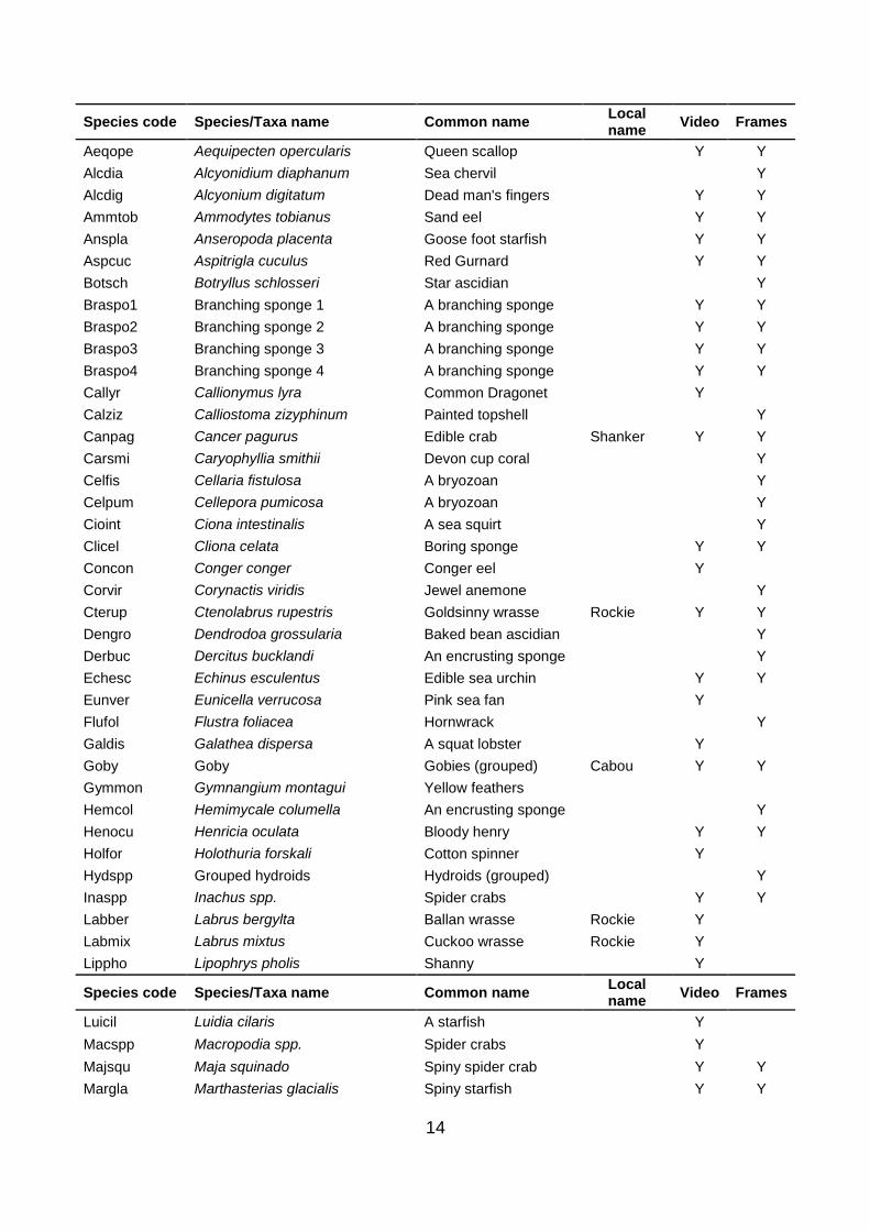
Table 3.1: Species list detailing the taxa present, listed in alphabetical order of species code,

with species/taxa name, common name and local name, and details of the survey method(s)

that recorded them

14

Species code Species/Taxa name Common name Local name

Video Frames

Aeqope Aequipecten opercularis Queen scallop Y Y

Alcdia Alcyonidium diaphanum Sea chervil Y

Alcdig Alcyonium digitatum Dead man's fingers Y Y

Ammtob Ammodytes tobianus Sand eel Y Y

Anspla Anseropoda placenta Goose foot starfish Y Y

Aspcuc Aspitrigla cuculus Red Gurnard Y Y

Botsch Botryllus schlosseri Star ascidian Y

Braspo1 Branching sponge 1 A branching sponge Y Y

Braspo2 Branching sponge 2 A branching sponge Y Y

Braspo3 Branching sponge 3 A branching sponge Y Y

Braspo4 Branching sponge 4 A branching sponge Y Y

Callyr Callionymus lyra Common Dragonet Y

Calziz Calliostoma zizyphinum Painted topshell Y

Canpag Cancer pagurus Edible crab Shanker Y Y

Carsmi Caryophyllia smithii Devon cup coral Y

Celfis Cellaria fistulosa A bryozoan Y

Celpum Cellepora pumicosa A bryozoan Y

Cioint Ciona intestinalis A sea squirt Y

Clicel Cliona celata Boring sponge Y Y

Concon Conger conger Conger eel Y

Corvir Corynactis viridis Jewel anemone Y

Cterup Ctenolabrus rupestris Goldsinny wrasse Rockie Y Y

Dengro Dendrodoa grossularia Baked bean ascidian Y

Derbuc Dercitus bucklandi An encrusting sponge Y

Echesc Echinus esculentus Edible sea urchin Y Y

Eunver Eunicella verrucosa Pink sea fan Y

Flufol Flustra foliacea Hornwrack Y

Galdis Galathea dispersa A squat lobster Y

Goby Goby Gobies (grouped) Cabou Y Y

Gymmon Gymnangium montagui Yellow feathers

Hemcol Hemimycale columella An encrusting sponge Y

Henocu Henricia oculata Bloody henry Y Y

Holfor Holothuria forskali Cotton spinner Y

Hydspp Grouped hydroids Hydroids (grouped) Y

Inaspp Inachus spp. Spider crabs Y Y

Labber Labrus bergylta Ballan wrasse Rockie Y

Labmix Labrus mixtus Cuckoo wrasse Rockie Y

Lippho Lipophrys pholis Shanny Y

Species code Species/Taxa name Common name Local name

Video Frames

Luicil Luidia cilaris A starfish Y

Macspp Macropodia spp. Spider crabs Y

Majsqu Maja squinado Spiny spider crab Y Y

Margla Marthasterias glacialis Spiny starfish Y Y

15

Necpub Necora puber Velvet swimming crab Lady crab Y Y

Nemant Nemertesia antennina Sea beard Y

Nemram Nemertesia ramosa A hydroid Y

Ophoph Ophiura ophiura A brittlestar Y

Pacjoh Pachymatisma johnstonia A sponge Y

Pargat Parablennius gattorugine Tompot Blenny Y Y

Pecmax Pecten maximus Great scallop Y Y

Penfas Pentapora foliacea Ross coral Y Y

Phogun Pholis gunnellus Butterfish Y

Polbol Polymastia boletiformis A sponge Y Y

Pomtri Pomatoceros triqueter Keelworm Y

Rajcla Raja clavata Thornback ray Y

Redalg Red algae Red algae (grouped) Y

Sabpav Sabella pavonina Peacock worm Y

Sagele Sagartia elegans A sea anemone Y

Sepoff Sepia officinalis Common cuttlefish Sieche Y Y

Server Serpula vermicularis A tubeworm Y

Spoenc1 Encrusting sponge 1 An encrusting sponge Y

Spoenc2 Encrusting sponge 2 An encrusting sponge Y

Spoenc3 Encrusting sponge 3 An encrusting sponge Y

Spoenc4 Encrusting sponge 4 An encrusting sponge Y

Spoenc5 Encrusting sponge 5 An encrusting sponge Y

Spoenc6 Encrusting sponge 6 An encrusting sponge Y

Spomas1 Massive sponge 1 A massive sponge Y

Spomas2 Massive sponge 2 A massive sponge Y

Subdom Suberites domuncula Sea orange Y

Trilus Trisopterus luscus Pouting Y

Trimin Trisopterus minutus Poor-cod Y

Tubind Tubularia indivisa A hydroid Y

Turf Turf Turf Y

Zeupun Zeugopterus punctatus Topknot Y Y

Frames that were composed entirely of bedrock were those with the greatest number

of species, with 44 of the 59 species recorded occurring here. Cobbles and pebbles

(CP) supported the second greatest abundance of species (32) followed by boulders

and cobbles (BC) (27). Although there were some mobile fauna such as flatfish in

the sandy habitat, no organisms appeared in the random frame grabs. The greatest

abundance of fauna in sedimentary habitats occurs below the surface ‘infauna’,

which the video does not sample. To quantify infauna would require dredges or a

grab to take physical samples.

16

Figure 3.2: Examples of species present in the survey area. a) Labrus bergylta (Ballan wrasse,

rockie), b) Sepia officinalis (common cuttlefish, sieche), c) Maja squinado (Spiny spider crab),

d) Aspitrigla cuculus (Red gurnard), e) Henricia oculata (Bloody henry starfish), f) Cancer

pagurus (Edible crab, shanker), g) Corynactis viridis (Jewel anemones), h) Echinus esculentus

(edible sea urchin) and i) Scophthalmus rhombus (Brill)

17

Alcyonium digitatum (dead man’s fingers) was the most abundant taxa identified

from the video transects (mean abundance of 158.86 ± 27.44 ind. tow-1), (Figure

3.3a) followed by Pentapora fascialis (ross coral), (mean abundance 86.91 ± 19.35

ind. tow-1), (Figure 3.3b). The most common taxa in the frame grabs was ‘grouped

hydroids’, which were present in 87.5 % of the frames (Figure 3.3c) followed by Turf

which was present in 75.5 % (Figure 3.3d).

a) b)

d) c)

Figure 3.3: Examples of the most abundant taxa from video transects, a) Alcyonium digitatum

(Dead man’s fingers), b) Pentapora fascialis (Ross coral), c) Grouped hydroids, d) Turf

Table 3.2: Results of a) Permanova analysis for the relative distribution of the main

assemblage species identified using frame data in response to the fixed factor Location (Lo)

and random factors Area (Ar) and Site (Si) and their interactions, and b) pairwise testing for

Location showing P values for the differences between Location pairings. Analyses were

conducted using Bray Curtis similarities and data were dispersion weighted and square root

transformed. P values in bold type are significant

a) b)

Source df Location pairings

MS Pseudo-F P(perm) P(perm)

Lo 4 2246.6 1.9995 0.0029 A & B 0.1719

Ar(Lo) 11 1125.4 1.2587 0.0825 A & C 0.1233

Si(Ar(Lo)) 16 894.08 No test A & D 0.4978

Total 31 A & E 0.4014

B & C 0.1127

B & D 0.0270

B & E 0.0107

C & D 0.0218

C & E 0.0047

D & E 0.0470

18

The assemblage composition of benthic fauna in the Big Russel was significantly

different between locations (for both video transect and frame analysis), (both P <

0.05, Tables 3.2a & 3.4a). In the middle of the Big Russel, Location C had the

greatest abundance of taxa, and Location D the greatest species richness (Figure

3.4). Location E, south of St Martin’s Point had a considerably lower abundance and

richness of taxa than in the locations in the main channel.

Figure 3.4: Species richness (no. of taxa) and abundance of individuals taken from the frame

analysis for sites summed over area and averaged for Location (A,B,C,D,E)

Pairwise testing for species assemblage composition (Table 3.2b) showed that

Location A was not significantly different to any other Location, but most other

Locations were significantly different to each other (Table 3.2b). It must be

considered however, that one of the sites in Location A (Site 28) was dominated by

sand and no species were identified during the frame analysis for the entire length of

the transect. When the similarities between sites were represented using an nMDS

plot (Figures 3.5 & 3.7) the differences between this site and the remaining sites

were such that it had to be removed in order to visualise the remaining sites. Most

species assemblage compositions were significantly different to each other (Table

3.2, significance indicated by P < 0.05), but these differences were not clear to see in

the nMDS, (Figure 3.5).

19

Figure 3.5: nonmetric Multi-Dimensional Scaling (nMDS) plot showing the similarities between

main assemblage composition determined through frame analysis at sites in Locations A, B,

C, D and E. Site 28 was removed as no species were identified through frame analysis

The assemblage composition of conspicuous sessile and mobile fauna between

Locations was also significantly different (P < 0.05, Table 3.4a), which is clear to see

in the nMDS (Figure 3.6).

Figure 3.6: nonmetric Multi-Dimensional Scaling (nMDS) plot showing the similarities between

composition of conspicuous sessile and mobile fauna determined through video transect

analysis at sites in Locations A, B, C, D and E.

20

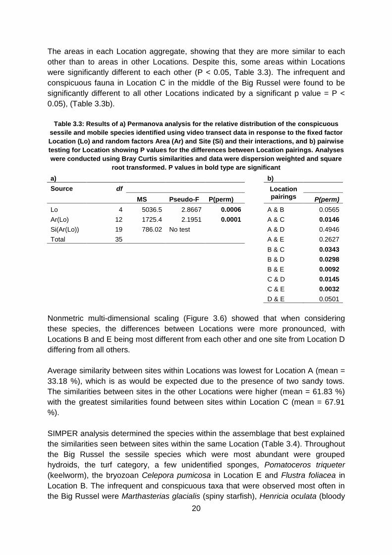
The areas in each Location aggregate, showing that they are more similar to each

other than to areas in other Locations. Despite this, some areas within Locations

were significantly different to each other (P < 0.05, Table 3.3). The infrequent and

conspicuous fauna in Location C in the middle of the Big Russel were found to be

significantly different to all other Locations indicated by a significant p value = P <

0.05), (Table 3.3b).

Table 3.3: Results of a) Permanova analysis for the relative distribution of the conspicuous

sessile and mobile species identified using video transect data in response to the fixed factor

Location (Lo) and random factors Area (Ar) and Site (Si) and their interactions, and b) pairwise

testing for Location showing P values for the differences between Location pairings. Analyses

were conducted using Bray Curtis similarities and data were dispersion weighted and square

root transformed. P values in bold type are significant

a) b)

Source df Location pairings

MS Pseudo-F P(perm) P(perm)

Lo 4 5036.5 2.8667 0.0006 A & B 0.0565

Ar(Lo) 12 1725.4 2.1951 0.0001 A & C 0.0146

Si(Ar(Lo)) 19 786.02 No test A & D 0.4946

Total 35 A & E 0.2627

B & C 0.0343

B & D 0.0298

B & E 0.0092

C & D 0.0145

C & E 0.0032

D & E 0.0501

Nonmetric multi-dimensional scaling (Figure 3.6) showed that when considering

these species, the differences between Locations were more pronounced, with

Locations B and E being most different from each other and one site from Location D

differing from all others.

Average similarity between sites within Locations was lowest for Location A (mean =

33.18 %), which is as would be expected due to the presence of two sandy tows.

The similarities between sites in the other Locations were higher (mean = 61.83 %)

with the greatest similarities found between sites within Location C (mean = 67.91

%).

SIMPER analysis determined the species within the assemblage that best explained

the similarities seen between sites within the same Location (Table 3.4). Throughout

the Big Russel the sessile species which were most abundant were grouped

hydroids, the turf category, a few unidentified sponges, Pomatoceros triqueter

(keelworm), the bryozoan Celepora pumicosa in Location E and Flustra foliacea in

Location B. The infrequent and conspicuous taxa that were observed most often in

the Big Russel were Marthasterias glacialis (spiny starfish), Henricia oculata (bloody

21

henry starfish) Alcyonium digitatum (dead man’s fingers) and the crabs Maja

squinado (spiny spider crab Necora puber (velvet swimming crab) and Cancer

pagurus (edible crab) (Table 3.4).

Table 3.4: Results of SIMPER analysis to determine the taxa whose abundance contributes

most to the similarities seen between Locations for a) Frame and b) Video transect data.

Average similarity (%) is given for sites within each Location along with average abundance

(AvAbund) of the six species contributing most (Contrib%) to similarity of sites within each

Location

a) b)

Frames

Video transects

Av.Abund Contrib% Av.Abund Contrib%

Location A (Average similarity: 38.81) Location A (Average similarity: 27.54)

Hydspp 0.63 16.19 Margla 1.45 24.71

Turf 0.65 14.62 Alcdig 0.8 13.37

Spoenc4 0.5 11.54 Henocu 0.81 9.7

Redalg 0.42 10.97 Ammtob 0.34 8.8

Spoenc1 0.52 9.78 Penfas 0.63 8.68

Spoenc2 0.48 7.76 Canpag 0.52 6.22

Location B (Average similarity: 65.67) Location B (Average similarity: 63.25)

Hydspp 0.93 20.14 Margla 1.66 17.76

Turf 0.68 13.2 Henocu 1.55 13.8

Spoenc1 0.6 11.51 Clicel 1.19 12.4

Redalg 0.61 11.02 Canpag 1.32 11.1

Flufol 0.55 10.37 Cterup 1.21 10.92

Spoenc2 0.48 9.18 Necpub 1.05 8.37

Location C (Average similarity: 66.15) Location C (Average similarity: 69.66)

Hydspp 0.97 21.31 Margla 1.93 15.88

Turf 0.77 14.53 Henocu 1.72 15.04

Redalg 0.48 9.26 Polbol 1.25 10

Spoenc4 0.45 8.57 Alcdig 1.15 8.81

Spoenc1 0.46 7.5 Canpag 0.97 8.23

Spoenc2 0.38 5.9 Braspo1 1.05 8.05

Location D (Average similarity: 61.34) Location D (Average similarity: 50.80)

Hydspp 0.92 20.81 Margla 1.18 18.36

Turf 0.82 17.61 Penfas 1.39 14.06

Pomtri 0.7 12.96 Henocu 1.01 13.35

Spoenc2 0.52 8.31 Braspo2 1.45 12.06

Spoenc1 0.5 6.78 Polbol 1.1 8.88

Nemant 0.38 5.2 Braspo4 0.95 6.67

Location E (Average similarity: 56.38) Location E (Average similarity: 61.38)

Turf 0.8 16.76 Braspo2 1.3 15.75

Spoenc4 0.8 15.86 Margla 1.41 15.59

Hydspp 0.73 15.15 Henocu 0.99 11.54

Celpum 0.73 13.6 Penfas 1.04 10.41

Spoenc1 0.7 12.53 Alcdig 0.65 7.02

22

Penfas 0.67 11.85 Majsqu 0.78 5.85

3.3. Assemblage composition and habitat type

Dominant habitat types in the study area were rock (R) and boulders and cobbles

(BC). Sand was also found to dominate some frame grabs and was therefore

included as a dominant habitat type despite being relatively rare.

The habitat type with the greatest abundance of taxa was the rock habitat (50 taxa

present), but the mean abundance of individuals was greatest in the boulders and

cobbles habitat (74.33 ind. site-1). Frames dominated by sand were by comparison

species poor, with 12 species recorded and mean abundance of taxa 11 ind. site-1.

Table 3.5 presents the ten most abundant species and their abundances for these

habitat types, showing that although some species were found to dominate

consistently across habitat types, their abundance was much greater where rock and

boulders & cobbles were the dominant habitat type in the frame.

Table 3.5: The ten species from frame analysis with the greatest abundance (Ab.) where rock,

boulders & cobbles and sand were the dominant habitat type. Data are percentage of frames

containing each species for each habitat type. Gravel and pebbles were excluded as they did

not dominate the habitat in any frame. Please refer to Table 3.1 for full species names

Rock Boulders & Cobbles Sand

Sp. code Ab. Sp. code Ab. Sp. code Ab.

Turf 72.17 Hydspp 72.73 Hydspp 20.00

Hydspp 65.41 Turf 65.16 Redalg 20.00

Spoenc1 61.77 Pomtri 50.19 Spoenc4 15.00

Pomtri 51.77 Spoenc4 31.32 Turf 15.00

Spoenc2 50.10 Flufol 28.05 Alcdig 5.00

Spoenc4 33.54 Spoenc1 26.40 Ammtob 5.00

Spoenc3 33.33 Spoenc2 25.58 Calziz 5.00

Nemant 30.00 Nemant 24.63 Dengro 5.00

Alcdig 25.20 Penfas 20.15 Halhal 5.00

Redalg 23.74 Alcdig 19.71 Nemant 5.00

The species present in the sand habitats were mostly species that were associated

with rocky substrata in the sandy habitat, with the exception of Ammodytes tobianus

(Sand eel) as epifauna was only present in these habitats when the frame contained

hard substrata.

Figure 3.7 shows that the species assemblage composition data (frame data),

averaged over sites can be partially explained by habitat type. Sites where boulders

and cobbles (BC) dominated the frames show some aggregation, which indicates

that the species assemblage composition at those sites with the same habitats were

similar. Sites where rock (R) dominated the frames also show similarities between

species assemblage composition. The site dominated by rock and sand (RS) is site

23

26 (Location A), which is shown to be dissimilar to all other sites, indicated by the red

diamond on the left side of the ordination.

Figure 3.7: nonmetric Multi-Dimensional Scaling (nMDS) plot showing the similarities between

species assemblages at different sites based on habitat type. Habitat type is the dominant type

per tow calculated from the frame analysis (R (rock), B (boulders), C (cobbles), P (pebbles), G

(gravel), and S (sand)), (see Table 2.2 for details)

Hard substrate

Below are some examples of frames where the dominant habitat type was rock,

boulders, or cobbles (Figures 3.8 & 3.9). As discussed above, the habitats are very

species rich, and due to the tide swept environment they tend to be characterised by

species such as encrusting sponges, Alcyonium digitatum, Pentapora fascialis and

Flustra foliacea which grow close to the substratum probably as a result of the strong

tides found in the Big Russel.

24

Figure 3.8: Examples of rock habitats with species including a) Flustra foliacea (Hornwrack),

Dendrodoa grossularia (Baked bean ascidian), Polymastia boletiformis (A massive sponge), b)

Alcyonium digitatum (Dead man’s fingers), encrusting sponges, c) Gymnangium montagui

(Yellow feathers) and d) Cancer pagurus (Edible crab, shanker) and branching sponges

Figure 3.9: Examples of boulder, cobble and mixed boulder, cobble, pebble habitats with

species including a) Alcyonium digitatum (Dead man’s fingers) and encrusting sponges b)

Tubularia indivisa (A hydroid), Hemimycale columella (An encrusting sponge), c) Flustra

foliacea (Hornwrack), Pomatoceros triqueter (keelworms) and d) Celepora pumicosa (An

encrusting bryozoans and encrusting sponges. Turf is present as a covering on most boulders,

cobbles and pebbles in all 4 frames

25

Soft sediments

Below are examples of frames characterised by gravel and sand (Figure 3.10). As

noted above, these are very species poor and for an adequate representation of the

species present, sampling of infauna would also be necessary. However, as shown

in Figure 3.10d, there are areas where epifauna can develop.

Figure 3.10: Examples of (a), gravel (b) gravel and sand and (c & d) sand habitats with species

including d) grouped hydroids and red algae

26

4. Conclusion

The REA identified potential priority habitats, Zostera marina eelgrass beds, maerl

beds, and tidal rapids, none of which have been identified during this study.

Furthermore, no UK Biodiversity Action Plan (BAP) habitats or BAP species have

been identified here. It is important to note however, that rocky reefs such as these

do need to be considered in terms of the Habitats Directive Annex 1, and it is crucial

that these results are not taken to mean that no BAP species are found in the area,

only that this study has not identified them. Species such as the cup coral

Leptopsammia pruvoti are commonly found in cracks and overhangs and are

therefore not likely to be identified through a study using a towed camera which flies

above the benthos.

Location E had been suggested by RET as a potential control area away from the

likely points for tidal development. Location E however had the lowest number of

taxa and abundance. The assemblage of organisms found there was also

statistically different to the other Locations. Depending on the location of future

developments, comparable un-impacted controls would need to be identified.

This study has provided a baseline assessment of the benthos of the Big Russel.

The results can be used to inform the future development of tidal energy devices in

the area, through the documentation of the species and habitats present, and once

decisions are made regarding the location of devices, these results will allow suitable

monitoring sites to be allocated, both those that may be impacted by the devices and

appropriate controls.

27

Acknowledgements

We would like to acknowledge the help and support provided by all of the team at

RET, particularly Peter Barnes for his GIS contribution. We would also like to thank

Nicola May’s crew Shane and Dave, and Mel Broadhurst for the information that she

provided.

References

Ackers, R.G., Moss, D., Picton, B.E., Stone, S.M.K. & Morrow, C.C. (2007). Sponges

of the British Isles ("Sponge V") - A colour guide and working document.

Marine Conservation Society. 165 p

Anderson, M.J. (2001). A new method for non-parametric multivariate analysis of

variance. Austral Ecology, 26: 32-46.

Clarke, K.R., & Warwick, R.M. (2001). Change in marine communities: an approach

to statistical analysis and interpretation (2nd edition). PRIMER-E: Plymouth

Sheehan, E.V., Stevens, T.F., Attrill, M.J. (2010). A quantitative, non-destructive

methodology for habitat characterisation and benthic monitoring at offshore

renewable energy developments. PLoS ONE, 5: e14461

Stevens, T.F. & Connolly, R.M., (2005). Local-scale mapping of benthic habitats to

assess representation in a marine protected area. Marine and Freshwater

Research 56: 111 – 123