Characterisation of thebiomechanical, passive, and activeproperties of femur-tibia joint leg

muscles in the stick insect Carausiusmorosus

Inaugural-Dissertation

zur

Erlangung des Doktorgrades

der Mathematisch-Naturwissenschaftlichen Fakultät

der Universität zu Köln

vorgelegt von

Christoph Guschlbauer

aus Wien

Köln

Februar 2009

Berichterstatter:Prof. Dr. Ansgar Büschges

Prof. Dr. Peter Kloppenburg

Tag der mündlichen Prüfung:

30.04.2009

Abstract

The understanding of locomotive behaviour of an animal necessitates the knowledgenot only about its neural activity but also about the transformation of this activity pat-terns into muscle activity. The stick insect is a well studied system with respect to itsmotor output which is shaped by the interplay between sensory signals, the centralneural networks for each leg joint and the coordination between the legs. The mus-cles of the FT (femur-tibia) joint are described in their morphologies and their mo-toneuronal innervation patterns, however little is known about how motoneuronalstimulation affects their force development and shortening behaviour. One of thetwo muscles moving the joint is the extensor tibiae, which is particularly suitable forsuch an investigation as it features only three motoneurons that can be activated si-multaneously, which comes close to a physiologically occuring activation pattern. Itsantagonist, the flexor tibiae, has a more complex innervation and a biomechanicalinvestigation is only reasonable at full motoneuronal recruitment. Muscle force andlength changes were measured using a dual-mode lever system that was connected

1

to the cut muscle tendon.

Both tibial muscles of all legs were studied in terms of their geometry: extensor tibiaemuscle length changes with the cosine of the FT joint angle, while flexor tibiae lengthchanges with the negative cosine, except for extreme angles (close to 30° and 180°).For all three legs, effective flexor tibiae moment arm length (0.564 mm) is twice that ofthe extensor tibiae (0.282 mm). Flexor tibiae fibres are 1.5 times longer (2.11 mm) thanextensor tibiae fibres (1.41 mm). Active isometric force measurements demonstratedthat extensor tibiae single twitch force is notably smaller than its maximal tetanicalforce at 200 Hz (2-6 mN compared to 100-190 mN) and takes a long time to decreasecompletely (> 140 ms). Increasing either frequency or duration of the stimulationextends maximal force production and prolongs the relaxation time of the extensortibiae. The muscle reveals ‘latch´ properties in response to a short-term increase inactivation. Its working range is on the ascending limb of the force-length relation-ship (see Gordon et al. (1966b)) with a shift in maximum force development towardslonger fibre lengths at lower activation. The passive static force increases exponen-tially with increasing stretch. Maximum forces of 5 mN for the extensor, and 15 mNfor the flexor tibiae occur within the muscles´ working ranges. The combined passivetorques of both muscles determine the rest position of the joint without any muscleactivity. Dynamically generated forces of both muscles can become as large as 50-70mNwhen stretch ramps mimick a fast middle leg swing phase. FT joint torques alone(with ablated muscles) do not depend on FT joint angle, but on deflection ampli-tude and velocity. Isotonic force experiments using physiological activation patternsdemonstrate that the extensor tibiae acts like a low-pass filter by contracting smoothlyto fast instantaneous stimulation frequency changes. Hill hyperbolas at 200 Hz varya great deal with respect to maximal force (P0) but much less in terms of contractionvelocity (V0) for both tibial muscles. Maximally stimulated flexor tibiae muscles areon average 2.7 times stronger than extensor tibiae muscles (415 mN and 151 mN), butcontract only 1.4 times faster (6.05 mms and 4.39

mms ). The dependence of extensor tibiae

V0 and P0 on stimulation frequency can be described with an exponential saturationcurve. V0 increases linearly with length within the muscle´s working range. Loadedrelease experiments characterise extensor and flexor tibiae series elastic componentsas quadratic springs. The mean spring constant β of the flexor tibiae is 1.6 times largerthan β of the extensor tibiae at maximal stimulation. Extensor tibiae stretch and relax-ation ramps show that muscle relaxation time constant slowly changes with muscle

2

length, and thus muscle dynamics have a long-lasting dependence on muscle lengthhistory. High-speed video recordings show that changes in tibial movement dynam-ics match extensor tibiae relaxation changes at increasing stimulation duration.

3

Zusammenfassung

Um das Fortbewegungsverhalten eines Tieres verstehen zu können ist nicht nur dieKenntnis neuronaler Aktivität erforderlich, sondern auch dieUmsetzung dieserMusterin Muskelaktivität. Die Stabheuschrecke stellt in Bezug auf die Erzeugung motoneu-ronaler Aktivität ein gut untersuchtes System dar. Diese motoneuronalen Aktiv-itätsmuster sind das Ergebnis des Zusammenspiels zwischen sensorischen Signalen,den zentralen neuronalen Netzwerken jedes Beingelenks und der Koordination derBeine untereinander. Die Muskeln des FT- (Femur-Tibia) Gelenks sind in ihrer Mor-phologie und der Art ihrer motoneuronalen Innervation beschrieben. Es ist jedochwenig bekannt darüber, wie sich eine Stimulation ihrer Motoneurone in der Entwick-lung von Kraft oder Verkürzung ihrer Fasernwiderspiegelt. Einer der beidenMuskeln,die das Gelenk bewegen, ist der Extensor tibiae, der sich für eine derartige Unter-suchung besonders gut eignet, da er nur dreiMotoneurone besitzt, die simultan gereiztwerden können. Dies kommt einem physiologischen Aktivierungsmuster recht nahe.Sein Antagonist, der Flexor tibiae, ist komplizierter innerviert und eine biomecha-nische Untersuchung ist ausschließlich bei Rekrutierung aller Motoneurone sinnvoll.

4

Muskelkraft undMuskellänge wurdenmit einem ‘dual-mode´ Hebelarmsystem gemessen,welches mit der abgeschnittenen Muskelsehne verbunden wurde.

Beide tibiale Muskeln aller Beine wurden in Hinblick auf ihre Geometrie untersucht:DieMuskellänge des Extensor tibiae ändert sichmit demCosinus des FT-Gelenkwinkels,die des Flexor tibiae hingegenmit demnegativen Cosinus, ausser bei extremenWinkeln(nahe 30° oder 180°). Bei allen drei Beinen ist die effektive Hebelarmlänge des Flexortibiae von 0.564 mm doppelt so lang wie die des Extensor tibiae (0.282 mm). Flexortibiae Fasern sind mit 2.11 mm anderthalb mal so lang wie Extensor tibiae Fasern(1.41 mm). Messungen der aktiven Muskelkraft zeigen, dass die Einzelzuckungskraftdes Extensor tibiae deutlich kleiner ist als seine maximale tetanische Kraft bei 200Hz (2-6 mN im Vergleich zu 100-190 mN) und dass sie lange braucht, umwieder voll-ständig abzufallen (>140 ms). Erhöhung entweder der Frequenz oder der Dauer einerReizung verlängert die Dauer maximal erzeugter Kraft und verlängert die Relax-ationszeit des Extensor tibiae. Der Muskel zeigt ‘Latch´- Eigenschaften sobald es zukurzfristigen Aktivierungserhöhungen kommt. Sein Arbeitsbereich befindet sich aufder aufsteigenden Flanke der Kraft-Längen-Beziehung (siehe Gordon et al. (1966b)).Die Entwicklung maximaler Kraft ist bei niedriger Aktivierung zu größeren Faserlän-gen hin verschoben. Passive Kraft steigt mit wachsender Muskeldehnung exponen-tiell an. Innerhalb des Arbeitsbereichs treten maximale Kräfte von 5 mN beim Ex-tensor und 15 mN beim Flexor tibiae auf. Die kombinierten passiven Drehmomentebeider Muskeln bestimmen den Ruhewinkel des Gelenks, der sich ohne Muskelak-tivierung einstellt. Dynamische passive Kräfte von Extensor und Flexor tibiae können50-70 mN groß werden, wenn die Dehnungsrampen einer schnellen Schwingphasedes Mittelbeins nachempfunden werden. Kräfte im Gelenk (also ohne Muskeln) sindunabhängig davon, welchen Winkel das FT-Gelenk beschreibt. Sie sind jedoch vonder Amplitude undGeschwindigkeit tibialer Auslenkung abhängig. Der Extensor tib-iae verhält sich bei physiologischer Aktivierung wie ein Tiefpassfilter: er zeigt einenglatten Kontraktionsverlauf bei schnellenÄnderungen instantaner Reizfrequenz. Hill-Hyperbeln beider tibialer Muskeln zeigen große Variabilität in Hinsicht auf maximalerzeugte Kraft (P0) aber variierenweit weniger inHinsicht aufmaximale Kontraktion-sgeschwindigkeit (V0) bei einer Reizfrequenz von 200 Hz. Maximal gereizte Flexortibiae Muskeln sind im Schnitt 2.7 mal stärker als Extensor tibiae Muskeln (415 mNund 151 mN), verkürzen sich jedoch nur 1.4 mal schneller (6.05 mm

s and 4.39 mms ).

Die Abhängigkeit von V0 und P0 des Extensor tibiae kann mit einer exponentiellen

5

Sättigungskurve beschrieben werden. V0 wächst linear mit der Muskellänge inner-halb des Arbeitsbereichs. Durch Experimente, bei denen der Muskel abrupt entlastetwird, kann man die serienelastische Komponente von Extensor und Flexor tibiae alsquadratische Feder charakterisieren. Die Federkonstante β des Flexor tibiae ist imDurchschnitt um den Faktor 1.6 größer als die des Extensor tibiae. Reizung des Ex-tensor tibiae mit Dehnungs- und Entspannungsrampen zeigen, dass sich die Zeitkon-stante der Entspannung langsam mit der Muskellänge ändert und daher dynamischeEigenschaften desMuskels langanhaltend von vorigen Muskellängenänderungen ab-hängig sind. Hochgeschwindigkeitsvideoaufnahmen zeigen, dass bei Steigerung derReizdauer Änderungen der Dynamik tibialer Bewegung mit Änderungen des Relax-ationsverhaltens des Extensor tibiae einher gehen.

6

Contents

Abstract . . . . . . . . . . . . . . . . . . . . . . . . . . . . . . . . . . . . . . . . 1Zusammenfassung . . . . . . . . . . . . . . . . . . . . . . . . . . . . . . . . . 4

A. Introduction 11

B. Materials and Methods 211 Femur, muscle, fibre and sarcomere length measurements . . . . . . . . 222 Measurements with the Aurora 300B dual mode lever system . . . . . 253 Animal preparation and dissection . . . . . . . . . . . . . . . . . . . . . 274 Extracellular motoneuronal recording . . . . . . . . . . . . . . . . . . . 275 Electrical stimulation of motoaxons . . . . . . . . . . . . . . . . . . . . . 28

5.1 Recruitment of extensor tibiae motoneurons . . . . . . . . . . . 285.2 Physiological stimulation of extensor motoneurons . . . . . . . 325.3 Stimulation of flexor tibiae motoneurons . . . . . . . . . . . . . 335.4 Isometric force experiments . . . . . . . . . . . . . . . . . . . . . 335.5 Isotonic force experiments . . . . . . . . . . . . . . . . . . . . . . 34

6 Photo and video tracking of tibia movements . . . . . . . . . . . . . . . 357 Data achievement, storage and evaluation . . . . . . . . . . . . . . . . . 36

7.1 Statistics . . . . . . . . . . . . . . . . . . . . . . . . . . . . . . . . 36

C. Results 38

C1 Femoral geometry 391 Muscle length measurements of front, middle and hind leg tibial muscles 39

1.1 Relationship between resting muscle length and femur length . 391.2 Relationship between muscle length and FT-joint angle . . . . . 40

7

1.3 Moment arm determination . . . . . . . . . . . . . . . . . . . . . 412 Fibre length measurements of middle leg tibial muscles . . . . . . . . . 423 Sarcomere length measurements of middle leg tibial muscles . . . . . . 434 Femoral cross-sectional area . . . . . . . . . . . . . . . . . . . . . . . . . 48

C2 Force measurements in the isometric domain 491 Actively generated forces . . . . . . . . . . . . . . . . . . . . . . . . . . 49

1.1 Single twitch kinetics . . . . . . . . . . . . . . . . . . . . . . . . . 491.2 Force kinetics at different activation . . . . . . . . . . . . . . . . 521.3 Post-stimulational force dynamics at different activation . . . . 531.4 Post-stimulational force dynamics at different stimulation du-

ration . . . . . . . . . . . . . . . . . . . . . . . . . . . . . . . . . . 571.5 Force development in response to activation changes (latch) . . 581.6 The force-length relationship at different activation . . . . . . . 62

C3 Passive forces I 681 Stretch experiments . . . . . . . . . . . . . . . . . . . . . . . . . . . . . . 68

1.1 Visco-elastic properties I . . . . . . . . . . . . . . . . . . . . . . . 681.2 (Static) passive force-length relationship . . . . . . . . . . . . . . 711.3 Dynamic passive forces . . . . . . . . . . . . . . . . . . . . . . . 73

2 Significance for tibial movements . . . . . . . . . . . . . . . . . . . . . . 763 FT-joint torques . . . . . . . . . . . . . . . . . . . . . . . . . . . . . . . . 78

C4 Force measurements in the isotonic domain 841 Muscle contractions in response to physiological stimulation . . . . . . 842 Loaded release experiments in response to tonical stimulation: the force-

velocity relationship . . . . . . . . . . . . . . . . . . . . . . . . . . . . . 892.1 The Hill hyperbola at maximal stimulation . . . . . . . . . . . . 912.2 Deviations from the hyperbolic shape . . . . . . . . . . . . . . . 952.3 The Hill hyperbola at different activation levels . . . . . . . . . 962.4 Activation dependent parameters . . . . . . . . . . . . . . . . . 972.5 Length dependence of the maximal contraction velocity . . . . 99

3 Isometric and isotonic contraction dynamics at different muscle lengths 100

C5 Passive forces II 1051 Series elasticity . . . . . . . . . . . . . . . . . . . . . . . . . . . . . . . . 105

8

1.1 Series elasticity of tibial muscles at maximal activation . . . . . 1051.2 Series elasticity of the extensor tibiae at different activation lev-

els . . . . . . . . . . . . . . . . . . . . . . . . . . . . . . . . . . . 1082 Visco-elastic properties II: creep experiments . . . . . . . . . . . . . . . 109

C6 Force generation under naturally occuring FT joint movement patterns 1161 Extensor tibiae forces before, during and after simulated stance phase 1162 Extensor tibiae forces at the simulated transition from swing to stance

phase . . . . . . . . . . . . . . . . . . . . . . . . . . . . . . . . . . . . . . 1223 Interaction of agonistic and antagonistic passively and actively gener-

ated forces during simulated swing and stance . . . . . . . . . . . . . . 1263.1 Simulating tibial swing / stance phase . . . . . . . . . . . . . . . 1263.2 Simulated swing relaxation at maximal tibia extension . . . . . 1293.3 Simulated swing relaxation after hitting an obstacle . . . . . . . 130

D. Discussion 134D1 Femoral geometry . . . . . . . . . . . . . . . . . . . . . . . . . . . . . . . 136D2 Force measurements in the isometric domain . . . . . . . . . . . . . . . . 142D3 Passive forces I . . . . . . . . . . . . . . . . . . . . . . . . . . . . . . . . . 155D4 Force measurements in the isotonic domain . . . . . . . . . . . . . . . . . 166D5 Passive forces II . . . . . . . . . . . . . . . . . . . . . . . . . . . . . . . . . 182D6 Force generation under naturally occuring FT joint movement patterns 188

Appendix 1971 Spike2 scripts . . . . . . . . . . . . . . . . . . . . . . . . . . . . . . . . . 198

1.1 Sequencer scripts . . . . . . . . . . . . . . . . . . . . . . . . . . . 1981.2 Analytical script . . . . . . . . . . . . . . . . . . . . . . . . . . . 204

Bibliography 205Abbreviations . . . . . . . . . . . . . . . . . . . . . . . . . . . . . . . . . . . . 220List of Publications . . . . . . . . . . . . . . . . . . . . . . . . . . . . . . . . . 222Acknowledgements . . . . . . . . . . . . . . . . . . . . . . . . . . . . . . . . . 225Erklärung . . . . . . . . . . . . . . . . . . . . . . . . . . . . . . . . . . . . . . . 227Curriculum vitae . . . . . . . . . . . . . . . . . . . . . . . . . . . . . . . . . . 228

9

10

A. Introduction

11

INTRODUCTION

Locomotion can be described as the translation of the center of mass through spacealong a path requiring the least expenditure of energy (Inman (1966); Mochon andMcMahon (1980)). In doing so, an organism´s nervous system is believed to representa source of commands that are issued to the body as direct orders. However, ratherthan issuing direct commands, the nervous system can only make suggestions whichare reconciled with the physics of the system and task at hand (Raibert and Hodgins(1993); Full and Farley (2000)). In terms of the integrated function of motor behaviour,the neural system and mechanical actuators rely heavily on each other´s properties aswell as their organisation (Ettema and Meijer (2000)). As neural and muscular sys-tems coevolved, the activity of a motoneuron is likely to be tuned to the propertiesof the muscle it innervates in terms of its cellular properties for instance (Hooperet al. (2006)). Depending on their contraction dynamics, muscles can differ in theirresponse to temporal components of the neural inputs they get (review in HooperandWeaver (2000)). Prediction of movement from motoneuron spike activity alone istherefore impossible (Hooper et al. (2006)). Consequently, the combined knowledgeabout muscular properties together with the neural activity driving the muscle is nec-essary to describe appropriately how nervous systems generate motor output. Withinthe translation process of neuronal activity into movement, there are parameters ondifferent organisation levels that can bear a high degree of complexity that needs tobe considered. The number of motor units a muscle consists of (e.g. ∼ 150 in the catsoleus muscle, Boyd and Davey (1968)) or the mechanics of power transmission (e.g.the morphological arrangement of the stick insect retractor unguis muscle, Radnikowand Bässler (1991)) are just two examples for parameters that can vary a lot in termsof their complexity (e.g. cockroach extensor muscles 177 and 179 are innervated bya single excitatory motoneuron, Pipa and Cook (1959)). Beyond that, many kinds ofbehaviour require an organised interplay of several muscles or even muscle groups.Some muscles feature the capacity to achieve context-dependent roles, like the poste-rior I1/I3/jaw complex in Aplysia californica, that can mediate biting and swallowingby changing the direction of force it exerts (Neustadter et al. (2007)). Another exampleis the metathoracic second tergocoxal muscle (Tcx2) in the locust Schistocerca gregaria,which acts as an indirect wing levator or as a coxal remoter (Malamud (1989); Mala-mud and Josephson (1991)). Muscles have the capacity to not only accelerate a mass,but also to avoid movements by braking or by resisting an external force (Hildebrand(1988)). Particular cockroach extensor muscles can operate as active dampers thatonly absorb energy during running (Full et al. (1998)) and stick insects can simultane-

12

INTRODUCTION

ously exert braking and propulsive forces during part of each stride (Graham (1983)).Hence, interpretation of the neuromuscular transform requires knowledge about thefunctional context a muscle is implemented in. For this reason, it is advantageousto study muscle biomechanics in a well investigated system in terms of the neuralpatterns occuring during the behaviour in focus. Concerning locomotion, such an or-ganism is the stick insect, Carausius morosus (Orlovsky et al. (1999); Büschges (2005);Ritzmann and Büschges (2007)). The walking movement of its legs can be separatedin two sections: stance and swing. During stance, the leg has ground contact andduring swing, the leg lifts off the ground (Cruse (1985a;b)). A characteristic motoneu-ronal activity can be attributed to both phases in the walking animal (Graham (1985);Büschges et al. (1994)). This motor output is the result of a complex interaction be-tween local sensory feedback, central neural networks governing the individual legjoints, and coordinating signals between the legs (e.g. Bässler and Büschges (1998);Dürr et al. (2004); Büschges (2005); Gruhn et al. (2006); Borgmann et al. (2007)). Thestick insect´s femur-tibia (FT) joint, which is the functional knee-joint of the insectleg, is particularly well described in lots of aspects. Early examinations dealt withthe joint´s morphological organisation (Bässler (1967)). The motoneuronal innerva-tion patterns of the muscles moving the joint (Bässler and Storrer (1980); Debrodt andBässler (1989; 1990); Bässler et al. (1996)), the extensor and flexor tibiae, and the motoroutput controlling tibia movement during walking (Bässler (1993a); Büschges et al.(1994); Fischer et al. (2001)) are known, too. Some aspects of the control of these neu-ral patterns including the activity of the central premotor networks (Bässler (1993a);Driesang and Büschges (1993); Büschges (1995b); Büschges et al. (2004)) were alsorevealed. In an attempt to relate specific sensory and neuronal mechanisms to thegeneration of the natural sequence of events forming the step cycle in a single leg, allpreviously collected knowledge was incorporated into the neuro-mechanical simula-tion of the stepping stick insect (Ekeberg et al. (2004)). However, the realisation ofthis simulation required not only the available information about neural activity butalso the modelling of the simulated effectors, i.e. the muscles involved, by fixing themost important muscle physiological parameters defining them. At that time, thoseparameters were not yet measured. The search for information about ‘typical insectleg muscles´ led to the insight, that insect muscles can vary a lot in their properties(e.g. maximal force output). Especially the activation level of leg motoneuron poolsduring each locomotory duty cycle, i.e. how changes in motoneuron activity will af-fect muscle activation and thereby the movement amplitudes generated, shows large

13

INTRODUCTION

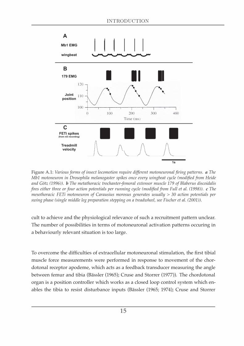
discrepancies between species. Fig. A.1 presents the comparison of motoneuronalfiring patterns of muscles involved in locomotion in three insect species (the fruitflyDrosophila melanogaster, the cockroach Blaberus discoidalis and the stick insect Carausiusmorosus) during physiological movements. Flight muscle b1 depicted in A.1a receivesone action potential per wing stroke, hindleg extensor 179 shown in A.1b is activatedby three or four action potentials per locomotory cycle (during fast running), whereasthe middle leg extensor tibiae shown in A.1c carries out a swing phase with morethan 30 action potentials of the fast motoneuron FETi (mean spike number per burst,see Hooper et al. (2007a)). Each muscle is designed for maximal power and efficiencyin its important range of speed (Full et al. (1998)). The control of activation, i.e. theproperties of force production and contraction related to the motoneuronal spike fre-quency, varies a lot between muscles and suggests their individual twitch-to-tetanusratios to be very different among the three species shown. This ratio represents an es-sential muscle physiological parameter that indicates a muscle´s capacity to finetuneforce and movement. The large differences in activation control between these threeexamplary species highlights the urgency of muscle physiological investigations inthe stick insect.

Hooper and colleagues demonstrated that extensor tibiaemotoneuronal firing is highlyvariable (Hooper et al. (2006)). Measuring this variation on the effector level is theonly way to tell whether this variation is really of physiological relevance for theanimal. Given the well known neural aspects of stick insect leg motor control, under-standing of the FT-joint control would therefore be greatly increased by examiningthe biomechanics of the joint’s muscular system. Conveniently, the extensor tibiaerepresents a very suitable system for the investigation of muscle parameters: it is apinnate muscle whose distal end is easily accessible by opening the femur with a fewcuts and whose innervation is rather simple: one fast and one slow motoneuron (FETiand the SETi; Bässler and Storrer (1980)) and an additional inhibitory common in-hibitor motoneuron (CI1; Bässler et al. (1996); Bässler and Stein (1996)), that run in asingle nerve (nl3, Marquardt (1940)). Its antagonist, the flexor tibiae is very differentin terms of its innervation. It features more than twenty-five excitatory (Goldammeret al. (2007)) and two inhibitory motoneurons (Debrodt and Bässler (1990)) that runin a single nerve as well (ncr, Marquardt (1940)). Especially in the case of the flexortibiae, controlled extracellular stimulation of a particular set of motoneurons is diffi-

14

INTRODUCTION

Figure A.1: Various forms of insect locomotion require different motoneuronal firing patterns. a TheMb1 motoneuron in Drosophila melanogaster spikes once every wingbeat cycle (modified from Heideand Götz (1996)). b The metathoracic trochanter-femoral extensor muscle 179 of Blaberus discoidalisfires either three or four action potentials per running cycle (modified from Full et al. (1998)). c Themesothoracic FETi motoneuron of Carausius morosus generates usually > 30 action potentials perswing phase (single middle leg preparation stepping on a treadwheel, see Fischer et al. (2001)).

cult to achieve and the physiological relevance of such a recruitment pattern unclear.The number of possibilities in terms of motoneuronal activation patterns occuring ina behaviourly relevant situation is too large.

To overcome the difficulties of extracellular motoneuronal stimulation, the first tibialmuscle force measurements were performed in response to movement of the chor-dotonal receptor apodeme, which acts as a feedback transducer measuring the anglebetween femur and tibia (Bässler (1965); Cruse and Storrer (1977)). The chordotonalorgan is a position controller which works as a closed loop control system which en-ables the tibia to resist disturbance inputs (Bässler (1965; 1974); Cruse and Storrer

15

INTRODUCTION

(1977)). Extensor and flexor tibiae act as the actuators within the mechanism, as theirforces try to resist the artificial disturbance input (Cruse and Storrer (1977)). Initialmeasurements were made from the tibia (Bässler (1974)) and later from the extensorand flexor tibiae muscles separately (Storrer (1976); Cruse and Storrer (1977); Bässler(1983)). The reason for the avoidance of extracellular motoneuronal stimulation wasjustified with concerns towards the order of recruitment of extensor tibiae motoneu-rons. FETi has the largest diameter (Bässler and Storrer (1980)) and is therefore thefirst one to be recruited at nl3 stimulation (for a detailed explanation, see Pearsonet al. (1970); Stein and Pearson (1971)). Thus, extracellular SETi stimulation wouldalways involve stimulating FETi as well, which was considered to be too far from aphysiologically interesting situation and left the experimentators unsatisfied at thattime. Consequently, measuring tibial muscle forces and length changes in response todirect motoneuronal stimulation was not taken into account.

However, a simultaneous extracellular stimulation of all extensor motoneurons comesactually quite close to a naturally occuring activation pattern. During walking, FETi,SETi and CI1 are activated maximally during swing phase of the middle leg (Schmitzand Hassfeld (1989); Büschges et al. (1994)). In this context, CI1 activity switches offforce production of dually innervated fibres (Bässler et al. (1996); Bässler and Stein(1996)). Depending on the walking situation, extensor motoneurons can also be ac-tive during stance phase before the initiation of swing, although at a reduced level(Graham (1985); Schmitz and Hassfeld (1989); Büschges et al. (1994)). Simultaneousstimulation of all three extensor tibiae motoneurons via nerve nl3would therefore ab-solutely make sense and was chosen to be the right method to activate the extensortibiae. Hence, by taking benefit of the knowledge available (see above), the middleleg extensor tibiae provides a lot of advantages that make it an ideal muscle physio-logical subject to study, which was done in the thesis at hand.

The muscle investigations presented in the Results section required a careful selectionof the most relevant questions that need to be answered to improve understandingof stick insect walking, as muscle physiology in general is a very broad and com-plex field. It ranges from molecular studies on e.g. ATP-driven Ca2+ -pump (Louet al. (1997)) over force length measurements on highly specialised muscles that canbe stretched nearly three times their resting length (Rose et al. (2001)) to the quantita-

16

INTRODUCTION

tive description of the centre of gravity dynamics during the long jump take-off phasein humans (Seyfarth et al. (1999)). This thesis concentrates on the description of themain basic relationships that generally characterise a muscle and further deals withthe interaction of characteristics and the development of individual parameters in aphysiologically relevant context. The revelation of one of these basic characteristics,the so-called force-length relationship, was closely linked to the progressive explo-ration of structural processes within a sarcomere due to the development of tech-niques like electro microscopy. Those processes are summarised in the term ‘slidingfilament theory´ (Huxley and Niedergerke (1954a); Huxley and Hanson (1954); Pageand Huxley (1963)). A. E. Huxley and H. E. Huxley described the existence of cross-bridges as those structural elements, that are responsible for force generation and forthe sliding of thick and thin filaments (Huxley (1957a;b)). The biochemical processesinvolved were termed ‘power stroke´. Finally, the isometrically developed muscleforces at different fibre lengths could be explained by the number of attached cross-bridges and are described by the sarcomere model (Gordon et al. (1966b)). In order tointerpret this force-length relationship, previous knowledge about the muscle lengthchange within the working range of the limb, which is supposed to be moved, is re-quired (Full et al. (1998)). This additional information is of particular importance asthe muscle experiences length changes during every single contraction. Investigationof pinnate muscles like the extensor and flexor tibiae requires a further determinationof the fibre length, as muscle length and fibre length are not the same, in contrast toparallel fibred muscles like e.g. the human biceps brachiimuscle.

Another important muscle characteristic is the force-velocity relationship, which rep-resents a fundamental property of the contractile system: the ability of a muscle toadjust its force to precisely match the load by varying the speed of shortening appro-priately (Edman et al. (1997)). Fenn andMarsh (Fenn andMarsh (1935)) were the firstto describe this relationship that was a few years later characterised by a rectangularhyperbola (Hill (1938)). This Hill curve defines a muscle´s mechanical capacity - themaximum shortening velocity (V0), the maximum stress (P0) and the expected poweroutput at any load less than P0 or at any shortening velocity between 0 and V0 (Ed-man and Josephson (2007)). Hill provided evidence that muscle shortening involvesheat production, which is due to inner friction that a muscle needs to overcome dur-ing shortening. The heat production by the muscle is proportional to the amount ofshortening, that themuscle experiences. The Hill-equation describes the interrelation-

17

INTRODUCTION

ship between force, velocity and heat (Hill (1938)). Edman mentioned the possibilityto use the force-velocity relationship as a relevant index of muscle activity (Edmanet al. (1997)). Experiments on locust flight muscle (Schistocerca gregaria) showed that itwas indeed possible to derive a so-called ‘degree of activation´ by releasing a muscleat different particular time points during a twitch (Malamud and Josephson (1991)).This is in line with A.V. Hill, who found out that this was a good method to deter-mine when the muscle´s ability to develop work output peaks. Interestingly, this peakarises much earlier than the maximal isometric force output (Hill (1938)). In this con-text, computer models present good means to valuate the importance of a parameterin terms of comparing a situation where this parameter is implemented and anothersituation where it is ommited, as demonstrated by van Soest and Bobbert (van Soestand Bobbert (1993)). They could imposingly show the actual importance of muscle´sforce-length and force-velocity characteristics in a human vertical jumpingmodel andwhich sort of impact those characteristics have to a sudden perturbation. In general,muscle shortening represents a trade-off between the constraints of either movingfast or generating large power output. Elastic elements have the ability to uncouplemuscle fibre shortening velocity from body movement to allow muscle fibres to op-erate more slowly, yet more strongly (Roberts and Marsh (2003)). Investigations onthe plantaris longus muscle in the frog Rana catesbeiana reveals series elasticity to beessential to increase the mechanical work done in order to perform a fast and pow-erful movement at the same time (Roberts and Marsh (2003)). Passive elements likethe series elasticity can have a major impact on locomotion behaviour. In the locust,passive torques have the capacity to lift even a loaded limb without any motoneuronactivity: a large part of flexions and the initiation of extensions were attributable topassive forces (Schistocerca gregaria, Zakotnik et al. (2006)). The distribution of forcesthat arises during limb movement comprises not only the momentum of the actualmass that needs to be accelerated, but also the passive muscle forces of antagonisticmuscle(s) and frictional joint forces, that have to be taken into account. The relevanceof passive muscle forces scales with body size (Hooper et al. (2009)) and represents anessential movement and posture defining parameter in small animals like the stick in-sect. It was shown that loss of motoneuronal innervation in the extensor tibiae can becompensated (to some extent) by an increase in passive static tension, which can leadto a maintenance of walking behaviour (Bässler et al. (2007)). Thus, the knowledgeabout the neuromuscular transform represents only a part of the information that isneeded to understand movement generation. Musculoskeletal units, leg segments,

18

INTRODUCTION

and legs do much of the computations on their own by using segment mass, length,inertia, elasticity, and dampening as ‘primitives´ (Full and Farley (2000)). A mechani-cal system can react much faster to perturbations during rapid, rhythmic activity (Fulland Koditschek (1999)). Nonetheless, passive dynamic control lacks the plasticity ofactive neural control, since suites of integrated structures which have evolved overmillions of years take longer to modify (Full and Farley (2000)).

In addition to the questions that arise around the activation of amuscle and its passivebehaviour, one crucial aspect of the above mentioned musculoskeletal units is theirrelaxation behaviour after active contraction. That is, a muscle can still exert forceeven though motoneuronal firing has ceased. In the isotonic force domain, the stickinsect extensor tibiae takes on average 52 ms after a burst to start relaxing (Hooperet al. (2007a)). This becomes especially functionally relevant at step transitions, whena muscle´s relaxation has not finished and the antagonist muscle is about to be acti-vated. In the stick insect, the transition from swing to stance features co-contraction interms of an extensor and flexor tibiae activity overlap (single leg preparation in Cuni-culina impigra, Fischer et al. (2001)). Antagonistic muscle co-contraction attributable tolong muscle time constants facilitates substantial load compensation (Zakotnik et al.(2006)). The joint stiffness, that results from co-contraction, represents an importantpart of a successful control strategy. The level of co-contraction can vary with thehistory a muscle has experienced in terms of its previous activation or previouslyhappened muscle length changes (see e.g. Ettema and Meijer (2000); Herzog et al.(2003); Ahn et al. (2006)).

The investigations in this thesis are presented and discussed in six chapters respec-tively. The stick insect FT joints of front-, middle- and hindleg were examined in re-spect to their geometrical characteristics. In the middle leg, femur and muscle cross-sectional area, fibre length and sarcomere length were determined for the extensorand flexor tibiae. Experiments determining statically and dynamically generated pas-sive forces and testing creep behaviour were conducted on both tibial muscles of themiddle leg as well. The middle leg extensor tibiae was investigated in respect toits twitch and tetanus kinetics, its relaxation dynamics at different activation levels,its latch properties and its force-length characteristic in the isometric domain. Ex-periments in the isotonic domain included force-velocity measurements at different

19

activation and length levels, the contraction behaviour in response to physiologicalinput and series elasticity measurements at different activation levels. In the finalpart, the interaction of characteristics and the relaxation behaviour were investigatedby mimicking physiologically occuring extensor muscle length changes. Video track-ing of tibial movement should test whether the change in extensor tibiae relaxationdynamics after different activation durations is reflected in tibia movement. Due tothe large amount of motoneurons, active middle leg flexor tibiae measurements wererestricted to quick release experiments including the calculation of the parametersP0 and V0 and series elasticity determinations. These flexor nerve stimulations wereexclusively conducted at maximum activation (i.e. entire motoneuronal recruitmentandmaximum stimulation frequency). The role of FT joint forces alone was examinedby ablating both tibial muscles and deflecting the joint.

Some of the data shown in this thesis (parts of chapters C1, C2, C3, C4 and C5) werealready published in Guschlbauer et al. (2007) (FT joint geometry of all legs, mid-dle leg extensor tibiae single twitch and force-length relationship in terms of activelygenerated isometrical force and passive static tension, extensor tibiae Hill curves atdifferent activation and maximal shotening velocities at different fibre lengths, exten-sor tibiae series elasticity at different activation). Other data shown (a part of chapterC3) are about to be published in parts of Hooper et al. (2009), where I appear as a con-tributing author (extensor and flexor tibiae passive static tension, flexor tibiae dynam-ically generated passive tension, joint deflections either intact, with muscles ablatedor with joint tissue ablated). Some further measurements presented (a part of chapterC4) were the basis for the analysis shown in Hooper et al. (2006; 2007a;b), where I alsoappear as a contributing author (physiological stimulations of the extensor tibiae inthe isotonic force domain).

20

B. Materials and Methods

21

MATERIALS & METHODS

Experiments were carried out on adult female stick insects of the species Carausiusmorosus Br. from a colony maintained at the University of Cologne. Animals werekept under artifical light conditions (12 h darkness, 12 hours light) and were fed withblackberry leaves (Rubus fructiosus). 10 sturdy-looking animals of the same size asused in the experiments had an average body length of 77.1 ± 2.28 mm and averageweight of 940 ± 70 mg. All experiments were performed under daylight conditions(setup light, Olympus) and at room temperature (20-22°C).

1 Femur, muscle, fibre and sarcomere lengthmeasurements

The extensor and flexor tibiae muscles were exposed for length measurements by cut-ting a small window into the proximal and distal part of the femur. The red-colouredautotomal ring (Schindler (1979); Schmidt and Grund (2003)) was assigned as proxi-mal end. Parts of the main leg trachea, the chordotonal organ and the first of three re-tractor unguis muscles (Radnikow and Bässler (1991)) were cut off and highly diluted‘Fast Green´ (Sigma) was applied in most cases. Muscle length was calculated underthe microscope by determining the distance from the insertion of the most proximalfibre to an orientation mark (see Fig. B.1, shown for the extensor tibiae) and addingthe distance from this mark to the insertion of the most distal fibre into the tendon.The animal´s abdomen was stimulated tactilely several times during a test series tomake sure that the investigated muscle was tensed throughout (Bässler and Wegner(1983)). The tibia was moved on a plastic goniometer from 30° (maximally flexed)to 180° (maximally extended) and length measurements were taken in 10° intervals.This range (150°) is considered as the maximum working range of both tibial muscles(Storrer (1976); Cruse and Bartling (1995)). 90° was defined as the FT-joint angle atwhich both muscles are at their resting length for the stick insect (Friedrich (1932);Storrer (1976)) and for Blaberus discoidalis (Full et al. (1998); Ahn and Full (2002)). Fe-mur cross sectional area was detemined by cutting middle legs on the level of themid-coxa. Sections of approximately 1 mm thickness were cut from the medial partof the femur with a razor blade (Rotbart).

22

MATERIALS & METHODS

Fibre length measurements were performed on muscles fixed in situ using 2.5% glu-taraldehyde in phosphate buffer pH 7.4 (Watson and Pflüger (1994)) with the joint atthe 90° position and the entire femur opened laterally. The animal was again stimu-lated tactilely several times during fixation (see above). Fibres were pulled from theproximal and medial parts of the femur because in these locations both muscles areprimarily innervated by fast motoneurons (Bässler et al. (1996); Debrodt and Bässler(1989)). Muscle length changes and fibre length measurements were done using a20x magnifying oculometer (Wild-Heerbrugg) at 25x magnification, femoral lengthwas determined at 6x magnification. Calibration was done with a aluminium-ruler(estimated accuracy of 0.005 mm).

Two different methods were used measuring sarcomere length. In a first approach,middle leg FT-joints were set at angles of 30°, 90°, or 180°. The specimens were fixedin a mixture of 13% formaldehyde/ 59% ethanol/ 6% glacial acetic acid and embed-ded in paraffin. 15µm thick sagittal slices were made and stained with the fast Nisslprocedure (Burck (1988)). Sarcomeres were visualised under a light microscope with apolaroid filter andmeasured with the analySIS software (Soft Imaging System, Olym-pus). The second approach consisted in staining extensor and flexor tibiae muscleswith phalloidin (Phalloidin-FluoProbe 647H 650/670 nm) after fixing the femur as awhole in a mixture of 4% paraformaldehyde in 0.1 M sodium phosphate buffer (pH7.4) and separating the muscles carefully afterwards from the femoral tissue. Phal-loidin was dissolved in 1.5 ml methanol which results in a 6.6 nmol/ml phalloidin so-

proximal endof the femur

proximal end of theextensor tibiae distal end of

the femurorientation mark

30°

90°

180°

TrochanterCoxa

Femur

Tibia

Figure B.1: Schematic representation of the geometrical arrangement of the femur-tibia joint in thestick insect middle leg. See text for details.

23

MATERIALS & METHODS

lution. 7.5µl of this solution were mixed with 400µl phosphate buffered saline (PBS).Muscles were incubated in a mixture of 0.16 nmolml phalloidin solution with 1% Triton-X in PBS for 15min (modified from Thuma (2007)). Concentrations of 0.32 nmolml and0.08 nmol

ml were tested as well and led to worse results. Phalloidin stained sarcomerelengths were first measured at the actual contraction state when being fixed, that is at30° and 180° FT-joint angle. Then, sarcomere lengths were determined by standardis-ation according to the instructions suggested by Thuma (2007), see Fig. B.2. The goalof such a normalisation procedure is to specify lengths independent from contractionstate, because different muscles are known to have different sarcomere lengths. Thecomparison of sarcomere lengths between muscles therefore necessitates the reduc-tion of a sarcomere to its own physical characteristics. This reduction provides anunambigious anatomical base to determine sarcomere length independent from con-traction state, because the standardised sarcomere length measures two times thinfilament length.

Figure B.2: Standardisation of sarcomere length. Sarcomere lengths from the same type of muscle differbecause of different muscle contraction states. To correct this, a standardisation protocol can be appliedto each sarcomere length (modified after Thuma (2007)).

24

MATERIALS & METHODS

2 Measurements with the Aurora 300B dual modelever system

The ‘Aurora 300B dual mode lever system´ (Aurora Scientific Inc, Ontario, Canada) isa device enabling to measure and control both force and position simultaneously andto make the transition from force to position control with only small transients (Fig.B.3 shows a picture of the device). Forces of maximally 500 mN and length excursionsof maximally 10 mm can be detected with a force signal resolution of 0.3 mN and alength signal resolution of 1 micron. Force step and length step response time are 1.3ms and 1 ms respectively. It acts like a length controller that is precision force-limitedand acts exclusively as a force controller if an external load attempts to pull harderthan the set force level. Its servo motor has a preferred direction of force applicationalthough forces can be measured in both directions. Load should be attached to thelever arm such that a muscle contraction will pull the lever arm in a counterclockwisedirection (when viewed from the shaft end of the motor).

The lever arm of the Aurora servo motor is 30 mm long and perforated at the tip.Its connection to a muscle is the combination of an u-shaped pin being glued to acut thick insect pin being in turn glued to a 0.1 mm thin hook-shaped insect pin. Afew experiments were done using a sterile silk thread (50 µm; Resorbi, Nürnberg) incombination with a hook-shaped insect pin as link between lever arm and muscle.Force and position measurements with the lever system were mainly made on theextensor tibiae muscle of the middle leg, some experiments dealt with the flexor tibiaemuscle´s properties. The lever system was tuned so that length control was criticallydamped and inertia compensation was adjusted to minimise force transients usingtriangle waveforms as suggested in the Aurora´s instruction manual.

For investigation of FT joint torques, a special lever arm was built (mechanics depart-ment of the Zoological institute, University of Cologne). Its effective moment armlength is 4.75 mm. The lever arm that was usually used narrows to the perforated tipand has an effective moment arm of 30 mm. Amiddle leg was cut on level of the mid-coxa andwas fixed on the platform and positioned such that its FT joint rotational axisand its pivot was the same as the servo motor´s. A plastic rod formed the connectionbetween the lever arm and the tibia, with which it could be easily attached because

25

MATERIALS & METHODS

Figure B.3: The Aurora dual-mode lever arm system 300B (Aurora Scientific Inc.). The picture showsonly the main device, i.e. the controller, not the servo motor.

of a notch that was sligthly narrower than the average stick insect tibia (see Fig. B.4).Additionally, a drop of super glue (Loctite, Uhu Alleskleber) assured a good bondbetween tibia and the notch in the plastic rod. Finally, apodemes of both extensor andflexor tibiae were cut through the soft cuticle at the anatomical transition from femurto tibia with fine scissors.

ac

b

Figure B.4:Measuring FT-joint torques with a specialised device. a tibia, b femur embedded in dentalcement, c modified lever arm (the lever arm that was usually used is depicted in Fig. B.7).

26

MATERIALS & METHODS

3 Animal preparation and dissection

All legs except one middle leg were cut at the level of the mid-coxa. The animal wastreated according to the established procedures and was fixed dorsal side up on abalsa wood platform so that the tibia of the remaining leg was suspended above theedge of the platform in all extensor tibiae investigations. The tibia had to be cut inall flexor tibiae experiments. Coxa, trochanter, and femur were glued to the platformwith dental cement (Protemp II, ESPE, St. Paul, MN, USA). The distal end of the femurwas opened carefully to ensure that as many muscle fibres were left intact as possible.The femoral cavity was filledwith ringer (NaCl 178.54mM,HEPES 10mM, CaCl2 7.51mM, KCl 17.61 mM, MgCl2 25 mM) (Weidler and Diecke (1969)) several times duringeach experiment (see also Becht et al. (1960)). Muscle investigations were achieved byinserting the hook-shaped insect pin (described above) through the cut distal end ofeither the extensor or flexor tibiae distal muscle apodeme (see also Ahn et al. (2006)).Cutting of the apodeme was conducted under controlled conditions: muscle lengthwas set to its corresponding length at a FT-joint angle of 90° at the beginning of eachmeasurement. Flexor tibiae muscles were normally that strong that the hook-shapedpin had to be glued (Loctite 401, Uhu Alleskleber Super) to the apodeme in additionto the insertion through the tendon.

4 Extracellular motoneuronal recording

Nerves F2 and nl3, both containing the three extensor tibiaemotoaxons, were recordedin different experiments en passant (Schmitz et al. (1991)) with a monopolar hook elec-trode filled with silicone paste (high-viscosity, Bayer), modified by the mechanics de-partment of the Zoological institute, University of Cologne. A fine polyethylene tubecan be slided on the nerve, which can in turn be isolated with the silicone paste. Asilver wire (0.25 mm in width) served as a reference electrode. The signal was eitherpreampedwith a battery-powered optocoupler (100x) or by a ‘Ultra low noise pream-plifierMA103´ (50x), boosted by an AC-filter amplifier (20x or 50x) and sampled by anAD-converter (Cambridge Electronics 1401) with 12500 Hz. The filter range settingsof the booster were usually 150 Hz-9500 Hz.

Nerve activity could be made audible by a monitor (1278), that was amplified with aDC filter amplifier (1274A). All devices were built in the electronics department of the

27

MATERIALS & METHODS

Zoological insitute of the University of Cologne when not noted differently.

5 Electrical stimulation of motoaxons

5.1 Recruitment of extensor tibiae motoneurons

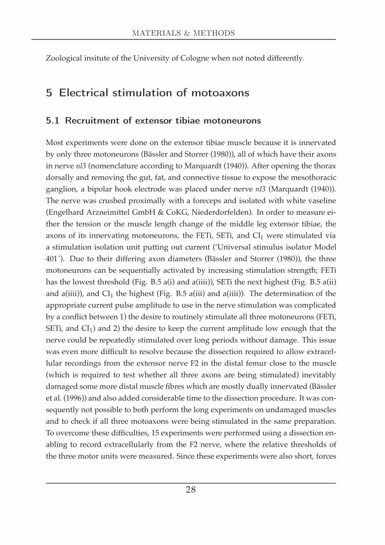
Most experiments were done on the extensor tibiae muscle because it is innervatedby only three motoneurons (Bässler and Storrer (1980)), all of which have their axonsin nerve nl3 (nomenclature according to Marquardt (1940)). After opening the thoraxdorsally and removing the gut, fat, and connective tissue to expose the mesothoracicganglion, a bipolar hook electrode was placed under nerve nl3 (Marquardt (1940)).The nerve was crushed proximally with a foreceps and isolated with white vaseline(Engelhard Arzneimittel GmbH & CoKG, Niederdorfelden). In order to measure ei-ther the tension or the muscle length change of the middle leg extensor tibiae, theaxons of its innervating motoneurons, the FETi, SETi, and CI1 were stimulated viaa stimulation isolation unit putting out current (‘Universal stimulus isolator Model401´). Due to their differing axon diameters (Bässler and Storrer (1980)), the threemotoneurons can be sequentially activated by increasing stimulation strength; FETihas the lowest threshold (Fig. B.5 a(i) and a(iiii)), SETi the next highest (Fig. B.5 a(ii)and a(iiii)), and CI1 the highest (Fig. B.5 a(iii) and a(iiii)). The determination of theappropriate current pulse amplitude to use in the nerve stimulation was complicatedby a conflict between 1) the desire to routinely stimulate all three motoneurons (FETi,SETi, and CI1) and 2) the desire to keep the current amplitude low enough that thenerve could be repeatedly stimulated over long periods without damage. This issuewas even more difficult to resolve because the dissection required to allow extracel-lular recordings from the extensor nerve F2 in the distal femur close to the muscle(which is required to test whether all three axons are being stimulated) inevitablydamaged some more distal muscle fibres which are mostly dually innervated (Bässleret al. (1996)) and also added considerable time to the dissection procedure. It was con-sequently not possible to both perform the long experiments on undamaged musclesand to check if all three motoaxons were being stimulated in the same preparation.To overcome these difficulties, 15 experiments were performed using a dissection en-abling to record extracellularly from the F2 nerve, where the relative thresholds ofthe three motor units were measured. Since these experiments were also short, forces

28

MATERIALS & METHODS

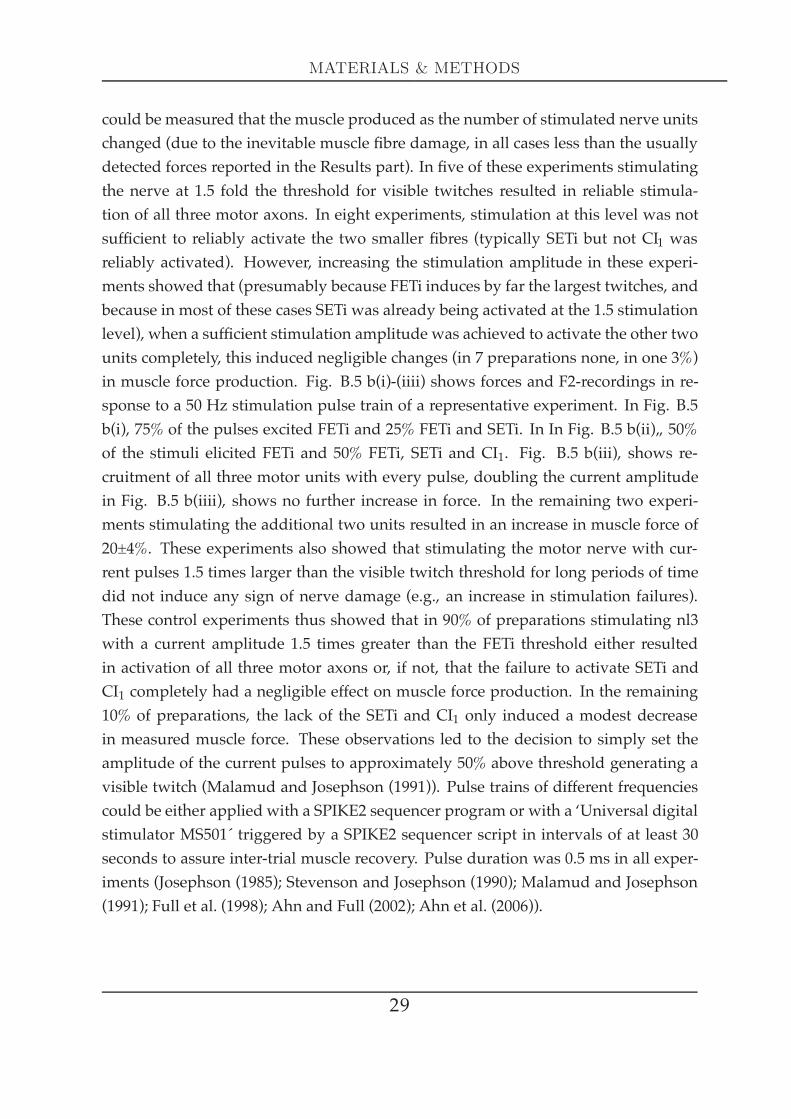
could be measured that the muscle produced as the number of stimulated nerve unitschanged (due to the inevitable muscle fibre damage, in all cases less than the usuallydetected forces reported in the Results part). In five of these experiments stimulatingthe nerve at 1.5 fold the threshold for visible twitches resulted in reliable stimula-tion of all three motor axons. In eight experiments, stimulation at this level was notsufficient to reliably activate the two smaller fibres (typically SETi but not CI1 wasreliably activated). However, increasing the stimulation amplitude in these experi-ments showed that (presumably because FETi induces by far the largest twitches, andbecause in most of these cases SETi was already being activated at the 1.5 stimulationlevel), when a sufficient stimulation amplitude was achieved to activate the other twounits completely, this induced negligible changes (in 7 preparations none, in one 3%)in muscle force production. Fig. B.5 b(i)-(iiii) shows forces and F2-recordings in re-sponse to a 50 Hz stimulation pulse train of a representative experiment. In Fig. B.5b(i), 75% of the pulses excited FETi and 25% FETi and SETi. In In Fig. B.5 b(ii)„ 50%of the stimuli elicited FETi and 50% FETi, SETi and CI1. Fig. B.5 b(iii), shows re-cruitment of all three motor units with every pulse, doubling the current amplitudein Fig. B.5 b(iiii), shows no further increase in force. In the remaining two experi-ments stimulating the additional two units resulted in an increase in muscle force of20±4%. These experiments also showed that stimulating the motor nerve with cur-rent pulses 1.5 times larger than the visible twitch threshold for long periods of timedid not induce any sign of nerve damage (e.g., an increase in stimulation failures).These control experiments thus showed that in 90% of preparations stimulating nl3with a current amplitude 1.5 times greater than the FETi threshold either resultedin activation of all three motor axons or, if not, that the failure to activate SETi andCI1 completely had a negligible effect on muscle force production. In the remaining10% of preparations, the lack of the SETi and CI1 only induced a modest decreasein measured muscle force. These observations led to the decision to simply set theamplitude of the current pulses to approximately 50% above threshold generating avisible twitch (Malamud and Josephson (1991)). Pulse trains of different frequenciescould be either applied with a SPIKE2 sequencer program or with a ‘Universal digitalstimulator MS501´ triggered by a SPIKE2 sequencer script in intervals of at least 30seconds to assure inter-trial muscle recovery. Pulse duration was 0.5 ms in all exper-iments (Josephson (1985); Stevenson and Josephson (1990); Malamud and Josephson(1991); Full et al. (1998); Ahn and Full (2002); Ahn et al. (2006)).

29

MATERIALS & METHODS

FETistimulus artefact

1 T

1.78 T

2.67 T

5.33 T

1.33 TFETi, SETi

1.78 TFETi, SETi, CI1

1.5 Ta(i) b(i)

a(ii) b(ii)

a(iii) b(iii)

a(iiii) b(iiii)

50 ms

0.5 mN

100 ms

10 mN

*

**

***

5 ms

* ** ***

Figure B.5: Isometric forces induced in the middle leg extensor tibiae muscle by electrical stimula-tion of nerve nl3 with different current amplitudes. In all panels the top trace is a stimulus monitor(note pulse height changes as stimulus amplitude was increased), the second trace is an extracellularrecording of nerve nl3, and the third trace is muscle force. a(i)-a(iii) show sequential recruitment ofFETi (a(i)), FETi and SETi (a(ii)) and FETi, SETi and CI1 (a(iii)) recorded in extensor leg nerve F2in response to single stimuli. a(iiii): An enlarged version of the recordings showing the sequentialaddition of new units. 1 T was 0.0023 mA. b(i)-b(iiii) show F2-recordings and forces in response toa 50 Hz pulse train. In b(i), 75% of the pulses excited FETi and 25% FETi and SETi. In b(ii), 50%of the stimuli elicited FETi and 50% FETi, SETi and CI1. b(iii) shows recruitment of all three motorunits with every pulse. Doubling the current amplitude (b(iiii)) induced no further increase in force.In this experiment the SETi spikes were of larger amplitude than FETi spikes. This is uncommon andlikely because nerve F2 was recorded very distally in the femur. In all panels the electrical disturbancein the nerve recording that coincides with the stimulus is a stimulus artifact, not an action potential(arrow in a(i)).

30

MATERIALS & METHODS

Figs. B.6 (scheme) and B.7 (photograph) summarise the above described. All experi-ments examining muscle force were based on this setup configuration.

PositionOFFSET OUTIN

ForceOFFSET OUTIN

Current

a b

c

de

f

g

Figure B.6: Experimental overview. a Computer, b AD-converter, c stimulation isolation unit, dbipolar electrode on either nerve nl3 (extensor tibiae stimulation) or ncr (flexor tibiae stimulation), emonopolar recording electrode on nerve F2, f Aurora servo motor, g Aurora control device.

31

MATERIALS & METHODS

a bc

d

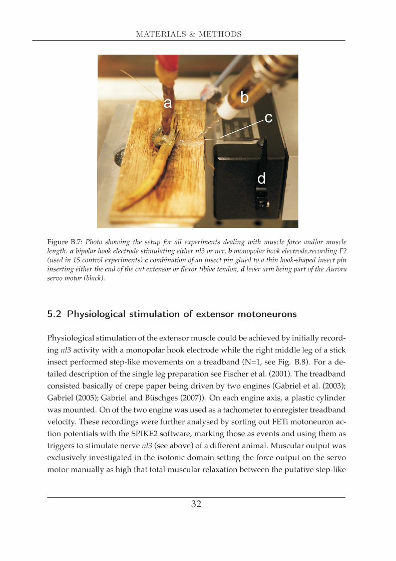
Figure B.7: Photo showing the setup for all experiments dealing with muscle force and/or musclelength. a bipolar hook electrode stimulating either nl3 or ncr, b monopolar hook electrode,recording F2(used in 15 control experiments) c combination of an insect pin glued to a thin hook-shaped insect pininserting either the end of the cut extensor or flexor tibiae tendon, d lever arm being part of the Auroraservo motor (black).

5.2 Physiological stimulation of extensor motoneurons

Physiological stimulation of the extensor muscle could be achieved by initially record-ing nl3 activity with a monopolar hook electrode while the right middle leg of a stickinsect performed step-like movements on a treadband (N=1, see Fig. B.8). For a de-tailed description of the single leg preparation see Fischer et al. (2001). The treadbandconsisted basically of crepe paper being driven by two engines (Gabriel et al. (2003);Gabriel (2005); Gabriel and Büschges (2007)). On each engine axis, a plastic cylinderwas mounted. On of the two engine was used as a tachometer to enregister treadbandvelocity. These recordings were further analysed by sorting out FETi motoneuron ac-tion potentials with the SPIKE2 software, marking those as events and using them astriggers to stimulate nerve nl3 (see above) of a different animal. Muscular output wasexclusively investigated in the isotonic domain setting the force output on the servomotor manually as high that total muscular relaxation between the putative step-like

32

MATERIALS & METHODS

movements (visible as contractions) could be accomplished.

7.4cm/s

1 s

nl3activity

Treadwheelvelocity

Figure B.8: Recorded extensor nerve (nl3) activity while a stick insect performed step-like movementson the treadwheel shown in the lower trace (for a detailed description of the single leg preparation, seeFischer et al. (2001)). Velocity of the treadwheel´s tachometer is displayed in the upper trace.

5.3 Stimulation of flexor tibiae motoneurons

The flexor tibiae muscle is innervated by about 14 motoneurons running in nervencr (Storrer et al. (1986); Debrodt and Bässler (1989); Gabriel et al. (2003)). Recentinvestigations resulted in an even larger number of flexor tibiae motoneurons (18-27, N=8; Goldammer et al. (2007)). Thus, extracellular stimulation of this muscleis complicated to achieve, therefore only a few experimental paradigms carried outon the extensor tibiae were conducted on the flexor tibiae as well. A bipolar hookelectrode was placed under nerve ncr, crushed proximally and isolated with vaseline(as described for nerve nl3). At the beginning of each experiment in the isotonic forcedomain, stimulation amplitude was increased until isometric force showed no furtherincrease and force development showed no visible stimulation failure. Sequentialrecruitment was mainly tested investigating single twitches. As maximal output bythe MICRO1401 A/D converter (Cambridge Electronic Design Limited; Cambridge,UK) was limited to 5 V (i.e. maximally 250mN force application on the Aurora´s leverarm), the force output was amplified with an amplifier / signal conditioner MA102by factor 2 (500 mN is the Aurora´s maximal measuring capacity). Detected flexortibiae forces were not exceeding this value.

5.4 Isometric force experiments

Experiments to determine the active and passive force-length characteristics accord-ing to Gordon and colleagues (Gordon et al. (1966b)) were carried out as follows:

33

MATERIALS & METHODS

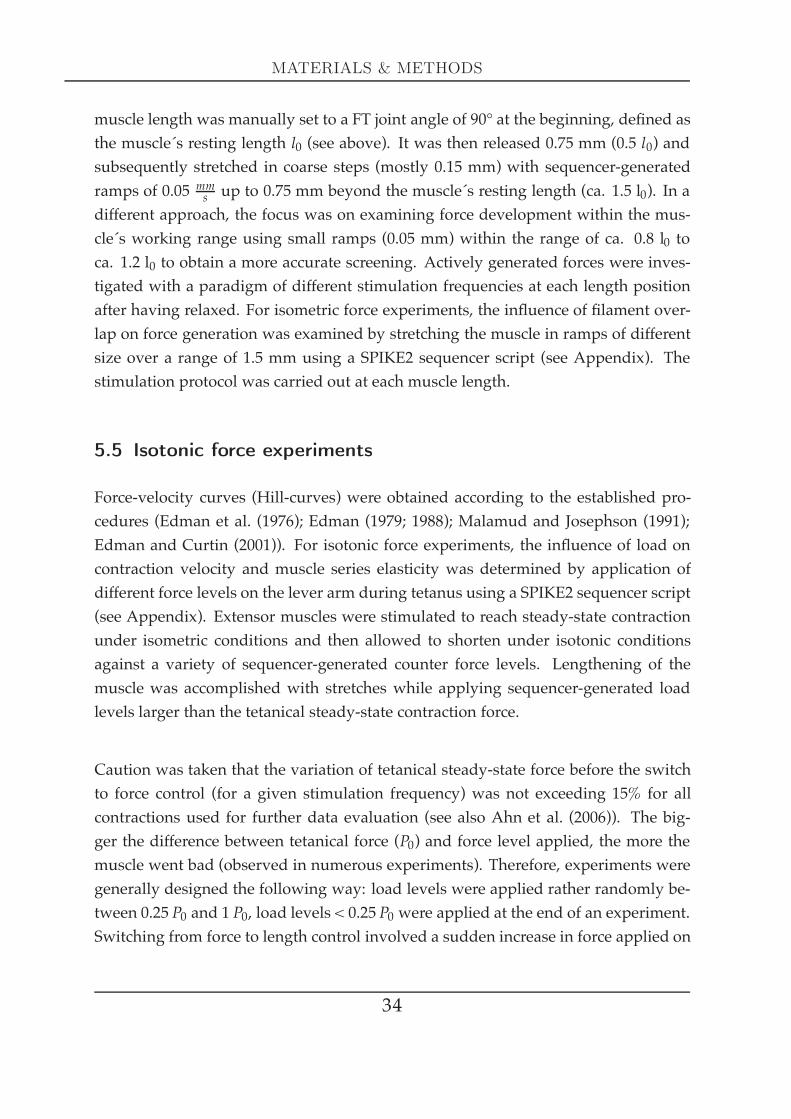
muscle length was manually set to a FT joint angle of 90° at the beginning, defined asthe muscle´s resting length l0 (see above). It was then released 0.75 mm (0.5 l0) andsubsequently stretched in coarse steps (mostly 0.15 mm) with sequencer-generatedramps of 0.05 mms up to 0.75 mm beyond the muscle´s resting length (ca. 1.5 l0). In adifferent approach, the focus was on examining force development within the mus-cle´s working range using small ramps (0.05 mm) within the range of ca. 0.8 l0 toca. 1.2 l0 to obtain a more accurate screening. Actively generated forces were inves-tigated with a paradigm of different stimulation frequencies at each length positionafter having relaxed. For isometric force experiments, the influence of filament over-lap on force generation was examined by stretching the muscle in ramps of differentsize over a range of 1.5 mm using a SPIKE2 sequencer script (see Appendix). Thestimulation protocol was carried out at each muscle length.

5.5 Isotonic force experiments

Force-velocity curves (Hill-curves) were obtained according to the established pro-cedures (Edman et al. (1976); Edman (1979; 1988); Malamud and Josephson (1991);Edman and Curtin (2001)). For isotonic force experiments, the influence of load oncontraction velocity and muscle series elasticity was determined by application ofdifferent force levels on the lever arm during tetanus using a SPIKE2 sequencer script(see Appendix). Extensor muscles were stimulated to reach steady-state contractionunder isometric conditions and then allowed to shorten under isotonic conditionsagainst a variety of sequencer-generated counter force levels. Lengthening of themuscle was accomplished with stretches while applying sequencer-generated loadlevels larger than the tetanical steady-state contraction force.

Caution was taken that the variation of tetanical steady-state force before the switchto force control (for a given stimulation frequency) was not exceeding 15% for allcontractions used for further data evaluation (see also Ahn et al. (2006)). The big-ger the difference between tetanical force (P0) and force level applied, the more themuscle went bad (observed in numerous experiments). Therefore, experiments weregenerally designed the following way: load levels were applied rather randomly be-tween 0.25 P0 and 1 P0, load levels < 0.25 P0 were applied at the end of an experiment.Switching from force to length control involved a sudden increase in force applied on

34

MATERIALS & METHODS

the lever arm. This abrupt step was most often filtered with an ‘amplifier / signalconditioner MA102´ or a ‘DC filter amplifier 1274A´.

6 Photo and video tracking of tibia movements

Movement still photographs of the FT joint were taken in two different ways. Passivemovements were tracked by pinching cut middle legs horizontally into a clamp (with-out gravitational effects). A digital camera (Fuji FinePix S602) was placed on a tripodabove the leg´s FT joint. Pictures were evaluated using the CorelDRAW software:cursors could be tilted to the desired angle in order to lay on top of the tibia picture infocus with an estimated accuracy of 1°. Muscles were ablated by cutting the tendonat the most distal part of the femur without previous dissection, the transitional partfrom femur to tibia has a very thin cuticle and is well accessible.

Tibia movement dynamics were tracked using a VGA highspeed camera (‘AVT Mar-lin F-033C´) and pictures were taken in 10 ms intervals. Nerve stimulation (200 Hzpulses) of either nl3 (extensor tibiae) or ncr (flexor tibiae) and video tracking were trig-gered by a ‘Universal Digital Stimulator MS501´. The antagonistic nerve (either nl3 orncr) was crushed or cut to avoid reflex behaviour (Bässler and Büschges (1998)). Eachframe was triggered individually by a 100Hz pulse train that was gated manually.Nerve stimulation started with a 50 ms delay to have at least 5 single pictures of thenon-moving tibia as a reference point. Pictures were evaluated in CorelDRAW in thesame way described for the photos taken with the digital camera ‘Fuji FinePix S602´(see Fig. B.9).

Figure B.9: (a) Single still photographs of a tibia movement high-speed video track with the FT-jointhighlighted with red lines at the leftmost picture. The example shows stimulation with 80 spikes.Angular evaluation of the asterisk marked picture is displayed in (b): FT joint angle was measured bysetting cursors in the CorelDRAW software.

35

MATERIALS & METHODS

7 Data achievement, storage and evaluation

Data was recorded on a PC using aMICRO1401A/D converter with SPIKE2-software(both Cambridge Electronic Design Limited; Cambridge, UK). The stiffness of themeasuring system was measured by connecting the insect pin directly to the base ofthe platform. It was greater than 7500 mNmm and can therefore be neglected in our mea-surements. Jewell andWilkie discuss the influence of the compliance of themeasuringdevice thoroughly (Jewell and Wilkie (1958)). For most of the data analysis, customSPIKE2 script programs were written (see Appendix). Plotting, curve fitting, and er-ror evaluation were performed in ORIGIN 6.0 (Microcal. Software Inc, Northampton,MA, USA) except for the RC-type growth and exponential decay fits performed inGNUPLOT. This PhD-thesis was written with the LYX/LATEX software.

7.1 Statistics

Mean values were compared using ORIGIN´s

either unpaired

t = (x1−x2−d0)√s2( 1n1+ 1

n2)

or paired

t =D−d0SD

two sample t-test.

(xn is mean of samplegroup n, d0 is a specific value, s is the S.D., nn is number ofsamplegroup n, D is the mean difference.)

Regression analysis was used to determine linear correlation between two variables.The ORIGIN 6.0 software used the least squares method to calculate the slope andprovided the correlation coefficient (R value) and the p-value (probability, that R=0).Means, samples and correlation coefficients were regarded as significantly differentfrom zero or each other at p < 0.05. The following symbols show the level of statistical

36

significance: (-) not significant; (*) 0.01≤ p< 0.05; (**) 0.001≤ p< 0.01; (***) p< 0.001.In the text, N gives the number of experiments or animals while n gives the samplesize. All data were calculated as mean ± S.D. R-values or R2-values are specifiedadditionally when it was reasonable.

37

C. Results

38

RESULTS

C1 Femoral geometry

The ‘Results´ part is generally structured in the following way: the majority of thethesis´ topics were examined on the extensor tibiae of the middle leg, some of thosetopics were also examined on the flexor tibiae of the middle leg. Muscle data is there-fore presented first for the extensor tibiae and subsequently for the flexor tibiae whenever there was data collected. Front, middle and hind leg data are presented, whenavailable, for both muscles when indicated.

1 Muscle length measurements of front, middle andhind leg tibial muscles

1.1 Relationship between resting muscle length and femur length

Resting muscle length was measured (at 90° joint angle, see ‘Materials and Methods´)of flexor and extensor tibiae for the front (flexor N=3, extensor N=3), middle (flexorN=5, extensor N=8) and hind legs (flexor N=3, extensor N=3, Fig. C.1). The linearregression of this data showed in 5 cases a significant dependence of muscle lengthon femur length (*, p < 0.05 or better), only the flexor tibiae front leg data showedno significant dependence. The dependence was simplifed in Fig. C.1 for all legs to apure proportionality forcing the regression lines through the origin (dotted lines, seealso Tab. C.1). For comparison, the 1:1 proportion (solid line) is included.

39

FEMORAL GEOMETRY

0 4 8 12 160

4

8

12

16

Femur length [mm]

Musc

lere

stin

gle

ngth

[mm

]

F

HM

F

HM

flexor

extensor

Figure C.1: Relationship between muscle resting length and femur length in front leg (squares), mid-dle leg (circles) and hind leg (triangles). Data points for the extensor tibiae are represented by filledsymbols, data points for flexor tibiae are represented by open symbols. The dotted lines give the lin-ear fit under the assumption of pure proportionality between muscle length and femur length. Forcomparision the 1:1 proportion is added as a solid line. Values are shown in Tab. C.1.

Table C.1: Relationship between muscle length and femur length. Mean percentages arise from theslopes of linear fits forced through the origin (all significant, * (p < 0.05 or better) with the exceptionof flexor tibiae front leg data not being significant (-).

Percentage of femur length NExtensor tibiae FL ! 75.7± 0.6 3Extensor tibiae ML • 90.1±0.9 8Extensor tibiae HL " 89.7±0.7 3Flexor tibiae FL # 72.7±2.5 3Flexor tibiae ML ◦ 94±0.2 5Flexor tibiae HL $ 95.4±0 3

1.2 Relationship between muscle length and FT-joint angle

From the resting position of 90°, the length change of the tibial muscles as a functionof FT-joint angle was investigated. Given a fixed moment arm length of H, the length

40

RESULTS

change should have the form of x = H · cos(α), where α is FT joint angle. Fig. C.2shows the normalised data compared to the cosine function. For the extensor musclechanges in joint angle depend on +cos(α), for the flexor muscle on −cos(α) (the signdifference arises from the fact that extension shortens the extensor muscle and length-ens the flexor tibiae). Normalised datapoints show good accordance with the addi-tionally displayes cosine function within a range from 50-160°. At extreme FT jointangles (< 50° and > 160°), datapoints tend to deviate slightly from the cosine function,which makes sense in respect to tibia movement mechanics (see ‘Discussion´).

1.3 Moment arm determination

The slope of the plots of muscle length versus cos(α) is equivalent to the momentarm, because of moment arm length = ∆muscle length

cos(α) . Fig. C.3 shows that the flexor

-1.0

-0.5

0.0

0.5

1.0

FT-joint angle [°]

Norm

alis

ed

musc

lele

ngth

change

0 30 60 120 150 18090 0 30 60 120 150 18090

0 30 60 120 150 18090 0 30 60 120 150 18090

-1.0

-0.5

0.0

0.5

1.0

FT-joint angle [°]

middle leg extensor middle leg flexor

-1.0

-0.5

0.0

0.5

1.0

FT-joint angle [°]

hind leg extensor

-1.0

-0.5

0.0

0.5

1.0

FT-joint angle [°]

Norm

alis

ed

musc

lele

ngth

change

front leg extensor

Figure C.2:Normalised muscle length change as a function of FT-joint angle. Extensor data are showncompared with +cos(α) flexor data are compared with −cos(α) (solid lines).

41

FEMORAL GEOMETRY

muscle moment arms of all leg joints are about two times larger than the extensormuscle moment arms (mean flexor moment arm length, 0.56 ± 0.04 mm, N=7 andmean extensor moment arm length 0.28 ± 0.02 mm, N=7).

2 Fibre length measurements of middle leg tibialmuscles

As in all orthopteran legs, both the extensor and flexor tibae of the stick insect arepinnate muscles (Storrer (1976)). This fibre arrangement markedly presents an ad-vantage in terms of effective muscle cross-sectional area and maximum muscle force(Hildebrand (1988)) but decreases effective muscle length and maximum contractionvelocity. Given a mean fibre diameter of 0.125 mm (Bässler and Storrer (1980)), anda mean of 156 fibres per muscle (N=4; min. n=146, max. n=172) an estimated meancross-sectional area of the extensor tibiae muscle is 1.91 mm². As the extensor tibiaefills out about the upper third of the femur (3D-reconstruction model of Ulrich Bässler;Bässler et al. (1996)), the lower two thirds of the femur can be attributed to the flexor

0 4 8 12 16 200.0

0.2

0.4

0.6

Femur length [mm]

Mom

entarm

length

[mm

]

F

HM

flexor

extensor

Figure C.3: Relation between femur-tibia joint moment arm and femur length. Note that moment armdoes not depend on femur length. Closed symbols are data from extensor muscles from 2 front legs(squares), 2 hind legs (triangles), and 3 middle legs (circles), while open symbols are data for flexortibiae muscles from 5 middle legs (circles) and two front legs (triangles).

42

RESULTS

tibiae, which is therefore estimated to have a cross-sectional area of 4 mm². For pin-nate muscles, length changes of the muscle as a whole do not lead to the same changesin muscle fibre length; muscle fibre length instead varies with muscle length times thecosine of the pinnation angle, which in return varies as muscle length changes. Forthe extensor tibiae, a range of angles from 8.2 - 12° for the proximal and 10.2 - 15.6°for the medial fibres can be found within physiological muscle lengths. For the flexortibiae, a range of 11.1 - 12.9° for the proximal and 12.4 - 15.4° for the medial part of thefibres can be determined. These calculations are based on the determination of fibrelength (see next paragraph) and the distance from the tendon to the cuticle (where thefibres are attached). Calculation of errors was conducted using Pythagoras´ law: thecosine correction was only 3.7% for the extensor and 2.9% for the flexor tibiae for thelargest angle, so a correction can be neglected (i.e. the muscle fibres were treated asthough they were arranged parallel to the muscle longitudinal axis in both cases).

The analysis of the relation between fibre length and muscle length is depicted inFig. C.4. Proximal fibres of the extensor tibiae muscle had a mean length of 1.47 ±0.21 mm (N=5) and are about 0.13 mm longer than the medial muscle fibres (N=5).From these results, a mean fibre length of the extensor tibiae was 1.41 ± 0.23 mm. Incontrast, flexor tibiae proximal fibres had a mean length of 2.0 ± 0.32 mm (N=4) andare about 0.21 mm shorter than the medial fibres (N=4). The mean fibre length of theflexor tibiae is therefore 2.11 ± 0.30 mm. Regression analysis of this data showed asignificant linear dependence of fibre length on extensor muscle length (*, p ≤ 0.03),whereas no such dependence was detected for flexor tibiae muscle fibres (see dottedregression lines).

3 Sarcomere length measurements of middle legtibial muscles

The following data set on sarcomere length represents a preliminary version, the in-vestigation is not finalised yet. Because of sarcomeres being the fundamental func-tional units that a muscle consists of, an initial characterisation was carried out thatis supposed to prompt future work. The ultimate goal of these examinations was to

43

FEMORAL GEOMETRY

0 2 4 6 8 100.0

1.0

2.0

extensor

Muscle resting length [mm]

proximalmedial

flexor

Fib

rele

ng

th[m

m]

Figure C.4: Relation between middle leg muscle resting length and fibre length. Extensor muscle fibrelength depends on muscle resting length (*, p ≤ 0.03), whereas no such dependence is present in theflexor muscle (-, p ≥ 0.05, dotted regression lines). Open circles denote data from medial muscle fibres,filled circles from proximal ones. Data are means ± S.D. from nine animals (N=9).

relate a gross leg property (i.e. the joint angle) to a microscopic muscle property (i.e.the sarcomere length). The relevant question was as follows: Does the percent lengthchange that extensor and flexor tibiae fibres experiencewithin the physiological work-ing range of 150° match the percent length change that the sarcomeres of these fibresexperience? It was first attempted to measure sarcomere length with the muscle fibresbeing fast Nissl stained (Burck (1988)). Proximal and medial parts of the extensor andflexor tibiae fibres were investigated because of being predominately innervated byfast motoneurons (Debrodt and Bässler (1989); Bässler et al. (1996)). The study wasnot satisfactory, as only the dark A-bands (overlap of thick and thin filaments) andthe much brighter I-bands (only thin filaments with the Z-lines in between) could bedistinguished. The treatment that was necessary for the fast Nissl stainings involveddrying, paraffin embedding and sectioning into 15 µm slices (see ‘Materials and Meth-ods´ section). It is very likely that this whole procedure led to deformations of thestained sarcomeres. Hence, the method was considered to be inappropriate becausethe visibility of structures was limited and analysis of the stained material was ques-tionable.

Further stainings were accomplished. Phalloidin stains F-Actin (Thuma (2007)) andis easier to handle because it does not require sectioning of the specimen and fibres

44

RESULTS

can be directly scanned on the Laser ScanningMicroscope (LSM). Phalloidin stainingshave a much greater visibility and therefore allow the discrimination of Z lines, thinfilament overlap and H-Bands, see Fig. C.5a-c.

Measurements were taken from extensor and flexor tibiae fibres at 30° and 180° FTjoint angle (see Fig. C.6a(i), a(ii), b(i), b(ii) and Tab. C.2). Extensor tibiae sarcomereshave a length of 7.50 ± 0.75 µm (N=1, n=114) at 30° and a length of 6.21 ± 0.38 µm(N=1, n=97) at 180°. Flexor tibiae sarcomeres have a length of 5.16 ± 0.16 µm (N=1,n=60) at 30° and a length of 9.16 ± 0.46 µm (N=1, n=31) at 180°. For extensor tibiaefibres, the ratio Fl at 30 deg

Fl at 180 deg is 1.46 (calculated with a mean fibre length of 1.41 mm at90° FT joint angle and a mean moment arm length of 0.282 mm) and the correspond-ing ratio for the sarcomeres Sl at 30 deg

Sl at 180 deg is 1.21: sarcomeres experience 25 % less relativelength change than fibres. For flexor tibiae fibres, the ratio Fl at 180 deg

Fl at 30 deg is 1.65 (calcu-lated with a mean fibre length of 2.11 mm at 90° FT joint angle and a mean momentarm length of 0.564 mm) and the corresponding ratio for the sarcomeres Sl at 180 degSl at 30 deg is1.78: sarcomeres experience 13 % more relative length change than fibres. The lengthchanges of the fibre do not match the sarcomere length changes, but the calculatedvalues are close enough to make the conclusion that there is a gross correlation be-tween fibre and sarcomere length changes. The results suggest that there might bemuscle properties (e.g. cuticle or tendon proteins) that involve processes that couldlead to the calculated mismatches. Further examinations should clarify whether thismismatch is detectable in more muscles.

Figure C.5: LSM (laser scanning microscope) pictures showing either thin filament overlap (a, b) oroccurence of an H-band (c) in extensor and flexor tibiae fibres after phalloidin treatment.

45

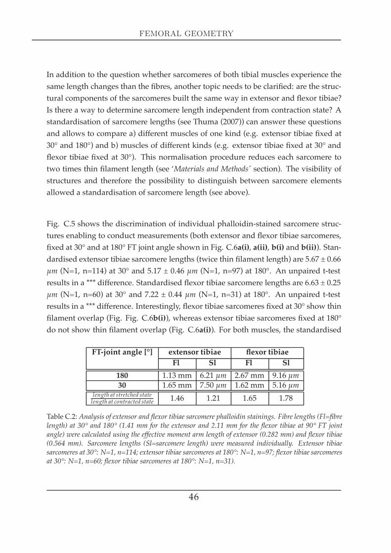
FEMORAL GEOMETRY

In addition to the question whether sarcomeres of both tibial muscles experience thesame length changes than the fibres, another topic needs to be clarified: are the struc-tural components of the sarcomeres built the same way in extensor and flexor tibiae?Is there a way to determine sarcomere length independent from contraction state? Astandardisation of sarcomere lengths (see Thuma (2007)) can answer these questionsand allows to compare a) different muscles of one kind (e.g. extensor tibiae fixed at30° and 180°) and b) muscles of different kinds (e.g. extensor tibiae fixed at 30° andflexor tibiae fixed at 30°). This normalisation procedure reduces each sarcomere totwo times thin filament length (see ‘Materials and Methods´ section). The visibility ofstructures and therefore the possibility to distinguish between sarcomere elementsallowed a standardisation of sarcomere length (see above).

Fig. C.5 shows the discrimination of individual phalloidin-stained sarcomere struc-tures enabling to conduct measurements (both extensor and flexor tibiae sarcomeres,fixed at 30° and at 180° FT joint angle shown in Fig. C.6a(i), a(ii), b(i) and b(ii)). Stan-dardised extensor tibiae sarcomere lengths (twice thin filament length) are 5.67 ± 0.66µm (N=1, n=114) at 30° and 5.17 ± 0.46 µm (N=1, n=97) at 180°. An unpaired t-testresults in a *** difference. Standardised flexor tibiae sarcomere lengths are 6.63 ± 0.25µm (N=1, n=60) at 30° and 7.22 ± 0.44 µm (N=1, n=31) at 180°. An unpaired t-testresults in a *** difference. Interestingly, flexor tibiae sarcomeres fixed at 30° show thinfilament overlap (Fig. Fig. C.6b(i)), whereas extensor tibiae sarcomeres fixed at 180°do not show thin filament overlap (Fig. C.6a(i)). For both muscles, the standardised

FT-joint angle [°] extensor tibiae flexor tibiaeFl Sl Fl Sl

180 1.13 mm 6.21 µm 2.67 mm 9.16 µm30 1.65 mm 7.50 µm 1.62 mm 5.16 µm

length at stretched statelength at contracted state 1.46 1.21 1.65 1.78

Table C.2: Analysis of extensor and flexor tibiae sarcomere phalloidin stainings. Fibre lengths (Fl=fibrelength) at 30° and 180° (1.41 mm for the extensor and 2.11 mm for the flexor tibiae at 90° FT jointangle) were calculated using the effective moment arm length of extensor (0.282 mm) and flexor tibiae(0.564 mm). Sarcomere lengths (Sl=sarcomere length) were measured individually. Extensor tibiaesarcomeres at 30°: N=1, n=114; extensor tibiae sarcomeres at 180°: N=1, n=97; flexor tibiae sarcomeresat 30°: N=1, n=60; flexor tibiae sarcomeres at 180°: N=1, n=31).

46

RESULTS

Figure C.6: LSM sarcomere length measurements on extensor (a(i) and a(ii)) and flexor tibiae muscles(b(i) and b(ii)). The fibres were fixed in situ at either 30° or 180° FT joint angle. Standardisedsarcomere length could be calculated as described in Thuma (2007).

length value is smaller when calculated from the more contracted state compared tothe calculation from the more stretched state. Because even at rest there is some thin-to-thick filament interaction, these increases in thin filament length as muscle fibrelength increases suggest that the thin filaments may have substantial elasticity. Thetotal of standardised extensor tibiae sarcomere lengths was tested to be highly signifi-cantly different (***) from the total of standardised flexor tibiae sarcomere lengths, seeFig. C.7. Mean standardised extensor tibiae sarcomere length is 5.42 µm, mean flexor

47

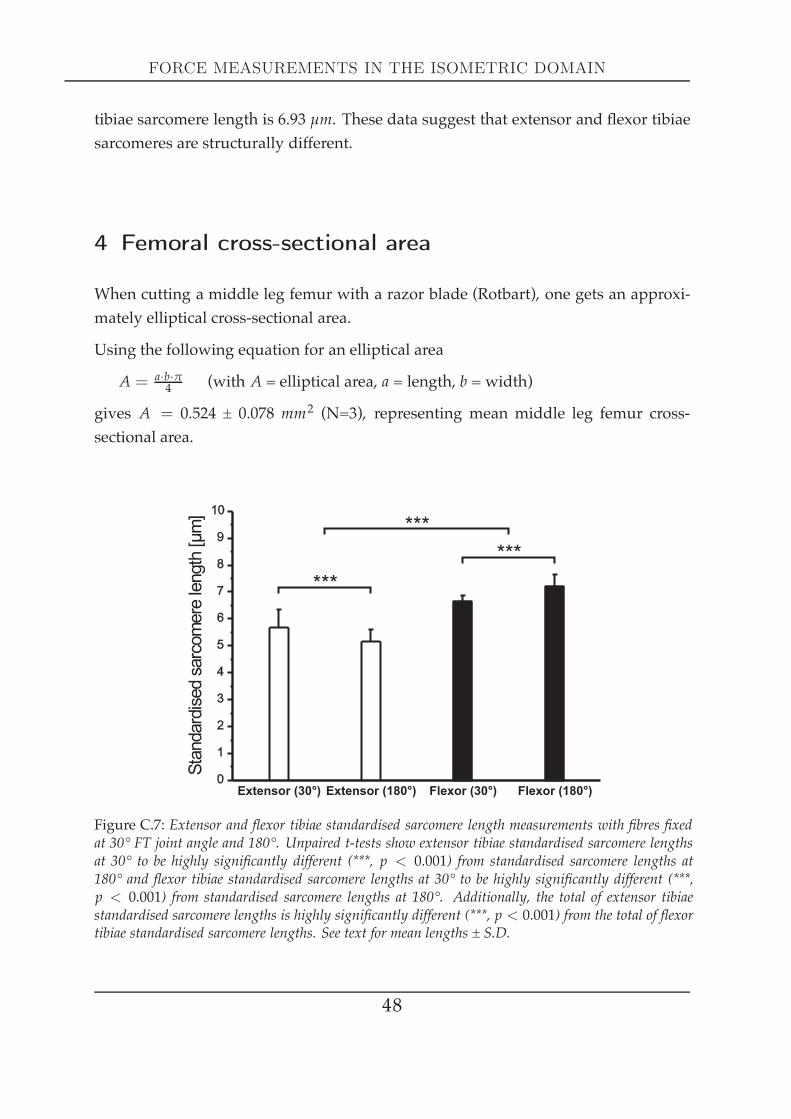
FORCE MEASUREMENTS IN THE ISOMETRIC DOMAIN

tibiae sarcomere length is 6.93 µm. These data suggest that extensor and flexor tibiaesarcomeres are structurally different.

4 Femoral cross-sectional area

When cutting a middle leg femur with a razor blade (Rotbart), one gets an approxi-mately elliptical cross-sectional area.

Using the following equation for an elliptical area

A = a·b·π4 (with A = elliptical area, a = length, b = width)

gives A = 0.524 ± 0.078 mm2 (N=3), representing mean middle leg femur cross-sectional area.

Figure C.7: Extensor and flexor tibiae standardised sarcomere length measurements with fibres fixedat 30° FT joint angle and 180°. Unpaired t-tests show extensor tibiae standardised sarcomere lengthsat 30° to be highly significantly different (***, p < 0.001) from standardised sarcomere lengths at180° and flexor tibiae standardised sarcomere lengths at 30° to be highly significantly different (***,p < 0.001) from standardised sarcomere lengths at 180°. Additionally, the total of extensor tibiaestandardised sarcomere lengths is highly significantly different (***, p < 0.001) from the total of flexortibiae standardised sarcomere lengths. See text for mean lengths ± S.D.

48

RESULTS

C2 Force measurements in theisometric domain

1 Actively generated forces

Extensor tibiae motoneurons were stimulated with single pulses (Fig. C.8) and ton-ically at frequencies ranging from 30 Hz to 200 Hz (see Fig. C.11). The maximumfrequency of 200 Hz was chosen because this is in the range of maximum frequencythat FETi generates during the swing phase of stepping movements (Hooper et al.(2007a); Guschlbauer et al. (2007), 150 Hz in Blaberus discoidalis (Ahn et al. (2006)).Flexor tibiae motoneurons were mainly stimulated with single pulses (Fig. C.9). Ho-mogeneous stimulation of a particular set of motoneurons was possible in only a fewcases using high frequencies without visible stimulation failures in the force trace(C.12). The dual-mode lever system was used exclusively as a force transducer in thischapter.

1.1 Single twitch kinetics

Twitch kinetic measurements included the time to peak force (Tmax), time to 50% re-laxation (T50o f f ) and time to 90% relaxation (T90o f f ), all calculated relative to the forceonset.

As described in ‘Materials and Methods´, suprathreshold extensor tibiae nerve stim-ulation led to one force amplitude (Fig. C.8), because stimulation current should have

49

FORCE MEASUREMENTS IN THE ISOMETRIC DOMAIN

0.02 s

0.5 mN

Stimulus

Figure C.8: Average time course of an examplary single twitch of the extensor tibiae (N=1, n=43).

Table C.3: Extensor tibiae single twitch kinetics.Latency[ms] Pmax [mN] Tmax [ms] T50o f f [ms] T90o f f [ms] N8.5 ± 1.80 2.6 ± 2.45 26.41 ± 6.3 60.69 ± 15.65 149.89± 67.93 12

stimulated mostly all three motoneurons (Bässler and Storrer (1980)). Eventual stimu-lation of only the fast motoneuron could have altered force amplitude only very mod-estly. In contrast, five different flexor tibiae force amplitudes could be determined bycontinous increase of stimulation current amplitude in one animal tested in respect tothis issue (Fig. C.4). Latency of force onset becomes smaller as a consequence of theputative sequential recruitment of more fast motor units. Motoaxons with a smalleraxon diameter need higher current amplitudes to be activated. The conduction ve-locity of an axon is proportional to the square root of the axon diameter (Hodgkinand Huxley (1952); Stein and Pearson (1971); Pearson et al. (1970)). For the extensortibiae, the rough size proportions of the three motoneurons (see ‘Materials and Meth-ods´) are known from Bässler (1977); Bässler and Storrer (1980). Maximal force (Pmax)is within a similar range than the extensor tibiae twitch Pmax (2.6 ± 2.45 mN) for thefirst three single twitch amplitudes (Tabs. C.3 and C.4, lines 1-3). Further increase ofstimulation current leads to doubling of Pmax (Tab. C.4, line 4). Single twitch kinetics(recruitments 1-4) show flexor tibiae fibres to be nearly 3 times faster reaching Pmax(8-10 ms compared to 26 ms, Tabs. C.3 and C.4) and to be 3-6 times faster relaxing,depending on the recruitment level (24-51 ms compared to 150 ms). The reductionin muscle force to prestimulus levels after twitch took in general about 250 ms forthe extensor tibiae, and 60 ms for the flexor tibiae. Maximal extracellular electricallyachieved flexor tibiae twitch force (Tab. C.4, line 5) must be described separately be-

50

RESULTS

0

5

10

15

20

25

30

35

40A

ctiv

ely

genera

ted

forc

e[m

N]

Act

ively

genera

ted

stre

ss[N

/cm

²]

0.0

0.2

0.4

0.6

0.8

1.0

0.00 0.02 0.04 0.06 0.08 0.10 0.12 0.14 0.16 0.18 0.20 0.22 0.24

Figure C.9: Different flexor tibiae single twitch force amplitudes suggesting sequential motoneuronalrecruitment as stimulation current was continously increased (starting with 0 mA) until single twitchforce was not becoming bigger (no ncr recording). As in Fig. C.8, the arrow marks the stimulationonset.

cause of its exceptionally large amplitude. Pmax is 14 times bigger than extensor tibiaetwitches (N=2, one example shown) but kinetics are rather similar for Tmax and T50o f f(21 ms compared to 26 ms and 50 ms compared to 60 ms). T90o f f is 0.6 times faster (90ms compared to 150 ms) but muscle force takes nearly 200 ms to reach prestimuluslevels, compared to 250 ms in the extensor tibiae. The force trace in Fig. C.9 shows alittle shoulder at about 0.06 ms which is likely to represent the force decay of slowerrelaxing fibres that were co-stimulated.

Table C.4: Flexor single twitch kinetics at different recruitment of motor units in one animal.Latency[ms] Pmax [mN] Tmax [ms] T50o f f [ms] T90o f f [ms]

1 11.6 0.6 8 30 512 8.4 2.6 9 19 293 8.4 4.9 10 17 234 8.2 8 9 16 245 7.8 35.5 21 50 90

51

FORCE MEASUREMENTS IN THE ISOMETRIC DOMAIN

The remarkably high contraction amplitude (N=2) led to further investigations. Con-tinous stimulation with 0.2 Hz shows a steady decrease of Pmax that can be describedwith a power function (y = xa). Continous stimulation with 1 Hz shows a fasterdecrease (Fig. C.10a(i), both force traces are temporally set to zero). Log-log appli-cation of maximal force (ordinate) and time (abscissa) proves the force decays to bepower-function-like because y = xa gives log(y) = a · log(x) and the decays can befit with linear regressions (***, Fig. C.10a(ii)) with a R=0.961 for the fit of the 0.2 Hzstimulation data and R=0.978 for the fit of the 1 Hz data). However, the decays havefairly different slopes (-0.0803 and -0.0730). Lin-lin plotting of maximal force vs. pulsecount (instead of time) on the abscissa was done in order to test whether the persistentforce decrease is a temporal or an event-driven effect (Fig. C.10b(i)). The similarityof the linear regression slopes (-0.0826 compared to -0.0829) shown in Fig. C.10b(ii)suggests that force decreases with each pulse, no matter at which frequency. Thereseems to be no regeneration within the next 4 s.

1.2 Force kinetics at different activation

At 30-50 Hz stimulation frequency, twitch contractions merged into an incompletetetanus in all preparations (N=38; Tab. C.5). The summated "steady-state" force am-plitude of the resulting contractions varied between preparations (see Tab. C.6 andFig. C.24). At 80 Hz and higher stimulation frequencies, tetanus was complete in allpreparations. At higher stimulation frequencies, the force level only increased slightlywith increasing stimulation frequency (Fig. C.11, Tab. C.5) and was maximal with nofurther increase at 200 Hz. Maximum force values from 9 preparations are given inTab. C.6.

Summated steady-state force of the flexor tibiae was exclusively tested upon 200 Hzstimulation (see chapter ‘Force in the isotonic domain´). However, in one case it waspossible to achieve a nearly twofold variation of the isometric contraction amplitudeby variation of the stimulation current amplitude (Fig. C.12). Gradation of stimulusamplitude is difficult because the activation thresholds of the flexor tibiae motoneu-

52

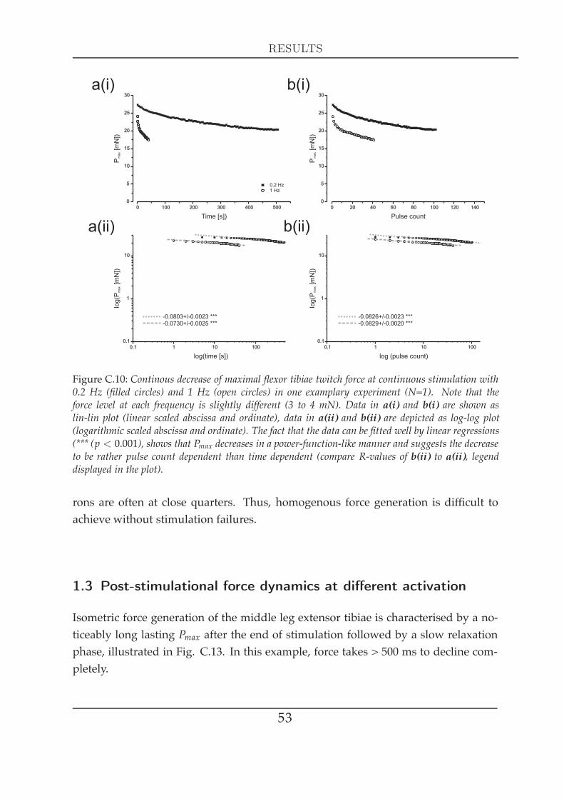
RESULTS

0.1 1 10 1000.1

1

10

log (pulse count)

0.1 1 10 1000.1

1

10

log(time [s])

log(P

[mN

])m

ax

log(P

[mN

])m

ax

P[m

N])

ma

x

P[m

N])

ma

x

0.2 Hz1 Hz

0 100 200 300 400 5000

5

10

15

20

25

30

Time [s])

0 20 40 60 80 100 120 1400

5

10

15

20

25

30

Pulse count

a(i)

a(ii)

b(i)

b(ii)

-0.0803+/-0.0023 *** -0.0826+/-0.0023 ***-0.0730+/-0.0025 *** -0.0829+/-0.0020 ***

Figure C.10: Continous decrease of maximal flexor tibiae twitch force at continuous stimulation with0.2 Hz (filled circles) and 1 Hz (open circles) in one examplary experiment (N=1). Note that theforce level at each frequency is slightly different (3 to 4 mN). Data in a(i) and b(i) are shown aslin-lin plot (linear scaled abscissa and ordinate), data in a(ii) and b(ii) are depicted as log-log plot(logarithmic scaled abscissa and ordinate). The fact that the data can be fitted well by linear regressions(*** (p < 0.001), shows that Pmax decreases in a power-function-like manner and suggests the decreaseto be rather pulse count dependent than time dependent (compare R-values of b(ii) to a(ii), legenddisplayed in the plot).

rons are often at close quarters. Thus, homogenous force generation is difficult toachieve without stimulation failures.

1.3 Post-stimulational force dynamics at different activation

Isometric force generation of the middle leg extensor tibiae is characterised by a no-ticeably long lasting Pmax after the end of stimulation followed by a slow relaxationphase, illustrated in Fig. C.13. In this example, force takes > 500 ms to decline com-pletely.

53

FORCE MEASUREMENTS IN THE ISOMETRIC DOMAIN

30 mN

0.1 s

Force 30 Hz

80 Hz100 Hz200 Hz

50 Hz

Figure C.11: Force development generated upon repetitive stimulation with differing stimulation fre-quencies between 30 Hz and 200 Hz (values in Tab. C.5).

Table C.5: Extensor tibiae tetanus / stress kinetics at different activation levels (N=1 shown examplar-ily).

P0 [mN] / [N · cm−2] T0.5 P0 [ms] T0.9 P0 [ms]30 Hz 84 / 4.39 264 63250 Hz 115 / 6.01 116 24580 Hz 134 / 7.00 85 173100 Hz 140 / 7.31 81 164200 Hz 144 / 7.52 64 132

Considering the fact that most physiologically occuring middle leg swing phases havea duration < 0.2 s (Gabriel et al. (2003); Gabriel and Büschges (2007)), the course ofisometric force after the end of stimulation is a relevant task. Hooper and colleagues(Hooper et al. (2007a)) found muscle time constants in isotonic contractions to be dif-ferent during contraction from during relaxation. Their results show a mean relax-ation τ of 0.055 s (N=7) in response to naturally occuring stimulation input and asustained duration of Pmax (they called it ‘delay to rapid relaxation´) of 0.064 ± 0.014s (N=7). I wondered how long it takes for the extensor tibiae to relax after havinggenerated force in the isometric domain at different activation levels (in comparisonto isotonic experiments performed by Hooper et al.). The persistence of Pmax afterstimulation end was examined as well.

54

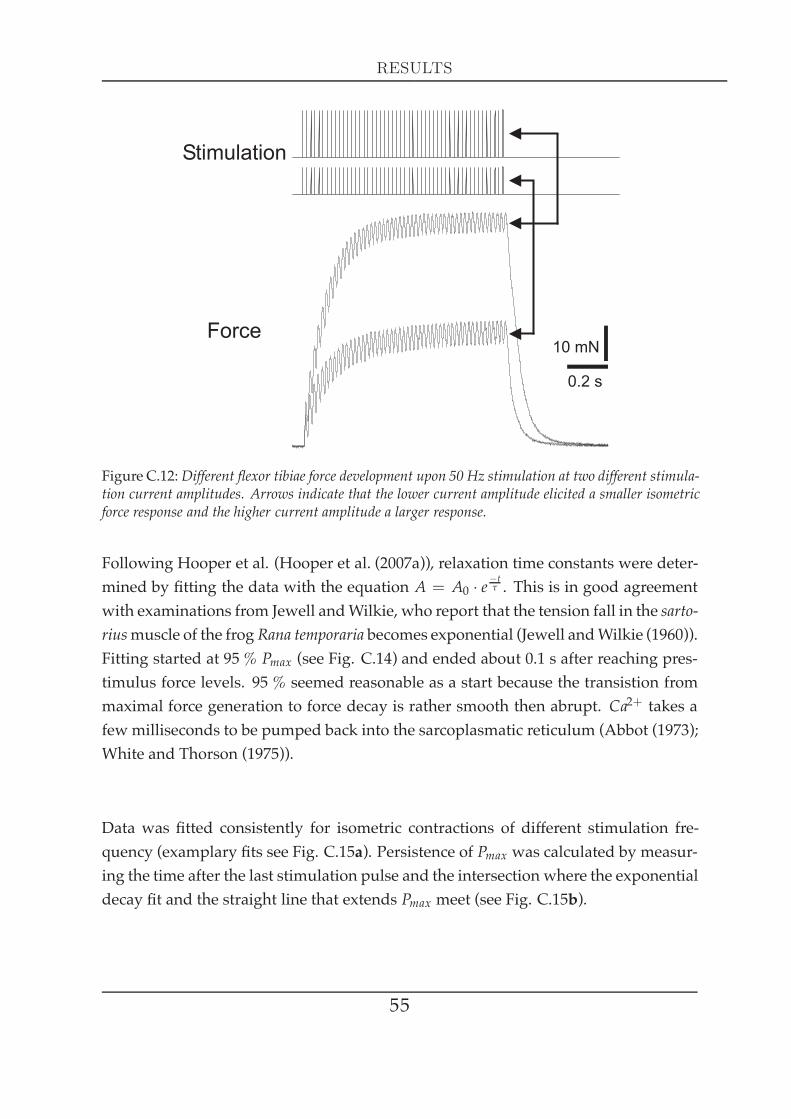
RESULTS

10 mN

0.2 s

Force

Stimulation

Figure C.12:Different flexor tibiae force development upon 50 Hz stimulation at two different stimula-tion current amplitudes. Arrows indicate that the lower current amplitude elicited a smaller isometricforce response and the higher current amplitude a larger response.

Following Hooper et al. (Hooper et al. (2007a)), relaxation time constants were deter-mined by fitting the data with the equation A = A0 · e

−tτ . This is in good agreement

with examinations from Jewell andWilkie, who report that the tension fall in the sarto-riusmuscle of the frog Rana temporaria becomes exponential (Jewell andWilkie (1960)).Fitting started at 95 % Pmax (see Fig. C.14) and ended about 0.1 s after reaching pres-timulus force levels. 95 % seemed reasonable as a start because the transistion frommaximal force generation to force decay is rather smooth then abrupt. Ca2+ takes afew milliseconds to be pumped back into the sarcoplasmatic reticulum (Abbot (1973);White and Thorson (1975)).

Data was fitted consistently for isometric contractions of different stimulation fre-quency (examplary fits see Fig. C.15a). Persistence of Pmax was calculated by measur-ing the time after the last stimulation pulse and the intersection where the exponentialdecay fit and the straight line that extends Pmax meet (see Fig. C.15b).

55

FORCE MEASUREMENTS IN THE ISOMETRIC DOMAIN

30 ms

200 ms

500 ms

20 mN

Figure C.13: Extensor tibiae isometric contraction force takes almost 1 s to reach prestimulus levels.30 ms after the end of stimulation, Pmax has not decreased at all. After 500 ms, Pmax has decreased 50%.

Seven extensor tibiae muscles (N=7) were tested in respect to their relaxation timeconstants, sustained Pmax-durations and Pmax. Data were depicted as absolute values(Fig.C.16a(i), b(i) and c(i) and as relative datapoints normalised to the maximal value(=1.0) in a(ii), b(ii) and c(ii), because of the high degree of variation between ani-mals. In all experiments, relaxation τ and the sustained Pmax-duration increased withincreasing stimulation frequency. Both normalised datapools could be fitted with alinear regression (both ***, R=0.814 for the normalised relaxation τ data and R=0.714for the sustained Pmax - duration data) and increased by 0.2 %

Hz . The relationshipbetween Pmax and stimulation frequency can be described with an exponential satu-ration curve: the higher the activation, the less increase of Pmax.

56

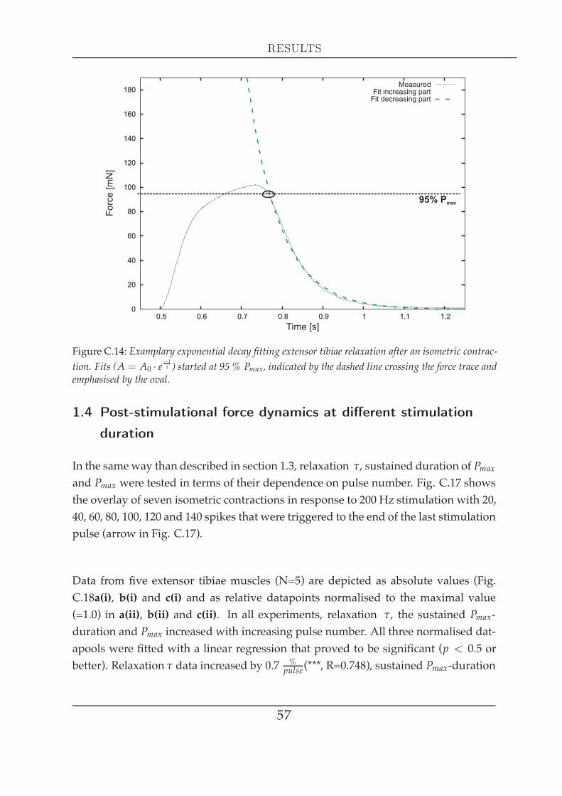
RESULTS

0

20

40

60

80

100

120

140

160

180

0.5 0.6 0.7 0.8 0.9 1 1.1 1.2

Fo

rce

[mN

]

Time [s]

MeasuredFit increasing part

Fit decreasing part

95% Pmax

Figure C.14: Examplary exponential decay fitting extensor tibiae relaxation after an isometric contrac-tion. Fits (A = A0 · e

−tτ ) started at 95 % Pmax, indicated by the dashed line crossing the force trace and

emphasised by the oval.

1.4 Post-stimulational force dynamics at different stimulationduration

In the sameway than described in section 1.3, relaxation τ, sustained duration of Pmaxand Pmax were tested in terms of their dependence on pulse number. Fig. C.17 showsthe overlay of seven isometric contractions in response to 200 Hz stimulation with 20,40, 60, 80, 100, 120 and 140 spikes that were triggered to the end of the last stimulationpulse (arrow in Fig. C.17).

Data from five extensor tibiae muscles (N=5) are depicted as absolute values (Fig.C.18a(i), b(i) and c(i) and as relative datapoints normalised to the maximal value(=1.0) in a(ii), b(ii) and c(ii). In all experiments, relaxation τ, the sustained Pmax-duration and Pmax increased with increasing pulse number. All three normalised dat-apools were fitted with a linear regression that proved to be significant (p < 0.5 orbetter). Relaxation τ data increased by 0.7 %

pulse(***, R=0.748), sustained Pmax-duration

57

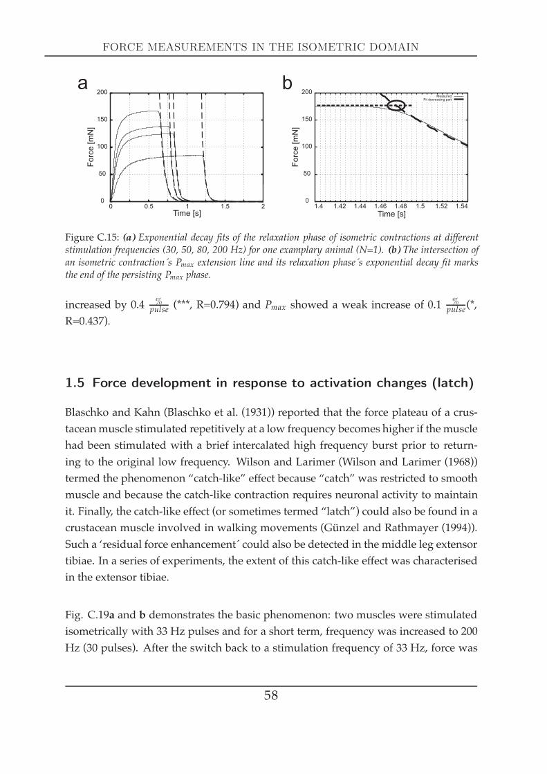
FORCE MEASUREMENTS IN THE ISOMETRIC DOMAIN

0

50

100

150

200

0 0.5 1 1.5Time [s]

Forc

e[m

N]

a

20

50

100

150

200

1.4 1.42 1.44 1.46 1.48 1.5 1.52 1.54

Fo

rce

[mN

]

Time [s]

MeasuredFit decreasing part

b

Figure C.15: (a) Exponential decay fits of the relaxation phase of isometric contractions at differentstimulation frequencies (30, 50, 80, 200 Hz) for one examplary animal (N=1). (b) The intersection ofan isometric contraction´s Pmax extension line and its relaxation phase´s exponential decay fit marksthe end of the persisting Pmax phase.

increased by 0.4 %pulse (***, R=0.794) and Pmax showed a weak increase of 0.1

%pulse(*,

R=0.437).

1.5 Force development in response to activation changes (latch)

Blaschko and Kahn (Blaschko et al. (1931)) reported that the force plateau of a crus-taceanmuscle stimulated repetitively at a low frequency becomes higher if the musclehad been stimulated with a brief intercalated high frequency burst prior to return-ing to the original low frequency. Wilson and Larimer (Wilson and Larimer (1968))termed the phenomenon “catch-like” effect because “catch” was restricted to smoothmuscle and because the catch-like contraction requires neuronal activity to maintainit. Finally, the catch-like effect (or sometimes termed “latch”) could also be found in acrustacean muscle involved in walking movements (Günzel and Rathmayer (1994)).Such a ‘residual force enhancement´ could also be detected in the middle leg extensortibiae. In a series of experiments, the extent of this catch-like effect was characterisedin the extensor tibiae.

Fig. C.19a and b demonstrates the basic phenomenon: two muscles were stimulatedisometrically with 33 Hz pulses and for a short term, frequency was increased to 200Hz (30 pulses). After the switch back to a stimulation frequency of 33 Hz, force was

58

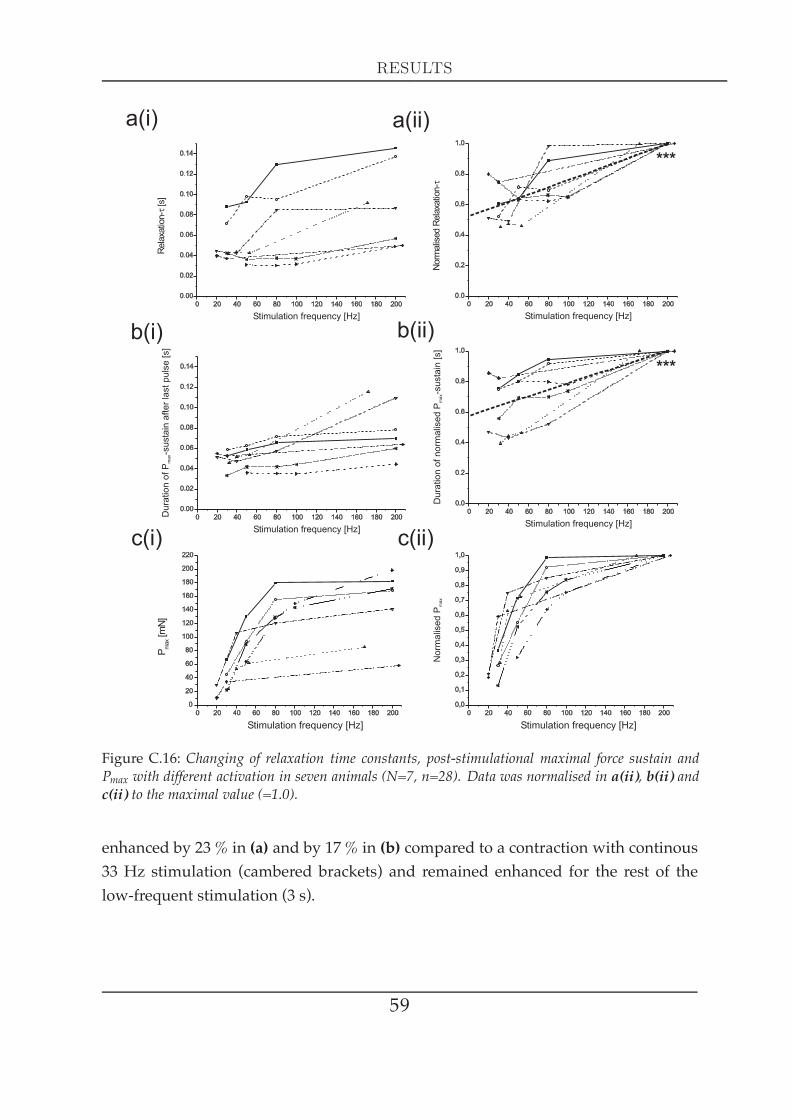
RESULTS

Figure C.16: Changing of relaxation time constants, post-stimulational maximal force sustain andPmax with different activation in seven animals (N=7, n=28). Data was normalised in a(ii), b(ii) andc(ii) to the maximal value (=1.0).

enhanced by 23 % in (a) and by 17 % in (b) compared to a contraction with continous33 Hz stimulation (cambered brackets) and remained enhanced for the rest of thelow-frequent stimulation (3 s).

59

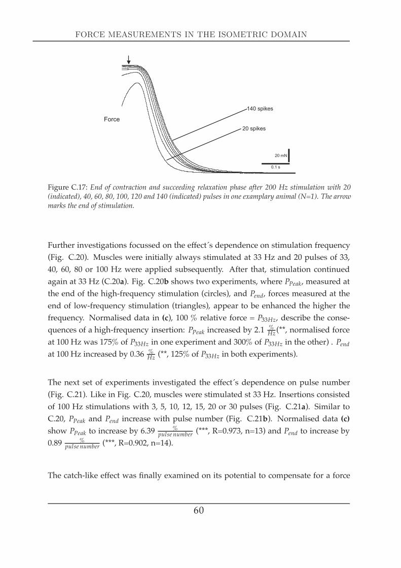
FORCE MEASUREMENTS IN THE ISOMETRIC DOMAIN

20 mN

0.1 s

20 spikes

140 spikes

Force

Figure C.17: End of contraction and succeeding relaxation phase after 200 Hz stimulation with 20(indicated), 40, 60, 80, 100, 120 and 140 (indicated) pulses in one examplary animal (N=1). The arrowmarks the end of stimulation.

Further investigations focussed on the effect´s dependence on stimulation frequency(Fig. C.20). Muscles were initially always stimulated at 33 Hz and 20 pulses of 33,40, 60, 80 or 100 Hz were applied subsequently. After that, stimulation continuedagain at 33 Hz (C.20a). Fig. C.20b shows two experiments, where PPeak, measured atthe end of the high-frequency stimulation (circles), and Pend, forces measured at theend of low-frequency stimulation (triangles), appear to be enhanced the higher thefrequency. Normalised data in (c), 100 % relative force = P33Hz, describe the conse-quences of a high-frequency insertion: PPeak increased by 2.1 %

Hz (**, normalised forceat 100 Hz was 175% of P33Hz in one experiment and 300% of P33Hz in the other) . Pendat 100 Hz increased by 0.36 %

Hz (**, 125% of P33Hz in both experiments).

The next set of experiments investigated the effect´s dependence on pulse number(Fig. C.21). Like in Fig. C.20, muscles were stimulated st 33 Hz. Insertions consistedof 100 Hz stimulations with 3, 5, 10, 12, 15, 20 or 30 pulses (Fig. C.21a). Similar toC.20, PPeak and Pend increase with pulse number (Fig. C.21b). Normalised data (c)show PPeak to increase by 6.39 %

pulse number (***, R=0.973, n=13) and Pend to increase by0.89 %

pulse number (***, R=0.902, n=14).

The catch-like effect was finally examined on its potential to compensate for a force

60

RESULTS

Figure C.18: Changing of relaxation time constants and of post-stimulational maximal force sustainwith different activation duration in seven animals (N=7, n=30). Data was normalised in a(ii), b(ii)and c(ii) to the maximal value (=1.0).

drop during stimulation gaps. The procedure followed the principles of the previousinvestigations shown in Figs. C.20 and C.21: 33 Hz stimulation was interrupted bya brief 20 pulse at 100 Hz stimulation. Additionally, stimulation gaps of various du-ration were included: 0 s, 0.05 s, 0.1s and 0.15 s (Fig. C.22). Data was normalised to

61

FORCE MEASUREMENTS IN THE ISOMETRIC DOMAIN

Figure C.19: a, b: Persisting force increase in response to a short-term 100 Hz burst (N=2). The forceincrease marked by the cambered brackets represents the ‘catch-like effect´, also termed ‘latch´.

P33Hz measured right before high frequency stimulation started (=100 %). Gap dura-tion could be as long as 0.1 s and was still ‘compensated´ by the force enhancementafter the high frequency burst (Fig. C.22b, N=2). Force dropped below P33Hz whenthe stimulation gap exceeded 0.1 s (N=1).

1.6 The force-length relationship at different activation

The isometric force generated by a muscle depends on motoneuron firing rate andmuscle length because of the overlap of the filaments changes asmuscle length changes(Gordon et al. (1966b); Rack andWestbury (1969); Brown et al. (1999); Brown and Loeb(1999)). The dependence of extensor tibiae muscle force upon these parameters wastherefore tested by stimulating the muscle with single stimuli, intermediate (10-80Hz) and high (200 Hz) frequency tonic stimulations.

Fig. C.23 shows (middle leg) extensor tibiae single twitch force, isometric force at 50Hz stimulation frequency and at 200 Hz versus muscle fibre length. Besides the ex-pected general length dependence based on filament overlap (Gordon et al. (1966b)),it becomes apparent that the dependence of force generation on fibre length and stim-ulation frequency varied between experiments. In the single twitch measurements,maximum force varied 8-fold (1.7-13 mN / 0.09-0.68 N

cm2 ), for the 50 Hz stimulation 5-fold (23.4-114.9 mN / 1.22-6.00 N

cm2 ) and for the 200 Hz stimulation 2.7 fold (61.8-165.6mN / 3.23-8.65 N

cm2 ) (see also Tab. C.6).

62

RESULTS

Rela

tive

forc

ein

crease

[%]

0 10 20 30 40 50 60 70 80 90 1000

20

40

60

80

100

120

For

ce[m

N]

Stimulation frequency [Hz]

0 10 20 30 40 50 60 70 80 90 1000

50

100

150

200

250

300

Stimululation frequency [Hz]

25 mN

0.5 s

Stimulation

Force

a

b c

**

**

Figure C.20: (a) Latch in response to short-term stimulation of different frequency (20 pulses of 33,40, 60, 80 and 100 Hz; N=2, n=10). (b), (c) Circles represent forces (PPeak) measured at the end ofhigh-frequency stimulation, triangles represent forces measured at the end of the second part of low-frequency stimulation (Pend). Open symbols denote experiment 1, filled symbols experiment 2. PPeakand Pend are enhanced with increasing frequency (**, R=0.802 for PPeak and **, R=0.898 for Pend). Dataare illustrated relative to non-stop 33 Hz stimulation (= 100% relative force, P33Hz). For details seetext.

Whereas the 200 Hz length dependencies shows maximummuscle force in the upperthird of the working range, the curves with lower stimulation frequencies show atendency of shifted maximum force up to more elongated fibre lengths (Fig. C.23).This shift is known from other muscles (cat, soleusmuscle: Rack andWestbury (1969);cat, caudofemoralismuscle: Brown et al. (1999); Brown and Loeb (1999)).

63

FORCE MEASUREMENTS IN THE ISOMETRIC DOMAIN

25 mN

0.5 s

0 5 10 15 20 25 300

20

40

60

80

100

120

For

ce[m

N]

# spikes

0 5 10 15 20 25 300

50

100

150

200

250

300

# spikes

Re

lativ

efo

rce

incr

ea

se[%

]

Stimulation

Force

a

b c

***

***

Figure C.21: (a) Latch in response to short-term 100 Hz stimulation of different spikenumber (3, 5,10, 12, 15, 20 and 30 pulses; N=2, n=27). (b), (c) Circles represent forces (PPeak) measured at theend of high-frequency stimulation, triangles represent forces measured at the end of the second partof low-frequency stimulation (Pend). Open symbols denote experiment 1, filled symbols experiment 2.PPeak and Pend are enhanced with increasing pulse number (dashed lines indicate linear regressions, ***(p < 0.001), R=0.973 for PPeak and ***, R=0.902 for Pend). Data are illustrated relative to non-stop 33Hz stimulation with an insertion of 3 pulses at 100 Hz (= 100% relative force, P33Hz). For details seetext.

In addition, the extent of this shift could vary between experiments: two exampleswith maximal and minimal frequency dependence of the length at which the muscledevelops maximum force are depicted in Fig. C.24 a, b.

64

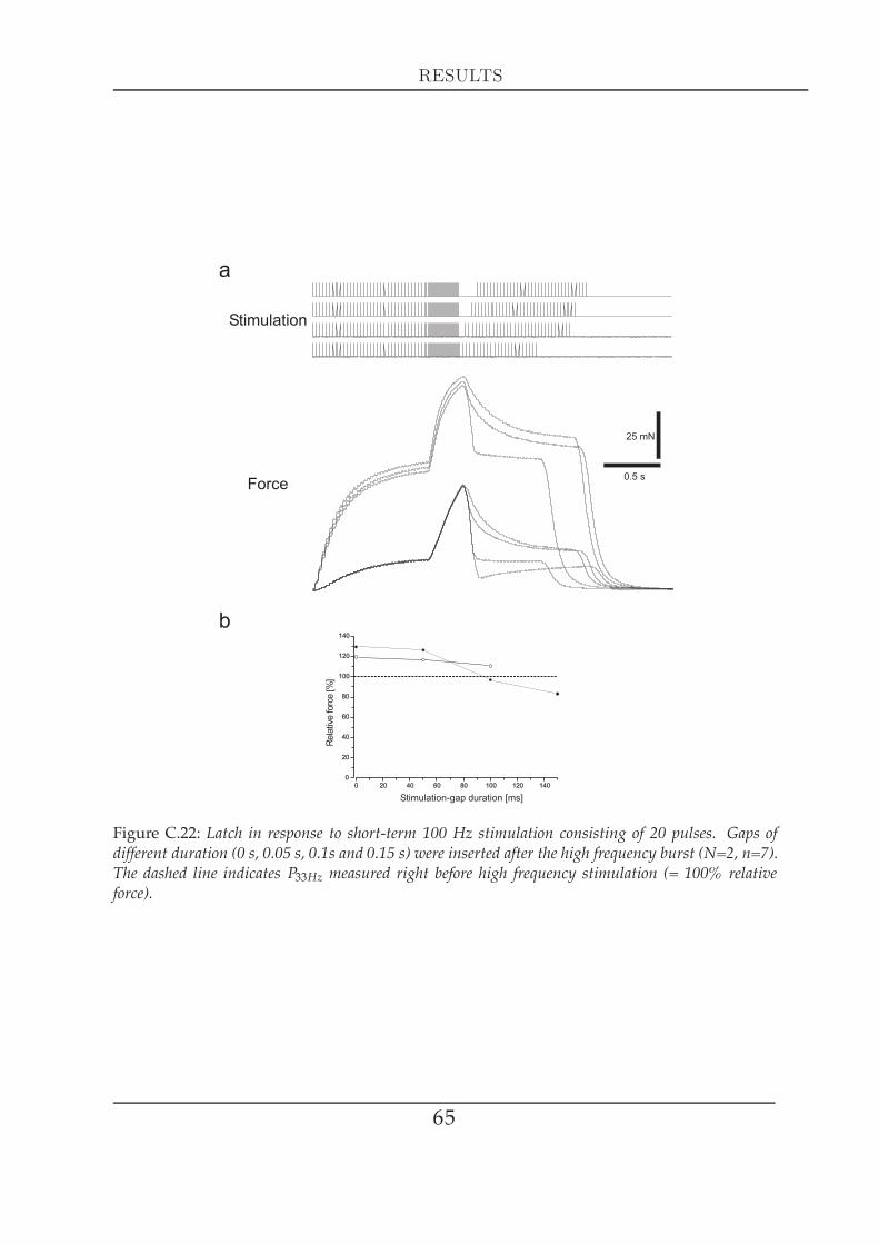
RESULTS

0 20 40 60 80 100 120 1400

20

40

60

80

100

120

140

Rel

ativ

efo

rce

[%]

Stimulation-gap duration [ms]

a

b

25 mN

0.5 s

Stimulation

Force

Figure C.22: Latch in response to short-term 100 Hz stimulation consisting of 20 pulses. Gaps ofdifferent duration (0 s, 0.05 s, 0.1s and 0.15 s) were inserted after the high frequency burst (N=2, n=7).The dashed line indicates P33Hz measured right before high frequency stimulation (= 100% relativeforce).

65

FORCE MEASUREMENTS IN THE ISOMETRIC DOMAIN

Figure C.23: Isometric force (mN, left ordinate) as a function of muscle stretch (mm, lower abscissa)and relative fibre length top abscissa). Values for single twitch (N=8), 50 Hz (N=9) and 200 Hz (N=9),see maximum values in Tab. C.6. For comparison with other muscles, the right ordinate shows stress( Ncm2 ). The working range from 180° (fully stretched joint angle) to 30° (maximal physiologically flexedjoint angle) is marked. Please note that the number for individual means can differ, for single twitchmeasurements 3≤N≤9, for 50 Hz and 200 Hz measurements 5 N≤9.

66

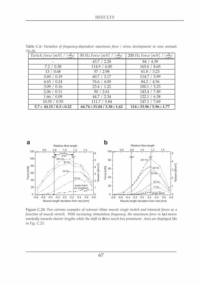
RESULTS

Table C.6: Variation of frequency-dependent maximum force / stress development in nine animals(N=9).Twitch f orce [mN] / [ Ncm2 ] 50 Hz Force [mN] / [ Ncm2 ] 200 Hz Force [mN] / [ Ncm2 ]

- 43.7 / 2.28 84 / 4.397.2 / 0.38 114.9 / 6.00 165.6 / 8.6513 / 0.68 57 / 2.98 61.8 / 3.233.69 / 0.19 60.7 / 3.17 114.7 / 5.994.65 / 0.24 76.6 / 4.00 84.2 / 4.563.09 / 0.16 23.4 / 1.22 100.1 / 5.232.06 / 0.11 50 / 2.61 143.4 / 7.491.66 / 0.09 44.7 / 2.34 122.1 / 6.3810.55 / 0.55 111.7 / 5.84 147.1 / 7.69

5.7± 44.15 / 0.3±0.22 64.74±31.04 / 3.38±1.62 114±33.96 / 5.96±1.77

single twitch(5x amplified)

30 Hz

50 Hz

80 Hz

200 Hz180° 30°

Workingrange

-0.8 -0.6 -0.4 -0.2 0.0 0.2 0.4 0.6 0.80

20

40

60

80

100

120

0

1

2

3

4

5

6

Muscle length deviation from rest [mm]

Forc

e[m

N]

Tensi

on

[N/c

m]

2

aRelative fibre length

0.6 0.8 1.0 1.2 1.4

b

single twitch

207 Hz

60 Hz

30 Hz

20 Hz

17 Hz

-0.8 -0.6 -0.4 -0.2 0.0 0.2 0.4 0.6 0.80

20

40

60

80

Muscle length deviation from rest [mm]

0

1

2

3

4

5100

180° 30°

Tensi

on

[N/c

m]

2

Forc

e[m

N]

Relative fibre length

0.6 0.8 1.0 1.2 1.4

Figure C.24: Two extreme examples of extensor tibiae muscle single twitch and tetanical forces as afunction of muscle stretch. With increasing stimulation frequency, the maximum force in (a) movesmarkedly towards shorter lengths while the shift in (b) is much less prominent. Axes are displayed likein Fig. C.23.

67

PASSIVE FORCES I

C3 Passive forces I

1 Stretch experiments

Stretching an unexcitedmuscle with a step-like displacement stimulus from its restingposition leads immediately to a large force increase followed by a much slower forcedecrease as soon as the displacement stimulus has reached its final position. Theresponse can be separated into a dynamic part with a subsequent decrease becomingby and by an approximate constant static part. Theoretically, following Maxwell´sspring-dashpot model, the stretch of an infinite number of parallel elements leads toan infinitely large force increase. This can be avoided by stretching the muscle withmoderately fast ramps: Fig. C.25 shows the dynamic part with the relaxation onsetexamplified for an extensor tibiae muscle. Within the displayed time frame, the muclehas not yet reached an almost steady-state force value.

1.1 Visco-elastic properties I

The resting tension of a stretched muscle exhibits a phasic-tonic time course due toits visco-elastic properties (Fig. C.25; Bässler and Wegner (1983); Malamud (1989)).In response to a length step stimulus (i.e. an infinitely fast stretch against a velocityproportional friction), the muscle acts instantaneously like a spring. Hookes law F =d · ∆l describes this interrelation: the restoring force of a spring is proportional to thedisplacement of the force application point against the force direction. Due to themuscle being viscous at the same time, the dynamically generated force in responseto such a step stimulus stretch becomes (theoretically) infinitely large because the

68

RESULTS

5 s

0.5 mN0.2 mm

Position

Force

Figure C.25: Passive force development of an unstimulated, denervated middle leg extensor tibiae.Time course of passive force induced by a ramp stretch of 0.5 mm amplitude in 1s. Note the dynamicnature of the force change and its subsequent relaxation at maintained stretch.

mathematical term P = C · t−k→∞ if t = 0 (see Thorson and Biederman-Thorson(1974)). As soon as this instantaneous displacement ends, the muscle starts to flow,like a dashpot whose pistons are moving in oil. In contrast to this viscous muscleproperty, a pure spring would hold the force. Thus, such muscle properties can bedescribed as “visco-” (like a liquid) “-elastic” (like a spring): the muscle is neither areal solid body, nor a real liquid. In contrast to a length step stimulus, the passivemuscle response to a ramp stretch must be described with the term P = C · t1−k, itrepresents the integral of the length step stimulus response. As the displacement isnot instantaneous, the flowing process is happening simultaneously with the stretch.Taking a closer look at such a phasic-tonic time course (Fig. C.26a) reveals two things:

First of all, log-log (double logarithmic) application shows that both increase and de-crease are linear (***, R=0.973 for the increase fit and R=-0.934 for the decrease fit, Fig.C.26b). This means that the course of force development follows a power functioncharacteristic. The muscle response increase follows the equation P = C · t1−k andthe decrease describes again a power function characteristic of the form P = C · t−k

after ∼ 10 times the ramp duration. Thorson and Biedermann-Thorson (Thorson andBiederman-Thorson (1974)) showed that processes with a slowly decaying time con-stant can well described with a power-function characteristic in general. The expo-nent k can be derived from conversion and gives the slope: log(PC ) = −k · log(t). Theconstant C defines the sensitivity in reponse to stretch and describes the stiffness ofthe system. Secondly, the exponents of increase and decrease are different: k = −0.21for the increase and k = 0.16 for the decrease.

69

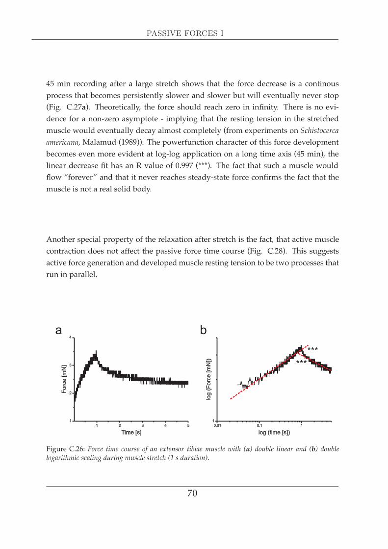
PASSIVE FORCES I

45 min recording after a large stretch shows that the force decrease is a continousprocess that becomes persistently slower and slower but will eventually never stop(Fig. C.27a). Theoretically, the force should reach zero in infinity. There is no evi-dence for a non-zero asymptote - implying that the resting tension in the stretchedmuscle would eventually decay almost completely (from experiments on Schistocercaamericana, Malamud (1989)). The powerfunction character of this force developmentbecomes even more evident at log-log application on a long time axis (45 min), thelinear decrease fit has an R value of 0.997 (***). The fact that such a muscle wouldflow “forever” and that it never reaches steady-state force confirms the fact that themuscle is not a real solid body.

Another special property of the relaxation after stretch is the fact, that active musclecontraction does not affect the passive force time course (Fig. C.28). This suggestsactive force generation and developedmuscle resting tension to be two processes thatrun in parallel.

Figure C.26: Force time course of an extensor tibiae muscle with (a) double linear and (b) doublelogarithmic scaling during muscle stretch (1 s duration).

70

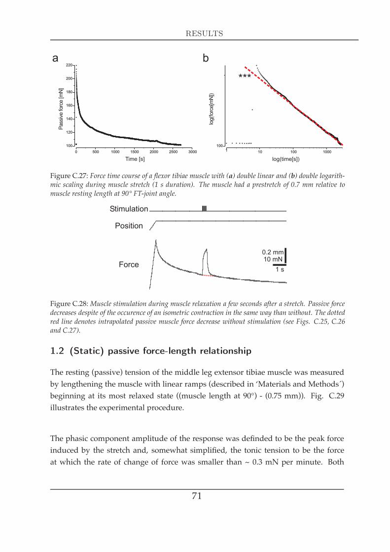
RESULTS

0 500 1000 1500 2000 2500 3000

100

120

140

160

180

200

220P

assi

vefo

rce

[mN

]

Time [s]

a

1 10 100 1000

100

log(

forc

e[m

N])

log(time[s])

b

***

Figure C.27: Force time course of a flexor tibiae muscle with (a) double linear and (b) double logarith-mic scaling during muscle stretch (1 s duration). The muscle had a prestretch of 0.7 mm relative tomuscle resting length at 90° FT-joint angle.

10 mN0.2 mm

1 s

Stimulation

Position

Force

Figure C.28:Muscle stimulation during muscle relaxation a few seconds after a stretch. Passive forcedecreases despite of the occurence of an isometric contraction in the same way than without. The dottedred line denotes intrapolated passive muscle force decrease without stimulation (see Figs. C.25, C.26and C.27).

1.2 (Static) passive force-length relationship

The resting (passive) tension of the middle leg extensor tibiae muscle was measuredby lengthening the muscle with linear ramps (described in ‘Materials and Methods´)beginning at its most relaxed state ((muscle length at 90°) - (0.75 mm)). Fig. C.29illustrates the experimental procedure.

The phasic component amplitude of the response was definded to be the peak forceinduced by the stretch and, somewhat simplified, the tonic tension to be the forceat which the rate of change of force was smaller than ~ 0.3 mN per minute. Both

71

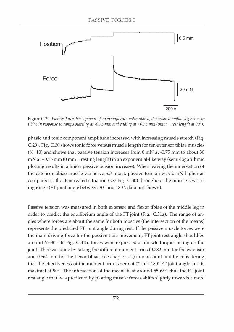
PASSIVE FORCES I

20 mN

0.5 mm

200 s

Position

Force

Figure C.29: Passive force development of an examplary unstimulated, denervated middle leg extensortibiae in response to ramps starting at -0.75 mm and ending at +0.75 mm (0mm = rest length at 90°).

phasic and tonic component amplitude increased with increasing muscle stretch (Fig.C.29). Fig. C.30 shows tonic force versus muscle length for ten extensor tibiae muscles(N=10) and shows that passive tension increases from 0 mN at -0.75 mm to about 30mN at +0.75mm (0mm= resting length) in an exponential-like way (semi-logarithmicplotting results in a linear passive tension increase). When leaving the innervation ofthe extensor tibiae muscle via nerve nl3 intact, passive tension was 2 mN higher ascompared to the denervated situation (see Fig. C.30) throughout the muscle´s work-ing range (FT-joint angle between 30° and 180°, data not shown).

Passive tension was measured in both extensor and flexor tibiae of the middle leg inorder to predict the equilibrium angle of the FT joint (Fig. C.31a). The range of an-gles where forces are about the same for both muscles (the intersection of the means)represents the predicted FT joint angle during rest. If the passive muscle forces werethe main driving force for the passive tibia movement, FT joint rest angle should bearound 65-80°. In Fig. C.31b, forces were expressed as muscle torques acting on thejoint. This was done by taking the different moment arms (0.282 mm for the extensorand 0.564 mm for the flexor tibiae, see chapter C1) into account and by consideringthat the effectiveness of the moment arm is zero at 0° and 180° FT joint angle and ismaximal at 90°. The intersection of the means is at around 55-65°, thus the FT jointrest angle that was predicted by plotting muscle forces shifts slightly towards a more

72

RESULTS

Ten

sio

n[N

/cm

²]

180° 30°Workingrange

Deviation from rest length [mm]-0.8 -0.6 -0.4 -0.2 0.0 0.2 0.4 0.6 0.8

-5

0

5

10

15

20

25

30

35

Relative fibre length

Forc

e[m

N]

0.6 0.8 1.0 1.2 1.4

0.0

0.5

1.0

1.5

Figure C.30: Passive forces of the unstimulated, denervated middle leg extensor tibiae. Tonic restingforce versus muscle length. Data from N=10 experiments (see text for details). Please note that thenumber for individual means can differ (6 ≤ N ≤ 10).

flexed position when doing calculations with the torques acting on the joint.

1.3 Dynamic passive forces

As described above, tibial muscle resting tension appears to be never in a real steadystate. Swing phase duration in a free walking stick insect can become as fast as 0.1 to0.12 s (Cruse (1985a),Büschges and Schmitz (1991); Büschges (1995b)). As the muscleacts like a spring in response to stretch, i.e. fast extension movements like a swingphase for instance, the dynamically achieved passive force e.g. of the flexor tibiaecan become very large. Focussing on the FT joint, the swing phase in the stick in-sect middle leg is mainly determined by activity of the extensor tibiae (Fischer et al.(2001); Schmidt et al. (2001)). The passive force of the flexor tibiae is therefore themain movement opposing force considering the fact that the tibia mass is that lightthat its inertia does not really matter (tibia and tarsus: 3.3 ± 0.2 mg, N=5). Passiveflexor tibiae force amplitude was therefore investigated with ramps simulating swingphase in amplitude and duration (Fig. C.32).

73

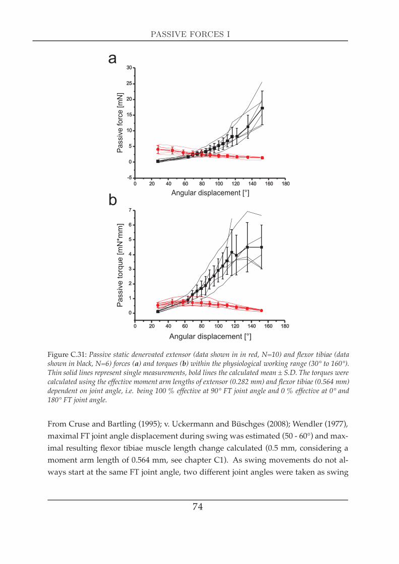
PASSIVE FORCES I

Figure C.31: Passive static denervated extensor (data shown in in red, N=10) and flexor tibiae (datashown in black, N=6) forces (a) and torques (b) within the physiological working range (30° to 160°).Thin solid lines represent single measurements, bold lines the calculated mean ± S.D. The torques werecalculated using the effective moment arm lengths of extensor (0.282 mm) and flexor tibiae (0.564 mm)dependent on joint angle, i.e. being 100 % effective at 90° FT joint angle and 0 % effective at 0° and180° FT joint angle.

From Cruse and Bartling (1995); v. Uckermann and Büschges (2008); Wendler (1977),maximal FT joint angle displacement during swing was estimated (50 - 60°) and max-imal resulting flexor tibiae muscle length change calculated (0.5 mm, considering amoment arm length of 0.564 mm, see chapter C1). As swing movements do not al-ways start at the same FT joint angle, two different joint angles were taken as swing

74

RESULTS

Figure C.32: Passive dynamic force in 13 flexor tibiae muscles in response to a muscle stretch mim-icking swing phase tibia movement in duration and amplitude (0.5 mm in 0.1 s, N=13). Flexor tibiaemuscle stretch started at 90°. Additionally, mean passive force ± S.D. are displayed in red.

start: 90° and 60°. Resulting forces were 68.56 ± 27.92 mNwhen starting at 90° (N=13)and 40.37 ± 14.09 mN when starting at 60° (N=9), see Fig. C.33a. An unpaired t-testshowed that the values were significantly different (*, p < 0.02). In addition, passiveextensor tibiae force was measured in few animals for comparison. Interestingly, re-sulting forces when starting at 90° with the same ramps than applied for the flexortibiae were 64.02 ± 12.22 mN (N=5) and were statistically not different (-, P ≥ 0.05)from flexor tibiae forces starting at the same angle (Fig. C.33b).

Passively generated flexor tibiae force was further investigated with ramps of thesame duration (0.1 s), but different amplitude (Fig. C.34). In two experiments per-formed, passive muscle force increased almost linear in one case and almost expo-nential in the other. More ramp amplitudes in more animals would have to be madein order to draw a clear conclusion.

75

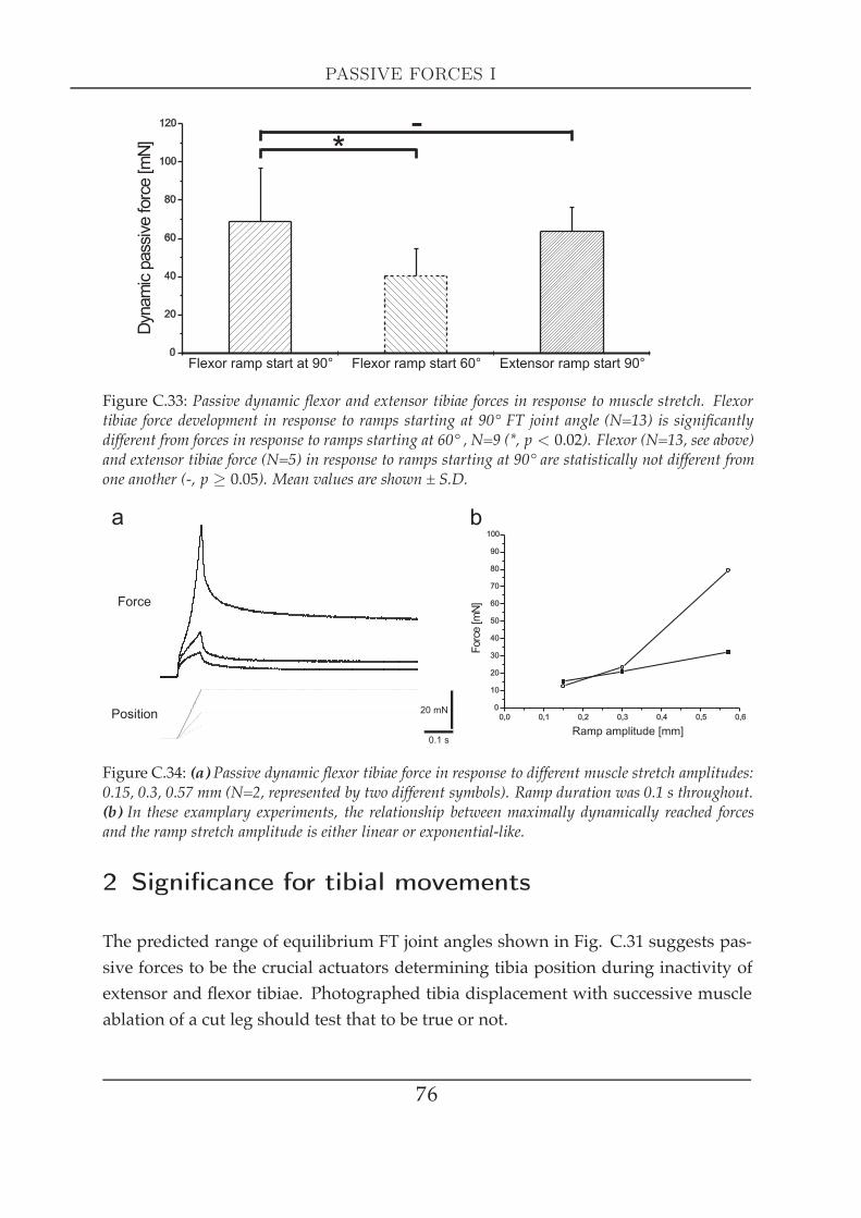
PASSIVE FORCES I

Figure C.33: Passive dynamic flexor and extensor tibiae forces in response to muscle stretch. Flexortibiae force development in response to ramps starting at 90° FT joint angle (N=13) is significantlydifferent from forces in response to ramps starting at 60° , N=9 (*, p < 0.02). Flexor (N=13, see above)and extensor tibiae force (N=5) in response to ramps starting at 90° are statistically not different fromone another (-, p ≥ 0.05). Mean values are shown ± S.D.

0.1 s

20 mN

Force

Position

a

0,0 0,1 0,2 0,3 0,4 0,5 0,60

10

20

30

40

50

60

70

80

90

100

For

ce[m

N]

Ramp amplitude [mm]

b

Figure C.34: (a) Passive dynamic flexor tibiae force in response to different muscle stretch amplitudes:0.15, 0.3, 0.57 mm (N=2, represented by two different symbols). Ramp duration was 0.1 s throughout.(b) In these examplary experiments, the relationship between maximally dynamically reached forcesand the ramp stretch amplitude is either linear or exponential-like.

2 Significance for tibial movements

The predicted range of equilibrium FT joint angles shown in Fig. C.31 suggests pas-sive forces to be the crucial actuators determining tibia position during inactivity ofextensor and flexor tibiae. Photographed tibia displacement with successive muscleablation of a cut leg should test that to be true or not.

76

RESULTS

After either tibia extension or tibia flexion of a cut leg with both muscles intact inone examplary animal (N=1), the tibia returns to nearly 90° with a tendency towardsslight flexion (89 ± 1° after extension, 76 ± 1° after flexion, Fig. C.35a). Ablation ofthe flexor tibiae does solely alter the tibia position after previous extension, only littleafter previous flexion (156 ± 13° after extension, 87 ± 5° after flexion, Fig.C.35b). Afterablation of both muscles, the tibia moved only little from the position where it wasput at (141 ± 7° after extension, 53 ± 5° after flexion, Fig.C.35c). Rotating the joint(so that gravitational force would matter) did not affect the measured angles. Thestatic passive forces shown in Figs. C.30 and C.31 are larger than the 0.03 mN force ofgravity on the mass of tibia and tarsus (3.3 ± 0.2 mg, N=5; see above).

Locusts are known to store large forces in elastic distortions of the tendons and thefemoral cuticle when large forces are generated in femoral muscles, e.g. in prepa-

a b c

Figure C.35:Mean tibia positions ± S.D. in one examplary animal (N=1) with intact muscles (a), theflexor tibiae tendon cut (b), both extensor and flexor tibiae tendon cut (c). The bold line represents thefemur, the thinner line represents the tibia. Arrows mark previous tibial extension (to 180°, n=5 inevery experiment) or flexion (to 30°, n=5 in every experiment).

a b c

Figure C.36: Mean tibia positions ± S.D. in one examplary animal (N=1) with intact joint tissues(a), the outer (extensor tibiae) FT joint tissue ablated (b), both inner (flexor tibiae) and outer (extensortibiae) FT joint tissues ablated (c). Arrows mark previous tibial extension (to 180°, n=5 in everyexperiment) or flexion (to 30°, n=5 in every experiment).

77

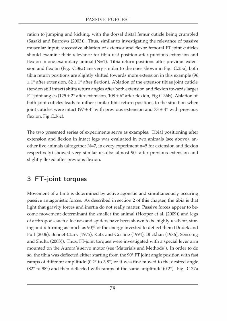
PASSIVE FORCES I

ration to jumping and kicking, with the dorsal distal femur cuticle being crumpled(Sasaki and Burrows (2003)). Thus, similar to investigating the relevance of passivemuscular input, successive ablation of extensor and flexor femoral FT joint cuticlesshould examine their relevance for tibia rest position after previous extension andflexion in one examplary animal (N=1). Tibia return positions after previous exten-sion and flexion (Fig. C.36a) are very similar to the ones shown in Fig. C.35a), bothtibia return positions are slightly shifted towards more extension in this example (96± 1° after extension, 82 ± 1° after flexion). Ablation of the extensor tibiae joint cuticle(tendon still intact) shifts return angles after both extension and flexion towards largerFT joint angles (125 ± 2° after extension, 108 ± 6° after flexion, Fig.C.36b). Ablation ofboth joint cuticles leads to rather similar tibia return positions to the situation whenjoint cuticles were intact (97 ± 4° with previous extension and 73 ± 4° with previousflexion, Fig.C.36c).

The two presented series of experiments serve as examples. Tibial positioning afterextension and flexion in intact legs was evaluated in two animals (see above), an-other five animals (altogether N=7, in every experiment n=5 for extension and flexionrespectively) showed very similar results: almost 90° after previous extension andslightly flexed after previous flexion.

3 FT-joint torques

Movement of a limb is determined by active agonstic and simultaneously occuringpassive antagonistic forces. As described in section 2 of this chapter, the tibia is thatlight that gravity forces and inertia do not really matter. Passive forces appear to be-come movement determinant the smaller the animal (Hooper et al. (2009)) and legsof arthropods such a locusts and spiders have been shown to be highly resilient, stor-ing and returning as much as 90% of the energy invested to deflect them (Dudek andFull (2006); Bennet-Clark (1975); Katz and Gosline (1994); Blickhan (1986); Sensenigand Shultz (2003)). Thus, FT-joint torques were investigated with a special lever armmounted on the Aurora´s servo motor (see ‘Materials and Methods´). In order to doso, the tibia was deflected either starting from the 90° FT joint angle position with fastramps of different amplitude (0.2° to 3.8°) or it was first moved to the desired angle(82° to 98°) and then deflected with ramps of the same amplitude (0.2°). Fig. C.37a

78

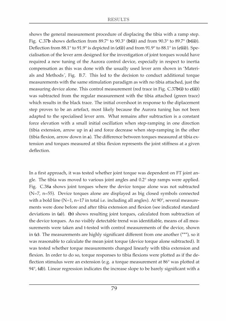
RESULTS

shows the general measurement procedure of displacing the tibia with a ramp step.Fig. C.37b shows deflection from 89.7° to 90.3° (b(i)) and from 90.3° to 89.7° (b(ii)).Deflection from 88.1° to 91.9° is depicted in (c(i)) and from 91.9° to 88.1° in (c(ii)). Spe-cialisation of the lever arm designed for the investigation of joint torques would haverequired a new tuning of the Aurora control device, especially in respect to inertiacompensation as this was done with the usually used lever arm shown in ‘Materi-als and Methods´, Fig. B.7. This led to the decision to conduct additional torquemeasurements with the same stimulation paradigm as with no tibia attached, just themeasuring device alone. This control measurement (red trace in Fig. C.37b(i) to c(ii))was subtracted from the regular measurement with the tibia attached (green trace)which results in the black trace. The initial overshoot in response to the diplacementstep proves to be an artefact, most likely because the Aurora tuning has not beenadapted to the specialised lever arm. What remains after subtraction is a constantforce elevation with a small initial oscillation when step-ramping in one direction(tibia extension, arrow up in a) and force decrease when step-ramping in the other(tibia flexion, arrow down in a). The difference between torques measured at tibia ex-tension and torques measured at tibia flexion represents the joint stiffness at a givendeflection.

In a first approach, it was tested whether joint torque was dependent on FT joint an-gle. The tibia was moved to various joint angles and 0.2° step ramps were applied.Fig. C.38a shows joint torques where the device torque alone was not subtracted(N=7, n=55). Device torques alone are displayed as big closed symbols connectedwith a bold line (N=1, n=17 in total i.e. including all angles). At 90°, several measure-ments were done before and after tibia extension and flexion (see indicated standarddeviations in (a)). (b) shows resulting joint torques, calculated from subtraction ofthe device torques. As no visibly detectable trend was identifiable, means of all mea-surements were taken and t-tested with control measurements of the device, shownin (c). The measurements are highly significant different from one another (***), so itwas reasonable to calculate the mean joint torque (device torque alone subtracted). Itwas tested whether torque measurements changed linearly with tibia extension andflexion. In order to do so, torque responses to tibia flexions were plotted as if the de-flection stimulus were an extension (e.g. a torque measurement at 86° was plotted at94°, (d)). Linear regression indicates the increase slope to be barely significant with a

79

PASSIVE FORCES I

5.00 5.01 5.02 5.03 5.04 5.05-150.4

-75.2

0

75.2

150.4

Time [s]

Tor

que

[mN

*mm

]

0.00 0.01 0.02 0.03 0.04-150.4

-75.2

0

75.2

150.4

Tor

que

[mN

*mm

]

Time [s]

0.00 0.01 0.02 0.03 0.04-150.4

-75.2

0

75.2

150.4

Time [s]

Force insect jointForce measuring deviceForce measuring device + insect joint

Tor

que

[mN

*mm

]

5.00 5.01 5.02 5.03 5.04 5.05-150.2

-75.2

0

75.2

150.4

Time [s]

Tor

que

[mN

*mm

]

b(i) b(ii)

c(ii)c(i)

a

30 mN*mmTorque

Displacement 0.38°

5 s

Figure C.37: Examplary FT-joint torque in response to angular displacement (a), the measuring de-vice´ s lever arm length of 4.75 mm is taken into account. Tibia deflection from 89.7° to 90.3° (b(i)) andfrom 88.1° to 91.9° (c(i)) and back (b(ii) and c(ii)). Displacement trace not shown. Green trace: mea-surement of joint torque including torques arising from the measuring device; red trace: measurementof the device only; black trace: red trace subtracted from green trace, i.e. calculated joint torques.

small R-value (*, 0.04 ≤ p < 0.05, R = 0.32). Thus, within the range of angles tested,joint torques have a weak trend to increase with the tibia being either more extendedor more flexed compared to torque at 90° with a slope of 0.011 mN·mmdeg . In spite of thisweak trend, the mean joint torque was measured (0.068± 0.057mN ·mm). The dataare very scattered, as indicated by the large S.D. and the low R-value (see above).

80

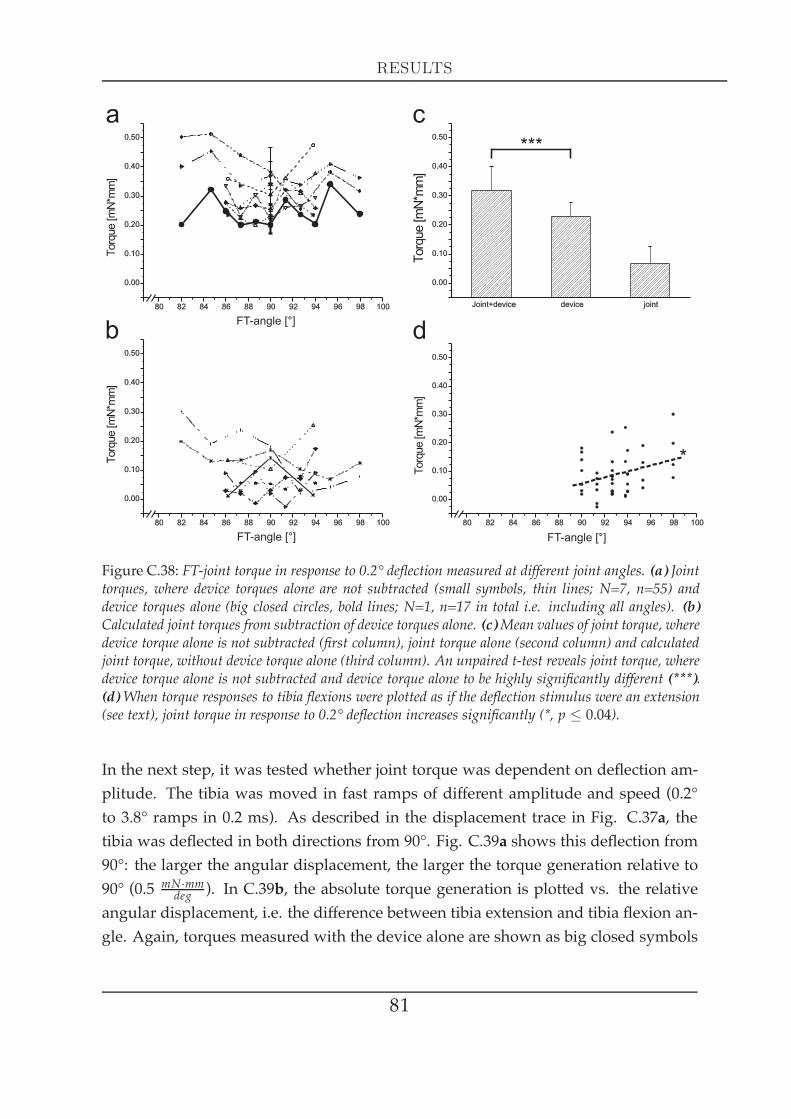
RESULTS

80 82 84 86 88 90 92 94 96 98 100

0.00

0.10

0.20

0.30

0.40

0.50

Tor

que

[mN

*mm

]

FT-angle [°]

80 82 84 86 88 90 92 94 96 98 100

0.00

0.10

0.20

0.30

0.40

0.50

FT-angle [°]

Tor

que

[mN

*mm

]

Joint+device device joint

0.00

0.10

0.20

0.30

0.40

0.50

Tor

que

[mN

*mm

]

80 82 84 86 88 90 92 94 96 98 100

0.00

0.10

0.20

0.30

0.40

0.50

Tor

que

[mN

*mm

]

FT-angle [°]

a c

db

***

*

Figure C.38: FT-joint torque in response to 0.2° deflection measured at different joint angles. (a) Jointtorques, where device torques alone are not subtracted (small symbols, thin lines; N=7, n=55) anddevice torques alone (big closed circles, bold lines; N=1, n=17 in total i.e. including all angles). (b)Calculated joint torques from subtraction of device torques alone. (c)Mean values of joint torque, wheredevice torque alone is not subtracted (first column), joint torque alone (second column) and calculatedjoint torque, without device torque alone (third column). An unpaired t-test reveals joint torque, wheredevice torque alone is not subtracted and device torque alone to be highly significantly different (***).(d)When torque responses to tibia flexions were plotted as if the deflection stimulus were an extension(see text), joint torque in response to 0.2° deflection increases significantly (*, p ≤ 0.04).

In the next step, it was tested whether joint torque was dependent on deflection am-plitude. The tibia was moved in fast ramps of different amplitude and speed (0.2°to 3.8° ramps in 0.2 ms). As described in the displacement trace in Fig. C.37a, thetibia was deflected in both directions from 90°. Fig. C.39a shows this deflection from90°: the larger the angular displacement, the larger the torque generation relative to90° (0.5 mN·mm

deg ). In C.39b, the absolute torque generation is plotted vs. the relativeangular displacement, i.e. the difference between tibia extension and tibia flexion an-gle. Again, torques measured with the device alone are shown as big closed symbols

81

PASSIVE FORCES I

connected with a bold line.

Figure C.39: FT joint torque vs. absolute and relative angular displacement. (a) shows the calculatedtorque generation (with the subtracted device torque) as function of the absolute angular displacement.Linear regression is depicted as bold dashed line (0.5 mN·mm

deg , ***, R = 0.951). (b) shows torquegeneration including measuring device torques (all symbols except for big filled circles; N=5, n=33).Torques measured with the device alone are depicted as big filled circles, connected with a bold line(N=1, n=7).

Figure C.40: Viscoelasticity of the FT joint. Tibial angular displacement causes a joint torque increase(a) / decrease (b) as long as the ramp lasts. Joint torque starts to decrease (a) / increase (b) as soon asthe displacement ends.

To summarise, the FT joint features no clear spring properties because the same dis-placement conducted at different joint angles shows hardly a trend. Nevertheless,

82

RESULTS

there is a dynamic force component because the joint responds with an increase inforce the faster the tibial displacement, it acts like an attenuator (Fig. C.40 a and b).As described above (section 1.1), tibial muscles feature visco-elastic properties and sodoes the FT joint. Interestingly, the net dynamically generated torque development attibia extension (a) is larger than at tibia flexion (b).

83

FORCE MEASUREMENTS IN THE ISOTONIC DOMAIN

C4 Force measurements in theisotonic domain

1 Muscle contractions in response to physiologicalstimulation

Investigation of muscle properties using tonic stimulation input is important to mea-sure characteristics like twitch kinetics or the active force length curve demonstratedin chapter C2, because it is in most cases advantageous to have control upon the inputparameters. However, when measuring muscular output, it is also essential to knowthe mechanisms allowing the animal to transform motoneuronal input into musclecontractions. Hooper et al. (Hooper et al. (2006; 2007a;b)) found several mechanisms,a few are presented here.

As described in ‘Materials and Methods´, contractions from five animals in responseto 87 stimulation regimes of extensor tibiae motoneurons collected from a single legpreparation were investigated. Fig. C.41a shows FETi motoneuron action potentialcount for each performed step-like movement. Mean spike number was 44.2 ± 20.0per step-like movement (a). Distribution of step-like movements vs. spike numberwas Gaussian-like (fit not shown) with the peak at the mean (b). Most steps hadspike numbers ranging from 20 to 60 spikes.

Mean burst duration was 0.41 ± 0.24 s per step-like movement (Fig. C.42a). Very sim-ilar to Fig.C.41, distribution of step-like movements was Gaussian-like with a maxi-

84

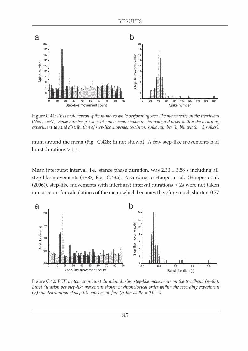
RESULTS

Figure C.41: FETi motoneuron spike numbers while performing step-like movements on the treadband(N=1, n=87). Spike number per step-like movement shown in chronological order within the recordingexperiment (a) and distribution of step-like movements/bin vs. spike number (b, bin width = 3 spikes).

mum around the mean (Fig. C.42b; fit not shown). A few step-like movements hadburst durations > 1 s.

Mean interburst interval, i.e. stance phase duration, was 2.30 ± 3.58 s including allstep-like movements (n=87, Fig. C.43a). According to Hooper et al. (Hooper et al.(2006)), step-like movements with interburst interval durations > 2s were not takeninto account for calculations of the mean which becomes therefore much shorter: 0.77

Figure C.42: FETi motoneuron burst duration during step-like movements on the treadband (n=87).Burst duration per step-like movement shown in chronological order within the recording experiment(a) and distribution of step-like movements/bin (b, bin width = 0.02 s).

85

FORCE MEASUREMENTS IN THE ISOTONIC DOMAIN

± 0.39 s (n=65). This selection was conducted to make sure that only interburst inter-vals within a robust walking sequence of about 1 s (Hooper et al. (2006)) were taken.It was arbitrarily chosen that the animal was very probably quiescent at interburstintervals > 2 s. Distribution is much more scattered than for spike count and burstduration, but has also a very distinct maximum around the mean showing the major-ity of intervals having a duration < 3s (Fig. C.43b).

Fig. C.44 shows contractions of five extensor tibiae muscles in response to two exam-plary, randomly picked stimulation patterns from physiological step-like movements.The individual contractions respond in a similar way and have the same triangularshape. Contraction velocities (the slope of the position signals) and amplitudes areless consistent between animals.

Contraction shape can vary a lot in response to physiological stimulation with pat-terns from locomotory movements. The observed contraction shapes found (Fig.C.45) include: trapezoidal-like shape (a), triangular-like shape (b), multi-slope de-cay (c), (d) and multi-slope increase (e). This figure as well as the following figuresshow data from one animal (N=1, picked randomly) for the sake of phenomenon de-scription, as experiments from five animals (N=5) were consistent.

Figure C.43: FETi motoneuron interburst interval duration during step-like movements on the tread-band (n=87). Interburst interval duration per step-like movement shown in chronological order withinthe recording experiment (a) and distribution of step-like movements/bin (b, bin width = 0.2 s).

86

RESULTS

0.2 mm

0.2 s

N=5

a bStimulation

Position

Figure C.44: Overlay of isotonic contractions of extensors tibiae in response to physiological stimula-tion representing two randomly picked step-like movements (a and b, N=5). Contraction movementdelay arises from muscle force being initially weaker than Aurora lever arm load (min. 3.05 mN, max.15.72 mN).

Visual inspection of physiologically evoked contractions (Figs. C.44 and C.45) sug-gests that the muscle acts like a lowpass filter: contraction shapes look very smootheven though most spike patterns are rather ragged (Hooper et al. (2006; 2007a)). Thisraggedness becomes even clearer when the instananeous frequency of the physiolog-ical stimulation is additionally depicted (Fig. C.46). The three contractions shownare very similar in their contraction amplitude and shape, although their stimulationpatterns look rather different and very ragged in terms of the spikes´ instantaneousfrequency patterns.

Fig. C.47 shows the stimulation (upper trace), the stimulation smoothed with a timeconstant of 0.07 s (like Borgmann et al. (2007)) in the middle trace and the isotonicmuscle contraction in the lower trace, in this case inverted, i.e. muscle shorteningis shown as a positive deflection for better comparison. The apparent similarity be-tween the smoothed stimulation trace and the inverted position in examples (a) to (c)demonstrates the lowpass filter properties of the extensor tibiae: smoothed stimula-tion is reproduced in shape and amplitude in the position trace. Especially Fig. C.47cshows that the relative amplitudes between individual stimulations of the smoothedstimulation trace match the relative position amplitudes.

87

FORCE MEASUREMENTS IN THE ISOTONIC DOMAIN

0.2 mm

0.2 s

a

c d

e

bStimulation

Position

Figure C.45: a-e: Various shapes of contractions in response to physiological stimulation. See text fordetails.

To quantifiy this match, the integral of randomly picked contractions was calculatedand plotted vs. the integral of the smoothed physiological stimulation patterns (Fig.C.48, n=63 from five animals, N=5). Linear regression fitting the data (all fits ***; min-imal R value=0.914, maximal R value=0.992) confirms the visual similarity betweencontraction and smoothed stimulation shown in Fig. (a) to (c). This is in good agree-ment with the analysis of these experiments, which was carried out by Hooper andcolleagues (Hooper et al. (2007a)). They demonstrated that the extensor tibiae actslike a slow filter on the time scale of burst interspike intervals (5-10 ms).

88

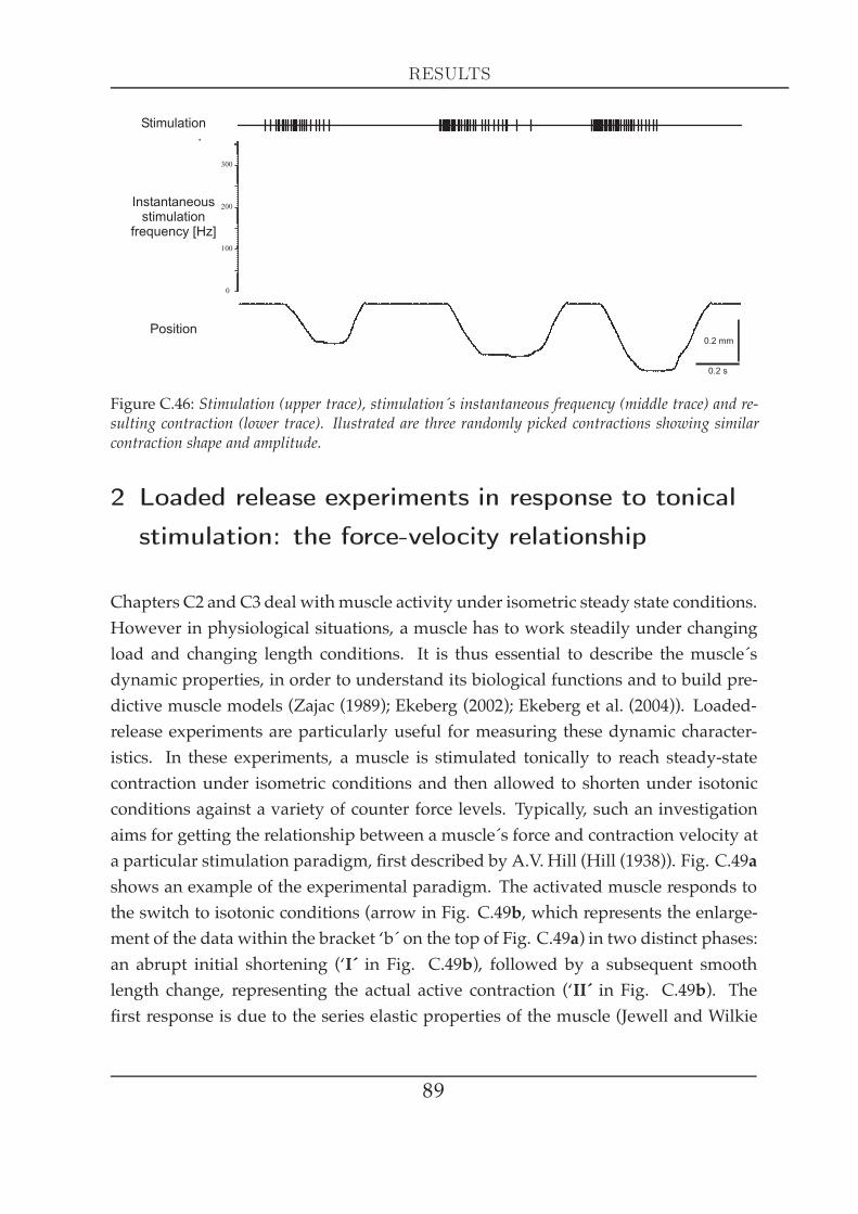
RESULTS

300

200

100

0

0.2 mm

0.2 s

Stimulation

Position

Instantaneousstimulation

frequency [Hz]

Figure C.46: Stimulation (upper trace), stimulation´s instantaneous frequency (middle trace) and re-sulting contraction (lower trace). Ilustrated are three randomly picked contractions showing similarcontraction shape and amplitude.

2 Loaded release experiments in response to tonicalstimulation: the force-velocity relationship

Chapters C2 and C3 deal withmuscle activity under isometric steady state conditions.However in physiological situations, a muscle has to work steadily under changingload and changing length conditions. It is thus essential to describe the muscle´sdynamic properties, in order to understand its biological functions and to build pre-dictive muscle models (Zajac (1989); Ekeberg (2002); Ekeberg et al. (2004)). Loaded-release experiments are particularly useful for measuring these dynamic character-istics. In these experiments, a muscle is stimulated tonically to reach steady-statecontraction under isometric conditions and then allowed to shorten under isotonicconditions against a variety of counter force levels. Typically, such an investigationaims for getting the relationship between a muscle´s force and contraction velocity ata particular stimulation paradigm, first described by A.V. Hill (Hill (1938)). Fig. C.49ashows an example of the experimental paradigm. The activated muscle responds tothe switch to isotonic conditions (arrow in Fig. C.49b, which represents the enlarge-ment of the data within the bracket ‘b´ on the top of Fig. C.49a) in two distinct phases:an abrupt initial shortening (‘I´ in Fig. C.49b), followed by a subsequent smoothlength change, representing the actual active contraction (‘II´ in Fig. C.49b). Thefirst response is due to the series elastic properties of the muscle (Jewell and Wilkie

89

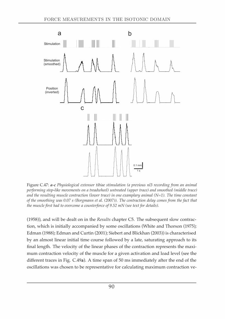
FORCE MEASUREMENTS IN THE ISOTONIC DOMAIN

Position(inverted)

Stimulation(smoothed)

Stimulation

a

c

b

0.1 mm

1 s

Figure C.47: a-c Physiological extensor tibiae stimulation (a previous nl3 recording from an animalperforming step-like movements on a treadwheel) untreated (upper trace) and smoothed (middle trace)and the resulting muscle contraction (lower trace) in one examplary animal (N=1). The time constantof the smoothing was 0.07 s (Borgmann et al. (2007)). The contraction delay comes from the fact thatthe muscle first had to overcome a counterforce of 9.52 mN (see text for details).

(1958)), and will be dealt on in the Results chapter C5. The subsequent slow contrac-tion, which is initially accompanied by some oscillations (White and Thorson (1975);Edman (1988); Edman and Curtin (2001); Siebert and Blickhan (2003)) is characterisedby an almost linear initial time course followed by a late, saturating approach to itsfinal length. The velocity of the linear phases of the contraction represents the maxi-mum contraction velocity of the muscle for a given activation and load level (see thedifferent traces in Fig. C.49a). A time span of 50 ms immediately after the end of theoscillations was chosen to be representative for calculating maximum contraction ve-

90

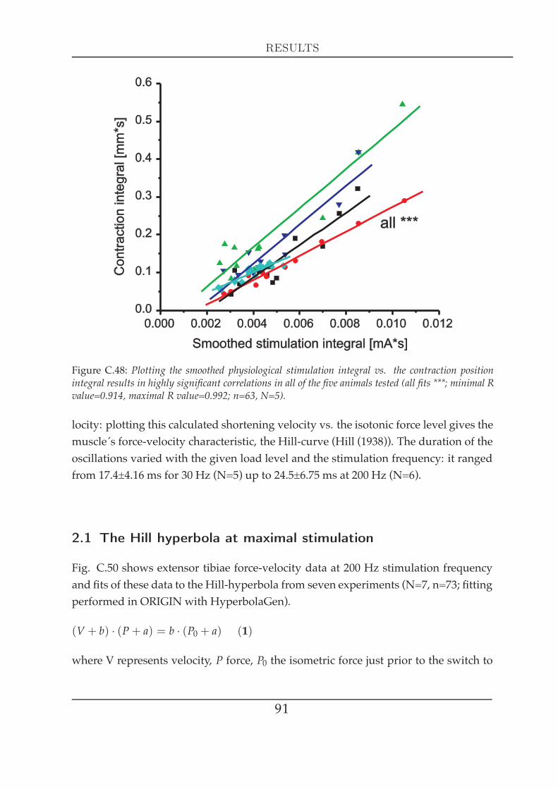
RESULTS

Figure C.48: Plotting the smoothed physiological stimulation integral vs. the contraction positionintegral results in highly significant correlations in all of the five animals tested (all fits ***; minimal Rvalue=0.914, maximal R value=0.992; n=63, N=5).

locity: plotting this calculated shortening velocity vs. the isotonic force level gives themuscle´s force-velocity characteristic, the Hill-curve (Hill (1938)). The duration of theoscillations varied with the given load level and the stimulation frequency: it rangedfrom 17.4±4.16 ms for 30 Hz (N=5) up to 24.5±6.75 ms at 200 Hz (N=6).

2.1 The Hill hyperbola at maximal stimulation

Fig. C.50 shows extensor tibiae force-velocity data at 200 Hz stimulation frequencyand fits of these data to the Hill-hyperbola from seven experiments (N=7, n=73; fittingperformed in ORIGIN with HyperbolaGen).

(V + b) · (P+ a) = b · (P0 + a) (1)

where V represents velocity, P force, P0 the isometric force just prior to the switch to

91

FORCE MEASUREMENTS IN THE ISOTONIC DOMAIN

Figure C.49: The loaded release experiment. (a) Response of a tetanically activated muscle to a switchfrom isometric to isotonic conditions with counter forces less than the force the muscle had developedduring its isometric contraction (different force traces in a). The bracket on top (‘b´) marks the timeframe in which position control switches to force control and the data is shown enlarged in (b): Themuscle shows an abrupt length change (bracket ‘I´) followed by a smooth initially linear contraction(‘II´), see text for details.

isotonic conditions, and “b” and “a” the asymptotes (lying at negative values of P andV).

These data are clearly well fit by a hyperbola (mean R2=0.996 ± 0.006). Different mus-cles show considerable variation in P0 and a smaller variation in V0, the latter beingthe maximum contraction velocity without load. This variability can be removed bynormalising the Hill-equation to P0 and V0 in order to emphasize potential systematicsimilarities:

92

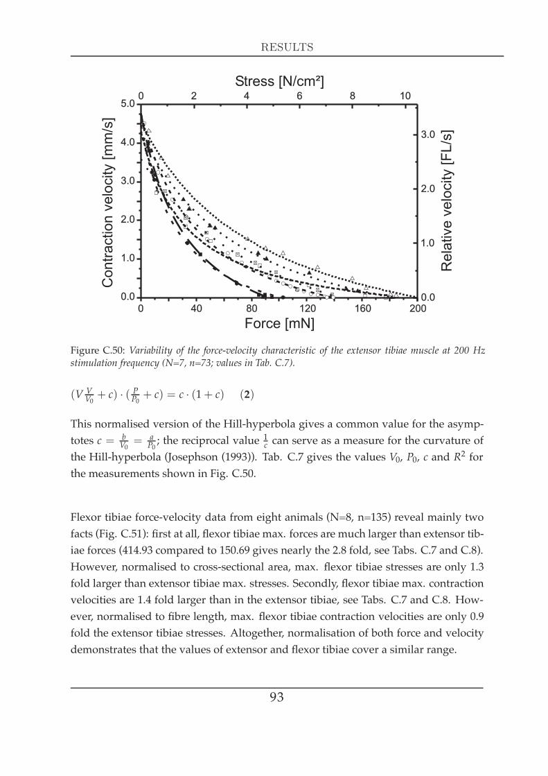
RESULTS

Co

ntr

act

ion

velo

city

[mm

/s]

0

0 2 4 6 8 10

40 80 120 160 2000.0

1.0

2.0

3.0

4.0

5.0

Force [mN]

Stress [N/cm²]

Re

lativ

eve

loci

ty[F

L/s

]

0.0

1.0

3.0

2.0

Figure C.50: Variability of the force-velocity characteristic of the extensor tibiae muscle at 200 Hzstimulation frequency (N=7, n=73; values in Tab. C.7).

(V VV0 + c) · ( PP0 + c) = c · (1+ c) (2)

This normalised version of the Hill-hyperbola gives a common value for the asymp-totes c = b

V0 = aP0 ; the reciprocal value

1c can serve as a measure for the curvature of

the Hill-hyperbola (Josephson (1993)). Tab. C.7 gives the values V0, P0, c and R2 forthe measurements shown in Fig. C.50.

Flexor tibiae force-velocity data from eight animals (N=8, n=135) reveal mainly twofacts (Fig. C.51): first at all, flexor tibiae max. forces are much larger than extensor tib-iae forces (414.93 compared to 150.69 gives nearly the 2.8 fold, see Tabs. C.7 and C.8).However, normalised to cross-sectional area, max. flexor tibiae stresses are only 1.3fold larger than extensor tibiae max. stresses. Secondly, flexor tibiae max. contractionvelocities are 1.4 fold larger than in the extensor tibiae, see Tabs. C.7 and C.8. How-ever, normalised to fibre length, max. flexor tibiae contraction velocities are only 0.9fold the extensor tibiae stresses. Altogether, normalisation of both force and velocitydemonstrates that the values of extensor and flexor tibiae cover a similar range.

93

FORCE MEASUREMENTS IN THE ISOTONIC DOMAIN

Table C.7: Extensor tibiae maximum force / stress, maximum velocity, curvature and R2-value of theHill hyperbola in seven animals (N=7). Values were calculated from the fit (HyperbolaGen, ORIGIN).

P0 [mN] / [ Ncm2 ] V0 [mms ] / [ FLs ] c R2

101.04 / 5.28 4.46 / 3.17 0.28 0.99992.54 / 4.83 4.77 / 3.39 0.36 1138.84 / 7.25 4.75 / 3.38 0.31 0.998194.41 / 10.16 4.28 / 3.04 0.18 0.983183.74 / 9.60 4.31 / 3.07 0.41 0.999201.62 / 10.53 4.56 / 3.24 0.44 0.995142.66 / 7.45 3.59 / 2.55 0.76 0.999

150.69 ± 44.06 / 7.87 ± 2.3 4.39 ± 0.4 / 3.12 ± 0.29 0.39 ± 0.18 0.996 ± 0.006

0

1

2

3

4

5

6

7

8

0 50 100 150 200 250 300 350 400 450 500

Force [mN]

Stress [N/cm²]

Co

ntr

act

ion

velo

city

[mm

/s]

Re

lativ

eve

loci

ty[F

L/s

]

0 2 4 6 8 10 12

0,0

0,5

1,0

1,5

2,0

2,5

3,0

3,5

Figure C.51: Variability of the force-velocity characteristic of the flexor tibiae muscle (N=8, n=135;values in Tab. C.8).

94

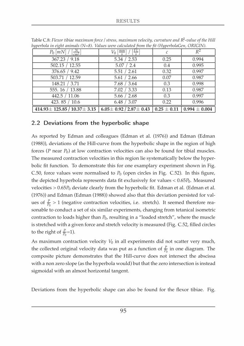
RESULTS

Table C.8: Flexor tibiae maximum force / stress, maximum velocity, curvature and R2-value of the Hillhyperbola in eight animals (N=8). Values were calculated from the fit (HyperbolaGen, ORIGIN).

P0 [mN] / [ Ncm2 ] V0 [mms ] / [ FLs ] c R2

367.23 / 9.18 5.34 / 2.53 0.25 0.994502.15 / 12.55 5.07 / 2.4 0.4 0.995376.65 / 9.42 5.51 / 2.61 0.32 0.997503.71 / 12.59 5.61 / 2.66 0.07 0.987148.21 / 3.71 7.68 / 3.64 0.3 0.998555. 16 / 13.88 7.02 / 3.33 0.13 0.987442.5 / 11.06 5.66 / 2.68 0.3 0.997423. 85 / 10.6 6.48 / 3.07 0.22 0.996

414.93± 125.85 / 10.37± 3.15 6.05± 0.92 / 2.87± 0.43 0.25 ± 0.11 0.994 ± 0.004

2.2 Deviations from the hyperbolic shape

As reported by Edman and colleagues (Edman et al. (1976)) and Edman (Edman(1988)), deviations of the Hill-curve from the hyperbolic shape in the region of highforces (P near P0) at low contraction velocities can also be found for tibial muscles.The measured contraction velocities in this region lie systematically below the hyper-bolic fit function. To demonstrate this for one examplary experiment shown in Fig.C.50, force values were normalised to P0 (open circles in Fig. C.52). In this figure,the depicted hyperbola represents data fit exclusively for values < 0.65P0. Measuredvelocities > 0.65P0 deviate clearly from the hyperbolic fit. Edman et al. (Edman et al.(1976)) and Edman (Edman (1988)) showed also that this deviation persisted for val-ues of P

P0 > 1 (negative contraction velocities, i.e. stretch). It seemed therefore rea-sonable to conduct a set of six similar experiments, changing from tetanical isometriccontraction to loads higher than P0, resulting in a “loaded stretch”, where the muscleis stretched with a given force and stretch velocity is measured (Fig. C.52, filled circlesto the right of PP0 =1).

As maximum contraction velocity V0 in all experiments did not scatter very much,the collected original velocity data was put as a function of PP0 in one diagram. Thecomposite picture demonstrates that the Hill-curve does not intersect the abscissawith a non zero slope (as the hyperbola would) but that the zero intersection is insteadsigmoidal with an almost horizontal tangent.

Deviations from the hyperbolic shape can also be found for the flexor tibiae. Fig.

95

FORCE MEASUREMENTS IN THE ISOTONIC DOMAIN

0.0 0.2 0.4 0.6 0.8 1.0 1.2 1.4 1.6

0.0

1.0

2.0

3.0

4.0

5.0C

ontr

act

ion

velo

city

[mm

/s]

P/P0P/P0

Rela

tive

velo

city

[Fib

rele

ngth

s/s]

0.0

1.0

3.0

2.0

Figure C.52: Deviation of the force-velocity curve (solid line) from hyperbolic shape in the region of PP0between 0.6 and 1 for one typical experiment (open circles). The extensor tibiae muscle was activatedwith a stimulation frequency of 200 Hz. In the region P

P0 > 1 force-velocity measurements are shownunder stretch (filled circles, data from 6 experiments) to demonstrate the sigmoid zero crossing of theHill-hyperbola. The force axis was normalised to the maximum isometric contraction force P0.

C.53 shows an example where this deviation is obvious for values in the region of PP0between 0.6 and 1, when only data < 0.65P0 were fitted. Even though the figure showsonly one experiment, the deviation is very likely to be found in all measurements(N=8), probably not always starting at datapoints > 0.65P0. In the example shown(Fig. C.53), datapoints are visibly shifted towards smaller contraction velocities, aswas also shown for the extensor tibiae in Fig. C.52.

2.3 The Hill hyperbola at different activation levels

Muscle activation is controlled by motoneuron spike frequency. Thus, the influenceof stimulation frequency on the Hill characteristic was systematically investigated.Fig. C.54 shows an example of the Hill-curves obtained from different stimulation

96

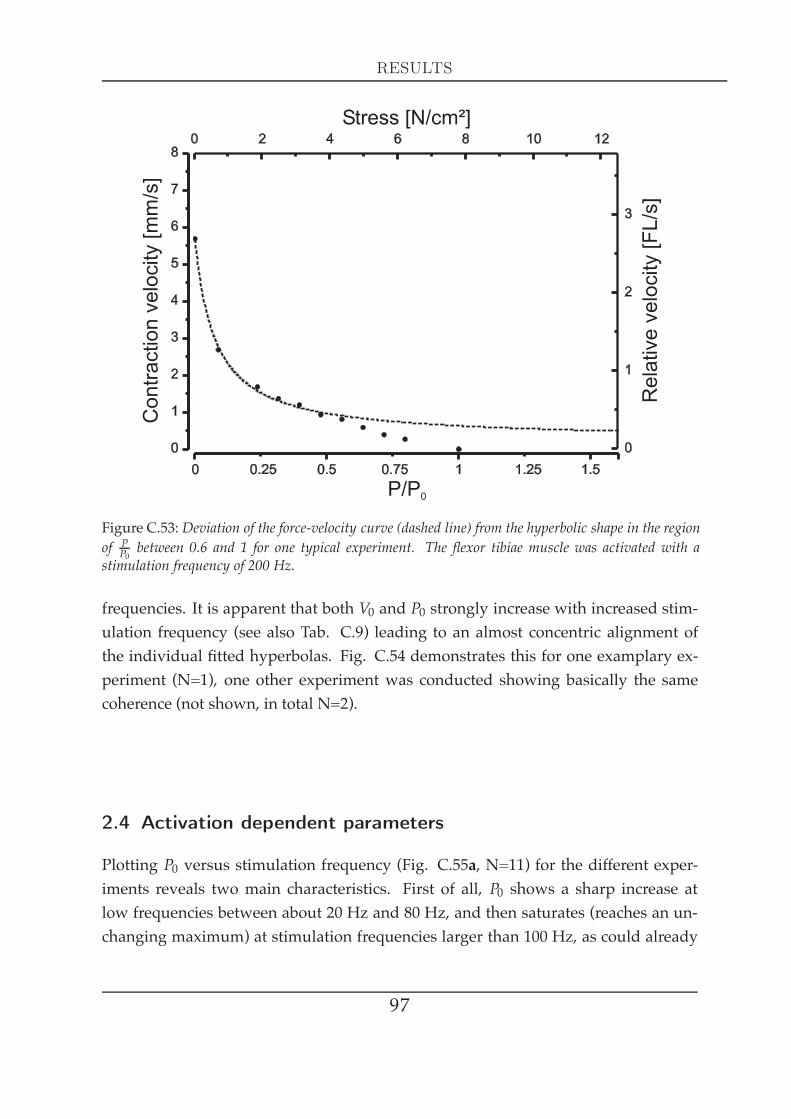
RESULTS

Figure C.53: Deviation of the force-velocity curve (dashed line) from the hyperbolic shape in the regionof P

P0 between 0.6 and 1 for one typical experiment. The flexor tibiae muscle was activated with astimulation frequency of 200 Hz.

frequencies. It is apparent that both V0 and P0 strongly increase with increased stim-ulation frequency (see also Tab. C.9) leading to an almost concentric alignment ofthe individual fitted hyperbolas. Fig. C.54 demonstrates this for one examplary ex-periment (N=1), one other experiment was conducted showing basically the samecoherence (not shown, in total N=2).

2.4 Activation dependent parameters

Plotting P0 versus stimulation frequency (Fig. C.55a, N=11) for the different exper-iments reveals two main characteristics. First of all, P0 shows a sharp increase atlow frequencies between about 20 Hz and 80 Hz, and then saturates (reaches an un-changing maximum) at stimulation frequencies larger than 100 Hz, as could already

97

FORCE MEASUREMENTS IN THE ISOTONIC DOMAIN

0

0 2 4 6 8 10

40 80 120 160 2000.0 0.0

1.0

2.0

3.0

1.0

2.0

3.0

4.0

Force [mN]

Stress [N/cm²]

Ve

loci

ty[m

m/s

]

Re

lativ

eve

loci

ty[m

m/s

]30 Hz50 Hz80 Hz

200 Hz

Figure C.54: Hill curves of the extensor tibiae muscle at different stimulation frequencies from oneanimal (N=1, values in Tab. C.9).

Table C.9: Maximum force / stress, maximum velocity, curvature and R2-value of the Hill hyperbolain the extensor tibiae muscle at different activation in an examplary animal.

P0 [mN] / [N · cm−2] V0 [mm · s−1] / [FL · s−1] c R2

30 Hz 52.82 / 2.76 2.19 / 1.56 0.51 0.99350 Hz 101.1 / 5.28 3.11 / 2.21 0.5 0.99780 Hz 134.97 / 7.05 3.97 / 2.82 0.43 0.997200 Hz 183.74 / 9.60 4.31 / 3.07 0.41 0.999

be observed in Fig. C.16 in chapter C2. Secondly, the maximum saturated force atmaximum stimulation frequency (in this case 200 Hz) varies from about 100 mN upto 190 mN in the different muscles examined. Fitting these data with an exponential

saturation curve P0 = P0max(1− e− ff0 ) in which P0max is the saturation value and f0 is

the frequency at which the curve has reached 1− 1e of its saturation level gave R

2 val-ues of 0.90 ± 0.047 (min. 0.83, max. 0.98) and a mean f 0 of 56.6±17.2 Hz (N=11). Thesteepest and the shallowest fit to the data as well as the mean ± S.D. are added.

Plotting V0 versus frequency can be fitted with a similar function and shows a nearlyidentical dependence with an even higher mean R2 of 0.93 ± 0.06 (min 0.86, max 0.98)

98

RESULTS

and a similar mean f0 of 57.7±17.9 Hz (Fig. C.55b, N=5). Again the steepest and theshallowest fit as well as the mean±S.D. are shown.

The paired data of V0 and P0 in the individual experiments showed in all cases a sig-nificant positive correlation (*, p < 0.03, Fig C.55c, N=5). The ratio V0P0 of the maximumvalues of P0 and V0 at 200 Hz correlate well with the slopes of the regression lines (*,p < 0.05).

Neither a correlation could be found between the frequency constants f0 of the corre-sponding P0 and V0 fits of the individual experiments, nor between the f0 values andthe P0 and V0 values. At present, a similar analysis is not possible for the curvatureparameter ‘c´. This mostly arises from the fact that only a limited number of values for‘c´ were gathered, since the focus was rather to look for pairs of V0 and P0 and not forthe complete Hill-curve in most cases. The available data do not show a systematicchange of ‘c´ with stimulation frequency (not shown). The mean evaluated ‘c´ valuewas 0.5 ± 0.22 (N=14).

2.5 Length dependence of the maximal contraction velocity

Measuring theHill-curves at different muscle lengths and underminimal load demon-strates how maximum contraction velocity V0 depends on muscle length. Two exper-iments were performed to investigate this topic (Fig. C.56). One experiment wasconducted with 200 Hz and with 50 Hz stimulation frequency and with a rest load of0.7 mN compared to a maximum isometric force of 69 (35) mN at 200 (50) Hz (filledsymbols). The other experiment was done solely at 200 Hz (open symbols) at a restload of 4.5 mN compared to the maximum isometric force of 140 mN. Similar to theforce-length characteristics (Fig. C.23,C.24) the velocity-length curves show a mono-tonic and nearly linear increase within the muscle´s working range, followed by aplateau at longer fibre lengths.

99

FORCE MEASUREMENTS IN THE ISOTONIC DOMAIN

Figure C.55: Dependence of the Hill-curve parameters on stimulation frequency in the extensor tibiaemuscle. a Dependence of the isometric force P0 on stimulation frequency (N=11). b Dependence ofmaximum contraction velocity V0 on stimulation frequency (N=5). For both diagrams the data of eachexperiment were fitted by an exponential saturation function leading to the same mean ‘frequency-constant´ f0 of about 60 Hz for both dependencies. In both panels a and b the dotted lines show mostshallow and steepest fits and bold lines show mean ± S.D. Please note that the number for individualmeans can differ (in Fig. a: 6≤N≤9, in Fig. b: 4≤N≤5). c Coupling of maximum contraction velocityV0 with isometric force P0 under variation of stimulation frequencies (N=5). The values of each set ofexperiments are marked by connecting straight lines. For all individual experiments the data showeda significant correlation (p < 0.05). Note that the maximum values V0 and P0 at 200 Hz for eachexperiment determine roughly the overall slopes of the diagrams. See text for details.

3 Isometric and isotonic contraction dynamics atdifferent muscle lengths

Following Gordon et al. (Gordon et al. (1966b)), parts of chapter C2 dealt with therelationship between actively generated force and fibre length (sarcomere length to

100

RESULTS

Figure C.56: Length dependence of maximum contraction velocity V0 in the extensor tibiae (N=2):one experiment was done at 200 Hz and at 50 Hz stimulation frequency (filled symbols). The otherexperiment was done only at 200 Hz (open symbols). See text for details.

be precise). In addition, data in chapter C3 demonstrated that passive static muscleforces increases exponentially with increasing muscle stretch. The following investi-gations went one step further, as not only absolute active force at a particular lengthwas measured, but also the velocity of the force development. This was performed attwo different muscle lengths within the extensor tibiae´s working range. Fig. C.57a(i)shows two data sets: an extensor tibiae muscle was stretched 0.175 mm more thanits length at 90° (red trace) and 0.125 mm less than its length at 90° (black trace) andwas stimulated with a 50 Hz pulse series at both muscle lengths. The measurementsresult in isometric forces (intersections with the ordinate) of 0.18 mN (passive) and94.6 mN (active) in the less stretched state (black trace) and 3.11 mN (passive) and117.97 mN (active) in the more stretched state (red trace). The passive and activeforce increase at the more stretched position compared to the less stretched positionagrees with previously shown data in chapters C2 and C3 and the force-length ex-aminations of Gordon et al. (Gordon et al. (1966b)). In addition, velocity of the forceincrease is presented that was gained by differentiating the force recording in SPIKE2

101

FORCE MEASUREMENTS IN THE ISOTONIC DOMAIN

(time constant of 0.015 s). Force increase accelerates within the first two stimulationpulses to maximum velocity at both muscle length states (stretched and relaxed). At20 mN, velocity becomes continously smaller until it reaches Pmax in both isometriccontractions. Individual pulses are visible because the tetanus is not totally fused at50 Hz. Force increase velocity demonstrates to be 55 % larger in the stretched musclecompared to the muscle being more relaxed (912.5 mN

s , red trace and 588mNs , black

trace).

From experiments conducted in the isotonic domain (muscle shortening was con-ducted against a load being approximately equal to the passive tension at the re-spective length), velocity of the muscle´s displacement is illustrated in Fig. C.57a(ii):exactly like the force increase´s velocity, maximal displacement velocity is reachedwithin the first two stimulation pulses at both contraction states. However, differ-ent from force increase´s velocity, maximal displacement velocity is in the muscle´sstretched state only 7 % larger than in the relaxed one (3.14 mms and 2.94 mm

s ). Afterhaving reached maximum, displacement velocity becomes continously smaller, likethe force velocity depicted in a(i), until it reaches its end position, i.e. the musclelength where the maximal filament overlap is obtained.

The combination of a(i) and a(ii) is illustrated in a figure basically showing three dif-ferent planes: using an algorithm by S. L. Hooper (Hooper et al., in preparation), ve-locities can be depicted as arrows (Fig. C.57b). The length and width of an arrow is ameasure for the velocity amplitude at a given point. Making the assumption that theincrease branches of the force velocity vs. force and the displacement vs. displace-ment velocity plots can be attributed to Ca2+ influx, arrows are exclusively shownstarting at maximal velocity. The figure demonstrates clearly that a muscle at a phys-iologically stretched state generates more active and passive force isometrically (aswould be expected from chapters C2 and C3) and performs to an equal degree morelength change than a relaxed muscle. The ratios of those isometric forces and thoseisotonic displacements (musclestretchedmusclerelaxed ) are very similar: 1.22 for the isometric forces and1.26 for the isotonic displacements.

Force velocity and contraction velocity play a major role when it comes to movementcontrol. Dean (Dean (1984)) found stick insect protractor muscles to maintain suitable

102

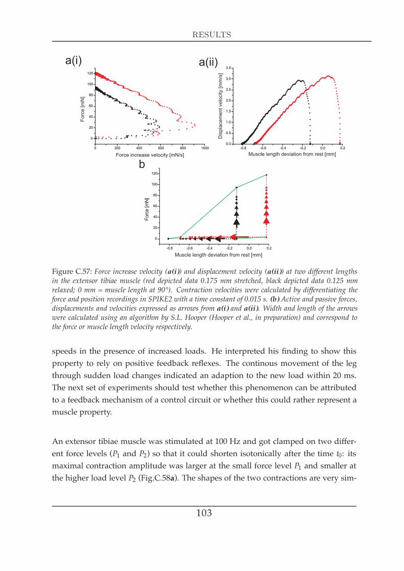
RESULTS

Dis

pla

cem

en

tve

loci

ty[m

m/s

]

Muscle length deviation from rest [mm]

-0.8 -0.6 -0.4 -0.2 0.0 0.20.0

0.5

1.0

1.5

2.0

2.5

3.0

3.5

a(i)

-0.8 -0.6 -0.4 -0.2 0.0 0.2

0

20

40

60

80

100

120

For

ce[m

N]

Muscle length deviation from rest [mm]

x x x x x

xxxx

xxxx

x x x x x x x x

b

Fo

rce

[mN

]

Force increase velocity [mN/s]

0 200 400 600 800 1000

0

20

40

60

80

100

120

a(ii)

Figure C.57: Force increase velocity (a(i)) and displacement velocity (a(ii)) at two different lengthsin the extensor tibiae muscle (red depicted data 0.175 mm stretched, black depicted data 0.125 mmrelaxed; 0 mm = muscle length at 90°). Contraction velocities were calculated by differentiating theforce and position recordings in SPIKE2 with a time constant of 0.015 s. (b) Active and passive forces,displacements and velocities expressed as arrows from a(i) and a(ii). Width and length of the arrowswere calculated using an algorithm by S.L. Hooper (Hooper et al., in preparation) and correspond tothe force or muscle length velocity respectively.

speeds in the presence of increased loads. He interpreted his finding to show thisproperty to rely on positive feedback reflexes. The continous movement of the legthrough sudden load changes indicated an adaption to the new load within 20 ms.The next set of experiments should test whether this phenomenon can be attributedto a feedback mechanism of a control circuit or whether this could rather represent amuscle property.

An extensor tibiae muscle was stimulated at 100 Hz and got clamped on two differ-ent force levels (P1 and P2) so that it could shorten isotonically after the time t0: itsmaximal contraction amplitude was larger at the small force level P1 and smaller atthe higher load level P2 (Fig.C.58a). The shapes of the two contractions are very sim-

103

FORCE MEASUREMENTS IN THE ISOTONIC DOMAIN

ilar: the muscle shortens fast at the beginning, slows down afterwards and saturatesfinally because of maximal degree of thin and thick filament overlap. In a secondapproach (Fig.C.58b), the same muscle is first clamped to P1 and force is switchedto P2 after 0.125 s (t1). The muscle shortens initially as fast as in (a) and continuesshortening, but slower, after the switch to P2. The contraction represents basicallythe combination of the two muscle shortenings depicted in (a). When the muscle isclamped to P1 and is switched to P2 after 0.92 s (t2), the muscle does not continue toshorten: it lengthens immediately and ends at the same contraction amplitude that isreached when switching to P2 earlier (t1 or t0). This contraction represents also thecombination of the two shortenings depicted in (a), with the discrepancy in the timeof the switch: as long as the muscle is in the phase of continous shortening (t1), aswitch to a higher force level will not stop this muscle from shortening. As soon as asaturation of the shortening process is reached, or nearly reached (t2), the muscle willlengthen. This mechanism was verified in four animals (N=4), data from one animalwas taken for illustration.

Figure C.58: Loading at different times during shortening of the extensor tibiae muscle (t0, t1, t2). (a)Isotonic contractions at two different load levels (P1 < P2). (b) Increase of load (P1 → P2) at thebeginning of an isotonic contraction (t1) leads to a continuation of shortening, the same load increaselater in the contraction (t2) leads to a sudden muscle lengthening.

104

RESULTS

C5 Passive forces II

1 Series elasticity

1.1 Series elasticity of tibial muscles at maximal activation

The loaded release experiment shown in Fig. C.49a demonstrated that two thingshappen when a tetanically stimulated muscle is all of a sudden allowed to shorten:first, the muscle in focus experiences a very fast abrupt length change (bracket at ‘I´ inFig. C.49b). Only after that, the muscle shortens actively due to sliding filaments (‘II´in Fig. C.49b). Chapter 3 dealt with this second length change in detail. This sectioninvestigates the first length change.

To analyse the series elasticity (spring constant) of both tibial muscles, the isotonicforce change in the loaded release experiment (steps in the force trace in Fig. C.49a)is plotted versus the associated fast initial length change. Similiar to series elasticitymeasurements in the river toad (depressor mandibulaemuscles in Bufo alvarius, Lappinet al. (2006)), data was calculated by extrapolation of the slope that determines short-ening velocity (see chapter C4): the length difference between this extrapolated slopeand the muscle length before switching to force control at the time of the switch repre-sents the fast shortening of the series elastic component at a given load level (see Fig.C.49b). The SPIKE2 script performing this calculation is added in the Appendix. Inorder to obtain a force-length characteristic comparable with similar measurements inliterature (Wilkie (1956); Jewell and Wilkie (1958)) and with technical spring charac-teristics, the data are presented in the following way: the plot shows the independent,controlled force at the ordinate, the resultant length change on the abscissa for maxi-mal muscle activation, i.e. 200 Hz. The origin length (0 mm) for every set of data was

105

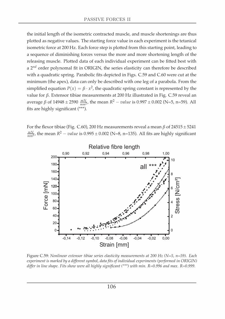
PASSIVE FORCES II

the initial length of the isometric contracted muscle, and muscle shortenings are thusplotted as negative values. The starting force value in each experiment is the tetanicalisometric force at 200 Hz. Each force step is plotted from this starting point, leading toa sequence of diminishing forces versus the more and more shortening length of thereleasing muscle. Plotted data of each individual experiment can be fitted best witha 2nd order polynomal fit in ORIGIN, the series elasticity can therefore be describedwith a quadratic spring. Parabolic fits depicted in Figs. C.59 and C.60 were cut at theminimum (the apex), data can only be described with one leg of a parabola. From thesimplified equation P(x) = β · x2, the quadratic spring constant is represented by thevalue for β. Extensor tibiae measurements at 200 Hz illustrated in Fig. C.59 reveal anaverage β of 14948 ± 2590 mN

mm2 , the mean R2 − value is 0.997 ± 0.002 (N=5, n=59). All

fits are highly significant (***).

For the flexor tibiae (Fig. C.60), 200 Hz measurements reveal a mean β of 24515 ± 5241mNmm2 , the mean R

2 − value is 0.995 ± 0.002 (N=8, n=135). All fits are highly significant

Strain [mm]

Relative fibre length

Fo

rce

[mN

]

Str

ess

[N/c

m²]

-0,14 -0,12 -0,10 -0,08 -0,06 -0,04 -0,02 0,00

0

20

40

60

80

100

120

140

160

180

200

120

0,90 0,92 0,94 0,96 0,98 1,00

0

2

4

6

8

10

all ***

Figure C.59: Nonlinear extensor tibiae series elasticity measurements at 200 Hz (N=5, n=59). Eachexperiment is marked by a different symbol, data fits of individual experiments (performed in ORIGIN)differ in line shape. Fits show were all highly significant (***) with min. R=0.996 and max. R=0.999.

106

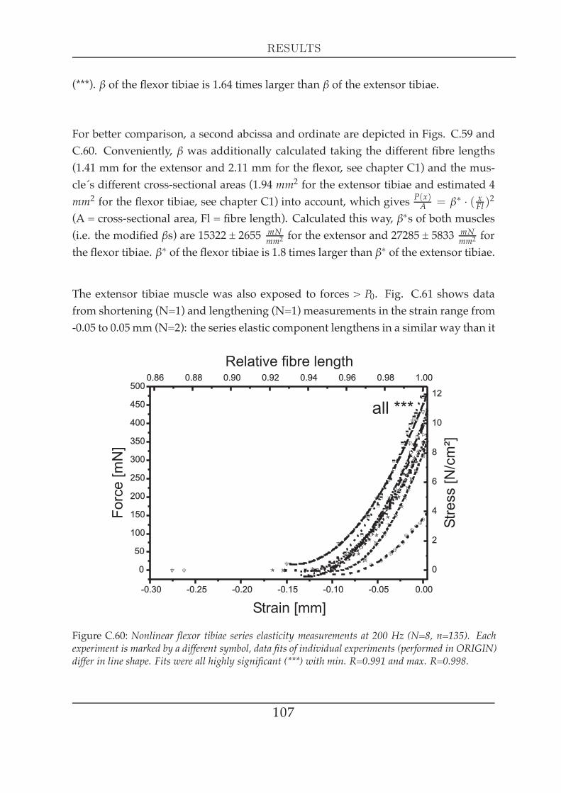
RESULTS

(***). β of the flexor tibiae is 1.64 times larger than β of the extensor tibiae.

For better comparison, a second abcissa and ordinate are depicted in Figs. C.59 andC.60. Conveniently, β was additionally calculated taking the different fibre lengths(1.41 mm for the extensor and 2.11 mm for the flexor, see chapter C1) and the mus-cle´s different cross-sectional areas (1.94 mm2 for the extensor tibiae and estimated 4mm2 for the flexor tibiae, see chapter C1) into account, which gives P(x)

A = β∗ · ( xFl )2

(A = cross-sectional area, Fl = fibre length). Calculated this way, β∗s of both muscles(i.e. the modified βs) are 15322 ± 2655 mN

mm2 for the extensor and 27285 ± 5833mNmm2 for

the flexor tibiae. β∗ of the flexor tibiae is 1.8 times larger than β∗ of the extensor tibiae.

The extensor tibiae muscle was also exposed to forces > P0. Fig. C.61 shows datafrom shortening (N=1) and lengthening (N=1) measurements in the strain range from-0.05 to 0.05mm (N=2): the series elastic component lengthens in a similar way than it

Strain [mm]

Relative fibre length

Fo

rce

[mN

]

Str

ess

[N/c

m²]

-0.30 -0.25 -0.20 -0.15 -0.10 -0.05 0.00

0

50

100

150

200

250

300

350

400

450

5000.86 0.88 0.90 0.92 0.94 0.96 0.98 1.00

0

2

4

6

8

10

12

all ***

Figure C.60: Nonlinear flexor tibiae series elasticity measurements at 200 Hz (N=8, n=135). Eachexperiment is marked by a different symbol, data fits of individual experiments (performed in ORIGIN)differ in line shape. Fits were all highly significant (***) with min. R=0.991 and max. R=0.998.

107

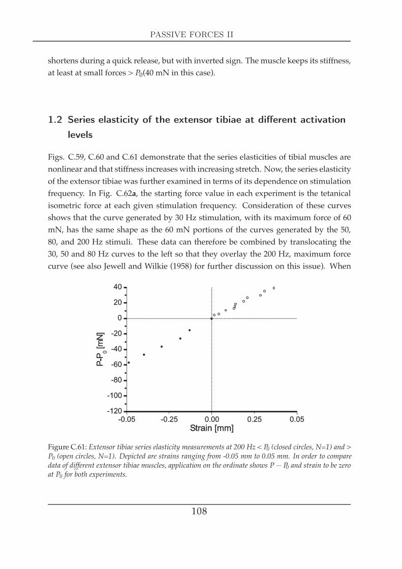
PASSIVE FORCES II

shortens during a quick release, but with inverted sign. The muscle keeps its stiffness,at least at small forces > P0(40 mN in this case).

1.2 Series elasticity of the extensor tibiae at different activationlevels

Figs. C.59, C.60 and C.61 demonstrate that the series elasticities of tibial muscles arenonlinear and that stiffness increases with increasing stretch. Now, the series elasticityof the extensor tibiae was further examined in terms of its dependence on stimulationfrequency. In Fig. C.62a, the starting force value in each experiment is the tetanicalisometric force at each given stimulation frequency. Consideration of these curvesshows that the curve generated by 30 Hz stimulation, with its maximum force of 60mN, has the same shape as the 60 mN portions of the curves generated by the 50,80, and 200 Hz stimuli. These data can therefore be combined by translocating the30, 50 and 80 Hz curves to the left so that they overlay the 200 Hz, maximum forcecurve (see also Jewell and Wilkie (1958) for further discussion on this issue). When

Strain [mm]Strain [mm]

PP

[mN

]-

0

40

20

0

-20

-40

-60

-80

-100

-120-0.05 -0.25 0.25 0.050.00

Figure C.61: Extensor tibiae series elasticity measurements at 200 Hz < P0 (closed circles, N=1) and >P0 (open circles, N=1). Depicted are strains ranging from -0.05 mm to 0.05 mm. In order to comparedata of different extensor tibiae muscles, application on the ordinate shows P− P0 and strain to be zeroat P0 for both experiments.

108

RESULTS

doing so, demonstrated in Fig. C.62b, all force-length curves can be fitted by a singleparabola. In the illustrated experiment (Fig. C.62b), β was 13900 mN

mm2 ; maximumstiffness reached 3150 mN

mm ). It is currently unclear if the spring constant varies withmuscle length, further investigations would be needed to answer this question.

2 Visco-elastic properties II: creep experiments

Chapter 1.6 shows the viscoelastic nature of tibial muscles by ‘deformation with a con-stant rate of strain´, where the strain is increased linearly with time and the stress ismeasured as a function of time. The reverse can be achieved by suddenly applyingstress and maintaining constant while strain is measured as a function of time (afterFerry (1961)). Such experiments are called ‘creep´ experiments are a usual techniquein materials science.

Fig. C.63a illustrates the procedure of such an experiment: a denervated extensortibiae muscle is minimally lengthened by stretch and by simultaneously clampingforce just above the muscle´s resting force level. When the clamped force level sud-denly increases, the muscle responds with a “creeping” strain increase (trace ‘1´ inFig. C.63a). When the muscle is unloaded 10 s later, the muscle does not return to itsoriginal length. The course of this reverse deformation is called ‘creep recovery´. Again10 s later (trace ‘2´ in Fig. C.63a), the muscle is loaded in the same way again andresponds with a length change that is much smaller than before. Again, unloading 10s afterwards does not reestablish the length value before the first loading. Fig. C.63bshows that the measured strains can be well described with a power-function char-acteristic because the data can be fitted with a highly significant linear regression inlog-log application in bothways (all ***, loading R=0.985 and later R=0.999; unloadingR=-0.896 and later R=-0.881).

Fig. C.64 illustrates different forms of creep occuring in different materials:

(a) shows strain to return to its initial value after any time: after t1, when an equlib-rium compliance is not yet reached or after t2, when an equilibrium compliance is ob-tained in the example. Creep and creep recovery can be described with the same func-

109

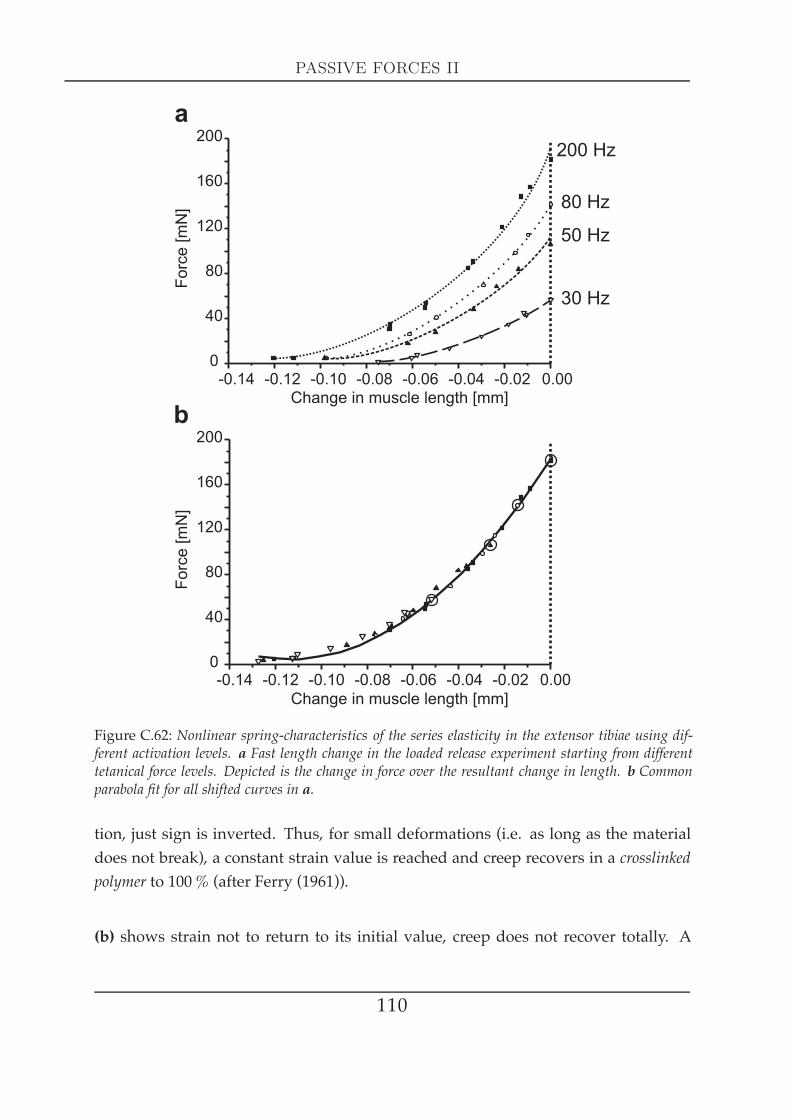
PASSIVE FORCES II

a

b

-0.14 -0.12 -0.10 -0.08 -0.06 -0.04 -0.02 0.00Change in muscle length [mm]

0

40

80

120

160

200

Forc

e[m

N]

-0.14 -0.12 -0.10 -0.08 -0.06 -0.04 -0.02 0.000

40

80

120

160

200

Change in muscle length [mm]

Forc

e[m

N]

30 Hz

50 Hz

80 Hz

200 Hz

Figure C.62: Nonlinear spring-characteristics of the series elasticity in the extensor tibiae using dif-ferent activation levels. a Fast length change in the loaded release experiment starting from differenttetanical force levels. Depicted is the change in force over the resultant change in length. b Commonparabola fit for all shifted curves in a.

tion, just sign is inverted. Thus, for small deformations (i.e. as long as the materialdoes not break), a constant strain value is reached and creep recovers in a crosslinkedpolymer to 100 % (after Ferry (1961)).

(b) shows strain not to return to its initial value, creep does not recover totally. A

110

RESULTS

Figure C.63: Passive extensor tibiae creep. (a) 10 s of stress application and 10 s of release (trace ‘1´),repeated once (trace ‘2´). The second load application leads to a smaller strain increase. (b) Double-logarithmic plotting of the data shows that strain increase (creep) and decrease (creep recovery) can befitted well with linear regressions, i.e. the courses follow a power-function characteristic (all ***).

small deformation leads to a creep approaching a constant value plus a viscous flowcontribution. This viscous flow is responsible that the material does not totally re-cover. This is an example for an uncrosslinked polymer, whose threadlike moleculesare not permanently attached to each other and which has no equilibrium compliance(after Ferry (1961)).

(c) shows creep in the extensor tibiae: here, it looks like an equilibrium compliance

111

PASSIVE FORCES II

is reached (an additional exponential RC-type growth fit is depicted), but creep doesnot totally recover nevertheless. The material nature of the extensor tibiae appears tobe sort of inbetween the materials described in (a) and (b). Its measured propertiescannot be described satisfactorily with a linear power function model.

The above described creep properties raise the question whether it is possible for themuscle to recover from from creep or whether this is an irreversible process, suggest-ing material damage. Fig. C.65 shows creep and incomplete creep recovery. Duringthe recovery a short burst is applied and leads to a large contraction because the loadpulling on the muscle was just slightly larger than the muscle´s resting tension. Af-ter the contraction, the muscle creeps to its initial strain value (and further) againsuggesting that there is no real steady state where passive tension is at steady-state.Finally, creep is reversible and muscle strain can be reset by active thick and thinfilament slide.

The description and comparison of materials with creep experiments was also takenon a more quantitative level. Muscle strain and stress clamp where applied simulta-neously, on one hand resulting in a few milliseconds of oscillations (Fig. C.66a), onthe other hand having the advantage to measure under controlled conditions, becausethe initial muscle length is always the same. The time range used for calculations wasin all quantitative creep examinations 85 ms. A test linear fit with a time range of 850ms (not shown) resulted only in a slight increase of the R value. Taking such a largetime range for analysis had the disadvantage, that muscle strain at large muscle stresslevels could not be analysed because muscle stretch was chosen to be not too large inorder to prevent muscle damage, and therefore 85mswere chosen for determinations.As shown in Fig.C.63b, the strain courses in response to the stress levels depicted inthe upper trace of Fig. C.66a are linear (all fits *** with R values ≥ 0.992), demon-strating that the courses follow powerfunction-characteristics of the form L = C · tk

(in comparison to this force step stimulus, the length step stimulus reponse followsP = C · t−k, see chapter C3). Conversion gives log(L) = log(C) + k · log(t). k is theslope and log(C) the intersection with the ordinate in Fig. C.66b. C represents theamplification and should be changing with increasing stress, which is obvious fromFig. C.66b. k should be independent from stress which can also be reconstructed fromFig. C.66b, as the slopes are apparently parallel to one another.

112

RESULTS

0

0.05

0.1

0.15

0.2

0.25

0 2 4 6 8 10 12 14 16 18 20

Time [s]

Dis

pla

cem

en

t[m

m]

MeasuredFit increasing part

0

0.05

0.1

0.15

0.2

0.25

0 2 4 6 8 10 12 14 16 18 20

MeasuredFit increasing part

a

b

c

Figure C.64: Sheer creep and creep recovery shown schematically for (a) a cross-linked polymer, (b) anuncross-linked polymer, (c) the extensor tibiae. (a) and (b) are adapted after Ferry (1961). The dashedline in (c) denotes an exponential RC-type growth fit.

Creeps were measured of two extensor-flexor tibiae pairs, i.e. one pair from one an-imal respectively (N=2, n=4). In order to compare the material properties of bothmuscles, strains were expressed as the ratio C [mm]

Fibre length [mm] and are therefore nondi-mensional (for fibre lengths, see chapter C1). Stresses were expressed as the ratio

113

PASSIVE FORCES II

20 mN

10 s

0.2 mm

Stimulation

Stress

Strain

Figure C.65: Short high frequency stimulation resets extensor tibiae muscle length after load.

1E-3 0,01 0,1 11E-3

0,01

0,1

1

log(time [s])

log

(po

sitio

n[m

m])

1E-3 0,01 0,1 11E-3

0,01

0,1

1

0.05 mm8 mN

0.01 s

Stress

Position

a b

}***

Figure C.66: Examplary creep experiment. (a) Stress is applied to a passive muscle during simulta-neous muscle stretch (upper trace). The resulting muscle creep is measured (lower trace). The verticaldashed lines indicate the time range used for calculations (in all experiments 85 ms). (b) Double log-arithmic plot showing the power-function characteristics of the creeps depicted in (a) as the differentcreep courses have a linear developing (all linear regression fits ***, p < 0.001).

P [N]Muscle cross−sectional area [cm2] (for cross-sectional areas, see chapter C1). The slope

StrainStress

gives the muscle´s compliance. When plotting so (Fig. C.67a and b), two differentresults arise. For one muscle pair (a), the compliance of extensor and flexor tibiaematch very well: 2.51 cm2

N for the extensor tibiae (***, R=0.998) and 2.08 cm2N for the

114

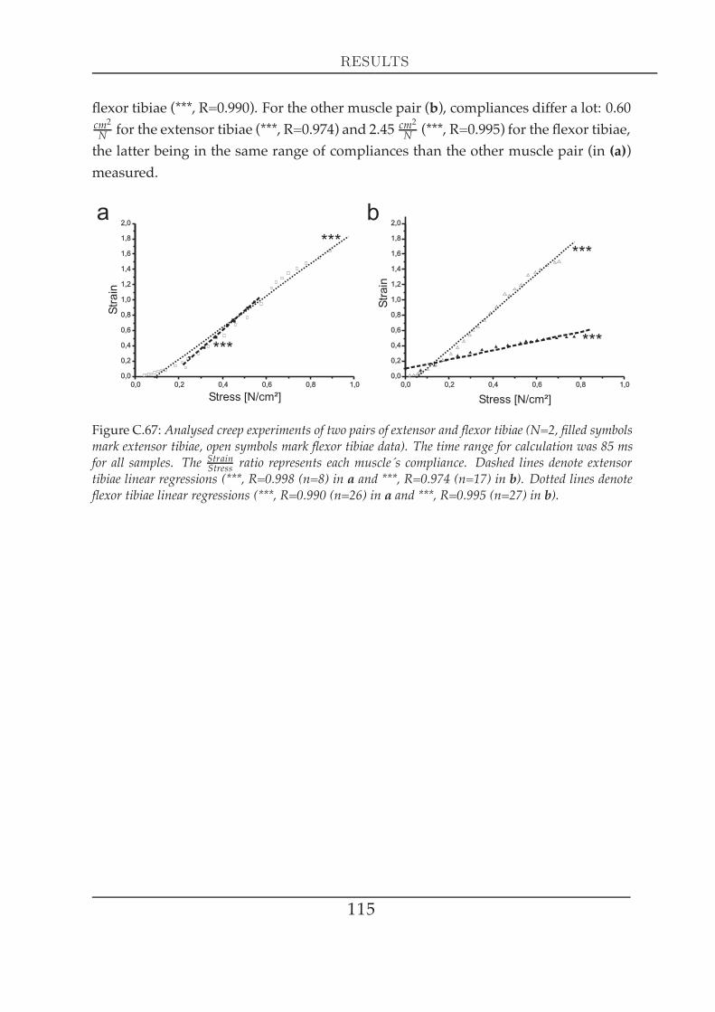
RESULTS

flexor tibiae (***, R=0.990). For the other muscle pair (b), compliances differ a lot: 0.60cm2N for the extensor tibiae (***, R=0.974) and 2.45 cm2N (***, R=0.995) for the flexor tibiae,the latter being in the same range of compliances than the other muscle pair (in (a))measured.

0,0 0,2 0,4 0,6 0,8 1,00,0

0,2

0,4

0,6

0,8

1,0

1,2

1,4

1,6

1,8

2,0

Stress [N/cm²] Stress [N/cm²]

Str

ain

Str

ain

0,0 0,2 0,4 0,6 0,8 1,00,0

0,2

0,4

0,6

0,8

1,0

1,2

1,4

1,6

1,8

2,0a b

***

***

***

***

Figure C.67: Analysed creep experiments of two pairs of extensor and flexor tibiae (N=2, filled symbolsmark extensor tibiae, open symbols mark flexor tibiae data). The time range for calculation was 85 msfor all samples. The StrainStress ratio represents each muscle´s compliance. Dashed lines denote extensortibiae linear regressions (***, R=0.998 (n=8) in a and ***, R=0.974 (n=17) in b). Dotted lines denoteflexor tibiae linear regressions (***, R=0.990 (n=26) in a and ***, R=0.995 (n=27) in b).

115

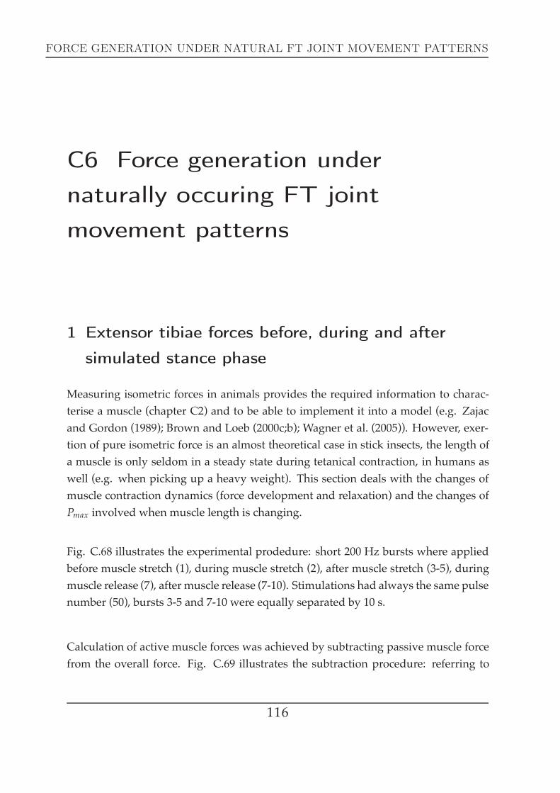
FORCE GENERATION UNDER NATURAL FT JOINT MOVEMENT PATTERNS

C6 Force generation undernaturally occuring FT jointmovement patterns

1 Extensor tibiae forces before, during and aftersimulated stance phase

Measuring isometric forces in animals provides the required information to charac-terise a muscle (chapter C2) and to be able to implement it into a model (e.g. Zajacand Gordon (1989); Brown and Loeb (2000c;b); Wagner et al. (2005)). However, exer-tion of pure isometric force is an almost theoretical case in stick insects, the length ofa muscle is only seldom in a steady state during tetanical contraction, in humans aswell (e.g. when picking up a heavy weight). This section deals with the changes ofmuscle contraction dynamics (force development and relaxation) and the changes ofPmax involved when muscle length is changing.

Fig. C.68 illustrates the experimental prodedure: short 200 Hz bursts where appliedbefore muscle stretch (1), during muscle stretch (2), after muscle stretch (3-5), duringmuscle release (7), after muscle release (7-10). Stimulations had always the same pulsenumber (50), bursts 3-5 and 7-10 were equally separated by 10 s.

Calculation of active muscle forces was achieved by subtracting passive muscle forcefrom the overall force. Fig. C.69 illustrates the subtraction procedure: referring to

116

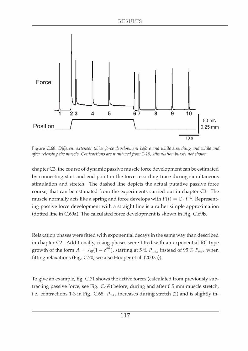
RESULTS

50 mN

0.25 mm

10 s

1 2 3 4 5 6 7 8 9 10

Force

Position

Figure C.68: Different extensor tibiae force development before and while stretching and while andafter releasing the muscle. Contractions are numbered from 1-10, stimulation bursts not shown.

chapter C3, the course of dynamic passivemuscle force development can be estimatedby connecting start and end point in the force recording trace during simultaneousstimulation and stretch. The dashed line depicts the actual putative passive forcecourse, that can be estimated from the experiments carried out in chapter C3. Themuscle normally acts like a spring and force develops with P(t) = C · t−k. Represent-ing passive force development with a straight line is a rather simple approximation(dotted line in C.69a). The calculated force development is shown in Fig. C.69b.

Relaxation phaseswere fittedwith exponential decays in the sameway than describedin chapter C2. Additionally, rising phases were fitted with an exponential RC-typegrowth of the form A = A0(1− e

−tτ ), starting at 5 % Pmax instead of 95 % Pmax when

fitting relaxations (Fig. C.70, see also Hooper et al. (2007a)).

To give an example, fig. C.71 shows the active forces (calculated from previously sub-tracting passive force, see Fig. C.69) before, during and after 0.5 mm muscle stretch,i.e. contractions 1-3 in Fig. C.68. Pmax increases during stretch (2) and is slightly in-

117

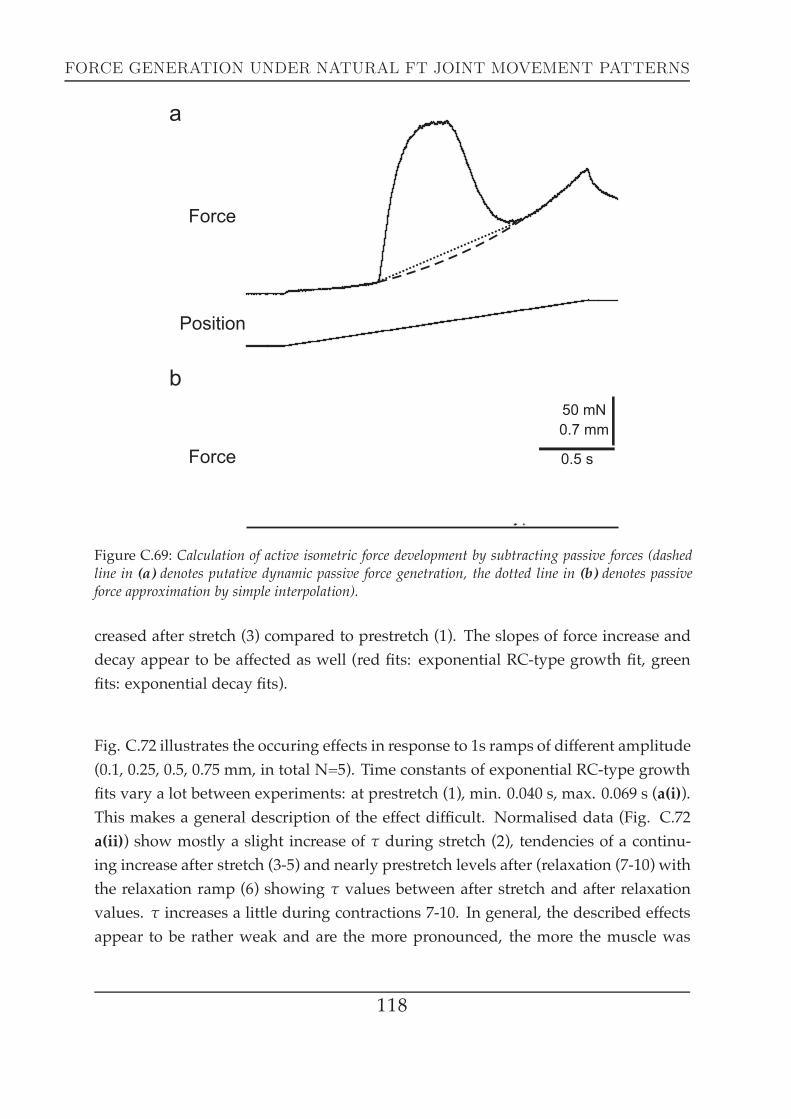
FORCE GENERATION UNDER NATURAL FT JOINT MOVEMENT PATTERNS

50 mN

0.7 mm

0.5 s

Force

Force

Position

a

b

Figure C.69: Calculation of active isometric force development by subtracting passive forces (dashedline in (a) denotes putative dynamic passive force genetration, the dotted line in (b) denotes passiveforce approximation by simple interpolation).

creased after stretch (3) compared to prestretch (1). The slopes of force increase anddecay appear to be affected as well (red fits: exponential RC-type growth fit, greenfits: exponential decay fits).

Fig. C.72 illustrates the occuring effects in response to 1s ramps of different amplitude(0.1, 0.25, 0.5, 0.75 mm, in total N=5). Time constants of exponential RC-type growthfits vary a lot between experiments: at prestretch (1), min. 0.040 s, max. 0.069 s (a(i)).This makes a general description of the effect difficult. Normalised data (Fig. C.72a(ii)) show mostly a slight increase of τ during stretch (2), tendencies of a continu-ing increase after stretch (3-5) and nearly prestretch levels after (relaxation (7-10) withthe relaxation ramp (6) showing τ values between after stretch and after relaxationvalues. τ increases a little during contractions 7-10. In general, the described effectsappear to be rather weak and are the more pronounced, the more the muscle was

118

RESULTS

0

20

40

60

80

100

120

140

160

180

0.5 0.6 0.7 0.8 0.9 1 1.1 1.2

Forc

e[m

N]

Time [s]

MeasuredFit increasing part

Fit decreasing part

5% Pmax

95% Pmax

Figure C.70: Calculation of the exponential RC-type growth (A = A0(1− e−tτ ) fits and exponential

decay A = A0e−tτ ) fits starting at 5% Pmax and 95% Pmax respectively, indicated by two ovals.

stretched.

This is different for relaxation phase time constants: prestretch values are much lessscattered (min. 0.055 s, max. 0.066 s) and muscle stretch causes are very distinct in-crease in all experiments (Fig. C.72b(i)). Relaxation causes in turn a very clear dropto prestretch levels. After relaxation, τ remains rather stable with a little tendencyto decrease at small stretch (0.1, 0.25 mm) and to increase at larger stretch (0.5, 0.75mm). As described for the force increase time constant, effects are more distinct, themore the muscle was stretched (comparing the green data points (0.75 mm ramp am-plitude) with the light blue ones (0.1 mm ramp amplitude) in b(ii)).

The course of Pmax can be very well described with the charcteristica presented inchapters C4 and C5: prestretch Pmax shows the large variation between animals thatwas already described in previous chapters (min. 99.45 mN, max. 156.01 mN, Fig.

119

FORCE GENERATION UNDER NATURAL FT JOINT MOVEMENT PATTERNS

0.25 s

50 mN

1

2

3

Figure C.71: Overlayed isometric contractions 1, 2 and 3 and their fits. Red solid lines denote expo-nential RC-type growth fits, green solid lines denote exponential decay fits.

C.72c(i)). Muscle stretch causes an immediate increase of Pmax because of the negativeshortening (i.e. ‘positive lengthening´) velocity applied to the muscle during contrac-tion. The double hyperbolic characteristic shown in Fig. C.52 predicts an increaseof 50 % when muscle is lengthened with velocities between 0.25 to 0.75 mm

s . This isexactly what happens: the higher the lengthening velocity, the bigger the increase ofPmax (datapoints at (2) in c(ii)). After stretch, Pmax remains rather stable at the samePmax-level following the force-length characteristic (chapter C2): 0.25 mm stretch elic-its the largest increase, 0.5 mm stretch causes already a slight Pmax decrease. This iswhat data in Figs. C.23 and C.24 in chapter 4 would predict because of the descendinglimb of the force-length relationship. This becomes evenmore distinct at larger stretch(0.75 mm): Pmax is decreased to about 50 %. During and after relaxation, Pmax-valuesare approximately at prestretch levels, with a tendency to increase slightly when pre-viously applied stretch amplitude was large (green and red trace in c(ii).

120

RESULTS

Figure C.72: Time constants of RC-type growth (a(i) and a(ii)), exponential decay (b(i) and b(ii)) andPmax (c(i) and c(ii)) at different muscle lengths (see Fig. C.68). Ramp amplitudes depicted in a(i) aslegend: 0.1 to 0.75 mm. Left column depicts absolute data values, right column shows data that werenormalised to prestretch values. All stretch and relaxation ramps had a duration of 1 s.

121

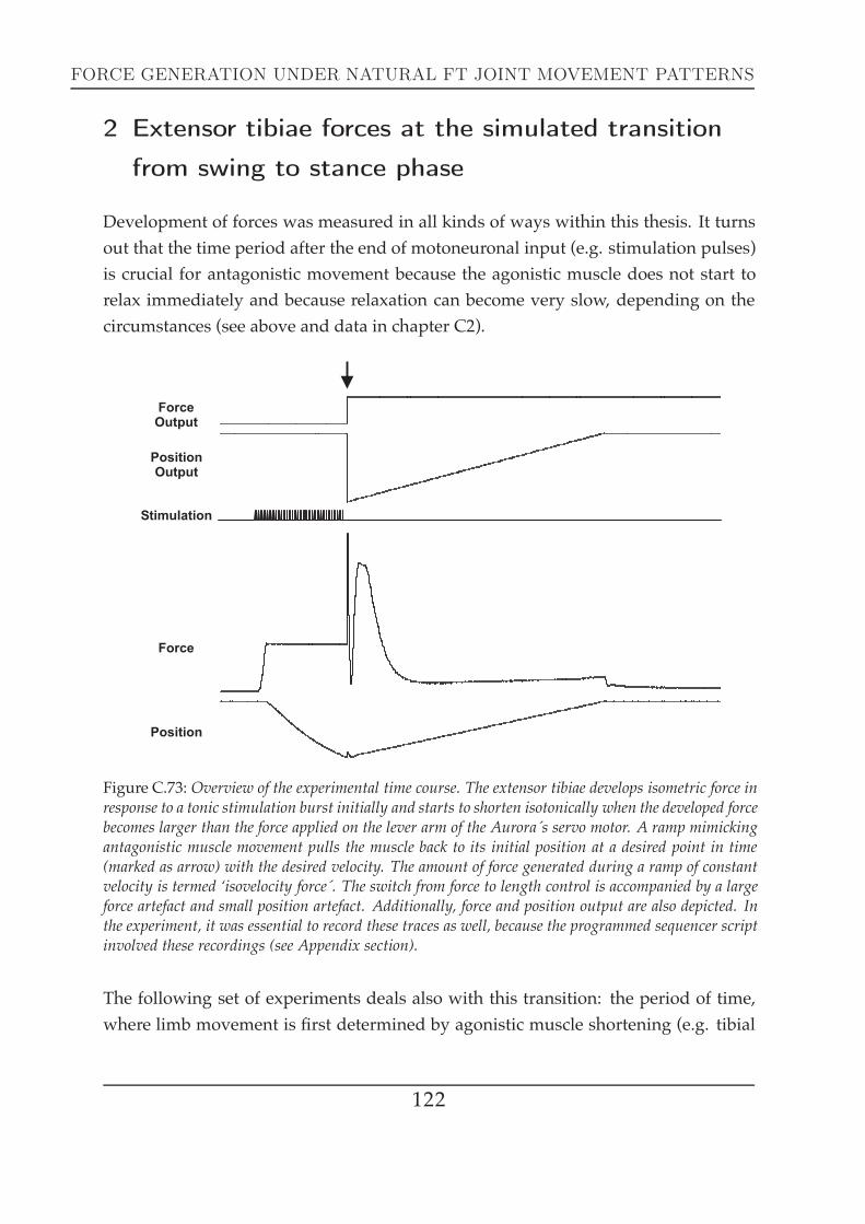
FORCE GENERATION UNDER NATURAL FT JOINT MOVEMENT PATTERNS

2 Extensor tibiae forces at the simulated transitionfrom swing to stance phase

Development of forces was measured in all kinds of ways within this thesis. It turnsout that the time period after the end of motoneuronal input (e.g. stimulation pulses)is crucial for antagonistic movement because the agonistic muscle does not start torelax immediately and because relaxation can become very slow, depending on thecircumstances (see above and data in chapter C2).

ForceOutput

PositionOutput

Stimulation

Force

Position

Figure C.73: Overview of the experimental time course. The extensor tibiae develops isometric force inresponse to a tonic stimulation burst initially and starts to shorten isotonically when the developed forcebecomes larger than the force applied on the lever arm of the Aurora´s servo motor. A ramp mimickingantagonistic muscle movement pulls the muscle back to its initial position at a desired point in time(marked as arrow) with the desired velocity. The amount of force generated during a ramp of constantvelocity is termed ‘isovelocity force´. The switch from force to length control is accompanied by a largeforce artefact and small position artefact. Additionally, force and position output are also depicted. Inthe experiment, it was essential to record these traces as well, because the programmed sequencer scriptinvolved these recordings (see Appendix section).

The following set of experiments deals also with this transition: the period of time,where limb movement is first determined by agonistic muscle shortening (e.g. tibial

122

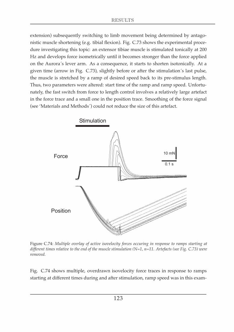
RESULTS

extension) subsequently switching to limb movement being determined by antago-nistic muscle shortening (e.g. tibial flexion). Fig. C.73 shows the experimental proce-dure investigating this topic: an extensor tibiae muscle is stimulated tonically at 200Hz and develops force isometrically until it becomes stronger than the force appliedon the Aurora´s lever arm. As a consequence, it starts to shorten isotonically. At agiven time (arrow in Fig. C.73), slightly before or after the stimulation´s last pulse,the muscle is stretched by a ramp of desired speed back to its pre-stimulus length.Thus, two parameters were altered: start time of the ramp and ramp speed. Unfortu-nately, the fast switch from force to length control involves a relatively large artefactin the force trace and a small one in the position trace. Smoothing of the force signal(see ‘Materials and Methods´) could not reduce the size of this artefact.

Figure C.74: Multiple overlay of active isovelocity forces occuring in response to ramps starting atdifferent times relative to the end of the muscle stimulation (N=1, n=11. Artefacts (see Fig. C.73) wereremoved.

Fig. C.74 shows multiple, overdrawn isovelocity force traces in response to rampsstarting at different times during and after stimulation, ramp speed was in this exam-

123

FORCE GENERATION UNDER NATURAL FT JOINT MOVEMENT PATTERNS

ple 0.66 mms (N=1, n=11). At ramp starts > 0.08 s after the last stimulation pulse, forcehas diminished almost completely.

Figure C.75: Maximally actively generated forces occuring in response to different ramp speeds withlinear fits. (a) 0.86 mms (dashed line, *** p < 0.001; N=1, n=12) and 0.66 mms (dotted line, *** p <0.001; N=1, n=11). (b) From one examplary animal (N=1): 0.33 mms (dashed-dotted line, ** p = 0.007,n=4), 0.66 mms (dashed line, * p = 0.013, n=4) and 1.32 mms (dotted line, * p = 0.010, n=4). Allstimulations consisted of 50 pulses at 200 Hz.

Fig. C.75 shows evaluations of experiments, where ramps were started throughoutthe second half of stimulation (-0.15 s to 0 s (a)) and after the stimulation until ramp

124

RESULTS

stretch could not anymore elicit any measureable forces (0 s to 0.08 s, (b)). Time =0 s corresponds to the time of the last stimulation pulse in each single experiment.The earlier the ramp start, the larger the maximal force response (Pmax). After stim-ulation, force occurence arises from the slow force decrease of isotonic contractions(Hooper et al. (2007a)) combined with the effect of lengthening a muscle that still triesto shorten further, see Hill characteristics at negative contraction velocities (chapterC4). This characteristic explains Pmax to be larger at faster ramps mimicking fasterstance phases (see C.75b). The faster the ramp, the steeper the slope of the linear datafits (−0.493 mNms at 0.33

mms , −0.567

mNms at 0.66

mms and −0.689 mNms at 1.32

mms ). Up to 75

ms after the last stimulation pulse, the extensor tibiae shows force development in re-sponse to a ramp resetting the muscle to its original position. After 80 ms, the muscleceases to generate force, even when being stretched with the fastest ramp (1.32 mms ).

From the insights gained in chapter C3 (that passive muscle forces can play a majorrole), it was necessary to look at the passive dynamic force development involvedas well. Fig. C.33 demonstrated that passive dynamic forces of extensor and flexortibiae can become remarkably large (> 50 mN when stretched fast starting at 90° FTjoint angle). Passive force responses to the same ramp stretch velocities which wereused in Fig. C.75b (0.33 mms , 0.66

mms , 1.32 mms ) are displayed in Fig. C.76: maximal

dynamically generated force was 6.26 ± 0.31 mN (N=1, n=5) in response to the fastestramp.

0.2 s

0.2 mm2 mN

Passiveforce

Position

Figure C.76: Multiple overlay of passive isovelocity forces occuring in response to ramps of differentspeed (0.33 mms , 0.66

mms , 1.32 mms ).

125

FORCE GENERATION UNDER NATURAL FT JOINT MOVEMENT PATTERNS

3 Interaction of agonistic and antagonistic passivelyand actively generated forces during simulatedswing and stance

Chapters C2-C5 dealt with the descriptions of either isometric passive, isometric ac-tive, isotonic passive or isotonic active forces. Measurements were all done by di-rectly measuring at the muscle (either extensor or flexor tibiae) and different issueswere highlighted in a very isolated way. In order to get a broader picture, the follow-ing experiments were conducted while leaving the whole middle leg intact, either theextensor tibiae nerve nl3 or the flexor tibiae nerve ncr were stimulated with 200 Hzand tibia movement dynamics were tracked with a highspeed camera (see ‘Materialsand Methods´ section).

3.1 Simulating tibial swing / stance phase

Different numbers of pulses were tested and FT joint angular displacements weretracked vs. time. Fig. C.77 illustrates the fast tibial movement beginning in all experi-ments at 0.06 s, i.e. 0.01 s after stimulation begin (the first 50 ms tracked the resting legbefore stimulation begin). This is consistent with the twitch latency determinationsshown in Tabs. C.3 and C.4. Initial tibia position in extensor tibiae experiments wasfound to be 102.2 ± 0.3° (N=1, n=3) and 88.6 ± 2.9° (N=1, n=3) in flexor tibiae experi-ments. A paired t-test showed the values to be significantly different from each other(*, p < 0.02). Thus, as antagonistic innervation was either crushed or cut (seeMaterialsand Methods section), the lack of antagonistic tonic motoneuronal firing seems to havean impact on tibia rest position. Either when the extensor tibiae was silent (resultingin a more flexed tibia rest position) or when the flexor tibiae was silent (resulting in amore extended tibia rest position). The tibia appears to be extended and flexed withapproximately the same speed because the individual angular increasing (at extensortibiae stimulation) and angular decreasing phases (at flexor tibiae stimulation) in Fig.C.77a parallel each other until the maximal deflection is reached for each stimulation.This maximal deflection is 30° to 180°, which is consistent with the maximal physio-logical working range (see above). At stimulation of both extensor and flexor tibiae,relaxation (i.e. when the tibia starts to return to its rest position) after 20 pulse stimu-lation starts after the same time t1 (see Fig. a). When a maximal angle is reached and

126

RESULTS

the tibia cannot be extended or flexed further, the tibia remains at the same positionand starts to relax when stimulation is over (extensor tibiae at 40 pulses and flexortibiae at 30 pulses).

Figure C.77: Video analysis of tibia movement during and after 200 Hz stimulation of either extensor(N=1; 15, 20, 40 pulses) or flexor tibiae (N=1; 10, 20, 30 pulses). (a) Absolute tibial deflections overtime. t1 marks relaxation starts after 20 spike duration of extension and flexion repectively and t2 aftermaximal extension and flexion. (b) Relative angular displacement over time. Numbers in red denotestimulation pulse number. The relaxation start of the stimulated muscle (i.e. when the tibia starts toreturn to its rest position) is consistent with the stimulation pulse number, no matter what muscle(extensor or flexor tibiae) was activated.

127

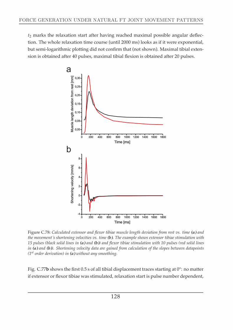
FORCE GENERATION UNDER NATURAL FT JOINT MOVEMENT PATTERNS

t2 marks the relaxation start after having reached maximal possible angular deflec-tion. The whole relaxation time course (until 2000 ms) looks as if it were exponential,but semi-logarithmic plotting did not confirm that (not shown). Maximal tibial exten-sion is obtained after 40 pulses, maximal tibial flexion is obtained after 20 pulses.

Figure C.78: Calculated extensor and flexor tibiae muscle length deviation from rest vs. time (a) andthe movement´s shortening velocities vs. time (b). The example shows extensor tibiae stimulation with15 pulses (black solid lines in (a) and (b)) and flexor tibiae stimulation with 10 pulses (red solid linesin (a) and (b)). Shortening velocity data are gained from calculation of the slopes between datapoints(1st order derivation) in (a) without any smoothing.

Fig. C.77b shows the first 0.5 s of all tibial displacement traces starting at 0°: no matterif extensor or flexor tibiae was stimulated, relaxation start is pulse number dependent,

128

RESULTS

i.e. post-flexion relaxation after 10 pulses starts before post-extension relaxation after20 pulses etc. Time courses of tibial angular displacement at extensor tibiae stimula-tion with 15 pulses and of flexor tibiae stimulation with 10 pulses are rather similar(see Fig. C.77b), but the actual calculated muscle length changes vs. time for bothmuscles under consideration of their individual moment arm lengths look very dif-ferent (Fig. C.78a).

The flexor tibiae experiences a much larger length change than the extensor tibiae butpeaks at nearly the same time. Thus, themean shortening velocity of the flexor tibiaeis supposed to be twice as large compared to the extensor tibiae when its momentarm is twice as long. Nonetheless, the maximal calculated shortening velocities ofextensor and flexor tibiae can vary far more than twofold, which is illustrated in Fig.C.78b: the flexor tibiae reaches a maximum velocity of 8.34 mms after 100 ms and theextensor tibiae reaches a maximum velocity of 2.61 mms after 120 ms.

3.2 Simulated swing relaxation at maximal tibia extension

The next approach was to test whether pulse number has an impact on the tibialreturn dynamics after extension, given the maximal tibial extension angle is the sameat all stimulations. Stimulation consisted of either 20, 40, 60, 80, 100, 120 or 140 pulsesat 200 Hz with the antagonist´s nerve (ncr) being cut, a paradigm already used insection 1.4 of chapter C2. The idea was to stimulate the muscle long enough to makeit extend the tibia maximally (180°) and to stimulate it then even further. Fig. C.79ashows neither 20 pulse stimulation to be sufficient to extend the tibia maximally (max.angle 145°), nor 40 pulse stimulation (max angle 176°). 60 pulses and more led to acomplete extension and even further. Interestingly and not expected, the tibia can beextended more than 180° when stimulation is continuing (maximally 184°). In Fig.C.79b, tibia movement is translated into extensor tibie muscle length (90° = rest angle= 0). Chapter C1 described the relation betweenmuscle length and joint angle in greatdetail and showed that muscle length deviated from the cosine course in the range ofextreme angles, i.e. 30° and 180°. This deviation is necessary because the joint wouldnot be able to move if the two limbs of a joint (femur and tibia) were in line with theoperating force vectors (‘mechanical dead centre´). As the tibia can hardly be returnedin such extreme positions (175-185°, Fig. C.79a), the different relaxation time courses

129

FORCE GENERATION UNDER NATURAL FT JOINT MOVEMENT PATTERNS

in response to different stimulation durations depicted in Fig. C.79a and b are hard tointerpret because it is not clear whether this movement dynamics effect comes fromthe fact that the joint is close to being in a dead centre or whether this effect arisesfrom the increasing τ described in chapter C2.

a

0 100 200 300 400 500 60090

100

110

120

130

140

150

160

170

180

Time after last pulse [ms]

FT-a

ng

le[°

]

b

Mu

scle

len

gth

de

via

tion

fro

mre

st[m

m]

0 100 200 300 400 500 6000.00

0.05

0.10

0.15

0.20

0.25

0.30

20 pulses20 pulses406080100120140

Time after last pulse [ms]

Figure C.79: (a) FT joint angle plotted over time after the last 200 Hz stimulation pulse (pulse numberlegend is displayed as well). Additionally (b), extensor tibiae muscle length was plotted vs. time underconsideration of extensor tibiae moment arm length (0.282 mm, see chapter C1). Moment arm lengthwas calculated to be maximal at 185°: 5° were subtracted from all calculated joint angles because of themuscle being close to a mechanical dead centre (see text for details).

3.3 Simulated swing relaxation after hitting an obstacle

As could already be demonstrated in chapter C2, different stimulation durations havean impact on the subsequent muscle relaxation phase and on the delay of this relax-ation in the isometric domain. The above described experiments attempted to test thisaspect on a more physiological level, i.e. a real tibia movement. The aim of this studywas to look whether prolonged extensor tibiae activity is reflected not only in longermuscle relaxation, but also in longer tibia restoring dynamics. As middle leg swingphases vary in the number of action potentials generated by the FETi motoneuron(see chapter 4), it needs to be clarified to which extent the subsequent tibia move-ment dynamics are biased by this fact. The previous examination (Fig. C.79a and b)could not satisfactorily answer this question, because maximal possible tibia exten-sion involves mechanical difficulties that complicate interpretation of the results (seeabove). In order to overcome the difficulties of a mechanical dead centre, the exper-

130

RESULTS

imental approach was slightly changed in the following investigation. In contrast tothe previous study, extreme tibia extension (> 140° FT joint angle) was blocked witha heavy pen (Faber-Castell) mounted on a micromanipulator (see Fig. C.80, exp. 1).With this setting, the tibia position from which the tibia restoring process started wasalways the same, no matter how long the extensor tibiae muscle was stimulated. Thestimulation paradigm was the same as in the previous section.

Extensorstimulation

Extensoractive force

Flexorpassive force

Flexorstrain

35 ms

20 mN

50 mN

2 mm

0.2 s

Beforestimulation

Beforestimulation

Duringstimulation

Duringstimulation

Experim

ent1

Experim

ent

1E

xperim

ent2

Experim

ent

2E

xperim

ent3

Experim

ent

3

Figure C.80: Combination of three kinds of experiments: (exp. 1) High-speed video tracking of tibiamovement achieved by 200 Hz extensor tibiae stimulation of different duration (20-140 pulses). Ex-treme tibia movement is blocked by a heavy pen (Faber-Castell). Two still photographs are shown: beforestimulation begin and during stimulation when the tibia is blocked by the pen. (exp. 2) Isometric forcemeasurement at 200 Hz stimulation of different duration (20-140 pulses). (exp. 3) Measuring passiveflexor tibiae force by muscle stretch mimicking tibia movement in amplitude and duration (0.28 mm in0.09 s, adjusted amplitude and time to exp.1). Exps. (2) and (3) are on the same time scale, the dashedlines indicate time after the stimulation end at 20 and 140 pulses as well as 35 ms after, as this was therelaxation movement begin at all stimulations.

131

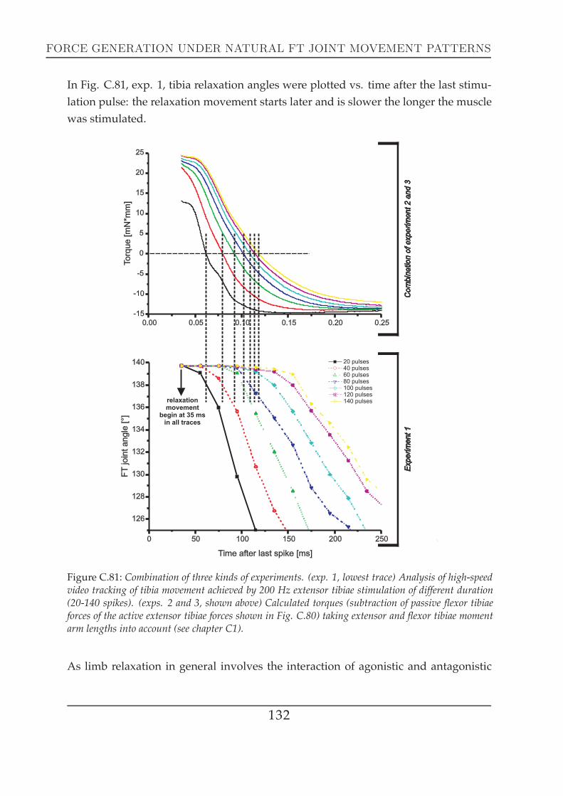
FORCE GENERATION UNDER NATURAL FT JOINT MOVEMENT PATTERNS

In Fig. C.81, exp. 1, tibia relaxation angles were plotted vs. time after the last stimu-lation pulse: the relaxation movement starts later and is slower the longer the musclewas stimulated.

Figure C.81: Combination of three kinds of experiments. (exp. 1, lowest trace) Analysis of high-speedvideo tracking of tibia movement achieved by 200 Hz extensor tibiae stimulation of different duration(20-140 spikes). (exps. 2 and 3, shown above) Calculated torques (subtraction of passive flexor tibiaeforces of the active extensor tibiae forces shown in Fig. C.80) taking extensor and flexor tibiae momentarm lengths into account (see chapter C1).

As limb relaxation in general involves the interaction of agonistic and antagonistic

132

muscles, isometric extensor tibiae force at 200 Hz stimulation of different duration(20-140 spikes) was measured (Fig. C.80, exp. 2) and, additionally, the flexor tibiaewas stretched with a rampmimicking tibia extension amplitude and duration trackedby the camera (Fig. C.80, exp. 3). With the intention to reconstruct tibial relaxationdynamics, subtractions of passive flexor torques from the active extensor torques aredisplayed in Fig. C.81, the combination of exps. 2 and 3. Comparison of the timeswhere the individual torque traces cross 0 mN*mmwith the movement traces shownunderneath (Fig. C.81, exp. 1) shows satisfying accordance. The stimulation-historydependent effect being an intrinsic property of the extensor tibiae affects the differenttibial movement return dynamics. Magnitude and time course of passive flexor forcesgive a good reference point in order to understand the actual begin of relaxation.

133

D. Discussion

134

Biomechanical muscle investigations were performed in order to characterise mainlythe extensor tibiae, and in parts the flexor tibiae, of the stick insect Carausius morosus.The basic idea of these examinations consisted in the desire to understand the oper-ation of a neuromuscular system (i.e. examining motoneuron output and muscularproperties in a functional context) by taking a simply innervated leg muscle (Blick-han et al. (2003); Hooper and Weaver (2000)). The need for this investigation wasparticularly high as the stick insect presents a very well explored system in terms ofmotoneuronal activity, however as yet little is known on the direct translation of mo-toneuronal action potentials into muscle activity with an exception for muscle forcegeneration in response to chordotonal organ stimulation (Storrer (1976); Storrer andCruse (1977); Bässler and Stein (1996)). The extensor tibiae is a particularly good can-didate, as it is innervated by just three motoneurons (Bässler and Storrer (1980)), butalso well understood in lots of aspects: its pattern of muscle fibre innervation (Bässlerand Stein (1996)) and muscle fibre composition (Bässler et al. (1996)), its role in rock-ing behaviour (Pflüger (1977)), or its role as an effector in response to local feedbackfrom sensory neurons about movements (e.g. Bässler (1967); Bässler and Büschges(1998); Büschges (2005)) or forces (e.g. Akay et al. (2001); Akay and Büschges (2006)).Most biomechanical investigations are either focussed on one topic like e.g. the force-velocity relationship (Edman (1988)) or they are performed on muscles not being in-volved in leg movement (typically flight muscles, like e.g. Machin and J. W. Pringle(1960);Malamud (1989);Malamud and Josephson (1991)). This thesis presents a broadinsect leg muscle description that comprises examinations on many muscle physi-ological and biomechanical aspects. The richness of muscle data from over half acentury (e.g. Hill (1938)) allows classification and comparison to other muscle-jointsystems. The data gathered within this thesis provide enough aspects to begin mod-elling the muscle with more than 20 parameters (Ekeberg et al. (2004); Blümel et al.(2007a;b; 2008b;a)). Experiments mimicking physiological motoneuronal firing pat-terns further deepened the understanding of the extensor tibiae´s role in behaviour(Hooper et al. (2006; 2007a;b)).

135

FEMORAL GEOMETRY

D1 Femoral geometry

SummaryThere is a clear linear dependence between femur length and muscle length of ex-

tensor and flexor tibiae for all three legs, tibial front leg muscles are notably shorter. Itwas shown that extensor tibiae muscle length changes with the cosine of the FT jointangle and flexor tibiae length changes with the negative cosine, except for extremeangles (close to 30° or 180°). Flexor tibiae moment arm length of all three legs (0.564mm) is twice the moment arm length of all three legs´ extensor tibiae muscles (0.282mm). Proximal and medial flexor tibiae fibres are approximately 1.5 times longer(2.11 mm) than proximal and medial extensor tibiae fibres (1.41 mm). Preliminaryphalloidin stainings could show that the percental length changes that extensor andflexor tibiae fibres experience within the muscles´ working range of 150° deviate fromthe percental sarcomere length changes for their sarcomeres. Standardisation of sar-comere lengths result in means of 5.4 µm for the extensor and 6.9 µm for the flexortibiae. Further examination is required in order to make a clear statement to this is-sue. Femoral cross-sectional area is about 0.5 mm2 and extensor tibiae cross-sectionalarea about 1.9 mm2.

DiscussionRandomly picked sturdy looking female stick insects had body masses around 1 g

(0.94 ± 0.07 g, N=10) and body lengths of 77.1 ± 2.28 mm (N=10), about the same val-ues found by Burrows and Wolf, 1.1 ± 0.004 g and 78 ± 0.15 mm (N=10, Burrows andWolf (2002)). The small inter-animal variation (small S.D. values) and the similarityto the values of another institute´s breeding suggests stick insects from the Cologneinstitute´s breeding to be representative for muscle examinations. This fact is particu-larly important in respect to the issue of data variability, see chapters D2 and D4. Theproportion of relative femur lengths of the three legs presented in chapter C1 alignedwith the findings from Burrows and Wolf: front leg femur is the longest, hind leg fe-mur almost as long andmiddle leg femur about 23 the front leg femur length (Burrowsand Wolf (2002)).

136

DISCUSSION

Flexor and extensor tibiae muscle rest lengths of all three legs were shown to be pro-portional to femur length (see Fig. C.1). The specialisation of the front legs causestibial muscles to fill out only three quarters of the femur length (76 % for the extensortibiae and 73 % for the flexor tibiae, see Tab. C.1). Stick insects have a narrow, redcoloured femur base in each front leg that allows them to hold their front legs ros-trally over the animal’s head and thus to mimic twigs (Marquardt (1940); Bässler andWegner (1983). Opening the proximal femur reveals no tibial muscle fibres to be inthe proximal part.

Investigating the dependence of muscle length on joint angle is considerably simpli-fied by the fact that arthropod apodemes are 40 times as stiff as mammalian tendons(Ker (1977); Full and Ahn (1995); Full et al. (1998)) as this allows an unambiguous re-lation. Taking the muscle reference length as the muscle length when its moment armis perpendicular to the long axis of the segment comprising the muscle in focus (Fullet al. (1998)), in this case the femur, seemed to be reasonable although this may not bethe actual ‘rest length´. The real ‘rest length´ is likely to be different for every individ-ual muscle and would have required cutting the distal apodeme at the beginning ofeach experiment and looking to which length the muscle shrinks.

The deviations of normalised muscle length (see Fig. C.2) changes from a fitted cosinefunction (and the negative cosine function respectively) that can be found in the ex-tensor tibiae (and flexor tibiae respectively) can be interpreted simply by consideringmechanical laws and truely make sense as the muscle would be unable to move thetibia out of extreme positions (where these deviations occur, e.g. during thanatosis(Bässler (1972); Godden (1974)). The fitted cosine function does not properly describethe range of angles close to the endpoint at 180°, the values still show a slope differentfrom zero and not a horizontal tangent as would be described by a cosine function.This avoids the problems of amechanical dead point for the tibial muscles at extendedjoint angles. Within the range of joint angles occuring inmost physiological situations,the relationships between joint angle and muscle length were approximately linear,very similar to data shown for cockroach (Blaberus discoidalis) extensor muscles of allthree segments (muscles 87 (prothoracic), 137 (mesothoracic) and 179 (metathoracic),Full et al. (1998)). It has to be mentioned that the moment arm orientation arrange-ment of extensor and flexor tibiae was not explicitely checked. The assumption made

137

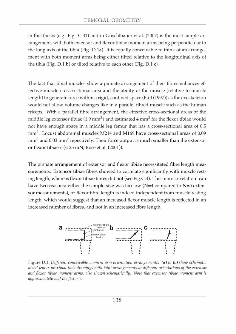
FEMORAL GEOMETRY

in this thesis (e.g. Fig. C.31) and in Guschlbauer et al. (2007) is the most simple ar-rangement, with both extensor and flexor tibiae moment arms being perpendicular tothe long axis of the tibia (Fig. D.1a). It is equally conceivable to think of an arrange-ment with both moment arms being either tilted relative to the longitudinal axis ofthe tibia (Fig. D.1 b) or tilted relative to each other (Fig. D.1 c).

The fact that tibial muscles show a pinnate arrangement of their fibres enhances ef-fective muscle cross-sectional area and the ability of the muscle (relative to musclelength) to generate force within a rigid, confined space (Full (1997)) as the exoskeletonwould not allow volume changes like in a parallel fibred muscle such as the humantriceps. With a parallel fibre arrangement, the effective cross-sectional areas of themiddle leg extensor tibiae (1.9 mm2) and estimated 4 mm2 for the flexor tibiae wouldnot have enough space in a middle leg femur that has a cross-sectional area of 0.5mm2. Locust abdominal muscles M214 and M169 have cross-sectional areas of 0.09mm2 and 0.03 mm2 repectively. Their force output is much smaller than the extensoror flexor tibiae´s (< 25 mN, Rose et al. (2001)).

The pinnate arrangement of extensor and flexor tibiae necessitated fibre length mea-surements. Extensor tibiae fibres showed to correlate significantly with muscle rest-ing length, whereas flexor tibiae fibres did not (see Fig.C.4). This ‘non-correlation´ canhave two reasons: either the sample-size was too low (N=4 compared to N=5 exten-sor measurements), or flexor fibre length is indeed independent from muscle restinglength, which would suggest that an increased flexor muscle length is reflected in anincreased number of fibres, and not in an increased fibre length.

Figure D.1: Different conceivable moment arm orientation arrangements. (a) to (c) show schematicdistal femur-proximal tibia drawings with joint arrangements at different orientations of the extensorand flexor tibiae moment arms, also shown schematically. Note that extensor tibiae moment arm isapproximately half the flexor´s.

138

DISCUSSION

Flexor tibiae fibres are nearly 1.5 times longer than extensor tibiae fibres. This findingbecomes particularly important with respect to the maximum contraction velocity afibre can bear, as it is dependent on its sarcomere number (Huxley and Niedergerke(1954a); Thuma (2007)) and will therefore be discussed below. The physiological sig-nificance of proximal extensor tibiae fibres being longer than medial ones and proxi-mal flexor tibiae fibres being shorter thanmedial ones remains unclear. Determinationof pinnation angles (see in theResults section) led to the conclusion, that measurementof fibre length changes is afflicted with an error of less than 3 % when calculated witha pinnation angle of zero, i.e. as if the fibre were arranged parallel to the muscleapodeme for both tibial muscles. Consistent with this calculation, a parameter studyto calculate extensor mass of the dinosaur Tyrannosaurus showed that altering pinna-tion angle within a reasonable range of values had little or no effect (Hutchinson andGarcia (2002)).

The flexor tibiae´s moment arm being twice as long as the extensor tibiae´s seems tobe an adaptation to the flexor´s longer fibres (see Fig. C.3): extensor and flexor tibiaeexperience similar relative fibre length changes during walking. The middle leg flexortibiae is mainly active during stance phase (Fischer et al. (2001); Schmidt et al. (2001);Gabriel et al. (2003)), it profits of a longer moment arm length in order to generatelarger torques. The extensor tibiae in turn can take advantage of a shorter momentarm length in order to accomplish fast movements during swing phase (Bässler andBüschges (1998); Graham (1985)). Interestingly, middle leg extensor tibiae momentarm length can be very different in orthopteran insects, as femoral chordotonal or-gan apodeme movement of 0.2 mm in Carausius morosus (Weiland et al. (1986)), 0.4mm in Cuniculina impigra and 0.6 mm in Locusta migratoria (Field and Pflüger (1989))corresponds to a joint angle change of 40°, respectively (Bässler et al. (1996)). The de-termination of Weiland and colleagues (Weiland et al. (1986)) in Carausius morosus isin very good agreement with the examinations in this thesis: the same angular deflec-tion of 40° around a centre position of 90° (like they did) results in an extensor tibiaeexcursion of 0.19 mm, when calculated with a moment arm length of 0.282 mm.

Sarcomere length measurements were conducted in order to answer two questions:Do sarcomeres of extensor and flexor tibiae experience the same percent length changesas do the fibres of both muscles? Do extensor and flexor tibiae sarcomeres differ in

139

FEMORAL GEOMETRY

their structural arrangement? Nissl sarcomere stainings of the extensor tibiae weredifficult to interpret, because the procedure involved too many unpredictable factors(e.g. distortion of the material after paraffin treatment). As the quality of the stain-ings was not too good, the descision was made to take phalloidin as a classic musclestructure fluorescent dye. The outcome of these stainings was much better in qualityand the sarcomere length changes quite close to the range of length changes that canbe expected from the calculated fibre length changes. The fact that extensor tibiae sar-comeres experience 25 % less length change than the fibres and flexor tibiae sarcom-eres experience 13 %more length change suggests that there could be some structuralelements that cause this mismatch. For example, it is conceivable to think about theexistence of proteins that connect the fibre with the cuticle or with the tendon. Theseproteins could cause only a few components of the fibre (e.g. some sarcomeres) tostretch more or less than the entirety of the fibre: this would necessarily lead to a cer-tain mismatch. It was already discussed (see above in this ‘Discussion´ chapter) thatmuscle lengths show deviations from the cosine characteristic at extreme angles like30° and 180° and that these deviations make sense from a physiological aspect. It istherefore also conceivable to trace the mismatch found between the calculated lengthchanges of fibres and the measured length changes of sarcomeres back to the devia-tion from the cosine course.

The second issue to be solved with sarcomere length data concerned the comparisonof the general structure of sarcomeres in different muscles. The standardisation tech-nique by Thuma and colleagues (Thuma (2007); Thuma et al. (2007)) represents an ap-propriate tool to conduct this comparison. They compared different pyloric and gas-tric mill muscles in the lobster Panulirus interruptus and found large variability withina pool of nine muscles: the structure of sarcomeres can vary extremely between mus-cles accomplishing similar functions. The result of the standardisation procedure isto reduce each sarcomere to two times its thin filament length. The fact that standard-ised sarcomere lengths from a muscle fixed at 30° and from a muscle fixed at 180° arewithin a similar range, but still significantly different from one another again suggeststhat the existence of e.g. elastic proteins being responsible for the detected mismatchis likely. The examination revealed middle leg mean tibial sarcomere lengths of 5.42µm for the extensor and 6.93 µm for the flexor tibiae (see Figs. C.5, C.6, C.7). Thuma(Thuma (2007)) investigated sarcomere lengths of nine muscles in the lobster stom-atogastric system that have standardised lengths ranging from 3.25 µm to 12.29 µm

140

DISCUSSION

with four muscles having a length between 5 and 8 µm, similar to standardised tibialmuscle sarcomere lengths. Other sarcomere lengths found: 2.20 µm (anterior tibialismuscle of Rana temporaria, Edman (2005)), 2.6-2.7 µm (flexor digitorum brevismuscle ofthe mouse), 2.45 µm (semitendinosusmuscle of Rana temporaria, Edman (1966)), 2.5 µm(psoasmuscle of the rabbit, Ranatunga et al. (2007)), 2.5 µm (flexor halucis brevismuscleof the rat, Roots et al. (2007)), 2.58 and 2.71 µm (soleus and extensor digitorum longusmuscle in the mouse). The standardised sarcomere lengths of extensor and flexor tib-iae are within the same ballpark than many other arthropod sarcomeres, however adirect comparison is impossible because the precise contraction state of each sarcom-ere is unknown. In general, longer sarcomeres with longer myosin filaments are capa-ble of generating greater stress (Full and Ahn (1995)). This is confirmed by examina-tions on different crab closer muscles that revealed sarcomere lengths between 10 and18 µm (Taylor (2000)). Taylor describes a linear relationship between resting sarcom-ere length and maximum muscle stress including arthropods (without crustaceans),crustaceans and vertebrates: the longer the sarcomere, the larger the maximum stress(Taylor (2000)). From this regression, tibial muscles should exert as much as 350 - 400kNm2 in respect to their calculated standardised sarcomere lengths. However, maximalextensor tibiae stress is 79 ± 23 kNm2 (N=7, see Tab. C.7) and maximal flexor tibiae stressis 104 ± 32 kN

m2 (N=8, see Tab. C.8): both tibial muscles deviate from this regressionand exert less stress than expected. Apart from maximum muscle stress generation,another important parameter in terms of the functional relevance of sarcomeres isthe maximal shortening velocity (V0), which is supposed to be dependent on sarcom-ere number, as Huxley andNierdergerke (Huxley andNiedergerke (1954a)) predictedand later Thuma (Thuma (2007); Thuma et al. (2007)) showed. For both tibial muscles,sarcomere number can be calculated as follows: ( f ibre length at a particular contraction state)

(sarcomere length at a particular contraction state)= (sarcomere number at particular contraction state). For the extensor tibiae, the ratiois 1.65mm7.50 µm = 220 at 30° FT joint angle and

1.13mm6.21 µm = 182 at 180° ( see Tab. C.2). For the

flexor tibiae, the ratio is 1.62mm5.16 µm = 314 at 30° FT joint angle and2.67mm9.16 µm = 291 at 180° (see

Tab. C.2). Taking the means for both muscles gives ∼ 200 sarcomeresf ibre for the extensor

tibiae and ∼ 300 sarcomeresf ibre for the flexor tibiae. Consequently, the sarcomere number

predicts V0 of the flexor tibiae to be about 1.5 times larger than V0 of the extensor tib-iae. Quick release experiments prove this predictions to hold true (compare Tabs. C.7with C.8 in chapter C4): the ratio V0 o f the f lexor tibiae

V0 o f the extensor tibiae is with 1.38 close to the predictedvalue, calculated with 6.05 mm

s for the flexor tibiae (N=8) and 4.39 mms for the exten-

sor tibiae (N=7). Although these data are intriguing, they should only be considered

141

FORCE MEASUREMENTS IN THE ISOMETRIC DOMAIN

preliminary because they come from only two animals for each muscle.

D2 Force measurements in the isometric domain

SummaryExtensor tibiae single twitch force is notably smaller than maximal tetanic force (2-

6 mN compared to > 100 mN) and takes long to relax completely (> 140 ms). Flexortibiae twitch force can become remarkably big (> 30 mN), depending on the degreeof recruitment. These strong twitches show a steady amplitude decrease at conti-nous stimulation whose nature is unknown. Both increase in stimulation frequencyand stimulation duration have a positive impact on the persistence of maximal forcegeneration and on the relaxation decay dynamics in the extensor tibiae. The muscleappears to response to a short-term altering stimulation in frequency or pulse num-ber with an increased force level (‘catch-like effect´ or ‘latch´). Thus, the muscle cancompensate for stimulation intermissions to some extent. The extensor tibiae has itsworking range (30° to 180°, see also Friedrich (1932)) on the ascending limb of theforce-length relationship described by Gordon et al. (Gordon et al. (1966b)). The max-imally generated force was in most experiments shifted towards longer fibre lengthsat lower stimulation frequencies.

DiscussionThe method of examining forces the way it was done within this thesis differs es-

sentially from the usual way the forces of most vertebrate muscles (e.g. frog in Hill(1938) or Edman (1988)) are measured. Single fibre measurements are most oftenperformed on vertebrate muscle because their muscle fibre membranes normally fea-ture voltage-dependent Na+- channels and are therefore able to be stimulated whenplaced between two small metal discs, which is methodologically a big advantage,because parameters like temperature or application of drugs can be controlled moreaccurately, and the muscle can be stimulated directly and not via the nerve. This kindof stimulation is not possible in invertebrates. The experimentalist has basically twopossibilities: either eliciting motoneuronal action potentials with a monopolar suc-tion electrode (Grillner et al. (1998)) or with a bipolar electode. The main advantage

142

DISCUSSION

of the latter is that the generated electrical field is restricted to the nerve and the mo-toaxons therefore need presumably much less current to generate action potentials.Additionally, the fact that stick insect tibial muscles are pinnate and that single fibreforces are unmeasurably small make single fibre measurements inconceivable (at leastwith a force transducer like the Aurora 300 B dual-lever system). Apart from this as-pect, whole muscle measurements have a clear advantage compared to single fibremeasurements: it is very improbable that a muscle fibre, with a length hundreds oftimes its diameter, is supposed to have a constant strength throughout (Hill (1949)).In a whole muscle, with many fibres working in parallel, an average value is obtainedbeing much more constant than in a single fibre (Abbot and Aubert (1952)).

Extensor tibiae nerve stimulation (nl3) was set to an amplitude that elicited a visibletwitch in the force trace adding at least 50 %. With this stimulation, the FETi motoneu-ron was obviously excited and it is most likely to have activated the SETi and the CI1motoneuron simultaneously, a paradigm that comes close to the naturally ocurringactivation pattern during swing phase: excitatory and inhibitory extensor motoneu-rons are activated together with instantaneous frequencies of up to 200 Hz (Schmitzand Hassfeld (1989); Büschges (1995b); Kittmann et al. (1996)). Separate stimulationof individual excitatory motoneurons is not possible extracellularly (Bässler and Stor-rer (1980)). As was demonstrated in the Materials & Methods section (see also Fig.B.5), a set of 15 experiments was conducted to deal with the question whether si-multaneous activation was achieved with at least 1.5 T, i.e. 50 % above the currentamplitude to elicit a visible contraction. It turned out that either 1.5 T was sufficientto a) stimulate all three motoaxons or b) to recruit at least SETi in most cases. In 13 %of all test examinations, the incompleteness of a full recruitment (all three motoneu-rons together) was reflected in only a modest difference in terms of the total amountof isometrically developed force at 50 Hz stimulation frequency. Isotonic stick insectextensor tibiae data (Carausius morosus) further support this finding: addition of lat-ter excited motoaxons little alters muscle contraction (Hooper et al. (2006; 2007a)). Inthese investigations, contractions of all seven muscles varied similarly in response tothe variations in physiological burst input, which proves that either motoneuronalstimulation was consistent or the addition of SETi and / or CI1 does not alter the out-put much, when FETi is active at similar frequency.

143

FORCE MEASUREMENTS IN THE ISOMETRIC DOMAIN

The role of slow motoneuron and common inhibitor activation during walking be-haviour can vary largely among insects: High speed video motion analysis of thecockroach Periplaneta americana during intracellular stimulation showed that singleaction potentials in slow leg motoneurons are ineffective, only high frequency stimu-lation produces discernible joint movement (Watson and Ritzmann (1995)). This is inacordance with the observation that the fast motoneuron is not or barely active belowwalking speeds of 2-5 Hz (Blaberus discoidalis, Watson and Ritzmann (1998)) and thatthe slow motoneuron fires with a mean frequency of up to 200 Hz (Mu and Ritzmann(2005)). The (specialised) locust hindleg utilizes FETi motoneuronal output exclu-sively for kicking and SETi is accomplishing tibia extension during walking almostcompletely (Schistocerca gregaria americana, Burns and Usherwood (1979)). The locustmiddle leg extensor muscle is a stance phase muscle. SETi is active at the beginningof retraction and FETi (together with CI) becomes active only in the second half of re-traction (Burns and Usherwood (1979)). In the stick insect middle leg, the situation isvery different. FETi is always active when fast tibia extension occurs, i.e. generally inswing phase (evidence for this can be found in Büschges et al. (1994); v. Uckermannand Büschges (2008)). In Cuniculina impigra, extension movements during walkingare reported to be exclusively generated by the fast contraction kinetics of the main(i.e. not the distal) part of the extensor tibiae (Bässler et al. (1996); Bässler and Stein(1996); Bässler et al. (2007)). Numerous examinations deal with the role of the SETimotoneuron and the force production involved when the chordotonal organ is stimu-latedwith various stimulation regimes (Storrer (1976); Storrer and Cruse (1977); Cruseand Storrer (1977); Bässler and Storrer (1980); Bässler and Stein (1996); Bässler et al.(2007)). In these experiments, maximal force production is minor compared to the ac-tively generated forces measured within this thesis. The role of CI1 on extensor tibiaeforce production is thoroughly described in a ‘bisected extensor tibiae´ preparationthat examines mostly the dualy innervated muscle part, i.e. the most distal mus-cle fibres (Bässler and Stein (1996)). They used experimental paradigms that activateSETi much more strongly than FETi (Büschges (1995a); Hooper et al. (2007a)). Forcesmeasured with the stimulation regime used for the investigations presented in the Re-sults section of this thesis indicate that these forces are supposed to originate mainlyfrom fast innervated fibres in the proximal part of the femur (Bässler et al. (1996)).The SETi innervated fibres are also innervated by CI1 (Bässler and Storrer (1980)) andwould presumably be blocked to a certain extent during walking or walking-like be-haviour, as all three motoneurons are active during middle leg swing phase (FETi

144

DISCUSSION

together with SETi: Weiland and Koch (1987); Nothof and Bässler (1990); CI1 active inactive animals: Büschges (1995b); Bässler and Stein (1996); SETi almost always sponta-neously active: Godden (1974); Bässler (1983)). In accordance with this, intracellularrecordings from different muscle fibre types in the closely related stick insect Cuni-culina impigra show that SETi - EJPs can be very small and are sometimes only visibledue to facilitation. Their amplitudes can be massively reduced by IJPs elicited in theCI1- motoneuron (Bässler et al. (1996)). Similarly, stimulation of a slow motoneuronin the spider crab closer muscle (Chionectes tanneri; Atwood (1965)) showed that in-tramuscular EPSPs were abolished completely as soon as the CI axon was stimulatedsimultaneously. The role of CI1is certainly an issue that needs to be examined fur-ther in the future: locust flight behaviour can be massively biased by manipulation ofthe common inhibitor (Wolf (1990a;b)) and locust mesothoracic extensor tibiae forceelicited by SETi activity can be reduced during rise of isometric tension, relaxationphase can be accelerated and catch tension can be diminished due to CI stimulation(Burns and Usherwood (1978)). Recapitulatory, the extensor tibiae´s net force outputis likely to be mainly borne by the force of the fast innervated fibres, which mightexplain the small discrepancies between recruiting FETi alone or recruiting all three(see Fig.B.5). In Carausius morosus, the percentage of fast innervated fibres is always >30%, even in the most distal part of the muscle (Bässler et al. (1996)).

Apart from motoneuron activation, it needs to be considered that the extensor tib-iae additionally receives modulatory input from DUM neurons (Mentel et al. (2008)),which are known to enhance absolute muscle force amplitude and to make musclerelaxation faster in the locust Schistocerca americana gregaria (Evans and O’Shea (1977;1978); Evans and Siegler (1982)). They can be rhythmically active during steppingmovements (Hooper et al. (2007a); Mentel et al. (2008)). Hooper and collaboratorsraised the possibility that the modulatory effect of octopamine on the extensor tib-iae might be the reason for their wide variation in delays to rapid relaxation and riseand relaxation time constants in the isotonic domain (Hooper et al. (2007a)). Thismight be taken as an alert that mere stimulation of the nl3 nerve without any record-ing might be sort of ‘uncontrolled´ in respect to the various possibilities of axon re-cruitment. However, simultaneous recording would not have been possible withoutmuscle damage and would have led to enormous time delays in respect to the musclemeasurements (see Guschlbauer et al. (2007)) especially in regard to the rigor mor-tis phenomenon. DUM neuron action potentials have fairly small amplitudes (when

145

FORCE MEASUREMENTS IN THE ISOMETRIC DOMAIN

measured extracellularly, data not shown) and are very hard to detect in a F2 record-ing, hence a reasonable study of muscle properties would have been very difficult, atleast not with as many succesful experiments as presented in the thesis at hand.

Twitch force was measured in terms of maximum force development and its kinet-ics in both extensor (see Fig. C.8 and Tab. C.3) and flexor tibiae (see Fig. C.9 andTab. C.4). Extensor tibiae single twitch time course is much slower than that of bi-functional flight/leg muscle Tcx2 from Schistocerca gregaria (Malamud and Josephson(1991)) and flight muscle inManduca sexta (Stephenson and Josephson (1990)). How-ever, it is rather similar to time courses of cockroach Blaberus discoidalis (Ahn and Full(2002)) and to front and middle leg extensors of the locust Schistocerca gregaria ameri-cana (Burns and Usherwood (1978)). Interestingly, the extensor tibiae relaxes twice asfast as an asynchronous flight muscle in Cotinus mutabilis (metathoracic basalar mus-cle, Josephson (1993)). Twitch time kinetics change for the relaxation phase and be-come faster with increasing temperature, wheras twitch force rise time becomes onlyvery modestly faster with increasing temperature (Josephson et al. (2000)). Tab. D.10compares stick insect twitch kinetics with those of two different cockroach species ina functional context: latency depends on the location of muscle stimulation, for thestick insect the nerve ca. 6-7 mm from the proximal muscle end. Tmax is very sim-ilar for C. morosus and B. discoidalis, P. americana develops max. twitch force in halfas much time. The biggest differences arise in the relaxation phase: T50o f f is about23 in B. discoidalis, but less than half in P. americana, at T90o f f the discrepancy is evenmore. The large differences between these values can be interpreted in the functional

Latency Tmax T50o f f T90o f f max. step[ms] [ms] [ms] [ms] freq. [Hz]

Extensor tibiae 8.5 ± 1.80 26.41 ± 6.3 60.69 ± 15.65 149.89 ± 67.93 3C. morosusMuscle 179 8.9 ± 0.9 26.5 ± 4.8 39.5 ± 6.2 60.2 ± 7.6 12B. discoidalisMuscle 137 - 13.5 23.8 - 25P. americana

Table D.10: Twitch kinetics comparison of three different insect species. Maximum step frequency ofC. morosus (Bässler (1983)), B. discoidalis data (Ahn and Full (2002)), P. americana data (Usherwood(1962); Delcomyn (1971); Full and Tu (1991); Full et al. (1998)). Tmax = time to peak force, T50o f f =time to relax to 0.5 Pmax amplitude, T50o f f = time to relax to 0.1 Pmax amplitude.

146

DISCUSSION

context of each muscle: in respect to walking speed, C. morosus is by far the slow-est of the three animals, B. discoidalis is four times faster and P. americana even morethan 8 times faster. In respect to the entire animal kingdom, contraction times topeak force vary by over 200 fold: values range from 0.004 to 0.79 s, but the lack ofstandardisation of conditions makes direct comparison difficult (Full (1997)). Timeto relax to half of the maximum force value varies by over 100-fold and ranges from0.009 to as long as 1.1 s (Full andMeijer (1997)).Maximal flexor tibiae twitch force wasshown to be remarkably high (see Fig. C.9 and Tab. C.4). Repetitive stimulation ledto a steady decrease that could be fitted with a power-function. The mechanism ap-peared to be rather event-dependent than stimulation-frequency-dependent (see Fig.C.10). In the crab (Cancer pagurus), a similar phenomenon was detected: here, EJPsin the gm9 muscle are initially large and depress with repetitive stimulation (Steinet al. (2006)), presumably due to a presynaptic mechanism like transmitter depletion(Katz et al. (1993)). Given the enormous force increase that arose from recruitment ofthe last motoneuron (the fifth recruitment in the example of Fig. C.9, when furthercurrent amplitude increase did not lead to a further force increase), synaptic depres-sion due to transmitter depletion is probable, because the stick insect most likely doesnot fire with this (obviously) fast motoneuron that often in a physiological situation(every fifth second in the experiment). Gradational tetanic extracellular flexor mo-toneuron recruitment with different current amplitudes was very difficult to achieve,because reliable repetitive stimulation of a particular set of motoneurons was nearlyimpossible at higher stimulation frequencies. Fig. C.12 shows one succesful attempt.Consequently, stimulation current amplitude was chosen to be maximal (i.e. when nofurther isometrical force increase was detectable) in order to compare maximal flexortibiae forces and contraction velocities with the corresponding extensor tibiae values,as those are particularly crucial muscle physiological parameters (e.g. for the Hillequation (Hill (1938))).

Compared to earlier studies from Storrer (Storrer (1976)), who measured extensor tib-iae forces in response to sinusoidal femoral chordotonal stimulation, maximum tetan-ical force of the extensor tibiae is unexpectedly high. Nevertheless, normalized stressvalues (4.2-10.5 N

cm2 ) are in the lower range of other insect muscles, compared e.g. tothe Tcx2 muscle in Schistocerca americana (36.3 N

cm2 , Malamud and Josephson (1991)) ortwo extensor muscles in Blaberus discoidalis (25 and 47 N

cm2 , Ahn and Full (2002)). Tet-tigonia wing muscles (4-15 N

cm2 , Josephson (1993)) and 4 of 6 leg muscles in Periplaneta

147

FORCE MEASUREMENTS IN THE ISOMETRIC DOMAIN

americana (6.8-8.3 Ncm2 , Smit et al. (1967); Jahromi andAtwood (1969)) lie in the range of

the middle leg extensor tibiae. Different motor units of the cat tibialis anterior muscleshow tensions starting from 17.4 N

cm2 (slow fibres) to 20.4 Ncm2 (fast, fatigue-resistant

fibres) to 27.5 Ncm2 (fast, fatigable fibres), see Bodine et al. (1987). Mouse fibres from

the hindlimb flexor digitorum longusmuscle have a maximum tension of 36.8 ± 5.7 Ncm2

(Edman (2005)), frog skeletal muscle fibres have 41.6 ± 1.6 Ncm2 (Rana temporaria, Ed-

man (2005)). Values of maximum isometric stresses within invertebrate species varyby 70-fold (2-140 N

cm2 , Ruegg (1968); Alexander (1985); Full and Ahn (1995); Full et al.(1995)) and can vary by more than twofold in mammals (13.2-29.4 N

cm2 , Josephson(1993); Powell et al. (1984); Close (1972); Full and Ahn (1995)). Surprisingly, abso-lute maximum forces of the middle and front leg extensor tibiae muscles of the locust(Schistocerca gregaria, Burns and Usherwood (1978)) are with 30-35 mN much belowthe corresponding muscles in the stick insect. Even though the locust is special in re-spect to its ability to kick, onemight expect middle and front leg not to differ too muchbetween species, as they are ‘normal´ walking muscles. However, length and partic-ularly anatomy of the legs are quite different, considering the evolutionary processdiscussed by Burrows and Wolf (Burrows and Wolf (2002)). A detailed investigationdealing with the differences between FETi and SETi in the locust middle leg extensoris about to be accomplished in the Büschges working group.

Maximum isometric flexor tibiae force was shown to be more than two and a halftimes as large than maximum isometric force of the extensor tibiae (compare Tab. C.7with C.8). This large discrepancy between two muscles operating at the same jointmight be surprising but makes sense in respect to the muscles´ ‘jobs´. The extensortibiae of the middle leg is mainly activated during swing phase (Büschges et al. (1994);Fischer et al. (2001)), thus the main force to be overcome is the dynamically generatedflexor tibiae´s passive force (see Fig. C.33) and the joint torques that have been shownto be very small (see Figs. C.38 and C.39). Eventually, as was demonstrated in chap-ters C2 and C6, the extensor tibiae has got to deal with sustained force levels due tohistory-dependent effects, so the very end of stance phase is in most cases charac-terised by a co-contraction of both tibial muscles (Fischer et al. (2001)). Sometimesonly the extensor tibiae is active during stance end (Büschges et al. (1994); Fischeret al. (2001)) and pushes the animal forward right before tibia lift-off (Cruse (1976)).In this case, the extensor tibiae can take advantage of its force-length characteristic asit can generate the largest forces when being flexed, i.e. at the end of stance phase

148

DISCUSSION

(Cruse and Bartling (1995)). Gravity of the tibia is negligible, as it is for most smalllimbs (Hooper et al. (2009)). Middle leg´s flexor tibiae is mostly active during stancephase (Schmidt et al. (2001)), so there is a natural requirement for a strong muscleto be able to achieve propulsion of the animal. Force disproportions between antag-onists are not unusual: for example the human tibialis anterior / extensor hallucislongus muscle (1003 N) is only half as strong than its antagonist, the tibialis posterior/ flexor hallucis longus (2149 N) (Anderson and Pandy (1999)). It has to be taken intoconsideration that human muscles often act in a more complex way than tibial stickinsect muscles as they don´t necessarily attach on one single joint. Some human mus-cles are bifunctional and hold geometries that make the mechanics of a joint muchmore difficult.

The twitch/tetanus ratio is a good measure to estimate a muscle´s ability to fine-tuneleg movement. From Tab. D.11, it becomes clear that the extensor tibiae holds thespecial ability of allowing better gradation of muscle force which is a feature thatwas already attributed to cockroach extensors, even though they have a ratio over10 times bigger (Full et al. (1998)). This is a property that makes the extensor tibiaefairly unique and outstanding compared to most other leg mucles. This ‘finetuning-capacity´ is further supported by the existence of the inhibitory motoneuron (CI1), afeature that lacks for instance in leg muscles like the anterior extensor muscles 87, 137,179 and their antagonists, the posterior depressor muscles 86, 136 and 178 (Pearson(1972); Pearson and Iles (1971); Full et al. (1998)). The ability to grade force in thatspecial manner is particularly advantageous in cataleptic behaviour: bending the FT-joint from an extended position to a particular angle and holding it in this positionresults in a quick extension after release followed by a returning movement with avelocity between 180 and 0.1 deg

min , which is even slower than the hour hand of a clock(Bässler (1972); Godden (1974); Bässler (1983)). The data are in good agreement withrequirements expected of a leg muscle in a slow walking and climbing insect: muscleforces reaching relatively high maximum values can be controlled by a broad rangeof motoneuron frequencies.

Isometric force generation of the middle leg extensor tibiae is characterised by a no-ticeably long lasting Pmax after the end of stimulation followed by a slow relaxationphase, illustrated in Fig. C.13. In this example, force takes > 500 ms to decline com-

149

FORCE MEASUREMENTS IN THE ISOMETRIC DOMAIN

Table D.11: Twitch/tetanus tension ratios of different muscles. The ratio of the extensor tibiae wasdetermined using the mean twitch force (2.6 mN, N=12; see Tab. C.3) and mean P0 (150.7 mN, N=7;see Tab. C.7).

Extensor tibiae 0.017(Carausius morosus)Extensor muscle 179 0.02

(Blaberus discoidalis, Ahn and Full (2002))a single motor unit of the tibialis anteriormuscle 0.03

(cat, Bodine et al. (1987))a different single motor unit of the tibialis anteriormuscle 0.17

(cat, Bodine et al. (1987))Basalar muscle, a hindwing depressor 0.19(Cotinus mutabilis, Josephson et al. (2000))

T-F joint muscle 137/179 0.2(Blaberus discoidalis, Full et al. (1998))

Extensor muscle 177c 0.27(Blaberus discoidalis, Ahn and Full (2002))

Tcx2 0.6(Schistocerca gregaria, Malamud (1988); Malamud and Josephson (1991))

T-F joint muscle 137/179 0.67 - 0.83(Periplaneta americana, Becht and Dresden (1956); Usherwood (1962))

pletely. In this context, force measurements on the hindleg extensor tibiae of the locustSchistocerca gregaria suggest a ‘recruitment of myofilaments in the core of the fibre´ in-volving a slower intrinsic relaxation rate of the later recruited contractile material ofthe core. There are not very much sarcoplasmatic reticula and few dyads in the core,therefore myofilaments in the core are farther away from calcium uptake sites. It takesa longer stimulation period for the calcium to reach core filaments and to be returnedto storage areas than is the case in the periphery (Hoyle (1978)). Although these ex-aminations were done on single bundles of slowmuscle fibres, a similar mechanism isconceivable to be responsible for the stimulation history-dependent sustained maxi-mum forces and slower relaxation rates described as well, described in chapter C2, seeFigs. C.13, C.16, C.17, C.18 and chapter C6, see Figs. C.74, C.77, C.81. As mentionedin Results, exponential decay fits started at 95% Pmax because Ca2+ takes a few mil-liseconds to be pumped back into the sarcoplasmatic reticulum (Abbot (1973); Whiteand Thorson (1975)) and force decline cannot be expected to happen abruptly. A de-cline of 5 % seemed therefore reasonable to start fitting without losing too much ofthe information in focus. A mean ‘delay to rapid relaxation´ and the time constant

150

DISCUSSION

for relaxation after stimulating the muscle is already described for isotonic force ex-periments with physiological muscle activation performed in Hooper et al. (2007a):52 ms (0.064 ± 0.014 s when the conductance delay is added) for the delay and 50-60ms for the relaxation τ were calculated. This is in good agreement with the isometricforce results shown in Figs. C.16 and C.18: when the muscle was stimulated at 200Hz, relaxation had a delay of 43.3 ± 5.7 ms after stimulation with 40 pulses (N=5) and47.9 ± 6.6 ms after 60 pulses (N=5). The mean linearised extensor tibiae burst consistsof 46 (FETi-) spikes (see Hooper et al. (2007a)). When the muscle was stimulated withdifferent frequencies, the minimal relaxation delay (data from N=7) was 33.4 ms (at30 Hz) and the maximal value was 109.7 ms (at 200 Hz). Relaxation time constantsin the isometric force domain resulted in 49.5 ± 10.8 ms at 40 pulses and 57.6 ± 12.0ms at 60 pulses when stimulated at 200 Hz (N=5). Minimal τ was 30.9 ms at 50 Hzand maximal τ 145.7 ms at 200 Hz (data from N=7). The fact that both stimulationfrequency and increasing pulse number (at constant frequency) were positively cor-related with duration of sustained Pmax and relaxation τ suggests a clear stimulationhistory dependency of the extensor tibiae muscle which can be found in the isometri-cal domain and which is supported by data performed in the isotonical domain. Thedetermined differences in relaxation following low or following high activation aredefinetely in an order of magnitude that is supposed to be physiologically relevantfor the animal (considering a fast swing phase duration of 100-150 ms, Graham andCruse (1981)). Interestingly, the history dependency does not affect twitch amplitudelike in Aplysia (Zhurov and Brezina (2006)), otherwise the extensor tibia would notshow spike-number coding (Hooper et al. (2007b)). A vertebrate muscle like the lat-eral gastrocnemius in the cat shows ‘an efferent delay´ (as the author calls a sustainin isometric tetanical force) of 18-30 ms when complete stimulation of five simulta-neously activated motor units was stopped abruptly (Grillner (1972)). Thus, fasterCa2+-dynamics, as can be expected from a typical vertebrate muscle, result in muchshorter sustained force levels after stimulation compared to the stick insect extensortibiae. However, post-stimulational half relaxation takes more than 50 ms, which iswithin the same range than stick insect values.

It was demonstrated that the extensor tibiae muscle shows enhancement of activelygenerated force after being presented to activation enhancements like either shortbursts of different frequency or of different duration (C.19, C.20, C.21, C.22). Thephenomenon was called ‘catch-like´, referring to publications from Blaschko and col-

151

FORCE MEASUREMENTS IN THE ISOMETRIC DOMAIN

leagues (Blaschko et al. (1931)) and Günzel and Rathmayer (Günzel and Rathmayer(1994)), which is on one hand the common term for such a mechanism but whichcan on the other hand be rather misleading as it refers to a term describing a com-pletely different mechanism. The actual ‘catch´ phenomenon was found in the ante-rior byssus retractor ofMytilus and described the maintenance of actively developedforce in the absence of any motoneuronal activity, which has nothing to do with thehysteresis effects shown in chapter C2 of this thesis (Figs. C.19, C.20, C.21, C.22). Justquite recently, it was found that twitchin, a member of the titin/connectin family is re-sponsible for the actual ‘catch´ mechanism: the ‘catch´ state is induced by a decreaseof intracellular Ca2+ after the active contraction and is terminated by the phospho-rylation of twitchin by the cAMP-dependent protein kinase, PKA (Funabara et al.(2005); Hooper et al. (2008)). Günzel and Rathmayer suggest a development of non-uniformities of sarcomere lengths after the muscle had reached its peak force value inresponse to the inserted higher-frequent burst (Günzel and Rathmayer (1994)). Theydescribe a cascade of active and passive force reactions finally leading to the forcebeing enhanced compared to the force exerted before the high-frequent burst. Thissuggestion cannot be used to explain this thesis´ observations. The assumption madeby Günzel and Rathmayer requires a previously happened muscle stretch that bringsthe muscle into working on the descending limb of the force-length relationship (Gor-don et al. (1966b)). As was demonstrated (see Figs. C.23, C.24 and Tab. C.6), the ex-tensor tibiae operates on the ascending limb of the force-length curve and a previousstretch was not applied to the muscle within this experiments. The figures shown in awork about locust catch-like mechanism (Schistocerca americana gregaria) do not showsuch a stretch either (Evans and Siegler (1982)). As the non-uniformity hypothesis isthe only attempt of an explanation to date (Hooper et al. (2008)), the conclusion mustbe drawn that the mechanism cannot be retraced. Functionally, the stick insect takescertainly advantage of the extensor´s latch properties. As could be demonstrated inchapter C4 (Figs. C.46, C.44) and Hooper et al. (2006), natural motoneuronal outputis highly variable and shows are very ragged instantaneous spike frequency profile.Apart from the extensor tibiae being slow, the latch effect could be responsible for theaccomplishment of muscle movement being smooth, as large interspike gaps could be‘bypassed´ by a few previously occuring spikes. Accordingly, most FETi bursts showa fast spike frequency increase which generally decreases steadily towards the end ofthe burst. It was demonstrated that octopamine is able to abolish catch-like effectsobserved in Schistocerca americana gregaria (Evans and Siegler (1982)) and in Locusta

152

DISCUSSION

migratoria (Stevenson and Meuser (1997)).

The classical relationship between active isometric contraction force and filamentoverlap is known for more than 40 years and is based on the sliding-filament hypoth-esis of muscular contraction (Huxley and Niedergerke (1954b); Huxley and Hanson(1954); Huxley (1957a;b; 1960)). The first publications on this topic (Edman (1966);Gordon et al. (1966b;a)) examined frog leg muscle fibres (dorsal m. semitendinosusin Rana temporaria), i.e. these investigations dealt with parallel fibred twitch mus-cles. The extensor tibiae, being pinnate, has to experience much larger length changesduring contraction and relaxation (see chapter C1, Fig. C.2). The data presented inchapter C2 (see Figs. C.23, C.24 and Tab. C.6) shows the typical ascending-plateau-descending force versus muscle / fibre length relationship with the working range onthe ascending limb, which is a common feature in most muscles in the animal´s king-dom (Full and Meijer (1997); Blickhan et al. (2003)). Thus, muscle is not exposed toany possible instabilities resulting from working in a non-monotonic force-length do-main. The change in extensor tibiae force from the FT-joint being extremely stretched(180°) to extremely flexed (30°) was in general 200% and sometimes up to 400%. Therewas never the occurence of a real ‘plateau´ that arose from the measurements, as ex-pected from the sliding filament theory. Maximum contraction force was normallygenerated in the upper third of the muscle´s working range (see Fig. C.23, at 200Hz), approximately half of the experiments demonstrated that maximum isometricforce was still increasing when the muscle was stretched further than physiologicallypossible (see Fig. C.23 single twitch and 50 Hz, C.24 A), i.e. a shift of maximumforce development towards longer fibre lengths was detectable at lower stimulationfrequencies. This dependence of maximum contraction force on fibre length at dif-ferent activation levels is known from other muscles like for example the feline soleusmuscle (Felis domesticus, Rack and Westbury (1969)), amphibian muscles (Stephen-son and Wendt (1984)), the rat medial gastrocnemiusmuscle (Roszek et al. (1994)), themouse flexor brevismuscle (Balnave and Allen (1996)) or the feline caudofemoralismus-cle (Brown et al. (1999)). There are several possible mechanisms suggested. A lengthdependent Ca2+-release is conceivable, assuming that lower stimulus frequencies areassociated with lower concentrations of Ca2+ (Balnave and Allen (1996); Brown et al.(1999)). These effects might be mediated by length dependent changes of cross bridgeattachment/detachment rate (Yang et al. (1998); Brown and Loeb (1999)). Brown andcolleagues could show that the site of Ca2+-release is always located halfway along

153

PASSIVE FORCES I

the thin filament in the caudofemoralismuscle, thus the triads are independent of sar-comere length (Brown et al. (1998)). Consequently, there would be a length changeof the site of Ca2+-binding site to the Ca2+-binding and uptake, the diffusion dis-tances change with msucle length (Brown et al. (1999)). Another mechanism couldconsist in the process of activation functioning less effectively: each spike would givea smaller and perhaps briefer activation of the contractile machinery (Rack and West-bury (1969)). Alternatively, alterations in muscle length might well alter T-tubulargeometry: they could become flattened during fibre shortening leading to a higherresistance to the inward spread of depolarising current, which could in turn accountfor an activation decline of the muscle fibre (Rack and Westbury (1969)). Further-more, changing the length of a muscle fibre not only changes the degree of overlapbetween myofilaments but modifies other processes, like the myofilamental sensitiv-ity to Ca2+(Endo (1973); Stephenson and Wendt (1984)).

With respect to the force-length relationship, the extensor tibiae is a rather unspe-cialised muscle, which is supported by the following examples. Active force-lengthcurves vary in the degree to which force decreases with changes in length. The largestdifferences are seen when comparing flight muscle, that can only generate maximumforce over a very narrow range of strain (2-4 %) with body-wall muscle of animals thatcrawl using hydrostatic skeletons (Full (1997)), that can operate over a much broaderrange of strain (200 %). Abdominal muscle M214 in the locust (Locusta migratoria mi-gratorioides), which is involved in oviposition, is able to tolerate extensions > 8 mm,when the animal is mature. The muscle can generate forces > 0.2 P

P0 when being ex-tended more than twice the length at which isometric force development is maximal.This might be due to a special mechanism, that allows z-line fragmentation into ‘Z-bodies´ and therefore provides an enourmous dilatability, see also Jorgensen and Rice(1983). Connectin, which connects myosin filaments with the Z-lines, is likely to playin concert with Projectin a major role in this context (Rose et al. (2001)). Chameleonsare well known for their ability to project their tongue > 1000% of the resting lengthwhile catching large prey (Herrel et al. (2002)). They are able to generate constantforce over a wide range of extension lengths in vivo (Herrel et al. (2001)). In this case,this is due to extensive overlap between thick and thin filaments at maximal extensionand due to perforations in the Z-disks (Rice (1973); Herrel et al. (2001)).

154

DISCUSSION

D3 Passive forces I

SummaryMuscle stretch of different amplitude and duration demonstrates that both tibial

muscles show a visco-elastic behaviour. The passive static force component increasesexponential-like with increasing stretch although values within the working range donot exceed about 5mN for the extensor and about 15 mN for the flexor tibiae. Dynam-ically flexor tibiae forces can become as big as 60-70 mN when ramps were mimick-ing middle leg swing. Photographical tracking could confirm the results from musclestretch experiments in terms of suggesting passive forces to be the main actuatorsdetermining tibia rest position besides extensor and flexor tibiae joint tissues. Jointtorque measurements demonstrated that torques are not dependent on the FT-jointangle within the range tested. However, joint torques are dependent on deflectionamplitude (and velocity) and therefore suggest the joint to act like an attenuator thatresists to fast tibia deflections.

DiscussionAll muscles exhibit dynamic forces against passive lengthening. The amount of

passively generated force is a topic getting mostly less attention, although an impor-tant component of the load on the contracting agonist (e.g. a human arm flexor) isrepresented by the passive stiffness of the stretching antagonist, e.g. a human armextensor (Proske and Morgan (1999)). The biphasic passive tension rise in responseto a ramp stretch (the dynamic passive force component, see Figs. C.25, C.32 andC.34) is stretch-history-dependent (Denny-Brown (1929)) and cannot be adequatelydescribed in terms of purely elastic behaviour (Lidell and Sherrington (1925); Proskeand Morgan (1999)). The initial steep tension increase can be interpreted by the pres-ence of crossbridges between actin and myosin within resting sarcomeres (Hill (1968);Proske and Morgan (1999)): D.K. Hill describes a ‘spring-like´ elastic resistance thatis responsible for the early stages of a passive muscle stretch being due to the me-chanical stiffness of a small number of cross-bridges in resting muscle. The tensionrise and the size of the stretch are linearly related at the very beginning of stretch,as long as the cross-bridges do not significantly detach. After exceeding their elasticlimit, cross-bridges start to detach and a slightly velocity-dependent, constant fric-tional resistance builds up (in respect to ‘slightly velocity dependent´, see Fig. C.34).

155

PASSIVE FORCES I

Filaments are responsible for at least 50 % of muscle compliance. The local spring inthe crossbridge is half as compliant as previously assumed (Irving (1995)).

A more recent research for the major contributing factor to the passive-length-tensionrelation led to the insight, that the elastic gap filaments, composed of the extensibleprotein Titin, which links Z-lines with thick filaments, are an important source of pas-sive tension in muscle (Wang et al. (1991); Proske and Morgan (1999)). Together withthe ‘viscous friction between the sliding filaments´, cytoskeletal elements like Titinare upposed to contribute to tension responses observed during stretch (Proske andMorgan (1999)).

However, investigations like the creep experiment (Figs. C.64 and C.65) or the asym-metry of the tension responses to a ramp stretch and to a ramp release (Fig. C.68) showthat the dependency of stretch responses on the immediate history of contraction andlength changes (thixotropy) cannot be explained simply in terms of viscous and vis-coelastic properties. A muscle that relaxes after contraction reforms its cross-bridgesto develop a ‘short-range elastic component´ (see Hill (1968)). When the muscle ispassively shortened, ‘muscle slack´ develops because compressive forces on sarcom-eres lead to the detachment of some, but not enough cross-bridges to fully take upthe shorter length. The bridges being responsible for the ‘short-range elastic compo-nent´ exert most likely a pushing action which opposes passive tension. Interestingly,these bridges have a low turnover rate and do not detach as rapidly in response tocompression as do actively cycling bridges in response to stretch (Lakie et al. (1984);Morgan et al. (1984); Proske and Morgan (1999). The shape in tension rise duringpassive muscle stretch can be altered by the presence or absence of slack (Proske andMorgan (1999)). This finding is further supported by examinations on the cat me-dial gastrocnemius muscle, where slack was intentionally evoked by prestretch andwhere passive tension rise showed a considerable delay compared to the ‘non-slack´- situation (Whitehead, N.P. Gregory, J.E. Morgan, D.L. and Proske, U. (unpublishedobservations)).

Stick insect experiments investigating static passivemuscle forces were normally doneby setting the muscle to its resting length (by definition 90° FT joint angle), then short-ening it and stretching it continously in ramps afterwards (seeMaterials and Methods

156

DISCUSSION

section). Presumably, slack was induced by the initial passive shortening. As theaim of these studies was the assessment of static passive tension dependent on mus-cle length, the differences in dynamic tension development because of slack did notmatter. When active muscle forces were investigated additionally, slack should havebeen removed by active cross-bridge cycling (Proske et al. (1993)) prior to a stretch.Dynamic passive force examinations (Figs. C.32, C.33, C.34) did not involve any pre-stretch and tension rises were not delayed as described for stretches following muscleslack (Whitehead, N.P. Gregory, J.E. Morgan, D.L. and Proske, U. (unpublished obser-vations)).

As was shown, tibial muscles relax very fast right after having reached a new lengthlevel (i.e. after the end of the stretch, see Figs. C.25, C.26, C.27, C.28, C.29). Thisrelaxation becomes slower and slower with time, i. e. the force decays less and lessbut it will never reach a constant equilibrium (Malamud (1989)). As this is an infiniteprocess (Malamud reported having detected tensions to diminish even when stretchwas maintained for 2-4 hours; Fig. C.27 shows a 45 min recording), this led to the de-cision to measure the values for the static component of the resting tension when thestress relaxation becomes less slower than approximately 0.3 mN

min. . Malamud tried tofit his relaxation data (measured in the locust flight muscle Tcx2 in Schistocerca amer-icana) with an exponential function with four or more time constants which were in-dependent of strain, the slowest even had a value of more than 60 minutes (Malamud(1989)). The explanation to the use of multiple time constants is as follows: many bio-materials such as collagen, and even crystalline polymers such as polyethylene, showmultiple-component relaxation spectra rather than simple one- or two-exponentialrelaxation curves (Wainwright and Gosline (1976)). It is proposed that the differentdomains of these large molecules relax at different rates, which leads to multiple-component relaxation spectra. Malamudmentioned that ‘the relaxation curve formedby multiple spectra´ will, under some circumstances, be fitted by a power function(Malamud (1989)). Thorson and Biedermann-Thorson suggested the use of a powerfunction characteristic to fit their data (Thorson and Biederman-Thorson (1974)), too.They were studying relaxation processes in sensory adaption and state that power-law decays in general have been shown to be characteristic of ‘small-signal´ responsesof many receptors (Thorson and Biederman-Thorson (1974)). White was also describ-ing stress relaxations of insect fibrillar flight muscle with power functions (White(1983)), and so did Josephsonwith the stress relaxation of a beetle hindwing depressor

157

PASSIVE FORCES I

as well (Cotinus mutabilis, Josephson et al. (2000)). To sum up, the approach seemedto be reasonable to attempt fitting extensor and flexor tibiae stress relaxations withpower functions which turned out to match pretty well (R values of ≥ 0.937 ). Exten-sor tibiae exponents of increase (1− k) and decrease (−k) were shown to be different,which suggests that different processes happen during stretch and the subsequent re-laxation (see Fig. C.26b).

The actual static portions of resting force in both tibial muscles increase almost expo-nentially with muscle length, see Figs. C.30 and C.31a, like e.g. metathoracic femoralextensor muscles 178 and 177d in Periplaneta americana or the meropodite-carpoditeextensor and flexor of Carcinus maenas (Yox et al. (1982), the tergo-coxal flight musclein Schistocerca americana (Malamud (1989)), various extensors of the cockroach hindleg (Blaberus discoidalis, Full and Ahn (1995)), as well as the feline hind limb muscle(caudofemoralis muscle, Brown et al. (1999)). Noticeably, resting tension of extensorand flexor tibiae is much weaker than in other systems: maximum static resting forceof the extensor tibiae is only about 20% of the active muscle force (maximum staticresting tensions at 140%muscle length stay below 20 mN, whereas the muscle’s max-ium tetanical contraction force was as large as 120-200 mN), much lower than the val-ues presented by Malamud (Malamud (1989)) or Brown and colleagues (Brown et al.(1999)). Static passive tension can sort of ‘compensate´ for active forces: cockroach ex-tensors operating on the descending limb of the force-length relationship when beingflexedmanage to vary their total musculo-apodeme force by less than 3 % over the en-tire working range because passive force increase compensated the decline in activeforce at highly flexed joint positions (Full and Ahn (1995)). For the stick insect, therelative weakness of extensor muscle static resting force is even more striking whenconsidered within the muscle’s working range, where it does not exceed 5 mN, verysimilar to the soleus muscle in the cat, where the muscle hardly exerts static passivetension within its range of operation (Rack and Westbury (1969)). The passive statictension curve in the Cuniculina impigra front leg extensor tibiae measured 1 min aftera position step shows very similar values, i.e. < 10 mN up to 0.6 mm stretch (Bässleret al. (2007)).

However, during walking, the dynamic resistance to stretch is what is likely to havethe greatest functional importance as it can be a multiple of the static component,

158

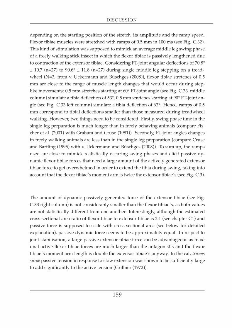
DISCUSSION

depending on the starting position of the stretch, its amplitude and the ramp speed.Flexor tibiae muscles were stretched with ramps of 0.5 mm in 100 ms (see Fig. C.32).This kind of stimulation was supposed to mimick an average middle leg swing phaseof a freely walking stick insect in which the flexor tibiae is passively lengthened dueto contraction of the extensor tibiae. Considering FT-joint angular deflections of 70.8°± 10.7 (n=27) to 90.6° ± 11.8 (n=27) during single middle leg stepping on a tread-wheel (N=3, from v. Uckermann and Büschges (2008)), flexor tibiae stretches of 0.5mm are close to the range of muscle length changes that would occur during step-like movements: 0.5 mm stretches starting at 60° FT-joint angle (see Fig. C.33, middlecolumn) simulate a tibia deflection of 53°, 0.5 mm stretches starting at 90° FT-joint an-gle (see Fig. C.33 left column) simulate a tibia deflection of 63°. Hence, ramps of 0.5mm correspond to tibial deflections smaller than those measured during treadwheelwalking. However, two things need to be considered. Firstly, swing phase time in thesingle-leg preparation is much longer than in freely behaving animals (compare Fis-cher et al. (2001) with Graham and Cruse (1981)). Secondly, FT-joint angles changesin freely walking animals are less than in the single leg preparation (compare Cruseand Bartling (1995) with v. Uckermann and Büschges (2008)). To sum up, the rampsused are close to mimick realistically occuring swing phases and elicit passive dy-namic flexor tibiae forces that need a large amount of the actively generated extensortibiae force to get overwhelmed in order to extend the tibia during swing, taking intoaccount that the flexor tibiae´s moment arm is twice the extensor tibiae´s (see Fig. C.3).

The amount of dynamic passively generated force of the extensor tibiae (see Fig.C.33 right column) is not considerably smaller than the flexor tibiae´s, as both valuesare not statistically different from one another. Interestingly, although the estimatedcross-sectional area ratio of flexor tibiae to extensor tibiae is 2:1 (see chapter C1) andpassive force is supposed to scale with cross-sectional area (see below for detailedexplanation), passive dynamic force seems to be approximately equal. In respect tojoint stabilisation, a large passive extensor tibiae force can be advantageous as max-imal active flexor tibiae forces are much larger than the antagonist´s and the flexortibiae´s moment arm length is double the extensor tibiae´s anyway. In the cat, tricepssurae passive tension in response to slow extension was shown to be sufficiently largeto add significantly to the active tension (Grillner (1972)).

159

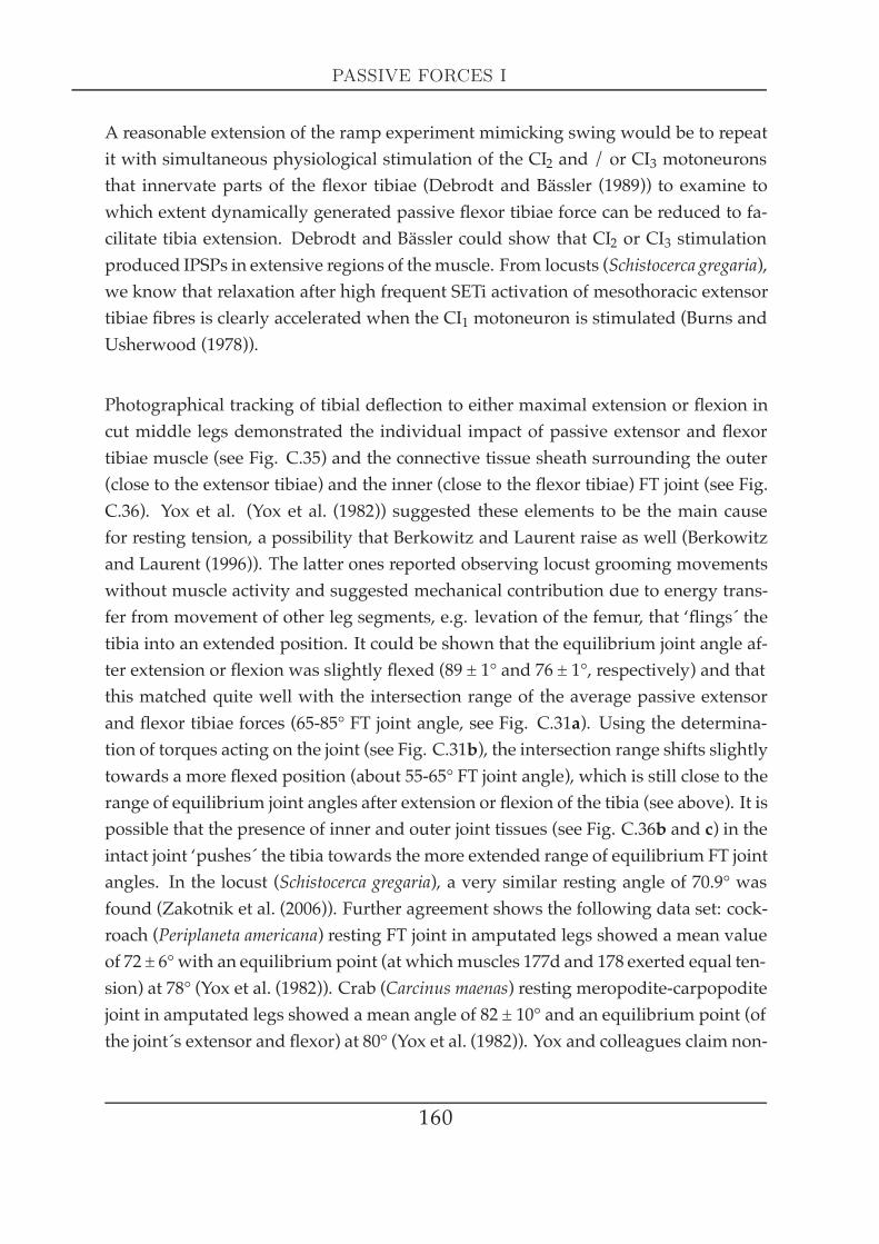
PASSIVE FORCES I

A reasonable extension of the ramp experiment mimicking swing would be to repeatit with simultaneous physiological stimulation of the CI2 and / or CI3 motoneuronsthat innervate parts of the flexor tibiae (Debrodt and Bässler (1989)) to examine towhich extent dynamically generated passive flexor tibiae force can be reduced to fa-cilitate tibia extension. Debrodt and Bässler could show that CI2 or CI3 stimulationproduced IPSPs in extensive regions of themuscle. From locusts (Schistocerca gregaria),we know that relaxation after high frequent SETi activation of mesothoracic extensortibiae fibres is clearly accelerated when the CI1 motoneuron is stimulated (Burns andUsherwood (1978)).

Photographical tracking of tibial deflection to either maximal extension or flexion incut middle legs demonstrated the individual impact of passive extensor and flexortibiae muscle (see Fig. C.35) and the connective tissue sheath surrounding the outer(close to the extensor tibiae) and the inner (close to the flexor tibiae) FT joint (see Fig.C.36). Yox et al. (Yox et al. (1982)) suggested these elements to be the main causefor resting tension, a possibility that Berkowitz and Laurent raise as well (Berkowitzand Laurent (1996)). The latter ones reported observing locust grooming movementswithout muscle activity and suggested mechanical contribution due to energy trans-fer from movement of other leg segments, e.g. levation of the femur, that ‘flings´ thetibia into an extended position. It could be shown that the equilibrium joint angle af-ter extension or flexion was slightly flexed (89 ± 1° and 76 ± 1°, respectively) and thatthis matched quite well with the intersection range of the average passive extensorand flexor tibiae forces (65-85° FT joint angle, see Fig. C.31a). Using the determina-tion of torques acting on the joint (see Fig. C.31b), the intersection range shifts slightlytowards a more flexed position (about 55-65° FT joint angle), which is still close to therange of equilibrium joint angles after extension or flexion of the tibia (see above). It ispossible that the presence of inner and outer joint tissues (see Fig. C.36b and c) in theintact joint ‘pushes´ the tibia towards the more extended range of equilibrium FT jointangles. In the locust (Schistocerca gregaria), a very similar resting angle of 70.9° wasfound (Zakotnik et al. (2006)). Further agreement shows the following data set: cock-roach (Periplaneta americana) resting FT joint in amputated legs showed a mean valueof 72 ± 6°with an equilibrium point (at which muscles 177d and 178 exerted equal ten-sion) at 78° (Yox et al. (1982)). Crab (Carcinus maenas) resting meropodite-carpopoditejoint in amputated legs showed a mean angle of 82 ± 10° and an equilibrium point (ofthe joint´s extensor and flexor) at 80° (Yox et al. (1982)). Yox and colleagues claim non-

160

DISCUSSION

neural resting tension to be used to maintain joint position and further to maintainposture at an energetically low cost in arthropods and found the equilibrium pointresting tension to be approximately equal to the animals weight (Yox et al. (1982)).This is a calculation that may also be true for stick insects like Carausius morosus: withan average mass of 0.94 ± 0.7 g (N=10), an equilibrium point tension of 2.5 - 5 mN iscertainly enough to maintain a gravity independent tibia position: protractor / retra-cor coxae and EMG recordings while rotating the animal in the air in all planes showthat middle leg posture can be maintained throughout with motoneuronal activity be-ing silent (Hooper et al. (2009)). When the animal is hanging in the vertical plane withits longitudinal axis parallel to the ground, the total FT-joint equilibrium point restingtension of all six legs is what is supposed to maintain animal posture, therefore the re-quired resting tension would be F = m · a = 0.94 g · 9.81 ms2 = 9.22mN, i.e. 1.54 mNfor each leg (9.22mN6 ). This calculated value represents a coarse approximation whichis, interestingly, in the same ballpark as the equilibrium point tension is of 2.5 - 5 mN(Fig. C.31). Observing stick insects hanging vertically with their longitudinal axisparallel to the ground reveals that they actually increase the FT-joint angles of all sixlegs (i.e. they extend the tibia compared to standing horizontally): this new joint posi-tion takes advantage of the flexor tibiae static tension characteristic increasing steeperthan the extensor tibiae´s (see Fig. C.31), which might support posture maintainanceof the whole body. It is of special note that ablation of motoneuronal innervation inthe front leg extensor tibiae of Cuniculina impigra can be compensated within 17 daysby shifting the passive static force tension curve towards higher force values: this in-crease in passive tension shifts the FT joint´s equilibrium point towards much moreextended tibia positions (resting positions of 170-180° after 4-16 days, Bässler et al.(2007)). This new equilibrium point enables the animal to use the leg sometimes evenduring walking.

Removal of the connective tissue sheath alone had considerable impact on tibial equi-librium position as well (see Fig. C.36), although tendons of both tibial muscles wereleft intact. Generally, cuticular structures are known to participate in passive forcegeneration in a major way: e.g. locusts (Schistocerca gregaria) can store previouslygenerated large forces in elastic distortions of the tendons and the femoral cuticlerequired for rapid tibia extension (Bennet-Clark (1975); Sasaki and Burrows (2003)).During co-contraction, a locust´s semi-lunar process between femur and tibia is bentprogressively. A cuticular lump is able to lock the FT-joint until extensor tibiae force

161

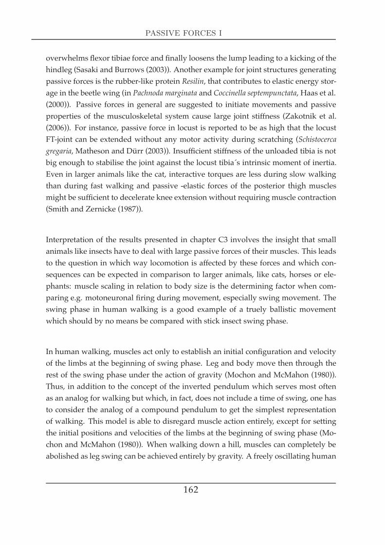
PASSIVE FORCES I

overwhelms flexor tibiae force and finally loosens the lump leading to a kicking of thehindleg (Sasaki and Burrows (2003)). Another example for joint structures generatingpassive forces is the rubber-like protein Resilin, that contributes to elastic energy stor-age in the beetle wing (in Pachnoda marginata and Coccinella septempunctata, Haas et al.(2000)). Passive forces in general are suggested to initiate movements and passiveproperties of the musculoskeletal system cause large joint stiffness (Zakotnik et al.(2006)). For instance, passive force in locust is reported to be as high that the locustFT-joint can be extended without any motor activity during scratching (Schistocercagregaria, Matheson and Dürr (2003)). Insufficient stiffness of the unloaded tibia is notbig enough to stabilise the joint against the locust tibia´s intrinsic moment of inertia.Even in larger animals like the cat, interactive torques are less during slow walkingthan during fast walking and passive -elastic forces of the posterior thigh musclesmight be sufficient to decelerate knee extension without requiring muscle contraction(Smith and Zernicke (1987)).

Interpretation of the results presented in chapter C3 involves the insight that smallanimals like insects have to deal with large passive forces of their muscles. This leadsto the question in which way locomotion is affected by these forces and which con-sequences can be expected in comparison to larger animals, like cats, horses or ele-phants: muscle scaling in relation to body size is the determining factor when com-paring e.g. motoneuronal firing during movement, especially swing movement. Theswing phase in human walking is a good example of a truely ballistic movementwhich should by no means be compared with stick insect swing phase.

In human walking, muscles act only to establish an initial configuration and velocityof the limbs at the beginning of swing phase. Leg and body move then through therest of the swing phase under the action of gravity (Mochon and McMahon (1980)).Thus, in addition to the concept of the inverted pendulum which serves most oftenas an analog for walking but which, in fact, does not include a time of swing, one hasto consider the analog of a compound pendulum to get the simplest representationof walking. This model is able to disregard muscle action entirely, except for settingthe initial positions and velocities of the limbs at the beginning of swing phase (Mo-chon and McMahon (1980)). When walking down a hill, muscles can completely beabolished as leg swing can be achieved entirely by gravity. A freely oscillating human

162

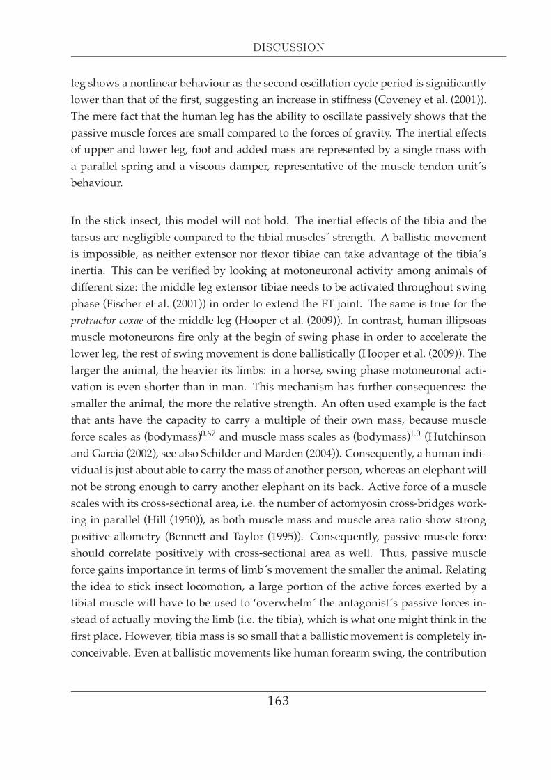
DISCUSSION

leg shows a nonlinear behaviour as the second oscillation cycle period is significantlylower than that of the first, suggesting an increase in stiffness (Coveney et al. (2001)).The mere fact that the human leg has the ability to oscillate passively shows that thepassive muscle forces are small compared to the forces of gravity. The inertial effectsof upper and lower leg, foot and added mass are represented by a single mass witha parallel spring and a viscous damper, representative of the muscle tendon unit´sbehaviour.

In the stick insect, this model will not hold. The inertial effects of the tibia and thetarsus are negligible compared to the tibial muscles´ strength. A ballistic movementis impossible, as neither extensor nor flexor tibiae can take advantage of the tibia´sinertia. This can be verified by looking at motoneuronal activity among animals ofdifferent size: the middle leg extensor tibiae needs to be activated throughout swingphase (Fischer et al. (2001)) in order to extend the FT joint. The same is true for theprotractor coxae of the middle leg (Hooper et al. (2009)). In contrast, human illipsoasmuscle motoneurons fire only at the begin of swing phase in order to accelerate thelower leg, the rest of swing movement is done ballistically (Hooper et al. (2009)). Thelarger the animal, the heavier its limbs: in a horse, swing phase motoneuronal acti-vation is even shorter than in man. This mechanism has further consequences: thesmaller the animal, the more the relative strength. An often used example is the factthat ants have the capacity to carry a multiple of their own mass, because muscleforce scales as (bodymass)0.67 and muscle mass scales as (bodymass)1.0 (Hutchinsonand Garcia (2002), see also Schilder andMarden (2004)). Consequently, a human indi-vidual is just about able to carry the mass of another person, whereas an elephant willnot be strong enough to carry another elephant on its back. Active force of a musclescales with its cross-sectional area, i.e. the number of actomyosin cross-bridges work-ing in parallel (Hill (1950)), as both muscle mass and muscle area ratio show strongpositive allometry (Bennett and Taylor (1995)). Consequently, passive muscle forceshould correlate positively with cross-sectional area as well. Thus, passive muscleforce gains importance in terms of limb´s movement the smaller the animal. Relatingthe idea to stick insect locomotion, a large portion of the active forces exerted by atibial muscle will have to be used to ‘overwhelm´ the antagonist´s passive forces in-stead of actually moving the limb (i.e. the tibia), which is what one might think in thefirst place. However, tibia mass is so small that a ballistic movement is completely in-conceivable. Even at ballistic movements like human forearm swing, the contribution

163

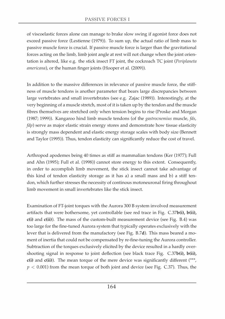
PASSIVE FORCES I

of viscoelastic forces alone can manage to brake slow swing if agonist force does notexceed passive force (Lestienne (1979)). To sum up, the actual ratio of limb mass topassive muscle force is crucial. If passive muscle force is larger than the gravitationalforces acting on the limb, limb joint angle at rest will not change when the joint orien-tation is altered, like e.g. the stick insect FT joint, the cockroach TC joint (Periplanetaamericana), or the human finger joints (Hooper et al. (2009)).

In addition to the massive differences in relevance of passive muscle force, the stiff-ness of muscle tendons is another parameter that bears large discrepancies betweenlarge vertebrates and small invertebrates (see e.g. Zajac (1989)). Interestingly, at thevery beginning of amuscle stretch, most of it is taken up by the tendon and the musclefibres themselves are stretched only when tension begins to rise (Proske and Morgan(1987; 1999)). Kangaroo hind limb muscle tendons (of the gastrocnemius muscle, fds,fdp) serve as major elastic strain energy stores and demonstrate how tissue elasticityis strongly mass dependent and elastic energy storage scales with body size (Bennettand Taylor (1995)). Thus, tendon elasticity can significantly reduce the cost of travel.

Arthropod apodemes being 40 times as stiff as mammalian tendons (Ker (1977); Fulland Ahn (1995); Full et al. (1998)) cannot store energy to this extent. Consequently,in order to accomplish limb movement, the stick insect cannot take advantage ofthis kind of tendon elasticity storage as it has a) a small mass and b) a stiff ten-don, which further stresses the necessity of continousmotoneuronal firing throughoutlimb movement in small invertebrates like the stick insect.

Examination of FT-joint torques with the Aurora 300 B system involved measurementartifacts that were bothersome, yet controllable (see red trace in Fig. C.37b(i), b(ii),c(i) and c(ii)). The mass of the custom-built measurement device (see Fig. B.4) wastoo large for the fine-tuned Aurora system that typically operates exclusively with thelever that is delivered from the manufactory (see Fig. B.7d). This mass beared a mo-ment of inertia that could not be compensated by re-fine-tuning the Aurora controller.Subtraction of the torques exclusively elicited by the device resulted in a hardly over-shooting signal in response to joint deflection (see black trace Fig. C.37b(i), b(ii),c(i) and c(ii)). The mean torque of the mere device was significantly different (***,p < 0.001) from the mean torque of both joint and device (see Fig. C.37). Thus, the

164

DISCUSSION

accuracy of the measurements was impaired, yet the signal resolution was clearly de-tectable.

Torque of the mere FT joint with both extensor and flexor tibiae muscle tendons cutwas shown to be dependent on deflection amplitude (see Fig. C.39) but not on angu-lar position (see Fig. C.38). Physiologically, this has two major consequences. Firstof all, the faster the tibial movement, the more it gets damped as friction is velocitydependent. Secondly, the data show that, within the range of FT angles tested (82° -98°), the force required to deflect the tibia to an equal extent does not increase whenthe tibia is either stretched or flexed, i.e. the joint does not (or only slightly) get stifferwithin a certain range of joint angles. Only a weakly significant (*, p < 0.05) linearincrease could be detected (see Fig. C.38). Thus, the data provides good evidence thatthe FT-joint features the remarkable combination of being position independent andexcursion dependent at the same time.

Such a special arrangement could as well be conceivable for horizontal eye ball move-ments. The muscle-eyeball system is dominated by muscle mechanics, inertia of theglobe makes only minimal effects (Childress and Jones (1967)). However, the muscle-eyeball system is heavily damped. There are other biological examples of having noparticular set point, but being resistant to fast changes: an untrainedmanwalking fastfrom an altitude of 500 m up to 5000 m will get big difficulties with breathing, as theair gets thinner with increasing altitude. In contrast, when doing the whole processstep by step (spending a week at 2000m, another week at 3000 m etc.), the number oferythrocytes will be adapted continously and breathing will be possible even at highaltitudes. Similarly, a person flying from middle Europe to Japan will suffer fromjetlag in the first few nights. After a while, the circadian inner clock operates in thesame way as in Europe, but with an offset of eight or nine hours. The same principlecan also be explained with physical examples: the outer frame of a gyroscope can bepositioned no matter how, it has no preferred position within one degree of freedomwhen the inner wheel is not turning. As soon as the inner wheel is turning, deflectionof the outer rim becomes more difficult, i. e. is has become resistant to fast positionchanges.

165

FORCE MEASUREMENTS IN THE ISOTONIC DOMAIN

D4 Force measurements in the isotonic domain

SummaryIsotonic extensor tibiae experiments in response to physiological motoneuronal in-

put previously gained by recording nerve activity while the animal performed step-like movements suggests the muscle to respond highly variable in terms of the con-traction shapes observed. Nonetheless, response to the same pattern is similar be-tween animals. The muscle acts like a low-pass filter by contracting smoothly to aragged stimulation pattern. Step-like movements arise in most cases from about 40-50 spikes of the FETi motoneuron, mean burst duration is about 0.41 s and meaninterburst interval 2.3 s. Hill hyperbolas at 200 Hz vary much in terms of maximalforce and vary less in terms of contraction velocity for both extensor and flexor tib-iae. Maximally stimulated flexor tibiae muscles are on average 2.7 times strongerthan extensor tibiae muscles (415 mN compared to 151 mN), but only 1.4 times fastercontracting (6.05 mm

s and 4.39 mms ). Both tibial muscles reveal deviations from the

hyperbolic shape close to P0 towards smaller contraction velocities. Isotonic length-ening experiments on the extensor tibiae show this deviation to persist at loads >P0, further loading (> > P0) leads to a sigmoidal curve progression. Extensor tibiaeHill experiments at different stimulation frequencies reveal both V0 and P0 to becomebigger with increased activation. The relation of stimulation frequency with V0 andP0 respectively can be described with an exponential saturation curve of the form

y0 = y0max(1− e− ff0 ), V0 and P0 correlate linearly. The relation between maximal con-

traction velocity and extensor tibiae muscle length can be described with a monotonicand nearly linear increase within the muscle´s working range, followed by a plateauat longer fibre lengths. Velocity of a contraction´s isometric force increase is muchfaster in a muscle being stretched than in relaxed state. Velocity of an isotonic mus-cle length change in turn is only slightly faster in the stretched state compared to themuscle being relaxed. The period in time to increase load to a shortening muscleis crucial: loading the muscle during the first 0.15 s of an isotonic contraction (de-pending on the load) leads to a shortening progression, the same load applied later incontraction leads to a muscle lengthening.

166

DISCUSSION

DiscussionA fourth of the steps analysed in Figs. C.41 to C.43 (22 out of 87) had interburst

intervals > 2 s and were ommitted because of the reasons described above (a robustwalking sequence has a frequency of about 1 Hz). Removal of these step-like move-ments results in a mean interburst interval of 0.77 ± 0.39 s (n=65). With a mean burstduration of 0.41 ± 0.24 s (n=87), step frequency was a little bit less than 1 Hz, which isabout the usual walking speed of adult freewalking Carausius morosus (Bässler (1983)).The discrepancy between the usual swing phase durations of 100-120 ms (Bässler(1983)) and the values measured from these steps might be due to fact that swingphases in tethered animals (single leg preparation, Fischer et al. (2001); Schmidt et al.(2001)) differ a lot in terms of sensory feedback. A tethered, supported stick insectgets different input from the trochanteral and femoral campaniform sensilla, the lat-ters being mainly responsible for the switch from extensor tibiae to flexor tibiae ac-tivity (Akay et al. (2001)). Nonetheless, spike patterns from these steps were usedto drive the extensor tibiae muscle for two reasons: first of all, many stick insect ex-periments over the last years were done with the single leg configuration in animalssupported by a platform (e.g. Akay et al. (2004); Ludwar et al. (2005); Gabriel (2005);Borgmann et al. (2007); v. Uckermann and Büschges (2008)); secondly, there is no rea-son to believe that the actual spiking patterns during single-leg walking are muchdifferent from free walking except for the burst duration, as the animal truely per-forms the actual movement (therefore the extensor tibiae is obviously capable to doit). In general, the motor output has to adapt to changes in the biomechanical prop-erties of the moving parts or to transfer functions of sensory systems, this was testedin several experiments investigating the ability to either adapt or recover, e.g. aftersurgical muscle manipulations (cat: Pearson et al. (1999); Cuniculina impigra: Bässleret al. (2007)). The step sequence presented in chapter C4 is one of seven sequencesanalysed in Hooper et al. (2006; 2007a;b). From these analyses, this sequence doesnot explicitely differ from the other six sequences used. It is essential to know howthe output patterns generated by a representative animal look like in order to designreasonable, physiological relevant stimulation paradigms (nerve stimulation, muscleload, muscle strain) and for the interpretation of the muscle data presented in thisthesis. The knowledge about the actual transformation into movement is of partic-ular importance when analysing brisk motoneuronal output changes, as the musclemight not be able to follow to fast changes anyway. This might seem disadvantageousfor the neuromuscular system at first. However, the extensor tibiae can take advan-

167

FORCE MEASUREMENTS IN THE ISOTONIC DOMAIN

tage of the history-dependent effects described in chapter C2 in terms of producinga smooth movement in response to irregular input. Most of the analysed contrac-tions are typically characterised by a steep increase of instantaneous FETi spikingfrequency (see Fig. C.46 and Hooper et al. (2007a)), which decreases steadily andwhich features long interspike intervals in parts. Due to the initial high-frequent ac-tivation, such gaps could eventually be bridged, as isometric force data in chapterC2 demontrate that relaxation is delayed the more the extensor muscle was activatedbefore (reflected in either more spikes or higher spike frequency, see Figs. C.18 andC.16). Hence, a continuous shortening might be accomplished despite a lack of mo-toneuronal input. This could actually be a common strategy in small insect musclesin locomotion: posterior coxal levator muscles 182C and 182D in the cockroach Peri-planeta americana show maximum frequency of the coxal depressor motoneuron D8 tooccur at the burst beginning as well (Pearson and Iles (1970)). In contrast, vertebratemuscle is likely to respond much faster (Edman (2005); Lappin et al. (2006)), i.e. therequirement of a persistent firing pattern is bigger in order to shorten smoothly, be-cause large interspike intervals would immediately be transformed into a relaxation.

As described by Hooper and colleagues (Hooper et al. (2006)), stepping behaviourcan be very different in terms of contraction shape, i.e. the muscle length changesthat are finally move the limb. As was shown in chapter C4, the muscle shorten-ings can either have a rather trapezoidal or a rather triangular shape, they can eitherhave a multi-sloped shortening phase or a multi-sloped relaxation phase. By manyparameters (e.g. slope of the contraction rise or fall), extensor tibiae muscles from dif-ferent individuals differ statistically from one another (detailed quantitative analysisin Hooper et al. (2006)). Overdrawn contractions allow the impression that extensortibiae muscles of five examplary animals respond similarly to the same physiologicalinput at first sight (Fig. C.44). Having been subject to further more detailed analy-sis, extensor tibiae muscles responded indeed similarly to changes in neural input, atleast on a burst-to-burst level (Hooper et al. (2006)). When contractions are plottedversus spike number, and not time, the rises per spike were identical (Hooper et al.(2007b)), which could already be shown for the lobster (Panulirus interruptus, Morrisand Hooper (1997)). Hence, extensor tibiae muscles present a single population, eventhough there is considerable animal-to-animal variation. This is a very importantfinding as this enables averaging muscle data across animals (Hooper et al. (2006)),which was performed throughout this thesis. Driving the muscle with previously

168

DISCUSSION

recorded FETi motoneuron patterns recorded during step-like movement activity issupposed to mimick a physiological situation quite close. Although FETi, SETi andCI1 are simultaneously active during middle leg swing (Büschges et al. (1994)), theSETi motoneuron´s main role is most likely to maintain posture. In the locust middleleg, tension rise time in response to SETi stimulation is nearly 1 sec and cannot be themain determinant in walking (Schistocerca gregaria, Burns and Usherwood (1978)), al-though SETi is active with FETi being silent at the beginning of retraction (Burns andUsherwood (1979)). In the locust hind leg, SETi is the only excitatory extensor mo-toneuron to be active during walking (Burns and Usherwood (1979)). Physiologicalstimulation of the SETi motoneuron (previously recorded during walking and thenplayed back) results in very smooth isometric force generation (Schistocerca gregaria,Evans and Siegler (1982)). This smoothness is very likely to be the consequence ofthe SETi´s low fusion frequency (Burns and Usherwood (1978)). Similarly, isometriccockroach force traces of posterior coxal levator muscles 182C and 182D shown byPearson and Iles (Periplaneta americana, Pearson and Iles (1970)) reveal these musclesto respond very slowly as well. Thus, the extensor tibiae is one among several in-vertebrate muscles that acts like a low-pass filter as it shows smooth contractions inresponse to rather ragged input (see Figs. C.44, C.45, C.46, C.47), comparing instan-taneous frequency traces with muscle position traces (see Fig. C.46). Different fromprevious work, the extensor tibiae measurements were done in the isotonic force do-main.

In order to reveal the extensor and flexor tibiae´s force-velocity characteristic (Hillcurve, Hill (1938)), a series of loaded release experiments was conducted with tonicinput of different frequency. In contrast to the experiments with physiological stimu-lation, Hill experiments require tetanical stimulation before application of a clampedload level. The force-velocity curve can be considered as one of the many output char-acteristics of an underlying contraction principle (Ettema and Meijer (2000)). This isa major distinction from the length-tension curve, which is explained by structuralmodels, e.g. the crossbridge theory (Huxley (1957a); Ettema and Meijer (2000)). Im-mediately after the transition from isometric to isotonic mode recording, contractionoscillations occurred (Jewell and Wilkie (1958); Edman (1988); Malamud and Joseph-son (1991); Edman and Curtin (2001); Siebert and Blickhan (2003)). Those may reflectthe fast dynamic properties of the contractile mechanism under fast length change.Jewell and Wilkie explained those oscillations with the elastic properties of the series

169

FORCE MEASUREMENTS IN THE ISOTONIC DOMAIN

elastic element represented by one of the springs in Hill´s three component model(Hill (1938)). According to Podolsky and Nolan, an isotonic step change runs throughdifferent phases: between the original steady state with a certain distribution of at-tached cross-bridges and the final steady state featuring a different distribution ofcross-bridges, there is a transitional state of zero-distortion, showing a distributionof negative distorted cross-bridges that equals the distribution of positively distortedones. This ‘gap´ is the reason for the system´s oscillatory response aided by the steepincrease in stiffness of attached cross-bridges in the region of negative distorted cross-bridges (Podolsky and Nolan (1972)). Edman described the oscillatory course as a‘recoil of elastic structures, being situated in the inner sarcomere´ (Edman (1988)).Oscillations in frog muscle fibres can have durations > 80 ms (Civan and Podolsky(1966); Sugi and Tsuchiya (1981)). Edman mentions experiments showing oscillationsthat persisted during the whole duration of load clamp, when the applied load wasabout 0.9 P0 (Armstrong et al. (1966); Edman (1988)). Extensor tibiae oscillations haddurations from about 17 to 25 ms, depending on stimulation frequency. Isotonic ex-tensor tibiae experiments being discarded because of the whole measuring systemhaving been not stiff enough (the hooked-shaped insect pin pierced through the mus-cle tendon was attached to the servo motor via a silk filament and the mounting ofthe servo motor was more compliant) had durations from about 50-60 ms (N=3, datanot shown). After these oscillations, initial contraction velocity which declines ratherrapidly to zero is the result of the short fibre length and of the force-length character-istics of the extensor tibiae: by shortening, the muscle moves to a shorter length withreduced maximum force which results in a reduced contraction velocity. The contrac-tion stops at the muscle length at which the maximum isometric force is equal to theload set in the experiment (see Fig. C.49. Thus, measuring the contraction velocity ofa muscle yields automatically in getting active force - length data as well. This ‘side-effect´ was ignored within this thesis, but not in the data evaluation for the musclemodel (Blümel et al. (2007a;b; 2008b;a)).

Extensor tibiae force-velocity curves show the well known hyperbolic shape of theHill-curve, for which there are basically two main explanations. Firstly, the meanforce that a single cross-bridge exerts decreases with increasing shortening velocity.This can be traced back to the fact that negatively distorted cross-bridges exert lessforce than positively distorted ones (see Huxley (1957a)). Secondly, the mean numberof attached cross-bridges per time unit decreases with increasing shortening velocityas well. This can be traced back to the fact that negatively distorted cross-bridges are

170

DISCUSSION

more likely to detach than positively distorted ones (see Huxley (1957a)). Hill-curvemeasurements produced maximum isometric contraction forces that varied between90 mN and 200 mN at activation of 200 Hz (see Fig. C.50 and Tab. C.7). The rangeof maximum contraction velocities was much narrower: 3.6 mms to 4.8 mms . In respectto effective cross-sectional area (1.91 mm2), tensions were 4.8 to 10.5 N

cm2̂. In respect

to fibre length (1.41 mm), contraction velocities ranged from 2.6 to 3.4 FLs . Althoughabsolute maximum isometric forces and contraction velocities were shown to differ alot between extensor and flexor tibiae (compare Fig. C.50 and Tab. C.7 with Fig. C.51and Tab. C.8), more detailed analysis of the data provides evidence that the musclesare not that different:

Similar to the extensor tibiae, the variation of maximum isometric flexor tibiae forcesat 200 Hz was also much larger than the variation of maximum shortening veloci-ties (see Fig. C.8). This result is hard to interpret because neither the measurementmethod should lead to more variability of one parameter compared to the other norshould differences in molecular processes (e.g. cross-bridge cycling) be responsiblefor such a discrepancy. Mean maximum flexor tibiae forces were more than two anda half times as large as extensor tibiae forces (see chapter D2). However, mean maxi-mal flexor tibiae contraction velocities were only 1.4 larger than those of the extensortibiae. Related to cross-sectional area and mean fibre length (4 mm2 and 2.11 mm,see chapter C1), determined flexor tibiae tensions and velocities are very close to theones determined for the extensor tibiae (determined using 1.94 mm2 and 1.41 mm,see chapter C1). When normalised to fibre length, relative maximum velocities are2.87 ± 0.43 Fl

s for the flexor tibiae compared to 3.12Fls for the extensor tibiae, when

stimulated maximally. These values are rather at the lower end of the spectrum ofdata known for different muscles, indicating stick insect leg muscles are adapted togenerate slow movements. In a similar range are mouse fibres from the hindlimbflexor digitorum brevis muscle (4.0 ± 0.3 Fl

s , Edman (2005)), frog fibres from the ante-rior tibialismuscle (2.01 ± 0.05 Fl

s , Edman (1988)). Clearly faster contracting are fibresfrom the Tcx2 muscle in Schistocerca americana (5.2 ± 0.1 Fl

s , Malamud and Josephson(1991)), from cockroach extensors 177c and 179 (Blaberus discoidalis, 5.7 ± 0.4 Fl

s and 4.9± 0.4 Fl

s , Ahn and Full (2002)), the cat soleusmuscle (4.82Fls , Spector et al. (1980)) and

skeletal muscles of the frog (8.2 ± 1.9 Fls , Edman (2005)). Much faster contracting are

tentacle fibres from the squid Loligo paleiwith a maximum contraction velocity of 15.4± 1.0 Fl

s (Kier and Curtin (2002)) and fibres from the cat medial gastrocnemius muscle

171

FORCE MEASUREMENTS IN THE ISOTONIC DOMAIN

(12.87 Fls , Spector et al. (1980)).

As already discussed in chapter D1, the comparison between extensor and flexor tib-iae shows further similarities in respect to their maximum shortening velocities andthe numbers of sarcomeres determined for the extensor tibiae (∼ 200) and for theflexor tibiae∼ 300). Contraction velocity depends on sarcomere number (Huxley andNiedergerke (1954b); Thuma (2007); Thuma et al. (2007)) and the flexor tibiae having1.5 times more sarcomeres than the extensor tibiae predicts therefore that the flexortibiae shortens 1.5 times faster maximally than the extensor tibiae, which it almostdoes: V0 = 6.05 mm

s for the flexor tibiae (N=8) and V0 = 4.39 mms for the extensor tib-

iae (N=7), see Tabs. C.8 and C.7). An asymmetry of maximum shortening velocitiesin antagonistic muscles is not unusual: in the ghostcrab Ocypode quadrata, the extensorcarpopodite has a V0 of 4.6 - 4.7 Fls and the flexor carpopodite has a V0 of 5.6 - 7.0

Fls (Perry

et al. (2009)).

Measurements of contraction velocity at altered load levels > P0 (i.e. stretch) can bedescribed as being eccentric (the muscle is lengthened while being active), see Figs.C.52 and C.53. Muscle soreness is a painful experience that probably everyone mighthave experienced and which is known to be the consequence of eccentric exercise(Whitehead et al. (2003)). One might assume that such eccentric exercise occurs to alarge amount when walking downhill (‘when muscles have to absorb the momentumof the body during jumping and running´, Edman et al. (1997)), which is supposedlymore energy-consuming than going uphill. The theory behind this proposition com-prises the occurence of disrupted sarcomeres in series with still-functioning sarcom-eres increasing series compliance and therefore reducing passive tension and shiftingthe optimum length for peak active force (toad sartorius muscle, Wood et al. (1993);amphibians and humans, Jones et al. (1997); humans, Whitehead et al. (1998)). Inaddition, factors such as metabolic exhaustion, structural filamental damage or elec-tromechanical coupling failures contribute to a reduction in actively generated force(reviews by Morgan and Allen (1999); Proske and Morgan (2001)). With respect tothe eccentric experiments presented in this thesis, care was therefore taken to stop theexperiment when muscle rundown was obvious in terms of P0reduction exceeding15%. Loads were therefore gradually increased until measurable muscle damage wasappearing. Permanent after-effects indicating a weakening or complete break of some

172

DISCUSSION

contractile links were regularly found after application of several rapid stretches (sar-torius muscles of Rana temporaria and Rana esculenta, Katz (1939)). Direct in vivo ten-don force and indirect ground reaction force measurements on the ankle extensorsof the kangaroo rat showed that a range of 45 to 175 % of the in situ measured iso-metric peak force are utilized by the animal during locomotion. The way the animaljumps involves rapid stretching of the muscles while being active (i.e. eccentric ex-ercise), which comprises operations on the lengthening region of the force-velocitycurve (Katz (1939); Biewener et al. (1988)). This is a good example of how force levels> P0 are actually used and how they can become essential for the capacity of an an-imal´s locomotory possibilities. The ankle joint dynamics of the cat paw-shake cycleare another good example for such eccentric exercise: active forces are derived pri-marily from lengthening contractions, assuring e.g. that extensor activity coincideswith the development of peak extensor torque and the slowing of knee flexion (Smithand Zernicke (1987)).

Previous reports have shown that the Hill-curve deviates from a hyperbola when con-traction velocity is very small andmuscle force is close to beingmaximal (Edman et al.(1976) Edman et al. (1978) above force values of 0.65 P0, the corresponding velocityvalues are markedly lower than those predicted by the hyperbolic fit and that datafrom eccentric experiments cross the abscissa (zero velocity) with a slope near zero(Edman et al. (1976; 1978)) for single muscle fibres, the curve can be seen to be flat(Edman (1988)). Edman explains the deviations in the high force range as a reducedcontraction velocity. In accordance to the findings in this thesis (Figs. C.52 and C.53),he sees no discontinuity in the force-velocity relation around P0 (i.e. forces < P0 and> P0), as seen by e.g. Katz: a consistent divergence between the observed and calcu-lated speed of isotonic lengthening; the actual velocities being several times smallerthan the theoretical (Katz (1939)). There are two conceivable mechanisms that couldbe taken as a basis for the ‘double-hyperbolic´ shape of the Hill curve.

One explanation comprises the possibility that the deviation may result from an in-trinsic Coulomb-friction in the muscle fibres. This would result in a reduced activecontraction force and would lead to the sigmoid zero crossing of the Hill curve whenchanging the direction of movement. The consequence of this intrinsic friction wouldbe that high passive forces would need to be overcome before movement could oc-

173

FORCE MEASUREMENTS IN THE ISOTONIC DOMAIN

cur. Physiologically, this could be the case when the load affecting tibia movementchanges, e.g. at the transition from swing to stance in walking of the stick insect mid-dle leg (Karg et al. (1991); Bässler (1993a); Büschges (1995b); Fischer et al. (2001)).

Another explanation concerns cross-bridge cycling. Edman and colleagues describe akind of a ‘highly effective intracellular servomechanism´ that is of particular signifi-cance in situations when the muscle is suddenly overloaded and claim that an extra-muscular mechanism could hardly provide an equal protection from overstretch (Ed-man et al. (1997)): that is, the biphasic shape of the force-velocity curve can promotemechanical stability. They claim cross-bridges in striated muscle to act as indepen-dent force generators under various loading conditions of the muscle. The averageforce per cross-bridge is then reflected by the force/stiffness ratio. They further claimforce output per bridge to be lower in the high-force range than expected from mea-surements at low and intermediate loads and suggest a model that can be alignedwith the classical crossbridge works from Huxley (Huxley (1957a)) and Huxley andSimmons (Huxley and Simmons (1971)): force during shortening is a function of across-bridge´s attachment rate constant, its traverse distance during a working strokeand its detachment rate constant. Force is assumed to be generated in several steps,where each step leads to a tighter binding between actin and myosin and therefore toa greater force production (Huxley and Simmons (1971); Eisenberg et al. (1980)). Thisbinding sequence comprises three states of cross-bridge attachment during a work-ing cycle (the powerstroke), the first two occuring proportionally more often duringisometric conditions and during shortening at low velocity and the last one, being thestrongest bound, mostly occuring during shortening (Lombardi and Piazzesi (1990);Piazzesi et al. (1992); Edman et al. (1997)). The beginning of the powerstroke fea-tures a region of slow cross-bridge attachment leading to a marked decrease in thenumber of attached cross-bridges and in further consequence to a fairly large dropin force (which can be measured in the Hill´s curve flat region around P0). This isthe direct conclusion from the assumption that the attachment rate constant in themodel by Edman and co-workers shows a Gaussian distribution in respect to thecross-bridge position (Edman et al. (1997)). Huxley (Huxley (1957a)) suggested thatthe force exerted by an attached bridge might be proportional to its distortion andthat the probability for an attachment might be higher at positive crossbridge distor-tions. On the other hand, detachment might occur more often when filament slidinginduces cross-bridges to attain small distortions and therefore to exert little forces.The higher the contraction velocity, the greater the proportion of cross-bridges hav-

174

DISCUSSION

ing negative distortions and resisting the shortening. The total amount of attachedcross-bridges decreases. At maximum shortening velocity, forces from bridges withnegative distortions equal the forces from bridges with positive distortions.

Looking at forces occuring in reponse to muscle lengthening, the increase to forces >P0 can be explained again in terms of cross-bridge cycling. During lengthening, thenumber of crossbridges would be less than during isometric (increased probability ofbreakdown), but individual links would exert a larger force (Joyce et al. (1969)), justlike springs would. If this extra force of individual links outweighed the reductionin their number, the tension during lengthening would exceed the isometric tension.The most strained (or distorted) bridges are the least stable ones and thus the firstones to break (Cavagna and Citterio (1974)).

While the length dependence of contraction force was a direct indication for the dif-ferent degree of thick and thin filament overlap (Gordon et al. (1966b)), the questionof whether the contraction velocity also depends upon fibre length is not as straightforward. White treated the contraction velocity according to Gordon et al. (1966b) asbeing independent of fibre length and coined the ‘tug-of-war-concept´: “The tensionsuch a team can exert is proportional to the number of members in that team, but if therope between two teams is cut, then the maximum rate at which the team can moveis the speed with which any individual member can run (White (1977)).” However, indoing so, White cited Gordon et al. (Gordon et al. (1966b)) incompletely: Gordon etal. stated for long fibre lengths beyond the resting length that V0 changes only little(15%) with length, while isometric force P0 declines from 100% to 40%. The data inchapter C4 show a similar broad plateau, much broader than the narrow maximumof the force-length curves presented in chapter C2 (compare Fig. C.56 with Figs. C.23and C.24). But Gordon et al. show explicitly that for shorter fibre lengths the maxi-mum contraction velocity V0 decreases linearly with fibre length, in agreement withour findings. Abbot and colleagues (Abbot andWilkie (1953)) also show this for shortfibre lengths. Edman Edman (1979) finds a similar result for short fibre lengths, but anincreased V0 in the range of long fibre lengths, presumably caused by the increasedresting tension of the fibres. Although it was not possible to measure the contractionvelocity without any load with the experimental design used within this thesis, theresidual load was attempted to be kept as small as possible. The residual load at 200

175

FORCE MEASUREMENTS IN THE ISOTONIC DOMAIN

Hz accounts for 1% (filled circles) and 3% (open circles) of the maximum contractionforce P0 (the values of the rest load are not shown). Under these conditions, the con-traction velocity decreases to 50% at short fibre lengths, whereby the relative loadincreases to 1.6% (5%) because of the decreasing maximum contraction force. The mi-nor rise in relative load is negligible, the length dependence is for real: it is highlyimprobable that the effect shown will turn into a completely different characteristicjust because of this marginal increase.

The 50 Hz curve shows that an increase in relative load can indeed falsify the lengthdependence: here, the relative portion increases from 2% to 80% of the maximum con-traction force. The contraction velocity falls back to almost zero, because the stronglyreduced contraction force at this length has almost reached the force value of the resid-ual load.

Especially in terms of aiming for muscle modelling, a very essential investigationconcerned the dependence of the extensor tibiae Hill-curves across a range of stim-ulation frequencies that covered the physiological firing range (30-200 Hz) of the ex-tensor motoneurons (see Fig. C.54 and Tab. C.9). Both maximum contraction force(P0) and maximum contraction velocity (V0) greatly increased with frequencies up toaround 60 Hz and then began to level off, achieving near maximum values at fre-quency values beyond 100 Hz (see Fig. C.55a and b). This is consistent with the factthat contraction amplitude at large spike numbers does not increase in tonic stimu-lations at spike frequencies > 100 Hz, although spike frequencies up to 325 Hz canoccur in real physiological bursts (see e.g. v. Uckermann and Büschges (2008)). Assuch bursts are usually highly variable, variation in average spike frequency above100 Hz can still have functional effects (Hooper et al. (2007b)). The curvature of theHill-characteristics is greater at low activation compared to higher activation (see ‘c´ -values for Fig. C.54 and Tab. C.9). Similar observations were made in the frog, whereF-V curves were measured during different times after tetanus onset (13% P0, 25%P0 and 100% P0) and curvature was greater at lower activation, i.e. early in tetanus(Edman and Josephson (2007)).

Both P0 and V0 data sets were well fit with equations of the form P = P0max(1− e− ff0 )

and V = V0max(1− e− ff0 ) in which the mean ‘frequency constants´ f0 were identical

176

DISCUSSION

(see Fig. C.55a and b). f0 may reflect the time constant of a process common to bothforce production and contraction velocity such as Ca2+-summation. Consistent withthis common dependence, V0 and P0 were linearly correlated with each other in sin-gle preparations, although some animal to animal variability was present (see Fig.C.55c). Summarising, these data suggest that for the control of force and contractionvelocity of the extensor tibiae, changes in motoneuron firing are most effective be-low 80 Hz. The differences between P0 and V0 at 80 Hz and 200 Hz activation aremuch less than between 30 Hz and 80 Hz activation. In great similarity with theseobservations, activation-frequency relationships of the caudofemoralis muscle in thecat show that differences in activation are strongest between 20 and 60 Hz (Brownet al. (1999)). Another examination on human wrist flexors demonstrates as well thatmaximum shortening velocity of muscle should be scaled with activation, 20-100%P0 at intervals of 20%: P0 and V0 show an almost linear relationship (‘best fit´, Chowand Darling (1999)). The main interest of this particular set of experiments was toassess frequency-dependence of V0 and P0 and not to additionally look for the lengthdependence of this curve as Brown et al. (1999) or howmaximum contraction velocitycould be assessed using much higher stimulation frequencies (up to 400 Hz, De Haan(1998)). Rack and Westbury fitted their isometric muscle data similarly, except fordescribing the whole stimulation frequency - tension relation with a sigmoidal ratherthan an exponential function, as P0 wasmaximal at 50 Hz (Rack andWestbury (1969)),instead of 200 Hz for the extensor tibiae. P0 between 1 and 10 Hz seems to increaseless than between 10 Hz and 20 Hz for the cat soleusmuscle. As this range of stimula-tion frequencies was not tested for the extensor tibiae, it is hard to tell if a sigmoidalfit would have been the most reasonable fit for the extensor tibiae as well. Noticeably,the stick insect computer muscle model does operate with a sigmoidal fit, as singletwitch data points (1 Hz) are included (Blümel et al. (2007a;b; 2008b;a)).

Similar to the parallel length dependence of V0 and P0 at shorter fibre lengths, the dataprovided shows that there is also an approximately parallel influence of excitation onV0 and P0 (Fig. C.55c). Experiments of Malamud and Josephson on the locust and ofJewell andWilkie on the frog, where force-velocity curves were measured at differenttimes during a single twitch provide suitable results: both V0 and P0 change similarlywith excitation (Tcx2 flight muscles in Schistocerca americana, Malamud and Josephson(1991); sartorius muscle in Rana temporaria, Jewell and Wilkie (1960)). Similar to vari-ation of motoneuronal stimulation frequency, different times during a single twitch

177

FORCE MEASUREMENTS IN THE ISOTONIC DOMAIN

represent different ‘degrees of activation´ (see Malamud and Josephson (1991)), refer-ring to the term ‘active state´ (Hill (1938)). The ‘active state force´ is the force whichthe contractile component of a muscle could just maintain without shortening or be-ing lengthened (Hill (1949); Edman (1970); Edman and Kiessling (1971); Malamudand Josephson (1991); Edman and Josephson (2007)).

The variablility of the data, especially of P0- values is an issue that demands furtherinterpretation. Maximum tetanical extensor tibiae force at 200 Hz has a S.D. of ±29.8% (see Tab. C.7), single twitch force varies even more (S.D. of ± 94%, see Tab. C.3)and maximum extensor tibiae contraction velocities feature a S.D. of ± 9.1%. For theflexor tibiae, a similar variability arises: at maximal recruitment, tetanical force at 200Hz shows a S.D of ± 30% and maximum contraction velocities have a S.D. of 15%. Insearch of parameters that might justify these large variations, a set of ten extra animals(representative for animals used in all examinations within this thesis) weremeasuredin size and mass and demonstrated mean body length to be L=77.1 ± 2.28 mm andmean body mass to be M=940±70 mg (seeMaterials and Methods section). From theseminor inter-animal variations (S.D.s of ± 3% and 7%, respectively), it is hard to reasonthe discrepancies measured. There are two arguments that a systematic preparationerror is rather unlikely. First, within sets of experiments, the magnitude of variationis not the same for different parameters: for both tibial muscles, maximum contrac-tion velocity varies much less than maximum tetanical force. Second, in differentsets of experiments, a large variation can be found as well: determination of extensorand flexor tibiae fibre lengths, extensor tibiae relaxation time constants after differ-ent activation, the extensor tibiae force-length characteristics, flexor and extensor tib-iae dynamic passive forces, extensor tibiae contractions in response to physiologicalinput and extensor and flexor tibiae quick-release experiments including determina-tions of P0, V0 and the spring constant β. The magnitude between different sets iscomparable, e.g. Tabs. C.7 and C.8 , Figs. C.62 and C.60 or Fig. C.55. This large de-gree of variation is apparently a property of the extensor tibiae (Hooper et al. (2006);Guschlbauer et al. (2007); Hooper et al. (2007a;b)) and seems to apply for the flexortibiae as well, other stick insect leg muscles are not yet examined. In the flexor tibiae,it could be argued that variation in P0 or V0 could arise from different levels of recruit-ment. As described in the ‘Materials and Methods´ section, stimulation current was setto an amplitude where further increase did not result in a further isometrical forceincrease. Hence, it was assumed that this current level was eliciting action potentials

178

DISCUSSION

in all flexor motoneurons, yet a test recording from the ncr nerve was not consideredbecause of the high number of motoneurons (e.g. Goldammer et al. (2007)). As thedegree of flexor tibiae force and contraction velocity variablity was not higher thanthe extensor tibiae´s, different levels of recruitment are apparently not the source ofvariability.

A very essential revelation is the finding that other insect leg muscles show consid-erable variability in contraction force as well, for example the extensor 117c in thecockroach (Blaberus discoidalis, Ahn and Full (2002)) or pro- andmesothoracic extensortibiae in Schistocerca gregaria (Burns and Usherwood (1978)): relative standard devia-tions of force in the cockroach at twitch ± 38 %, at tetanus ± 31%, and in the locust attwitch ± 30% in response to prothoracic and ± 48% in response to mesothoracic FETistimulation. These specifications are in a similar range as some of the extensor tibiaeforces measured in this thesis (± 72.3% at twitch, ± 47.9% at 50 Hz stimulation and ±29.8% at 200 Hz stimulation (see C.6). In vertebrate muscles, high variability can bealso found: passive force of the cat soleusmuscle at optimal fascicle length had a S.D.of 120% (Scott et al. (1996)).

Investigating the kinetics of isometric force development and isotonic shortening atdifferent muscle lengths (see Fig. C.57) led to several interesting insights. Extensortibiae shortening verlocities at 50 Hz against a small load were within the same rangethat might be expected from C.54: about 3 mm

s (see Fig. C.57a(ii)). From the lengthdependence of maximum shortening velocity (see Fig. C.56), one might expect themuscle starting at higher stretch to shorten faster. As the load applied was chosento be equal to the passive force at the respective length, the slightly increased loadobviously ‘compensated´ for the higher stretch and led to approximately the sameshortening velocity. Edman and Josephson (Edman and Josephson (2007)) measuredHill curves in Rana temporaria at different times during isometric contraction rise andrevealed V0 to remain approximately the same and detected only a shift along theforce axis. Interestingly, isometric contraction at larger stretch results in much largervelocity of force increase than at less stretch (see Fig. C.57a(i)). Using maximumvelocity as a ‘degree of activation´ (see Hill (1949); Malamud and Josephson (1991)to this topic) , activation is complete by the time that isometric force has risen to aquarter of its plateau value. This is faster than expected by the isotonic and isove-

179

FORCE MEASUREMENTS IN THE ISOTONIC DOMAIN

locity experiments of Edman and Josephson, they claim activation to be complete byapproximately half the plateau value (Edman and Josephson (2007)). The cause forthe higher force rise velocity at larger stretch could be the series elastic component,as an increase in stiffness leads to a faster gain of force per time unit. The fact, thatthe ratios of isometric forces and isotonic shortening amplitudes musclestretchedmusclerelaxed are verysimilar is a logical consequence of the force-length relationship: the muscle shortensby ‘descending´ the ascending leg of the force-length curve.

It was demonstrated that the time of externally applied forces during muscle contrac-tion is crucial, especially in respect to the direction of a limb´s movement. As couldbe shown in chapter C4, loading the extensor tibiae 0.12 s after the begin of an iso-tonic shortening will lead to a further shortening, whereas the same amount of loadbeing applied after about 1 s of shortening will lead to a sudden lengthening (see Fig.C.58b). Dean could show that load changes are met with rapid adjustments (often< 20 ms; Dean (1984)). He measured stick insect protraction speeds in the presenceof increased loads (up to 0.75 g, i.e. ca. 7.5 mN applied to the tibia) and concludedfrom the fact that protraction continued in spite of the opposing forces the occurenceof a motor output enhancement. Protraction speed was not maintained. Similarly, inlocusts a high-gain position control loop is assumed to be responsible for load com-pensation (Matheson and Dürr (2003)). In general, muscles are thought to respondto perturbations by way of active neural reflexes. However, such more immediateresponses can result from the muscle´s intrinsic force-length and force-velocity prop-erties (Rack (1970); Grillner (1972); Jindrich and Full (2002); Blickhan et al. (2003)) andwere termed ‘Preflexes´ (Full and Koditschek (1999); Brown and Loeb (2000a)). Inaddition to such preflexes, there is the possibility that the morphology (leg geome-try and skeleton properties) represents a mechanical feedback controller (Kubow andFull (1999)). Passive muscle properties can act qualitatively like a negative positionfeedback system (Polit and Bizzi (1978); Hogan (1982); Bartling and Schmitz (2000)) orcan contribute to joint impedance in a stabilising way together with the connective tis-sue (Brown et al. (1982); Esteki andMansour (1996); Hajian and Howe (1997); Jindrichand Full (2002)). Muscle properties constitute a peripheral feedback system that hasthe advantage of zero time delay. When perturbations during a movement paradigmare not too large, e.g. human vertical jumping, the task might be performed suc-cesfully without any necessity of adapting the muscle stimulation pattern (van Soestand Bobbert (1993)). Movement does not need to be actively controlled to exhibit

180

DISCUSSION

dynamic stability (Jindrich and Full (2002)). Even in vertebrate muscles (e.g. in thecat), which are in general faster responding than invertebrate ones, only muscle stiff-ness can provide a load compensation, because the delays between a change in motorunit discharge and tension development are too long to allow a reflexly induced loadcompensation during e.g. gallop (Grillner (1972)). In two experiments (examplaryfigure of the principle mechanism given in chapter C4), investigations aimed to testhow large a load increase during contraction had to be to cease the actual shorteningprocedure. Fig. D.2 shows that loads up to > 30 mN applied 0.12 s after contractionstart do not prevent the extensor tibiae muscle from continuing to shorten.

The experimental paradigm used (Figs. C.58 and D.2) was designed to be close toDean´s, who applied loads opposing protracor coxae contraction directly on the hindleg, 0.1 to 0.2 s after protraction begin (from what could be estimated from the figurein the paper). Although loads were applied directly on the tendon (and not on the leg)and themuscle in focus was the extensor tibiae (and not the protractor coxae), the dataprovided in this thesis suggest the persistence of the protraction movement recordedby Dean to be rather a muscle property than a positive feedback reflex mechanism(as claimed by Dean (1984)). This suggests a new approach to the term of preflex be-haviour: the middle leg extensor tibiae (or any ‘slow contracting´ muscle) can takeadvantage from its slowness and from the fact that it will only rarely reach a steady

Figure D.2: Extensor tibiae shortening amplitudes after various load increases from two experiments(N=2, n=7). Load increase was applied 0.12 s after isotonic contraction begin. The linear regression fit(solid line) is highly significant (< 0.001, ***, R=-0.987).

181

PASSIVE FORCES II

contraction state within a physiological situation like a fast swing phase consisting ofabout 40 FETi spikes (see chapter C4 and Hooper et al. (2007a)). Fig. C.11 and Tab.C.5 show the kinetics at different activation levels. As described earlier in respect toquick release experiments, the muscle ‘weakens itself´ by shortening and the contrac-tion reaches a steady state when the applied load equals the force the muscle can exertat a particular length: it descends along the ascending leg of its force-length charac-teristic. Thus, the slowness of shortening development enables the muscle to resistloads for a longer period of time. As long as the load is not too large, the muscle willtherefore nearly always continue to shorten when being perturbed. In contrast, frogskeletal muscle fibres (Rana temporaria) are much faster contracting: they need 59 ± 4ms to reach 90 % of maximum tetanic force (Edman (2005)). This has dramatic con-sequences in respect to the preflex mechanism because a sudden perturbation > 0.06s after contraction begin would lead to a fibre lengthening and the above described‘zero delay peripheral feedback system´ (van Soest and Bobbert (1993)) would fail orrather would not exist. This effect is mimicked by stick insect loading experimentswith load increases after nearly 1 s (see Fig. C.58b), that show that a perturbationleads to a fibre lengthening as the muscle is about to reach a steady state and is con-sequently weaker than before because of the force-length characteristic. Thus the par-ticular time point of disturbance occurence is crucial: whether the muscle is in therising phase of an isotonic contraction or whether it has reached a constant lengthlevel. To the author´s knowledge, the currently suggested mechanisms describing thepreflex behaviour do not yet consider that slow muscle kinetics are essential in orderto benefit from the stabilising effect of the force-length characteristic.

D5 Passive forces II

SummaryQuick release experiments provide not only contraction velocity data (see chapter

C4), but reveal also the properties of the muscle´s series elastic component. It turnsout that extensor and flexor tibiae series elasticities act like nonlinear springs, data-points measured at a particular stimulation frequency can be fitted with a parabola:the muscle gains stiffness with increasing force. By shifting individual parabolas rep-resenting measurements at different activations, the series elasticity of a muscle can

182

DISCUSSION

be characterised with one single parabola. Flexor tibiae quadratic spring constants β

are on average 1.6 times larger than those of the extensor tibiae. Creep experiments re-veal the extensor tibiae to be neither a cross-linked, nor an uncross-linked polymer, itsproperties appear to be inbetween. Quantitative experiments demonstrate that creepcan be described with a power-function in tibial muscles. When cross-sectional areaand fibre length is taken into account, compliances of the extensor and flexor tibiaelie either within the same ballpark or the extensor tibiae is much less compliant thanthe flexor tibiae.

DiscussionWhen exercising ‘quick release´ experiments like in chapter C4, the initial fast length

change upon switching to isotonic recording conditions represents the relaxation ofa muscle´s series elasticity (see Fig. C.49b). It was evaluated by measuring the mus-cle length difference between the isometric length (in position clamp mode) and thelength value, where the actual muscle shortening is about to start (‘I´ in Fig. C.49b). Itwas calculated by extrapolation of the muscle shortening slope in a 50 ms time win-dow immediately following the above described oscillations that are involved (seechapter D4). The series elasticity was non-linear with a quadratic length-force charac-teristic, i.e. the displacement from equilibrium (clamped position during tetanus) in-creases parabolically as the change in force increases. Wilkie (Wilkie (1956); Jewell andWilkie (1958)) measured the spring properties of the frog sartorius (Rana temporaria)and fitted the individual measurements with a composite curve with an exponentialslope at low forces and an almost linear shape at higher forces. Lappin and colleaguesreport river toad muscle displacement during elastic recoil to increase exponentiallywith the change in load as well (depressor mandibulaemuscles of Bufo alvarius, Lappinet al. (2006)). In contrast to these data with a finite slope at low values, the curvesdepicted in Figs. C.59 and C.60 reach the zero point with horizontal slope. Tibialmuscles were observed to shorten maximally by up to about 10 % FL (fibre length) inthe extensor tibiae and 8 % FL in the flexor tibiae (compare upper abscissas in the fig-ures). These are strain values that lie inbetween previous values of 2-6 % of themusclelength (sartorius muscle in Rana temporaria, Jewell and Wilkie (1958); skeletal musclefibres in the horseshoe crab, Sugi et al. (2000); white myotomal muscle fibres in thedogfish Scyliorhinus canicula, Lou et al. (1999)) and 15.3-17.6 % of the muscle length(depressor mandibulae muscles of the river toad Bufo alvarius, Lappin et al. (2006) and

183

PASSIVE FORCES II

semimembranosus muscles in Rana pipiens, Pilarski and Pierotti (2003)). Exposing theextensor tibiae to forces > P0 (see Fig. C.61) reveals the muscle to remain as stiff asbefore (up to (P0 + 40 mN), the slope does not change). This matches the findings de-scribed in chapter C4 (Fig. C.52) in respect to the deviations in the high force region:like the velocity data, the series elastic component length data cross zero with a slopenear zero. Stiffness eventually starts to decline when P >> P0, as cross-bridges canonly bear a certain amount of load.

The spring constants β were shown to vary drastically when related to muscle cross-sectional area and fibre length (β∗ = 15322 ± 2655 mN

mm2 for the extensor and β∗ = 27285± 5833 mN

mm2 for the flexor tibiae). The absolute values for maximal stiffness differ by afactor of 2: % 3.1 N

mm for the extensor and % 6.5 Nmm for the flexor tibiae. For compari-

son, the cat soleusmuscle bears a stiffness of 11 Nmm (Proske andMorgan (1984); Siebert

et al. (2008)). Hence, extensor and flexor tibiae are very different with respect to theamount of stiffness they can provide maximally. This fact can be interpreted by look-ing at the muscles´ role in one step cycle: the middle leg flexor tibiae is exclusivelyactive during stance, when a larger stiffness is advantageous in order to support astable standing of the animal.

Fig. C.62 demonstrates that parabolas at different activation can be described by onecommon parabola, when data is shifted in x-direction. Similarly, investigations of frogsartoriusmuscle twitch at various times (∼=different activation) result in data that canbe described with one common curve as well (Wilkie (1956)). Curves have been madeto coincide at an arbitrary but clearly defined point. Conclusively, the series elasticcomponent is present throughout contraction and relaxation, probably with constantproperties.

The origin of series elasticity is not completely known: Wilkie suggests the series elas-tic component to reside at least partly in the tendons (Rana temporaria, Wilkie (1956)).This tendon elasticity can not be the main origin of the series elastic component ininvertebrates: Zakotnik et al. (Zakotnik et al. (2006)) justified the omission of a serieselastic element in their model (like Zajac did in his model, see Zajac (1989)) assumingthe apodeme´s stiffness to be as stiff as a cockroach´s apodeme (Blaberus discoidalis),which is 40 times stiffer than a vertebrate tendon (Ahn and Full (2002)). Sugi and

184

DISCUSSION

colleagues suggest that series elastic component could be mostly due to the "elastic"thick filament misalignment in each A-band during isometric force generation. Titinfilaments are likely to be involved in this alignment (Sugi et al. (2000)).

Creep experiments are a very common way of testing material´s properties. The testseries presented in this thesis revealed the extensor tibiae to be neither a cross-linkednor uncross-linked polymer as the material neither recovers completely, nor could theamount of its steady-state flow that is attained under constant stress be related to theamount of creep recovery (see Figs. C.64 and C.63). A perfect solid body features adirect proportionality between stress and strain (in accordance to Hooke´s law) and aperfectly viscous liquid shows stress to be directly proportional to the rate of strain, inaccordance to Newton´s law (Ferry (1961)). When stress is dependent on both strainand rate of strain together (and even higher time derivatives of the strain), the ma-terial can be described as viscoelastic. Apart from such time anomalies, there can bealso stress anomalies. In summary, the collected creep properties cannot be explainedsatisfactorily with a linear power function model. Linear viscolelastic behaviour issupposed to be simulated with an infinite number of springs and dashpots eitherbeing arranged in parallel (Voigt-Model, see D.3a) or in series (Maxwell-Model, seeD.3b). Both models do not completely explain the muscle behaviour observed: theMaxwell model cannot predict creep since it describes the strain relationship withtime being linear and the Voigt Modell cannot sufficiently describe stress relaxation,i.e. after a stress load is removed. Even when spring and flow constants of eachspring-and-dashpot-unit may be different, the analysed material is supposed to showa linear behaviour when each unit is linear. This is not the case with the extensortibiae. In general, creep appears to be fundamentally more nonlinear and is likely tonot obey the quasi-linear hypothesis. The microstructural process taking place in amaterial undergoing creep could be quite different from that undergoing relaxationor oscillation. Analogous situation is known for metals at higher temperature (Fung(2004)).

Creep was shown to recover completely when a short stimulus is presented to themuscle (see Fig. C.65). Similarly, Proske and colleagues report that slack can be re-moved by contraction at a given length previoulsy showing slack (Proske et al. (1993)).Purposely induced slack causes detachment of cross-bridges previously being formed

185

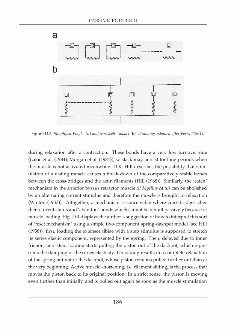
PASSIVE FORCES II

a

b

Figure D.3: Simplified Voigt - (a) and Maxwell - model (b). Drawings adapted after Ferry (1961).

during relaxation after a contraction. These bonds have a very low turnover rate(Lakie et al. (1984); Morgan et al. (1984)), so slack may persist for long periods whenthe muscle is not activated meanwhile. D.K. Hill describes the possibility that stim-ulation of a resting muscle causes a break-down of the comparatively stable bondsbetween the cross-bridges and the actin filaments (Hill (1968)). Similarly, the ‘catch´mechanism in the anterior byssus retractor muscle ofMytilus edulis can be abolishedby an alternating current stimulus and therefore the muscle is brought to relaxation(Winton (1937)). Altogether, a mechanism is conceivable where cross-bridges altertheir current status and ‘abandon´ bonds which cannot be rebuilt passively because ofmuscle loading. Fig. D.4 displays the author´s suggestion of how to interpret this sortof ‘reset mechanism´ using a simple two-component spring-dashpot model (see Hill(1938)): first, loading the extensor tibiae with a step stimulus is supposed to stretchits series elastic component, represented by the spring. Then, delayed due to innerfriction, persistent loading starts pulling the piston out of the dashpot, which repre-sents the damping of the series elasticity. Unloading results in a complete relaxationof the spring but not of the dashpot, whose piston remains pulled further out than atthe very beginning. Active muscle shortening, i.e. filament sliding, is the process thatmoves the piston back to its original position. In a strict sense, the piston is movingeven further than initially, and is pulled out again as soon as the muscle stimulation

186

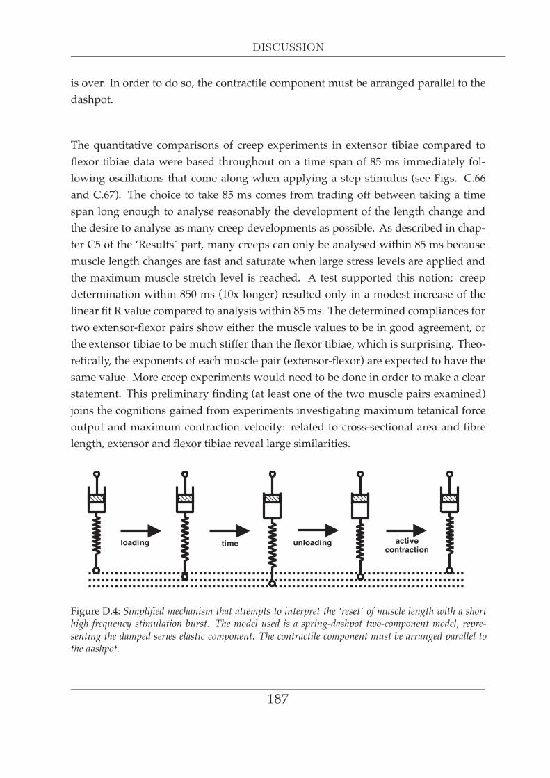
DISCUSSION

is over. In order to do so, the contractile component must be arranged parallel to thedashpot.

The quantitative comparisons of creep experiments in extensor tibiae compared toflexor tibiae data were based throughout on a time span of 85 ms immediately fol-lowing oscillations that come along when applying a step stimulus (see Figs. C.66and C.67). The choice to take 85 ms comes from trading off between taking a timespan long enough to analyse reasonably the development of the length change andthe desire to analyse as many creep developments as possible. As described in chap-ter C5 of the ‘Results´ part, many creeps can only be analysed within 85 ms becausemuscle length changes are fast and saturate when large stress levels are applied andthe maximum muscle stretch level is reached. A test supported this notion: creepdetermination within 850 ms (10x longer) resulted only in a modest increase of thelinear fit R value compared to analysis within 85 ms. The determined compliances fortwo extensor-flexor pairs show either the muscle values to be in good agreement, orthe extensor tibiae to be much stiffer than the flexor tibiae, which is surprising. Theo-retically, the exponents of each muscle pair (extensor-flexor) are expected to have thesame value. More creep experiments would need to be done in order to make a clearstatement. This preliminary finding (at least one of the two muscle pairs examined)joins the cognitions gained from experiments investigating maximum tetanical forceoutput and maximum contraction velocity: related to cross-sectional area and fibrelength, extensor and flexor tibiae reveal large similarities.

loading unloadingtime activecontraction

Figure D.4: Simplified mechanism that attempts to interpret the ‘reset´ of muscle length with a shorthigh frequency stimulation burst. The model used is a spring-dashpot two-component model, repre-senting the damped series elastic component. The contractile component must be arranged parallel tothe dashpot.

187

FORCE GENERATION UNDER NATURAL FT JOINT MOVEMENT PATTERNS

The linear theory of distributed relaxation with a power-function characteristic leadsto a common exponent k at force step application in the creep experiment (lengthL = C · tk) and for the relaxation after a length step (force P = C · t−k). k is the slopeof the linear development when applied double logarithmically. This could not beverified in the measurements shown in chapters C3 and C5. This fact may suggest theexistence of further nonlinearities in this system.

D6 Force generation under naturally occuring FTjoint movement patterns

SummaryInvestigation of extensor tibiae force increase (fitted with an exponential RC-type

growth function) and relaxation (fitted with an exponential decay function) dynamicsbefore, during and after muscle stretch and release gave several results: force increasetime constants change only little whereas relaxation time constants are much more af-fected by the muscle length changes, maximal developed force P0 confirms what onewould expect from the extensor tibiae force-length characteristic described in chapterC2. Exerted forces of actively shortened extensor tibiae muscles in response to rampsmimicking middle leg stance phase are dependent from the muscle´s activation state.From about 100 mN occuring 100 ms before the last stimulation pulse to 40 mNwhenramps start right after the last pulse to about 80 ms after the last pulse, the muscledevelops force that diminishes linearly with time after the end of stimulation. As ex-pected from Hill experiments at loads > P0, maximal developed force increases withramp velocity as it is lengthened during active contraction. Video tracking of tibialmovements in response to extensor and flexor tibiae stimulation reveals FT joint an-gular displacement to be pulse number dependent and the flexor tibiae to developlarger maximal shortening velocities than the extensor tibiae. When tibia movementwas blocked with an obstacle, extensor tibiae relaxation dynamics changed with in-creasing pulse number. The combination of history - dependent isometric extensortibiae force relaxation dynamics with passive dynamic flexor forces could reproducethe different time courses of the tibial relaxation movements observed. This calcula-

188

DISCUSSION

tion suggests the FT joint to be a mainly muscle-dominated system.

DiscussionIn integrated daily-life movement, skeletal muscle contractions are most often dy-

namic and of short duration (Ettema and Meijer (2000)). However, so-called ‘historyof contraction phenomena´ like stretch-induced force enhancement or shortening-induced force depression cannot satisfyingly be modelled with the classic Hill model.For instance, passive prestretch results in force enhancement of the extensor muscle178 in the cockroach Blaberus discoidalis (Ahn et al. (2006)). The cat soleusmuscle bearssteady-state force enhancement following active stretching, which can be abolishedinstantaneously by shortening-stretching the passive muscle by an equivalent to theactive stretch magnitude (Herzog et al. (2003)). As described in chapter D3, cross-bridges continously detach and reattach during progress of a muscle stretch. Duringsteady lengthening of single muscle fibres in Rana temporaria, the half-sarcomere stiff-ness becomes 1.25 times the isometric value (Linari et al. (2000)), similar to the resultsfound in Rana esculenta (Lombardi and Piazzesi (1990); Piazzesi et al. (1992)), and thecross-bridge number rises to 1.8 times the original isometric value. This explains whyafter-stretch potentiation shows stiffness to remain on average 12 % higher. Con-traction 2 (for the numbering, see Fig. C.68) in Fig. C.72c(ii)) demonstrates that themaximum force value arising from stretching with fast ramps (0.5 and 0.75 mms ) canbecome as high as almost 150%. The slower the stretch, the less the eccentric forceproduction (about 105% Pmax at ramp stretch of 0.1 mm

s and 135 - 150% Pmax at 0.5- 0.75 mm

s ): this is exactly what the results in chapter C4, Fig. C.52 would predictbecause of the course of the F-V curve at negative velocities. At , values of can be ex-pected (see Fig. C.52). The amount of eccentric force that a muscle or a musclegroupcan provide was already discussed in chapter D4: the kangaroo rat uses up to 175%of its maximum isometric force (Biewener et al. (1988)). In this case, the animal relieson the force enhancement that is involved with eccentric contractions, otherwise itslocomotion behaviour would have to be different. Whether the stick insect actuallytakes advantage of this force enhancement is unclear. From the cockroach, we knowthat maximum power output of cockroach extensor muscles was attained with activa-tion beginning during muscle lengthening: early activation (involving active stretch)increases muscle stiffness and facilitates storage of strain energy in tendons and cuti-cle (Full et al. (1998)). The variation of isometric force at rest (contraction 1) is within

189

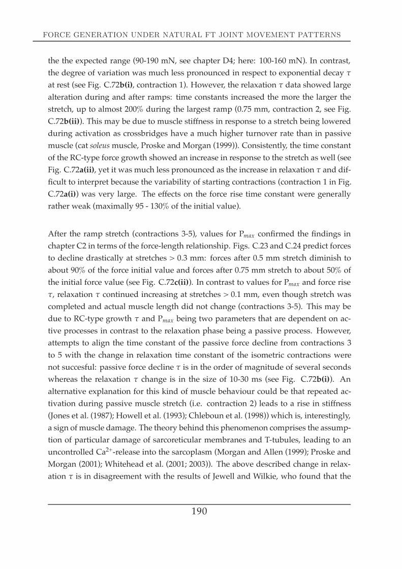
FORCE GENERATION UNDER NATURAL FT JOINT MOVEMENT PATTERNS

the the expected range (90-190 mN, see chapter D4; here: 100-160 mN). In contrast,the degree of variation was much less pronounced in respect to exponential decay τ

at rest (see Fig. C.72b(i), contraction 1). However, the relaxation τ data showed largealteration during and after ramps: time constants increased the more the larger thestretch, up to almost 200% during the largest ramp (0.75 mm, contraction 2, see Fig.C.72b(ii)). This may be due to muscle stiffness in response to a stretch being loweredduring activation as crossbridges have a much higher turnover rate than in passivemuscle (cat soleusmuscle, Proske and Morgan (1999)). Consistently, the time constantof the RC-type force growth showed an increase in response to the stretch as well (seeFig. C.72a(ii), yet it was much less pronounced as the increase in relaxation τ and dif-ficult to interpret because the variability of starting contractions (contraction 1 in Fig.C.72a(i)) was very large. The effects on the force rise time constant were generallyrather weak (maximally 95 - 130% of the initial value).

After the ramp stretch (contractions 3-5), values for Pmax confirmed the findings inchapter C2 in terms of the force-length relationship. Figs. C.23 and C.24 predict forcesto decline drastically at stretches > 0.3 mm: forces after 0.5 mm stretch diminish toabout 90% of the force initial value and forces after 0.75 mm stretch to about 50% ofthe initial force value (see Fig. C.72c(ii)). In contrast to values for Pmax and force riseτ, relaxation τ continued increasing at stretches > 0.1 mm, even though stretch wascompleted and actual muscle length did not change (contractions 3-5). This may bedue to RC-type growth τ and Pmax being two parameters that are dependent on ac-tive processes in contrast to the relaxation phase being a passive process. However,attempts to align the time constant of the passive force decline from contractions 3to 5 with the change in relaxation time constant of the isometric contractions werenot succesful: passive force decline τ is in the order of magnitude of several secondswhereas the relaxation τ change is in the size of 10-30 ms (see Fig. C.72b(i)). Analternative explanation for this kind of muscle behaviour could be that repeated ac-tivation during passive muscle stretch (i.e. contraction 2) leads to a rise in stiffness(Jones et al. (1987); Howell et al. (1993); Chleboun et al. (1998)) which is, interestingly,a sign of muscle damage. The theory behind this phenomenon comprises the assump-tion of particular damage of sarcoreticular membranes and T-tubules, leading to anuncontrolled Ca2+-release into the sarcoplasm (Morgan and Allen (1999); Proske andMorgan (2001); Whitehead et al. (2001; 2003)). The above described change in relax-ation τ is in disagreement with the results of Jewell and Wilkie, who found that the

190

DISCUSSION

decay constant was independent of the sequence of changes in length and tensionthat the muscle had undergone (sartoriusmuscle in Rana temporaria, Jewell andWilkie(1960)).

From experiments on the cat soleus muscle, it is known that full slack will developwhen the muscle is held at the longer length for several seconds before returning tostart length (Morgan et al. (1984)). Subsequent activation is lower than originally atthe same length because of both the slow rate of cross-bridge formation and the de-layed take-up time of the slack, so the muscle reveals to be more compliant (Proskeand Morgan (1999)). This might explain the ongoing alterations in τ of the exponen-tial RC-type growth and Pmax (see Fig. C.72a(i), a(ii), c(i), c(ii)) from contractions 7 to10. Relative Pmax - values at contraction 7 (right after the descending ramp moving tooriginal length) deviate from the relative initial Pmax- value at contraction 1: Pmax isclose to 100% after the slowest ramp (0.1 mms ), close to 90% at 0.25

mms , between 80 and

90% at 0.5 mms and below 80% after the fastest ramp (0.75mms ), see Fig. C.72c(ii). Thus,

the data provide evidence for the existence of a force-velocity history phenomenonthat modulates thin filament activation, which could be already demonstrated to oc-cur in frog muscle: the rate of force development after muscle fibre shortening wasfound to be increased after a slow ramp (and thus a larger isotonic force) comparedto a fast ramp involving a smaller isotonic force (tibialis anterior muscle in Rana tem-poraria, Vandenboom et al. (2002)). Relaxation τs were larger after the ramp down(contraction 6) compared to the initial value (contraction 1) and kept increasing afterthe largest ramps (red and green traces, contractions 7 to 10). According to Proskeet al. (1993), muscle slack that might occur after the relaxation ramp should be abol-ished after the first muscle stimulation, i.e. contraction 7. However, Pmax and timeconstants of both relaxation and force increase do not reach their initial values withinthe three following stimulations (contactions 8-10). This is in good agreement withdata from Ahn and colleagues, who could show that active shortening leads to forcedepression (extensor muscle 179 in Blaberus discoidalis, Ahn et al. (2006)).

In order to investigate the interaction of muscle relaxation forces and the properties ofthe Hill-hyperbola at forces > Pmax, stretch ramps were applied at different times dur-ing or briefly following stimulation of the extensor tibiae (see Figs. C.73, C.74, C.76,C.75). These ramps were supposed to mimick flexor activity during stance phase. The

191

FORCE GENERATION UNDER NATURAL FT JOINT MOVEMENT PATTERNS

transition from swing to stance features co-contraction in terms of an extensor andflexor tibiae activity overlap, which could be demonstrated to occur in the stick insectsingle leg preparation (Cuniculina impigra, Fischer et al. (2001)). Stiffness at step transi-tions is an important part of a successful control strategy used for dynamically stablethree-dimensional hopping and running robots (Raibert et al. (1984); Jindrich and Full(2002)). Antagonistic muscle co-contraction attributable to longmuscle time constantsfacilitates substantial load compensation (Zakotnik et al. (2006)), like in the stick insect(see Figs. C.16 and C.18 in chapter C2 and Hooper et al. (2007a)). Maximal extensormuscle excursions during stance can be calculated using the maximal FT-joint deflec-tion values mentioned in chapter D3 (70.8 - 90.6° (N=3, v. Uckermann and Büschges(2008)), starting at either 140° or 160° FT-joint angle, resulting in deflections of 0.27mm minimally and 0.4 mm maximally. Cycle duration in a freely moving animal is0.3 - 2 s (Bässler (1983); Fischer et al. (2001)). In both single-leg walking (Gabriel andBüschges (2007)) and intact tetrapod gait walking (Graham and Cruse (1981); Bässler(1983)), only stance phase depends on cycle period (Hooper et al. (2006)). That is,as swing phase duration is independent from walking speed (tetrapod walk of adultstick insects, Wendler (1964); Graham (1972); Bässler (1983)), stance duration can beas variable as 0.19 - 1.89 s, when calculated with a mean swing duration of 112 ms(free walking, Graham and Cruse (1981)). Thus, extensor tibiae stretching velocitiesduring stance can range from 0.14 to 2.13 mm

s in a physiological context. Hence, thestretching velocities used during or following extensor tibiae shortening of 0.33 to1.32 mm

s are close to mimick a physiological situation (see Fig. C.75a and b). Thisdetermination is the basis for the assessment of the forces and the times obtained:up to 80 ms after stimulation end, the extensor tibiae exerts force. Consistent withthe extensor tibiae Hill-curve at negative velocities (see Fig. C.52), the velocity of theramp stretch is reflected in the amount of force generated (see Fig. C.75b). In a similarexperimental arrangement, Grillner and Udo demonstrated that the stiffness of a con-tracting soleusmuscle in the cat can account for the tension increase in the steep linearpart of the stretch reflex up to maximum physiological extension (Grillner and Udo(1971)). They saw that the steep and almost linear part of the active tension increasestarts at shorter muscle lengths as the stimulus frequency is changed (Grillner (1972)).The forces measured in Fig. C.75a and b are presumably highly relevant for the stickinsect´s behaviour, as co-contraction of antagonistic muscles is known to cause sig-nificant stiffness of the limb (Schistocerca gregaria, Zakotnik et al. (2006)). From thecockroach, it is reported, that co-contraction helps adapting to different surface com-

192

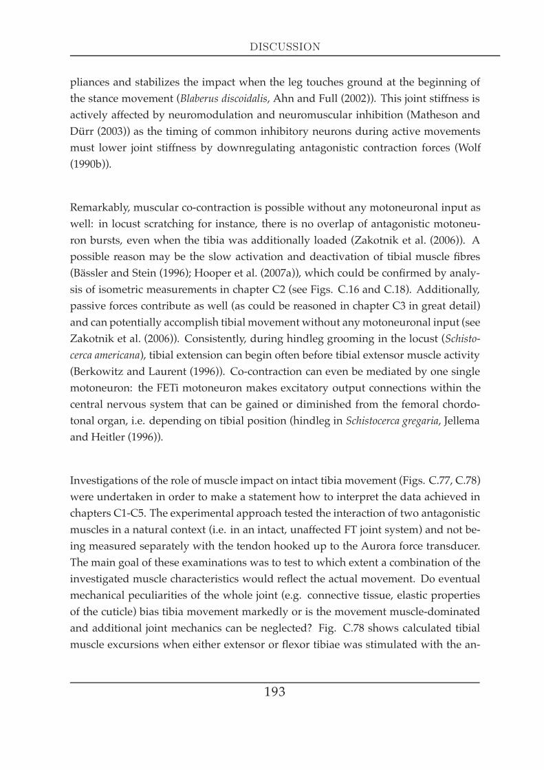
DISCUSSION

pliances and stabilizes the impact when the leg touches ground at the beginning ofthe stance movement (Blaberus discoidalis, Ahn and Full (2002)). This joint stiffness isactively affected by neuromodulation and neuromuscular inhibition (Matheson andDürr (2003)) as the timing of common inhibitory neurons during active movementsmust lower joint stiffness by downregulating antagonistic contraction forces (Wolf(1990b)).

Remarkably, muscular co-contraction is possible without any motoneuronal input aswell: in locust scratching for instance, there is no overlap of antagonistic motoneu-ron bursts, even when the tibia was additionally loaded (Zakotnik et al. (2006)). Apossible reason may be the slow activation and deactivation of tibial muscle fibres(Bässler and Stein (1996); Hooper et al. (2007a)), which could be confirmed by analy-sis of isometric measurements in chapter C2 (see Figs. C.16 and C.18). Additionally,passive forces contribute as well (as could be reasoned in chapter C3 in great detail)and can potentially accomplish tibial movement without anymotoneuronal input (seeZakotnik et al. (2006)). Consistently, during hindleg grooming in the locust (Schisto-cerca americana), tibial extension can begin often before tibial extensor muscle activity(Berkowitz and Laurent (1996)). Co-contraction can even be mediated by one singlemotoneuron: the FETi motoneuron makes excitatory output connections within thecentral nervous system that can be gained or diminished from the femoral chordo-tonal organ, i.e. depending on tibial position (hindleg in Schistocerca gregaria, Jellemaand Heitler (1996)).

Investigations of the role of muscle impact on intact tibia movement (Figs. C.77, C.78)were undertaken in order to make a statement how to interpret the data achieved inchapters C1-C5. The experimental approach tested the interaction of two antagonisticmuscles in a natural context (i.e. in an intact, unaffected FT joint system) and not be-ing measured separately with the tendon hooked up to the Aurora force transducer.The main goal of these examinations was to test to which extent a combination of theinvestigated muscle characteristics would reflect the actual movement. Do eventualmechanical peculiarities of the whole joint (e.g. connective tissue, elastic propertiesof the cuticle) bias tibia movement markedly or is the movement muscle-dominatedand additional joint mechanics can be neglected? Fig. C.78 shows calculated tibialmuscle excursions when either extensor or flexor tibiae was stimulated with the an-

193

FORCE GENERATION UNDER NATURAL FT JOINT MOVEMENT PATTERNS

tagonistical motoneurons being either crushed or cut. A maximum extensor tibiaeshortening velocity of 2.6 mms is within the range of expected velocities when the ap-plied load is 10 - 40 mN (see Fig. C.50 and Tab. C.7), which would correspond to thedynamically generated passive flexor force that would occur during tibia extension.However, maximum flexor tibiae shortening velocity is with 8.3 mms in a range of ve-locities that would be expected in a completely unloaded situation (see C.51 and Tab.C.8), where no passive extensor force would be present. This surprisingly high valueis hard to explain as the CI1- axon, that might have facilitated flexor tibiae shorteningdue to inhibition of dually and triply innervated extensor tibiae fibres (Bässler et al.(1996)), was either crushed or cut and was not stimulated extracellularly.

Aswas shown in chapter C4, average FETi spike number from 87 putative steps is 44.2± 20.0 per step-like movement (see Fig. C.41). The rather large standard deviation in-dicates that FETi motoneuronal spiking is highly variable. Steps with up to 180 spikescan occur and therefore the use of the term ‘step-like movement´ seems more appro-priate as it seems to be a fine line between walking and searching movements. ‘Activesensing´ might be an alternative way to describe this kind of behaviour (Hooper et al.(2006)), a conclusion that is consistent with the lack of clean separation between clearsteps and clear searches in Cuniculina impigra (Bässler (1993b)) and which is also con-sistent with the fact that a single artificial network is able to produce both sings andsearches (Dürr (2001)). Although most step-like movements will be carried out withless than 60 FETi motoneuron action potentials (see mean linearised extensor tibiaemucle burst in Hooper et al. (2007a)), much larger spike-numbers do occur as well(Hooper et al. (2007b)), which shows that the muscular system has to be able to dealwith the changes involved (e.g. relaxation kinetics), as described in chapter C2 andC6. Extensor tibiae bursts routinely exceed spike numbers of 40 to 60 spikes Hooperet al. (2007b)). Thus, stimulation of 20 to 140 pulses seemed to be a reasonable rangeof stimulation input to test physiological motoneuronal output on its effect in respectto post-stimulational relaxation dynamics (see Figs. C.18, C.79, C.80, C.81).

The fact that the time course of passive flexor tibiae torque subtracted from active iso-metric extensor tibiae torque can satisfyingly well reproduce videotaped intact tibiamovement in response to different extensor tibiae stimulation levels clarifies onemainissue. It points out that the above made comparison of the FT-joint with the muscle-

194

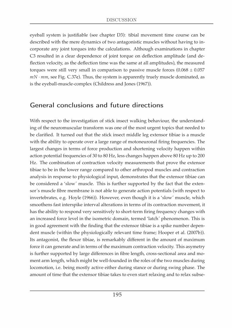
DISCUSSION

eyeball system is justifiable (see chapter D3): tibial movement time course can bedescribed with the mere dynamics of two antagonistic muscles without having to in-corporate any joint torques into the calculations. Although examinations in chapterC3 resulted in a clear dependence of joint torque on deflection amplitude (and de-flection velocity, as the deflection time was the same at all amplitudes), the measuredtorques were still very small in comparison to passive muscle forces (0.068 ± 0.057mN ·mm, see Fig. C.37c). Thus, the system is apparently truely muscle dominated, asis the eyeball-muscle-complex (Childress and Jones (1967)).

General conclusions and future directions

With respect to the investigation of stick insect walking behaviour, the understand-ing of the neuromuscular transform was one of the most urgent topics that needed tobe clarified. It turned out that the stick insect middle leg extensor tibiae is a musclewith the ability to operate over a large range of motoneuronal firing frequencies. Thelargest changes in terms of force production and shortening velocity happen withinaction potential frequencies of 30 to 80 Hz, less changes happen above 80 Hz up to 200Hz. The combination of contraction velocity measurements that prove the extensortibiae to be in the lower range compared to other arthropod muscles and contractionanalysis in response to physiological input, demonstrates that the extensor tibiae canbe considered a ‘slow´ muscle. This is further supported by the fact that the exten-sor´s muscle fibre membrane is not able to generate action potentials (with respect toinvertebrates, e.g. Hoyle (1966)). However, even though it is a ‘slow´ muscle, whichsmoothens fast interspike interval alterations in terms of its contraction movement, ithas the ability to respond very sensitively to short-term firing frequency changes withan increased force level in the isometric domain, termed ‘latch´ phenomenon. This isin good agreement with the finding that the extensor tibiae is a spike number depen-dent muscle (within the physiologically relevant time frame; Hooper et al. (2007b)).Its antagonist, the flexor tibiae, is remarkably different in the amount of maximumforce it can generate and in terms of the maximum contraction velocity. This asymetryis further supported by large differences in fibre length, cross-sectional area and mo-ment arm length, which might be well-founded in the roles of the two muscles duringlocomotion, i.e. being mostly active either during stance or during swing phase. Theamount of time that the extensor tibiae takes to even start relaxing and to relax subse-

195

quently gives evidence that theremust be a high level of stiffness at the transition fromswing to stance, as the rest of these actively generated forces need to be overcome bythe flexor tibiae. Additionally, the large dynamically generated passive muscle forcesthat occur when the antagonist shortens (either extensor or flexor tibiae), contributeas well to a large stiffness at the step transitions. In this context, the CI motoneurons(CI1 for the extensor tibiae and CI2 and CI3 for the flexor tibiae) are very likely to playa major role in facilitating antagonistic shortening. Hence, investigations combiningCI stimulation with force and length measurements are certainly a task for furtherexaminations in the future. A conceivable experimental approach could comprisenl2 or nl5 stimulation (both containing the CI1 axon) together with nl3 recording (inorder to control successful CI1 stimulation) while measuring extensor tibiae force inresponse to stretches and relaxations of different amplitude and velocity. The role ofthe CI1 neuron in force reduction of dually and triply innervated extensor tibiae fibres(see Bässler et al. (1996)) could also be an interesting future project: the CI1 neuron ismost likely responsible for the modest differences observed between full recruitmentof all three motoneurons or only partial recruitment (see ‘Materials and Methods´ sec-tion). Another urgent topic would be the examination of P0 and V0 of the musclesin other leg joints like the thorax-coxa joint (protractor and retractor coxae) and thecoxa-trochanter joint (depressor and levator trochanteris). Similar to the flexor tibiae,investigations of these muscles are limited by the existence of a large number of mo-toneurons (Goldammer et al. (2007)), which cause a problem in terms of a reasonableextracellular stimulation. In this context, measuring fibre and sarcomere lengths ofthese muscles could help comparing those muscles in terms of their maximal contrac-tion velocities V0 (see Thuma (2007)) just by comparing their structural anatomy. Thepreliminary determinations of extensor and flexor tibiae sarcomere lengths need to befinalised.

196

Appendix

197

APPENDIX

1 Spike2 scripts

The following set of scripts represents a selection of themost important scripts writtenfor either conductance of the experiments or analysis of the data presented in thisthesis. Comments (written after semicolons on the right side) and output dialogs aremostly in German.

1.1 Sequencer scripts

Script to stretch and stimulate muscle in order to obtain an active force -length curve

Letters ‘a´ to ‘e´ initiate individual subscripts to stimulate the nerve (nl3) with pulseseries of different frequency (single pulse, 30, 50, 80, 200 Hz). Letters ‘A´ to ‘C´ initiateindividual ramps to stretch the muscle starting from -0.75 mm to -0.3 mm (0 mm ∼=90° FT-angle) with 0.15 mm ramps of 1.5 s duration. Only a selection of subscripts isshown.

SET 0.050 1 0 ; Get rate & scaling OK

VAR V45,LoopC=0 ; Define variable for section loops

VAR V46,RampC=0 ; Define variable for ramp loops

VAR V47,DelayC=0 ; Define variable for delay loops

VAR V52,count=0

DAC 0,0

DAC 1,0

HALT

’a DAC 0,5; Einzelreiz

PULS1: DELAY s(0.0005)-1 ; definiert Pulsdauer (0.5ms)

DAC 0,0 ;Pulsende

HALT

198

APPENDIX

’b MOVI count,30 ; 30Hz

PULS30: DAC 0,5

DELAY s(0.0005)-1 ; definiert Pulsdauer (0.5ms)

DAC 0,0 ;Pulsende

DELAY s(0.032833)-1 ; definiert Abstand zwischen Pulsen

DBNZ count,puls30 ; loop

HALT

’c MOVI count, 50 ; 50Hz

PULS50: DAC 0,5

DELAY s(0.0005)-1 ; definiert Pulsdauer (0.5ms)

DAC 0,0 ;Pulsende

DELAY s(0.0195)-1 ; definiert Abstand zwischen Pulsen

DBNZ count,puls50 ; loop

HALT

’d MOVI count, 80 ; 80Hz

PULS80: DAC 0,5

DELAY s(0.0005)-1 ; definiert Pulsdauer (0.5ms)

DAC 0,0 ;Pulsende

DELAY s(0.012)-1 ; definiert Abstand zwischen Pulsen

DBNZ count,puls80 ; loop

HALT

’e MOVI count, 200; 200Hz

PULS200: DAC 0,5

DELAY s(0.0005)-1 ; definiert Pulsdauer (0.5ms)

DAC 0,0 ;Pulsende

DELAY s(0.0045)-1 ; definiert Abstand zwischen Pulsen

DBNZ count,puls200 ; loop

HALT

EA: ’A DIGOUT [......00] ; zu -0.6 mm

DAC 1,-1.5 ; Start point for ramp

MOVI RampC,29999 ; Loop count for ramp

RA0: ADDAC 1,1.0001e-005 ; Ramp the DAC

DBNZ RampC,RA0 ; Keep going till ramp done

199

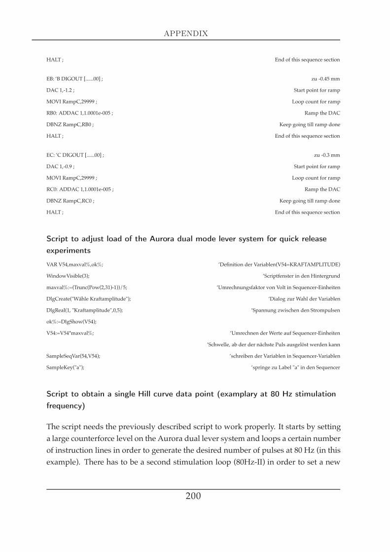
APPENDIX

HALT ; End of this sequence section

EB: ’B DIGOUT [......00] ; zu -0.45 mm

DAC 1,-1.2 ; Start point for ramp

MOVI RampC,29999 ; Loop count for ramp

RB0: ADDAC 1,1.0001e-005 ; Ramp the DAC

DBNZ RampC,RB0 ; Keep going till ramp done

HALT ; End of this sequence section

EC: ’C DIGOUT [......00] ; zu -0.3 mm

DAC 1,-0.9 ; Start point for ramp

MOVI RampC,29999 ; Loop count for ramp

RC0: ADDAC 1,1.0001e-005 ; Ramp the DAC

DBNZ RampC,RC0 ; Keep going till ramp done

HALT ; End of this sequence section

Script to adjust load of the Aurora dual mode lever system for quick releaseexperiments

VAR V54,maxval%,ok%; ’Definition der Variablen(V54=KRAFTAMPLITUDE)

WindowVisible(3); ’Scriptfenster in den Hintergrund

maxval%:=(Trunc(Pow(2,31)-1))/5; ’Umrechnungsfaktor von Volt in Sequencer-Einheiten

DlgCreate("Wähle Kraftamplitude"); ’Dialog zur Wahl der Variablen

DlgReal(1, "Kraftamplitude",0,5); ’Spannung zwischen den Strompulsen

ok%:=DlgShow(V54);

V54:=V54*maxval%; ’Umrechnen der Werte auf Sequencer-Einheiten

’Schwelle, ab der der nächste Puls ausgelöst werden kann

SampleSeqVar(54,V54); ’schreiben der Variablen in Sequencer-Variablen

SampleKey("a"); ’springe zu Label "a" in den Sequencer

Script to obtain a single Hill curve data point (examplary at 80 Hz stimulationfrequency)

The script needs the previously described script to work properly. It starts by settinga large counterforce level on the Aurora dual lever system and loops a certain numberof instruction lines in order to generate the desired number of pulses at 80 Hz (in thisexample). There has to be a second stimulation loop (80Hz-II) in order to set a new

200

APPENDIX

counterforce level (V54) between the two loops.

’a DIGOUT [......00] ; Hill-80Hz

DAC 1,5

MOVI count,79 ; 80Hz-I

PULS15: DAC 0,5

DELAY ms(0.5)

DAC 0,0

DELAY s(0.0115)

DBNZ count,puls15

DAC 0,5

DELAY ms(0.5)

DAC 0,0

DELAY s(0.0054)

DAC 1,V54 ; Kraftamplitude

DELAY s(0.006)

MOVI count,40 ; 80Hz-II

PULS16: DAC 0,5

DELAY ms(0.5)

DAC 0,0

DELAY s(0.0115)

DBNZ count,puls16

DELAY s(1.5)

DAC 1,5

HALT

Script to stretch muscle at particular times before or after the end ofstimulation

The essential feature of this sequencer script is the output instruction ‘Call´, whichsaves the next step number to a return stack and jumps to the labelled instruction.That is, the script provides the oppurtunity to memorise a value that can be used toinitiate a chain of instructions starting from this value.

201

APPENDIX

SET 0.100 1 0 ; Get rate & scaling OK

VAR V1,poBase ; Position OUT start level

VAR V2,piBase ; Position IN start level

VAR V3,piCurr ; Current IN position

VAR V58,poCurr ; Current OUT position

VAR V5,deltaPi ; IN Differenz (piBase-piCurr)

VAR V6,tmp

VAR V7,rSlopeA=VDAC32(0.0042)

VAR V8,rISlopeA=VDAC32(2)

VAR V9,loopCnt

VAR V11,delayRes=0

VAR V12,delayStd=2000 ; time after stimulation start

VAR V13,delaySub=0 ; subtracted time from V12: controls the time of the ramp start

VAR V14,rampc=0

VAR V15,Stufe ; this value determines the ramp speed of the muscle stretch

VAR V16,tem

VAR V17,delayS2=0

VAR V50,force2=2

VAR V33,piConAmp=0

DAC 0,0.24

DAC 1,0

HALT ;

’X CALL READPI ; gereizt

MOV piBase,piCurr

DIGOUT [......01]

DIGOUT [......00]

DELAY delayStd

DELAY delaySub ; 0-x ms

CALL READPI

MOV piConAmp,piCurr

MOV deltaPi,piBase

SUB deltaPi,piCurr

NEG deltaPi,deltaPi

DAC 1,deltaPi

DAC 0,0.3

202

APPENDIX

ADDAC 1,Stufe ; VAR15: 0.00045 - 0.0018

DAC 0,0.5

ADDAC 1,Stufe

DAC 0,0.7

ADDAC 1,Stufe

DAC 0,0.9

ADDAC 1,Stufe

DAC 0,1.2

ADDAC 1,Stufe

DAC 0,1.5

ADDAC 1,Stufe

DAC 0,2

DELAY delayS2 ; x+y ms

RAMPX: ADDAC 1,Stufe ; VAR15: 0.00045 - 0.0018

CALL READPI

BLT piCurr,piBase,rampx

DAC 1,0

DELAY s(2)

DAC 0,0.24

HALT

READPI: CHAN tmp,3 ; ; reads the value of channel 3 (16 bit) into the piCurr variable, additionally

MULI tmp,65536 ; ; scales the input to into the DAC value range (32 bit)

MOV piCurr,tmp

RETURN

Script to stimulate the nerve with a physiological pattern

The following lines combine two different scripts: ‘PlayWaveAdd´ accomplishes ac-cess to an already existing waveform file (in this example: from 0s to 165s of therecording termed ‘PhysCo´) and calls this sequence ‘A´. The output of this sequence(‘A´) can be initiated subsequently by ‘WAVEGO´.

PlayWaveAdd ("A","PhysCo",0,0,165,3);

’P DIGOUT [......00] ; physiologische Stim. ISOTONISCH

DAC 1,0.8 ; 40 mN counterforce

203

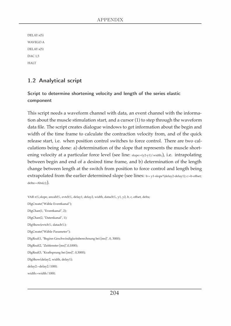
APPENDIX

DELAY s(5)

WAVEGOA

DELAY s(5)

DAC 1,5

HALT

1.2 Analytical script

Script to determine shortening velocity and length of the series elasticcomponent

This script needs a waveform channel with data, an event channel with the informa-tion about the muscle stimulation start, and a cursor (1) to step through the waveformdata file. The script creates dialogue windows to get information about the begin andwidth of the time frame to calculate the contraction velocity from, and of the quickrelease start, i.e. when position control switches to force control. There are two cal-culations being done: a) determination of the slope that represents the muscle short-ening velocity at a particular force level (see line: slope:=(y2-y1)/width;), i.e. intrapolatingbetween begin and end of a desired time frame, and b) determination of the lengthchange between length at the switch from position to force control and length beingextrapolated from the earlier determined slope (see lines: b:= y1-slope*(delay2-delay1); c:=b-offset;delta:=Abs(c);).

VAR n%,slope, anzahl%, evtch%, delay1, delay2, width, datach%, y1, y2, b, c, offset, delta;

DlgCreate("Wähle Eventkanal");

DlgChan(1, "Eventkanal", 2);

DlgChan(2, "Datenkanal", 1);

DlgShow(evtch%, datach%);

DlgCreate("Wähle Parameter");

DlgReal(1, "Beginn Geschwindigkeitsberechnung bei [ms]", 0, 3000);

DlgReal(2, "Zeitfenster [ms]",0,1000);

DlgReal(3, "Kraftsprung bei [ms]", 0,3000);

DlgShow(delay2, width, delay1);

delay2:=delay2/1000;

width:=width/1000;

204

REFERENCES

delay1:=delay1/1000;

Cursor(1, 0);

anzahl%:=count(evtch%, 0, MaxTime());

printlog("Zeit",chr$(9), "Steigung", "erster Positionssprung");

for n%:=1 to anzahl% do

Cursor(1, Nexttime(evtch%, cursor(1)));

y1:=Chanvalue(datach%, cursor(1)+delay2);

y2:=Chanvalue(datach%, cursor(1)+delay2+width);

offset:=Chanvalue(datach%, cursor(1)+3);

slope:=(y2-y1)/width;

b:= y1-slope*(delay2-delay1);

c:=b-offset;

delta:=Abs(c);

printlog(cursor(1), slope,chr$(9), delta);

next

205

REFERENCES

ReferencesAbbot, B. and Aubert, X. (1952). The force exerted by active striated muscle during and after change oflength. J Physiol, 117(1):77–86.

Abbot, B. and Wilkie, D. (1953). The relation between velocity of shortening and the tension-lengthcurve of skeletal muscle. J Physiol, 120:214–223.

Abbot, R. (1973). Does calcium affect the rate constants ofmuscle? In 37thCold Spring Harbor Symposiumof Quantitative Biology.

Ahn, A. and Full, R. (2002). A motor and a brake: two leg extensor muscles acting at the same jointmanage energy differently in a running insect. J Exp Biol, 205:379–389.

Ahn, A., Meijer, K., and Full, R. (2006). In situ muscle power differs without varying in vitro mechan-ical properties in two insect leg muscles innervated by the same motor neuron. J Exp Biol, 209(Pt17):3370–3382.

Akay, T., Bässler, U., Gerharz, P., and Büschges, A. (2001). The role of sensory signals from the insectcoxa-trochanteral joint in controlling motor activity of the femur-tibia joint. J Neurophysiol, 85(2):594–604.

Akay, T. and Büschges, A. (2006). Load signals assist the generation of movement-dependent reflexreversal in the femur-tibia joint of stick insects. J Neurophysiol, 96(6):3532–3537.

Akay, T., Haehn, S., Schmitz, J., and Büschges, A. (2004). Signals from load sensors underlie interjointcoordination during stepping movements of the stick insect leg. J Neurophysiol, 92(1):42–51.

Alexander, R. M. (1985). The maximum forces exerted by animals. J Exp Biol, 115:231–238.Anderson, F. and Pandy, M. (1999). A dynamic optimization solution for vertical jumping in threedimensions. Comput Methods Biomech Biomed Engin, 2(3):201–231.

Armstrong, C., Huxley, A., and Julian, F. (1966). Oscillatory responses in frog skeletal muscle fibres. JPhysiol, 186:26–27.

Atwood, H. L. (1965). Excitation and inhibition in crab muscle fibres. Comp Biochem Physiol, 16(4):409–426.

Balnave, C. D. and Allen, D. G. (1996). The effect of muscle length on intracellular calcium and force insingle fibres from mouse skeletal muscle. J Physiol, 492 ( Pt 3):705–713.

Bartling, C. and Schmitz, J. (2000). Reaction to disturbances of a walking leg during stance. J Exp Biol,203:1–13.

Bässler, D., Büschges, A., Meditz, S., and Bässler, U. (1996). Correlation between muscle structureand filter characteristics of the muscle-joint system in three orthopteran insect species. J Exp Biol,199:2169–2183.

Bässler, U. (1965). Propriorezeptoren am Subcoxal- und Femur-Tibia-Gelenk der Stabheuschrecke Ca-rausius morosus und ihre Rolle bei der Wahrnehmung der Schwerkraftrichtung. Kybernetik, 2(4):168–193.

Bässler, U. (1967). Zur Regelung der Stellung des Femur-Tibia-Gelenkes bei der Stabheuschrecke Ca-rausius morosus in der Ruhe und im Lauf. Kybernetik, 4:18–26.

Bässler, U. (1972). Der Regelkreis des Kniesehnenreflexes bei der Stabheuschrecke Carausius morosus:Reaktionen auf passive Bewegungen der Tibia. Kybernetik, 12:8–20.

Bässler, U. (1974). Vom femoralen Chordotonalorgan gesteuerte Reaktionen bei der StabheuschreckeCarausius morosus: Messung der von der Tibia erzeugten Kraft im aktiven und inaktiven Tier. Ky-bernetik, 16:213–226.

206

REFERENCES

Bässler, U. (1977). Sense organs in the femur of the stick insect and their relevance to the control ofposition of the femur-tibia-joint. J Comp Physiol A, 121:99–113.

Bässler, U. (1983). Stick Insect News. Annual Supplement to Neural Basis of elementary behavior in stickinsects. No. 1-8. Springer Verl.

Bässler, U. (1993a). The femur-tibia control system of stick insects - a model system for the study of theneural basis of joint control. Brain Research Reviews, 18:207–226.

Bässler, U. (1993b). The walking- (and searching-) pattern generator of stick insects, a modular systemcomposed of reflex chains and endogenous oscillators. Biol Cybern, 69:305–317.

Bässler, U. and Büschges, A. (1998). Pattern generation for stick insect walking movements - multisen-sory control of a locomotor program. Brain Research, 27:65–88.

Bässler, U. and Stein, W. (1996). Contributions of structure and innervation pattern of the stick insectextensor tibiae muscle to the filter characteristics of the muscle-joint system. J Exp Biol, 199:2185–2198.

Bässler, U. and Storrer, J. (1980). The neural basis of the femur-tibia-control-system in the stick insectCarausius morosus. I. motoneurons of the extensor tibiae muscle. Biol Cybern, 38:107–114.

Bässler, U. and Wegner, U. (1983). Motor output of the denervated thoracic ventral nerve cord in thestick insect Carausius morosus. J. exp. Biol., 105:127–145.

Bässler, U., Wolf, H., and Stein, W. (2007). Functional recovery following manipulation of musclesand sense organs in the stick insect leg. J Comp Physiol A Neuroethol Sens Neural Behav Physiol,193(11):1151–1168.

Becht, G. and Dresden, D. (1956). Physiology of the locomotory muscles in the cockroach. Nature,17:836–837.

Becht, G., Hoyle, G., and Usherwood, P. (1960). Neuromuscular transmission in the coxal muscles ofthe cockroach. J Insect Physiol, 4:191–201.

Bennet-Clark, H. C. (1975). The energetics of the jump of the locust Schistocerca gregaria. J Exp Biol,63(1):53–83.

Bennett, M. B. and Taylor, G. C. (1995). Scaling of elastic strain energy in kangaroos and the benefits ofbeing big. Nature, 378(6552):56–59.

Berkowitz, A. and Laurent, G. (1996). Local control of leg movements and motor patterns duringgrooming in locusts. J Neurosc., 16(24):8067–8078.

Biewener, A. A., Blickhan, R., Perry, A. K., Heglund, N. C., and Taylor, C. R. (1988). Muscle forcesduring locomotion in kangaroo rats: force platform and tendon buckle measurements compared. JExp Biol, 137:191–205.

Blaschko, H., Cattell, M., and Kahn, J. (1931). On the nature of the two types of response in the neuro-muscular system of the crustacean claw. J Physiol, 73:25–35.

Blickhan, R. (1986). Stiffness of an arthropod leg joint. J Biomech, 19(5):375–384.Blickhan, R., Wagner, H., and Seyfarth, A. (2003). Recent research developments in Biomechanics. Vol. 1,chapter Brain or muscles., pages 215–245. India. Transworld Research Network, Thiru-anantha-puram (Trivandrum).

Blümel, M., Guschlbauer, C., and Büschges, A. (2008a). Muscle and joint simulation. In DFG meetingCologne: Load and force control in walking pattern generation of animals and robots: From sensors to localand global control function.

Blümel, M., Guschlbauer, C., and Büschges, A. (2008b). Muscle properties in leg step control. InMBIworkshop 4/2008: Neuromechanics of locomotion.

Blümel, M., Guschlbauer, C., Gruhn, M., Scharstein, H., and A., B. (2007a). Predicting swing phasemovements of the stick insect FT joint. In 100th annual meeting of the Deutsche Zoologische Gesellschaft(Köln).

207

REFERENCES

Blümel, M., Guschlbauer, C., Zehl, L., Hooper, S., and A., B. (2007b). Investigating stick insect extensormuscle properties: an experimentally based muscle simulation. In Proceedings of the 31st GöttingenNeurobiology conference and the 7th meeting of the German Neuroscience society.

Bodine, S. C., Roy, R. R., Eldred, E., and Edgerton, V. R. (1987). Maximal force as a function of anatom-ical features of motor units in the cat tibialis anterior. J Neurophysiol, 57(6):1730–1745.

Borgmann, A., Scharstein, H., and Buschges, A. (2007). Intersegmental coordination: the influence ofa single walking leg on the neighboring segments in the stick insect walking system. J Neurophysiol,98:1685–1696.

Boyd, I. and Davey, M. (1968). Composition of peripheral nerves. London.Brown, I. E., Cheng, E. J., and Loeb, G. E. (1999). Measured and modeled properties of mammalianskeletal muscle. II. the effects of stimulus frequency on force-length and force-velocity relationships.J Muscle Res Cell Motil, 20(7):627–643.

Brown, I. E., Kim, D. H., and Loeb, G. E. (1998). The effect of sarcomere length on triad location inintact feline caudofeomoralis muscle fibres. J Muscle Res Cell Motil, 19(5):473–477.

Brown, I. E. and Loeb, G. E. (1999). Measured and modeled properties of mammalian skeletal muscle.I. the effects of post-activation potentiation on the time course and velocity dependencies of forceproduction. J Muscle Res Cell Motil, 20(5-6):443–456.

Brown, I. E. and Loeb, G. E. (2000a). Biomechanics and neural control of movement., chapter A reductionistapproach to creating and using neuromusculoskeletal models., pages 148–163. Springer Verlag, NewYork.

Brown, I. E. and Loeb, G. E. (2000b). Measured andmodeled properties of mammalian skeletal muscle:III. the effects of stimulus frequency on stretch-induced force enhancement and shortening-inducedforce depression. J Muscle Res Cell Motil, 21(1):21–31.

Brown, I. E. and Loeb, G. E. (2000c). Measured and modeled properties of mammalian skeletal muscle:IV. dynamics of activation and deactivation. J Muscle Res Cell Motil, 21(1):33–47.

Brown, T. I., Rack, P. M., and Ross, H. F. (1982). Electromyographic responses to imposed sinusoidalmovement of the human thumb. J Physiol, 332:87–99.

Burck, H. (1988). Histologische Technik. pp. 123-124. Stuttgart, New York: Thieme Verlag.Burns, M. and Usherwood, P. (1978). Mechanical properties of locust extensor tibiae muscles. CompBiochem Physiol, 61A:85–95.

Burns, M. and Usherwood, P. (1979). The control of walking in orthoptera. II. motor neurone activityin normal free-walking animals. J Exp Biol, 79:69–98.

Burrows, M. and Wolf, H. (2002). Jumping and kicking in the false stick insect Prosarthria teretrirostris:kinematics and motor control. J Exp Biol, 205(Pt 11):1519–1530.

Büschges, A. (1995a). Plasticity of neuronal networks that control posture and movement of leg jointin insects. Verh Dtsch Zool Ges, 88:139–151.

Büschges, A. (1995b). Role of local nonspiking interneurons in the generation of rhythmic motor activ-ity in the stick insect. J Neurobiol, 27(4):488–512.

Büschges, A. (2005). Sensory control and organization of neural networks mediating coordination ofmultisegmental organs for locomotion. J Neurophysiol, 93(3):1127–1135.

Büschges, A., Kittmann, R., and Schmitz, J. (1994). Identified nonspiking interneurons in leg reflexesand during walking in the stick insect. J Comp Physiol [A], 174:685–700.

Büschges, A., Ludwar, B. C., Bucher, D., Schmidt, J., and DiCaprio, R. A. (2004). Synaptic drive con-tributing to rhythmic activation of motoneurons in the deafferented stick insect walking system. EurJ Neurosci, 19(7):1856–1862.

Büschges, A. and Schmitz, J. (1991). Nonspiking pathways antagonize the resistance reflex in thethoraco-coxal joint of stick insects. J Neurobiol, 22(3):224–237.

Cavagna, G. A. and Citterio, G. (1974). Effect of stretching on the elastic characteristics and the con-tractile component of frog striated muscle. J Physiol, 239(1):1–14.

208

REFERENCES

Childress, D. S. and Jones, R. W. (1967). Mechanics of horizontal movement of the human eye. J Physiol,188(2):273–284.

Chleboun, G. S., Howell, J. N., Conatser, R. R., and Giesey, J. J. (1998). Relationship between muscleswelling and stiffness after eccentric exercise. Med Sci Sports Exerc, 30(4):529–535.

Chow, J. W. and Darling, W. G. (1999). The maximum shortening velocity of muscle should be scaledwith activation. J Appl Physiol, 86(3):1025–1031.

Civan, M. M. and Podolsky, R. J. (1966). Contraction kinetics of striated muscle fibres following quickchanges in load. J Physiol, 184(3):511–534.

Close, R. I. (1972). Dynamic properties of mammalian skeletal muscles. Physiol Rev, 52(1):129–197.Coveney, V. A., Hunter, G. D., and Spriggs, J. (2001). Is the behaviour of the leg during oscillationlinear? J Biomech, 34(6):827–830.

Cruse, H. (1976). The function of the legs in the free walking stick insect, Carausius morosus. J CompPhysiol A, 112:235–262.

Cruse, H. (1985a). Which parameters control the leg movement of a walking insect? I. Velocity controlduring the stance phase. J Exp Biol, 116:343–355.

Cruse, H. (1985b). Which parameters control the leg movement of a walking insect? II. the start of theswing phase. J.exp.Biol., 116:357–362.

Cruse, H. and Bartling, C. (1995). Movement of joint angles in the legs of a walking insect. Carausiusmorosus. J Insect Physiol, 41:761–771.

Cruse, H. and Storrer, J. (1977). Open loop analysis of a feedback mechanism controlling the legposition in the stick insect carausius morosus: comparison between experiment and simulation.Biol.Cybern., 25:143–153.

De Haan, A. (1998). The influence of stimulation frequency on force-velocity characteristics of in siturat gastrocnemiusmuscle. J Exp Physiol, 83:77–84.

Dean, J. (1984). Control of leg protraction in the stick insect: a targeted movement showing compensa-tion for externally applied forces. J. Comp Physiol A, 155:771–781.

Debrodt, B. and Bässler, U. (1989). Motor neurones of the flexor tibiae muscle in phasmids. Zool JbPhysiol, 93:481–494.

Debrodt, B. and Bässler, U. (1990). Responses of flexor motor neurons to stimulation of the femoralchordotonal organ of the phasmid Extratosoma tiaratum. Zool. Jb. Physiol., 94:101–119.

Delcomyn, F. (1971). Computer aided analysis of a locomotor leg reflex in the cockroach Periplanetaamericana. Z vergl Physiologie, 74:427–445.

Denny-Brown, D. (1929). On the nature of postural reflexes. Proc R Soc Lond Ser B, 104:252–301.Driesang, R. and Büschges, A. (1993). The neural basis of catalepsy in the stick insect. IV. properties ofnonspiking interneurons. J.Comp.Physiol.A, 173:445–454.

Dudek, D. M. and Full, R. J. (2006). Passive mechanical properties of legs from running insects. J ExpBiol, 209(Pt 8):1502–1515.

Dürr, V. (2001). Stereotypic leg searching movements in the stick insect: kinematic analysis, behavioralcontext and simulation. J Exp Biol, 204:1589–1604.

Dürr, V., Schmitz, J., and Cruse, H. (2004). Behavior-based modelling of hexapod locomotion: linkingbiology and technical application. Arthropod Structure & Development, 33:237–250.

Edman, K. A. (1966). The relation between sarcomere length and active tension in isolated semitendi-nosus fibres of the frog. J Physiol, 183(2):407–417.

Edman, K. A. (1970). The rising phase of the active state in single skeletal muscle fibres of the frog.Acta Physiol Scand, 79(2):167–173.

Edman, K. A. (1979). The velocity of unloaded shortening and its relation to sarcomere length andisometric force in vertebrate muscle fibres. J Physiol, 291:143–159.

209

REFERENCES

Edman, K. A. (1988). Double-hyperbolic force-velocity relation in frog muscle fibres. J Physiol, 404:301–321.

Edman, K. A. and Curtin, N. A. (2001). Synchronous oscillations of length and stiffness during loadedshortening of frog muscle fibres. J Physiol, 534(Pt. 2):553–563.

Edman, K. A., Elzinga, G., and Noble, M. I. (1978). Enhancement of mechanical performance by stretchduring tetanic contractions of vertebrate skeletal muscle fibres. J Physiol, 281:139–155.

Edman, K. A. andKiessling, A. (1971). The time course of the active state in relation to sarcomere lengthand movement studied in single skeletal muscle fibres of the frog. Acta Physiol Scand, 81(2):182–196.

Edman, K. A., Mulieri, L. A., and Scubon-Mulieri, B. (1976). Non-hyperbolic force-velocity relationshipin single muscle fibres. Acta Physiol Scand, 98(2):143–156.

Edman, K. A., Månsson, A., and Caputo, C. (1997). The biphasic force-velocity relationship in frogmuscle fibres and its evaluation in terms of cross-bridge function. J Physiol, 503 ( Pt 1):141–156.

Edman, K. A. P. (2005). Contractile properties of mouse single muscle fibers, a comparison with am-phibian muscle fibers. J Exp Biol, 208(Pt 10):1905–1913.

Edman, K. A. P. and Josephson, R. K. (2007). Determinants of force rise time during isometric contrac-tion of frog muscle fibres. J Physiol, 580(Pt.3):1007–1019.

Eisenberg, E., Hill, T. L., and Chen, Y. (1980). Cross-bridge model of muscle contraction. Quantitativeanalysis. Biophys J, 29(2):195–227.

Ekeberg, Ö., Blümel, M., and Büschges, A. (2004). Dynamic simulation of insect walking. AthropodStructure and Development, 33:287–300.

Ekeberg, Ö. (2002). Modeling of interactions between neural networks and musculoskeletal system.Computional Neuroscience - Realistic modeling for Experimentalists, pages 317–335.

Endo, M. (1973). Length dependence of activation of skin muscle fibres by calcium. Cold Spring HarborSymposia on Quantitative Biology, 37:505–510.

Esteki, A. and Mansour, J. M. (1996). An experimentally based nonlinear viscoelastic model of jointpassive moment. J Biomech, 29(4):443–450.

Ettema, G. andMeijer, K. (2000). Muscle contraction history: modified hill versus an exponential decaymodel. Biol Cybern, 83:491–500.

Evans, P. and O’Shea, M. (1978). The identification of an octopaminergic neurone and the modulationof a myogenic rhythm in the locust. J Exp Biol, 73:235–260.

Evans, P. D. and O’Shea, M. (1977). An octopaminergic neurone modulates neuromuscular transmis-sion in the locust. Nature, 270(5634):257–259.

Evans, P. D. and Siegler, M. V. (1982). Octopamine mediated relaxation of maintained and catch tensionin locust skeletal muscle. J Physiol, 324:93–112.

Fenn, W. O. and Marsh, B. S. (1935). Muscular force at different speeds of shortening. J Physiol,85(3):277–297.

Ferry, J. D. (1961). Viscoelastic properties of polymers. New York, London; John Wiley & Sons, Inc.Field, L. and Pflüger, H. (1989). The femoral chordotonal organ: a bifunctional orthopteran (Locustamigratoria) sense organ? Comp. Biochem. Physiol., 93A:729–743.

Fischer, H., Schmidt, J., Haas, R., and Büschges, A. (2001). Pattern generation for walking and searchingmovements of a stick insect leg. I. Coordination of motor activity. J Neurophysiol, 85(1):341–353.

Friedrich, H. (1932). Nervenphysiologische Studien an Insekten I. Untersuchungen über das reizphys-iologische Verhalten der Extremitäten von Dixippus morosus. Z vergl Physiol, 18:536–561.

Full and Ahn (1995). Static forces and moments generated in the insect leg: comparison of a three-dimensional musculo-skeletal computer model with experimental measurements. J Exp Biol, 198(Pt6):1285–1298.

210

REFERENCES

Full, Yamauchi, and Jindrich (1995). Maximum single leg force production: cockroaches righting onphotoelastic gelatin. J Exp Biol, 198(Pt 12):2441–2452.

Full, R. (1997). Invertebrate locomotor systems. In Dantzler, W., editor, The Handbook of ComparativePhysiology, number 12, pages 853–930. Oxford University Press, Oxford.

Full, R. and Koditschek, D. (1999). Templates and anchors: neuromechanical hypotheses of leggedlocomotion on hand. J Exp Biol, 202:3325–3332.

Full, R. and Meijer, K. (1997). Metrics of natural muscle function. In Electroactive polymer actuators asartificial muscles, number 3, pages 67–83.

Full, R., Stokes, D., Ahn, A., and Josephson, R. (1998). Energy absorption during running by legmuscles in a cockroach. J Exp Biol, 201:997–1012.

Full, R. and Tu, M. (1991). Mechanics of a rapid running insect: two-, four- and six-legged locomotion.J Exp Biol, 156:215–231.

Full, R. J. and Farley, C. T. (2000). Biomechanics & neural control of posture & movement., chapter Mus-culoskeletal Dynamics in Rhythmic Systems: a comparative approach to legged locomotion., pages192–203. Springer Verlag-New York, Inc.

Funabara, D., Kanoh, S., Siegman, M. J., Butler, T. M., Hartshorne, D. J., andWatabe, S. (2005). Twitchinas a regulator of catch contraction in molluscan smooth muscle. J Muscle Res Cell Motil, 26(6-8):455–460.

Fung, Y. C. (2004). Biomechanics: mechanical properties of living tissues, chapterQuasi-linear viscoelasticityof soft tissues. Springer Science + Business Media.

Gabriel, J. (2005). Activity of leg motoneurons during single leg walking of the stick insect: From synapticinputs to motor performance. PhD thesis, University of Cologne.

Gabriel, J. and Büschges, A. (2007). Control of stepping velocity in a single insect leg during walking.Philos Transact A Math Phys Eng Sci, 365(1850):251–271.

Gabriel, J., Scharstein, H., Schmidt, J., and Büschges, A. (2003). Control of flexor motoneuron activityduring single leg walking of the stick insect on an electronically controlled treadwheel. J Neurobiol,56(3):237–251.

Godden, D. (1974). The physiological mechanism of catalepsy in the stick insect Carausius morosus Br.J Comp Physiol, 89:251–274.

Goldammer, J., Mentel, T., and Büschges, A. (2007). A tracing study of leg motoneurons in Carausiusmorosus. In 100th Annual meeting of the Deutsche Zoologische Gesellschaft (Köln) 2007.

Gordon, A. M., Huxley, A. F., and Julian, F. J. (1966a). Tension development in highly stretched verte-brate muscle fibres. J Physiol, 184(1):143–169.

Gordon, A.M., Huxley, A. F., and Julian, F. J. (1966b). The variation in isometric tension with sarcomerelength in vertebrate muscle fibres. J Physiol, 184(1):170–192.

Graham, D. (1972). A behavioural analysis of the temporal organisation of walking movements in the1st instar and adult stick insect (Carausius morosus). J Comp Physiol, 81:23–52.

Graham, D. (1983). Insects are both impeded and propelled by their legs during walking. J Exp Biol,104:129–137.

Graham, D. (1985). Pattern and control of walking in insects. InAdvances in Insect Physiology, volume 18,pages 31–140. Academic Press Inc., London.

Graham, D. and Cruse, H. (1981). Coordinated walking of stick insects on a mercury surface. J ExpBiol, 92:229–241.

Grillner, S. (1972). The role of muscle stiffness in meeting the changing postural and locomotor require-ments for force development by the ankle extensors. Acta Physiol Scand, 86(1):92–108.

Grillner, S., Parker, D., and Manira, A. E. (1998). Vertebrate locomotion–a lamprey perspective. Ann NY Acad Sci, 860:1–18.

211

REFERENCES

Grillner, S. and Udo, M. (1971). Motor unit activity and stiffness of the contracting muscle fibres in thetonic stretch reflex. Acta Physiol Scand, 81(3):422–424.

Gruhn, M., Hoffmann, O., Dübbert, M., Scharstein, H., and Büschges, A. (2006). Tethered stick insectwalking: a modified slippery surface setup with optomotor stimulation and electrical monitoring oftarsal contact. J Neurosci Methods, 158(2):195–206.

Guschlbauer, C., Scharstein, H., and Büschges, A. (2007). The extensor tibiae muscle of the stick insect:biomechanical properties of an insect walking leg muscle. J Exp Biol, 210(Pt 6):1092–1108.

Günzel, D. and Rathmayer, W. (1994). Non-uniformity of sarcomere lengths can explain the ’catch-like’effect of arthropod muscle. J Muscle Res Cell Motil, 15(5):535–546.

Haas, F., Gorb, S., and Blickhan, R. (2000). The function of resilin in beetle wings. Proc Biol Sci,267(1451):1375–1381.

Hajian, A. Z. and Howe, R. D. (1997). Identification of the mechanical impedance at the human fingertip. J Biomech Eng, 119(1):109–114.

Heide, G. and Götz, K. G. (1996). Optomotor control of course and altitude in Drosophila melanogasteris correlated with distinct activities of at least three pairs of flight steering muscles. J Exp Biol, 199(Pt8):1711–1726.

Herrel, A., Meyers, J. J., Aerts, P., and Nishikawa, K. C. (2001). Functional implications of supercon-tracting muscle in the chameleon tongue retractors. J Exp Biol, 204(Pt 21):3621–3627.

Herrel, A., Meyers, J. J., Timmermans, J.-P., and Nishikawa, K. C. (2002). Supercontracting muscle:producing tension over extreme muscle lengths. J Exp Biol, 205(Pt 15):2167–2173.

Herzog, W., Schachar, R., and Leonard, T. R. (2003). Characterization of the passive component of forceenhancement following active stretching of skeletal muscle. J Exp Biol, 206(Pt 20):3635–3643.

Hildebrand, M. (1988). Analysis of vertebrate structure. New York, Toonto: John Wiley & Sons.Hill, A. V. (1938). The heat of shortening and the dynamic constants of muscle. Proc. R. Soc. Lond. B Bio.Sci., 126:136–195.

Hill, A. V. (1949). The energetics of relaxation in a muscle twitch. Proc R Soc Lond B Biol Sci,136(883):211–219.

Hill, A. V. (1950). The dimensions of animals and their muscular dynamics. Sci. Progr., 38:209–230.Hill, D. K. (1968). Tension due to interaction between the sliding filaments in resting striated muscle.the effect of stimulation. J Physiol, 199(3):637–684.

Hodgkin, A. and Huxley, A. (1952). Currents carried by sodium and potassium ions through themembrane of the giant axon of Loligo. J Physiol, 116:449–472.

Hogan, N. (1982). Robot motion, Vol. 5, chapter Mechanical impedance control in assistive devices andmanipulators. Cambridge, MA: MIT Press.

Hooper, S., Guschlbauer, C., Blümel, M., Rosenbaum, P., Gruhn, M., Akay, T., and Büschges, A. (2009).Neural control of unloaded leg posture and of leg swing in stick insect, cockroach, andmouse differsfrom that in larger animals. submitted.

Hooper, S., Guschlbauer, C., von Uckermann, G., and Büschges, A. (2006). Natural neural output thatproduces highly variable locomotory movements. J Neurophysiol, 96(4):2072–2088.

Hooper, S. L., Guschlbauer, C., von Uckermann, G., and Buschges, A. (2007a). Slow temporal filteringmay largely explain the transformation of stick insect (carausius morosus) extensor motor neuronactivity into muscle movement. J Neurophysiol.

Hooper, S. L., Guschlbauer, C., von Uckermann, G., and Büschges, A. (2007b). Different motor neuronspike patterns produce contractions with very similar rises in graded slow muscles. J Neurophysiol,97(2):1428–1444.

Hooper, S. L., Hobbs, K. H., and Thuma, J. B. (2008). Invertebrate muscles: thin and thick filamentstructure; molecular basis of contraction and its regulation, catch and asynchronous muscle. ProgNeurobiol, 86(2):72–127. submitted.

212

REFERENCES

Hooper, S. L. and Weaver, A. L. (2000). Motor neuron activity is often insufficient to predict motorresponse. Curr Opin Neurobiol, 10(6):676–682.

Howell, J. N., Chleboun, G., and Conatser, R. (1993). Muscle stiffness, strength loss, swelling andsoreness following exercise-induced injury in humans. J Physiol, 464:183–196.

Hoyle, G. (1966). Interpreting muscle function in invertebrates. Pflügers Arch Gesamte Physiol MenschenTiere, 291(1):12–27.

Hoyle, G. (1978). Distributions of nerve and muscle fibre types in locust jumping muscle. J Exp Biol,73:205–233.

Hutchinson, J. R. and Garcia, M. (2002). Tyrannosaurus was not a fast runner. Nature, 415(6875):1018–1021.

Huxley, A. and Niedergerke, R. (1954a). Measurement of muscle striations in stretch and contraction.J Physiol, 124(2):46–7P.

Huxley, A. and Niedergerke, R. (1954b). Structural changes in muscle during contraction; interferencemicroscopy of living muscle fibres. Nature, 173(4412):971–973.

Huxley, A. F. (1957a). Muscle structure and theories of contraction. Prog Biophys Biophys Chem, 7:255–318.

Huxley, A. F. and Simmons, R. M. (1971). Proposed mechanism of force generation in striated muscle.Nature, 233(5321):533–538.

Huxley, H. (1960). Muscle cells., volume 4. New York: Academic press.Huxley, H. E. (1957b). The double array of filaments in cross-striated muscle. J Biophys Biochem Cytol,3(5):631–648.

Huxley, H. E. and Hanson, J. (1954). Changes in the cross-striations of muscle during contraction andstretch and their structural interpretation. Nature, 173(4412):973–976.

Inman, V. T. (1966). Human locomotion. Can Med Assoc J, 94(20):1047–1054.Irving, M. (1995). Muscle. Give in the filaments. Nature, 374(6517):14–15.Jahromi, S. and Atwood, H. L. (1969). Structural features of muscle fibres in the cockroach leg. J InsectPhysiol, 15:2255–2262.

Jellema, T. and Heitler, W. (1996). Peripheral control of the gain of a central synaptic connection be-tween antagonistic motor neurones in the locust. J Exp Biol, 199:613–625.

Jewell, B. and Wilkie, D. (1958). An analysis of the mechanical components in frog’s striated muscle. JPhysiol, 143(3):515–540.

Jewell, B. and Wilkie, D. (1960). The mechanical properties of relaxing muscle. J Physiol, 152:30–47.Jindrich, D. L. and Full, R. J. (2002). Dynamic stabilization of rapid hexapedal locomotion. J Exp Biol,205(Pt 18):2803–2823.

Jones, C., Allen, T., Talbot, J., Morgan, D. L., and Proske, U. (1997). Changes in the mechanical prop-erties of human and amphibian muscle after eccentric exercise. Eur J Appl Physiol Occup Physiol,76(1):21–31.

Jones, D. A., Newham, D. J., and Clarkson, P. M. (1987). Skeletal muscle stiffness and pain followingeccentric exercise of the elbow flexors. Pain, 30(2):233–242.

Jorgensen, W. K. and Rice, M. J. (1983). Morphology of a very extensible insect muscle. Tissue Cell,15(4):639–644.

Josephson, R. (1985). Mechanical power output from striated muscle during cyclic contraction. J ExpBiol, 114:493–512.

Josephson, R. K. (1993). Contraction dynamics and power output of skeletal muscle. Annu Rev Physiol,55:527–546.

Josephson, R. K., Malamud, J. G., and Stokes, D. R. (2000). Power output by an asynchronous flightmuscle from a beetle. J Exp Biol, 203(Pt 17):2667–2689.

213

REFERENCES

Joyce, G. C., Rack, P. M., and Westbury, D. R. (1969). The mechanical properties of cat soleus muscleduring controlled lengthening and shortening movements. J Physiol, 204(2):461–474.

Karg, G., Breutel, G., and Bässler, U. (1991). Sensory influences on the coordination of two leg jointsduring searching movements of stick insects. Biol Cybern, 64:329–335.

Katz and Gosline (1994). Scaling modulus as a degree of freedom in the design of locust legs. J ExpBiol, 187(1):207–223.

Katz, B. (1939). The relation between force and speed in muscular contraction. J Physiol, 96(1):45–64.Katz, P., Kirk, M., and Govind, C. (1993). Facilitation and depression at different branches of the samemotor axon: evidence for presynaptic differences in release. J Neurosci, 13:3075–3089.

Ker, R. F. (1977). Some structural andmechanical properties of locust and beetle cuticle. PhD thesis, Universityof Oxford.

Kier, W. M. and Curtin, N. A. (2002). Fast muscle in squid (Loligo pealei): contractile properties of aspecialized muscle fibre type. J Exp Biol, 205(Pt 13):1907–1916.

Kittmann, R., Schmitz, J., and Büschges, A. (1996). Premotor interneurons in generation of adaptiveleg reflexes and voluntary movements in stick insects. J.Neurobiology, 31(4):512–531.

Kubow, T. M. and Full, R. J. (1999). The role of the merchanical system in control: a hypothesis ofself-stabilization in hexapedal runners. Phil. Trans. R. Soc. Lond. B, 354:849–862.

Lakie, M., Walsh, E. G., and Wright, G. W. (1984). Resonance at the wrist demonstrated by the use of atorque motor: an instrumental analysis of muscle tone in man. J Physiol, 353:265–285.

Lappin, A. K., Monroy, J. A., Pilarski, J. Q., Zepnewski, E. D., Pierotti, D. J., andNishikawa, K. C. (2006).Storage and recovery of elastic potential energy powers ballistic prey capture in toads. J Exp Biol,209(Pt 13):2535–2553.

Lestienne, F. (1979). Effects of inertial load and velocity on the braking process of voluntary limbmovements. Exp Brain Res, 35(3):407–418.

Lidell, E. G. T. and Sherrington, C. G. (1925). Further observations on myotactic reflexes. Proc R SocLond Ser B, 97:267–283.

Linari, M., Lucii, L., Reconditi, M., Casoni, M. E., Amenitsch, H., Bernstorff, S., Piazzesi, G., and Lom-bardi, V. (2000). A combined mechanical and x-ray diffraction study of stretch potentiation in singlefrog muscle fibres. J Physiol, 526 Pt 3:589–596.

Lombardi, V. and Piazzesi, G. (1990). The contractile response during steady lengthening of stimulatedfrog muscle fibres. J Physiol, 431:141–171.

Lou, F., Curtin, N., andWoledge, R. (1997). The energetic cost of activation of white muscle fibres fromthe dogfish scyliorhinus canicula. J Exp Biol, 200(Pt 3):495–501.

Lou, F., Curtin, N., and Woledge, R. (1999). Elastic energy storage and release in white muscle fromdogfish scyliorhinus canicula. J Exp Biol, 202 (Pt 2):135–142.

Ludwar, B., Westmark, S., Büschges, A., and Schmidt, J. (2005). Modulation of membrane poten-tial in mesothoracic moto- and interneurons during stick insect front-leg walking. J Neurophysiol,94(4):2772–2784.

Machin, K. E. and J. W. Pringle, J. (1960). The physiology of insect fibrillar muscle. iii. the effect ofsinusoidal changes of length on a beetle flight muscle. Proc R Soc Lond B Biol Sci, 152:311–330.

Malamud, J. (1988). The effects of octopamine on contraction kinetics and power output of a locustflight muscle. J Comp Physiol, 162:827–835.

Malamud, J. (1989). The tension in a locust flight muscle at various muscle lengths. J Exp Biol, 144:479–494.

Malamud, J. and Josephson, R. (1991). Force-velocity relationships of a locust flight muscle at differenttimes during a twitch contraction. J Exp Biol, 159:65–87.

Marquardt, F. (1940). Beiträge zur Anatomie derMuskulatur und der peripherenNerven von CarausiusDixippus morosus. Zoologische Jahrbücher Abt. A nat., 66:63–128.

214

REFERENCES

Matheson, T. and Dürr, V. (2003). Load compensation in targeted limb movements of an insect. J ExpBiol, 206(Pt 18):3175–3186.

Mentel, T., Weiler, V., Büschges, A., and Pflüger, H.-J. (2008). Activity of neuromodulatory neuronesduring stepping of a single insect leg. J Insect Physiol, 54(1):51–61.

Mochon, S. and McMahon, T. A. (1980). Ballistic walking. J Biomech, 13(1):49–57.Morgan, D. L. and Allen, D. G. (1999). Early events in stretch-induced muscle damage. J Appl Physiol,87(6):2007–2015.

Morgan, D. L., Prochazka, A., and Proske, U. (1984). The after-effects of stretch and fusimotor stimula-tion on the responses of primary endings of cat muscle spindles. J Physiol, 356:465–477.

Morris, L. G. and Hooper, S. L. (1997). Muscle response to changing neuronal input in the lobster(Panulirus interruptus) stomatogastric system: spike number- versus spike frequency-dependent do-mains. J Neurosci, 17(15):5956–5971.

Mu, L. and Ritzmann, R. E. (2005). Kinematics and motor activity during tethered walking and turn-ing in the cockroach, Blaberus discoidalis. J Comp Physiol A Neuroethol Sens Neural Behav Physiol,191(11):1037–1054.

Neustadter, D. M., Herman, R. L., Drushel, R. F., Chestek, D. W., and Chiel, H. J. (2007). The kinematicsof multifunctionality: comparisons of biting and swallowing in aplysia californica. J Exp Biol, 210(Pt2):238–260.

Nothof, U. and Bässler, U. (1990). The network producing the "active reaction" of stick insects is afunctional element of different pattern generating systems. Biol Cybern, 62:453–462.

Orlovsky, G., Deliagina, T., and Grillner, S. (1999). Neuronal Control of Locomotion. Oxford UniversityPress.

Page, S. and Huxley, H. E. (1963). Filament lengths in striated muscle. J Cell Biol, 19:369–390.Pearson, K. (1972). Central programming and reflex control of walking in the cockroach. J Exp Biol,56:173–193.

Pearson, K., Fouad, K., and Misiaszek, J. (1999). Adaptive chances in motor activity associated withfunctional recovery following muscle denervation in walking cats. The American Physiological Society,pages 370–381.

Pearson, K. and Iles, J. (1970). Discharge patterns of coxal levator and depressor motoneurones of thecockroach, periplaneta americana. J Exp Biol, 52:139–165.

Pearson, K., Stein, R., and Malhotra, S. (1970). Properties of action potentials from insect motor nervefibres. J Exp Biol, 53:299–316.

Pearson, K. G. and Iles, J. F. (1971). Innervation of coxal depressormuscles in the cockroach, periplanetaamericana. J Exp Biol, 54(1):215–232.

Perry, M. J., Tait, J., Hu, J., White, S. C., and Medler, S. (2009). Skeletal muscle fiber types in the ghostcrab, Ocypode quadrata: implications for running performance. J Exp Biol, 212(Pt 5):673–683.

Pflüger, H.-J. (1977). The control of the rocking movements of the phasmid Carausius morosus Br. JComp Physiol, 120:181–202.

Piazzesi, G., Francini, F., Linari, M., and Lombardi, V. (1992). Tension transients during steady length-ening of tetanized muscle fibres of the frog. J Physiol, 445:659–711.

Pilarski, J. Philipps, G. N. K. and Pierotti, D. (2003). Power amplifcation by pre-activation of hind limbmuscle during jumping in frogs. FASEB, 17 17:A1287.

Pipa, R. and Cook, E. (1959). Studies on the hexapod nervous system. i. the peripheral distribution ofthe thoracic nerves of the adult cockroach, Periplaneta americana. Ann Ent Soc Am, 52:695–710.

Podolsky, R. and Nolan, A. (1972). Cross-bridge properties derived from physiological studies of frogmuscle fibres. In Podolsky, R., editor, Contractility of muscle cells and related processes.

Polit, A. and Bizzi, E. (1978). Processes controlling arm movements in monkeys. Science,201(4362):1235–1237.

215

REFERENCES

Powell, P. L., Roy, R. R., Kanim, P., Bello, M. A., and Edgerton, V. R. (1984). Predictability of skeletalmuscle tension from architectural determinations in guinea pig hindlimbs. J Appl Physiol, 57(6):1715–1721.

Proske, U. and Morgan, D. L. (1984). Stiffness of cat soleusmuscle and tendon during activation of partof muscle. J Neurophysiol, 52(3):459–468.

Proske, U. and Morgan, D. L. (1987). Tendon stiffness: methods of measurement and significance forthe control of movement. a review. J Biomech, 20(1):75–82.

Proske, U. and Morgan, D. L. (1999). Do cross-bridges contribute to the tension during stretch ofpassive muscle? J Muscle Res Cell Motil, 20(5-6):433–442.

Proske, U. and Morgan, D. L. (2001). Muscle damage from eccentric exercise: mechanism, mechanicalsigns, adaptation and clinical applications. J Physiol, 537(Pt 2):333–345.

Proske, U., Morgan, D. L., and Gregory, J. E. (1993). Thixotropy in skeletal muscle and in musclespindles: a review. Prog Neurobiol, 41(6):705–721.

Rack, P. M. (1970). The significance of mechanical properties of muscle in the reflex control of posture., chapterExcitatory sysnaptic mechanisms., pages 317–322. Universitetsforlaget, Oslo: Scandinavian Univer-sity Books.

Rack, P. M. and Westbury, D. R. (1969). The effects of length and stimulus rate on tension in theisometric cat soleusmuscle. J Physiol, 204(2):443–460.

Radnikow, G. and Bässler, U. (1991). Function of a muscle whose apodeme travels through a jointmoved by other muscles: why the retractor unguis muscle in stick insects is tripartite and has noantagonist. J Exp Biol, 157:87–99.

Raibert, M. H., Brown, H. J., and Chepponis, M. (1984). Experiments in balance with a 3d one-leggedhopping machine. Int J Robot Res, 3:75–92.

Raibert, M. H. and Hodgins, J. A. (1993). Biological Neural Networks in Invertebrate Neuroethology andRobotics., chapter Legged robots., pages 319–354. Boston: Academic Press.

Ranatunga, K. W., Coupland, M. E., Pinniger, G. J., Roots, H., and Offer, G. W. (2007). Force genera-tion examined by laser temperature-jumps in shortening and lengthening mammalian (rabbit psoas)muscle fibres. J Physiol, 585(Pt 1):263–277.

Rice, M. J. (1973). Supercontracting striated muscle in a vertebrate. Nature, 243(5404):238–240.Ritzmann, R. E. and Büschges, A. (2007). Adaptive motor behavior in insects. Curr Opin Neurobiol,17(6):629–636.

Roberts, T. J. andMarsh, R. L. (2003). Probing the limits to muscle-powered accelerations: lessons fromjumping bullfrogs. J Exp Biol, 206(Pt 15):2567–2580.

Roots, H., Offer, G. W., and Ranatunga, K. W. (2007). Comparison of the tension responses to rampshortening and lengthening in intact mammalian muscle fibres: crossbridge and non-crossbridgecontributions. J Muscle Res Cell Motil, 28(2-3):123–139.

Rose, U., Ferber, M., and Hustert, R. (2001). Maturation of muscle properties and its hormonal controlin an adult insect. J Exp Biol, 204:3531–3545.

Roszek, B., Baan, G. C., and Huijing, P. A. (1994). Decreasing stimulation frequency-dependent length-force characteristics of rat muscle. J Appl Physiol, 77(5):2115–2124.

Ruegg, J. C. (1968). Dependence of cardiac contractility on myofibrillar calcium sensitivity. Newsphysiol. Sci., 2:179–812.

Sasaki, K. and Burrows, M. (2003). Proprioceptors monitoring forces in a locust hind leg during kickingform negative feedback loops with flexor tibiaemotor neurons. J Exp Biol, 206(Pt 4):759–769.

Schilder, R. J. and Marden, J. H. (2004). A hierarchical analysis of the scaling of force and powerproduction by dragonfly flight motors. J Exp Biol, 207(Pt 5):767–776.

Schindler, G. (1979). Funktionsmorphologische Untersuchungen zur Autotomie der StabheuschreckeCarausius morosus Br. (insecta: Phasmidae). Zool Anz, 203:316–326.

216

REFERENCES

Schmidt, J., Fischer, H., and Büschges, A. (2001). Pattern generation for walking and searching move-ments of a stick insect leg. II. control of motoneuronal activity. J Neurophysiol, 85:354–361.

Schmidt, J. and Grund, M. (2003). Rhythmic activity in amotor axon induced by axotomy. NeuroReport,14:1267–1271.

Schmitz, J., Delcomyn, F., and Büschges, A. (1991).Methods in Neurosciences. Vol. 4, Electrophysiology andMicroinjection, chapter Oil and hook electrodes for en passant recording from small nerves., pages266–278.

Schmitz, J. and Hassfeld, G. (1989). The treading-on-tarsus reflex in stick insects: phase dependenceand modifications of the motor output during walking. J Exp Biol, 143:373–388.

Scott, S. H., Brown, I. E., and Loeb, G. E. (1996). Mechanics of feline soleus: I. effect of fascicle lengthand velocity on force output. J Muscle Res Cell Motil, 17(2):207–219.

Sensenig, A. T. and Shultz, J. W. (2003). Mechanics of cuticular elastic energy storage in leg jointslacking extensor muscles in arachnids. J Exp Biol, 206(Pt 4):771–784.

Seyfarth, A., Friedrichs, A., Wank, V., and Blickhan, R. (1999). Dynamics of the long jump. J Biomech,32(12):1259–1267.

Siebert, T., Rode, C., Herzog, W., Till, O., and Blickhan, R. (2008). Nonlinearities make a difference:comparison of two common hill-type models with real muscle. Biol Cybern, 98(2):133–143.

Siebert, T., W. H. and Blickhan, R. (2003). Not all oscillations are rubbish: forward simulation of quick-release experiments. J Mech Med Biol, 3:107–122.

Smit, W. A., Becht, B., and Beenakkers, A. M. (1967). Structure, fatigue, and enzyme activities in ‘fast´insect muscles. J Insect Physiol, 13:1857–1868.

Smith, J. and Zernicke, R. (1987). Prediction for neural control base on limb dynamics. Trends Neurosci,10:123–128.

Spector, S. A., Gardiner, P. F., Zernicke, R. F., Roy, R. R., and Edgerton, V. R. (1980). Muscle architec-ture and force-velocity characteristics of cat soleus and medial gastrocnemius: implications for motorcontrol. J Neurophysiol, 44(5):951–960.

Stein, R. and Pearson, K. (1971). Predicted amplitude and form of action potentials recorded fromunmyelinated nerve fibres. J theor Biol, 32:539–558.

Stein, W., Smarandache, C. R., Nickmann, M., and Hedrich, U. B. S. (2006). Functional consequences ofactivity-dependent synaptic enhancement at a crustacean neuromuscular junction. J Exp Biol, 209(Pt7):1285–1300.

Stephenson, D. G. and Wendt, I. R. (1984). Length dependence of changes in sarcoplasmic calciumconcentration and myofibrillar calcium sensitivity in striated muscle fibres. J Muscle Res Cell Motil,5(3):243–272.

Stephenson, R. and Josephson, R. (1990). Effects of operating frequency and temperature onmechanicalpower output from moth flight muscle. J Exp Biol, 149:61–78.

Stevenson, P. and Meuser, S. (1997). Octopaminergic innervation and modulation of a locust flightsteering muscle. J Exp Biol, 200:633–642.

Stevenson, R. and Josephson, R. (1990). Effects of operating frequency and temperature on mechanicalpower output from moth flight muscle. J Exp Biol, 149:61–78.

Storrer, J. (1976). Systemanalytische Untersuchungen am "Kniesehnenreflex" der Stabheuschrecke Carausiusmorosus Br. (Orthoptera). PhD thesis.

Storrer, J., Bässler, U., and Mayer, S. (1986). Motoneurone im Meso- und Metathorakalganglion derStabheuschrecke Carausius morosus. Zool Jb Physiol, 90:359–374.

Storrer, J. and Cruse, H. (1977). Systemanalytische Untersuchung eines aufgeschnittenen Regelkreises,der die Beinstellung der Stabheuschrecke Carausius morosus kontrolliert: Kraftmessungen an denAntagonisten Flexor und Extensor tibiae. Biol Cybern, 25:131–143.

217

REFERENCES

Sugi, H., Akimoto, T., Kobayashi, T., Suzuki, S., and Shimada, M. (2000). Possible contribution of titinfilaments to the compliant series elastic component in horseshoe crab skeletal muscle fibers. AdvExp Med Biol, 481:371–80; discussion 381–2.

Sugi, H. and Tsuchiya, T. (1981). Isotonic velocity transients in frog muscle fibres following quickchanges in load. J Physiol, 319:219–238.

Taylor, G.M. (2000). Maximum force production: why are crabs so strong? Proc Biol Sci, 267(1451):1475–1480.

Thorson, J. and Biederman-Thorson, M. (1974). Distributed relaxation processes in sensory adaptation.Science, 183(121):161–172.

Thuma, J. (2007). Anatomy and lengthening velocity of muscles in the lobster stomatogastric system. Master’sthesis, Ohio University.

Thuma, J. B., Harness, P. I., Koehnle, T. J., Morris, L. G., and Hooper, S. L. (2007). Muscle anatomy isa primary determinant of muscle relaxation dynamics in the lobster (Panulirus interruptus) stomato-gastric system. J Comp Physiol A Neuroethol Sens Neural Behav Physiol, 193(11):1101–1113.

Usherwood, P. (1962). The nature of "slow" and "fast" contractions in the coxal muscles of the cockroach.J Insect Physiol, 8:31–52.

v. Uckermann, G. and Büschges, A. (2008). Role of premotor nonspiking interneurons in the control ofstepping velocity of the stick insect Carausius morosus. Technical report, DFG workshop in Cologne2008: Load and force control in walking pattern generation of animals and robots: From sensors tolocal and global function.

van Soest, A. J. and Bobbert, M. F. (1993). The contribution of muscle properties in the control ofexplosive movements. Biol Cybern, 69(3):195–204.

Vandenboom, R., Hannon, J. D., and Sieck, G. C. (2002). Isotonic force modulates force redevelopmentrate of intact frog muscle fibres: evidence for cross-bridge induced thin filament activation. J Physiol,543(Pt 2):555–566.

Wagner, H., Siebert, T., Ellerby, D. J., Marsh, R. L., and Blickhan, R. (2005). Isofit: a model-basedmethodto measure muscle-tendon properties simultaneously. Biomech Model Mechanobiol, 4(1):10–19.

Wainwright, S.A. Biggs, W. C. J. and Gosline, J. (1976). Mechanical design in organisms. Technicalreport, Princeton: Princeton university press.

Wang, K., McCarter, R., Wright, J., Beverly, J., and Ramirez-Mitchell, R. (1991). Regulation of skeletalmuscle stiffness and elasticity by titin isoforms: a test of the segmental extension model of restingtension. Proc Natl Acad Sci U S A, 88(16):7101–7105.

Watson, A. and Pflüger, H. (1994). Distribution of input synapses from processes exhibiting GABA- orglutamate-like immunoreactivity onto terminals of prosternal filiform afferents in the locust. J CompNeurol, 343:617–629.

Watson, J. and Ritzmann, R. (1995). Combined intracellular stimulation and high speed video motionanalysis of motor control neurons in the cockroach. J Neurosc Methods, 61:151–157.

Watson, J. and Ritzmann, R. (1998). Leg kinematics and muscle activity during treadmill running inthe cokroach, blaberus discoidalis: I. slow running. J Comp Physiol A, 182:11–22.

Weidler, D. and Diecke, F. (1969). The role of cations in conduction in the central nervous system of theherbivorous insect Carausius morosus. Z vergl Physiol, 64:372–399.

Weiland, G., Bässler, U., and Brunner, M. (1986). A biological feedback control system with electronicinput: the artificially closed femur-tibia control system of stick insects. J Exp Biol, 120:369–385.

Weiland, G. and Koch, U. (1987). Sensory feedback during active movements of stick insects. J ExpBiol, 133:137–156.

Wendler, G. (1964). Laufen und Stehen der Stabheuschrecke Carausius morosus: Sinnesborstenfelder inden Beingelenken als Glieder von Regelkreisen. Z vergl Physiol, 48:198–250.

Wendler, G. (1977). Kybernetik der Bewegung. Kybernetik, pages 11–34.

218

REFERENCES

White, D. (1977). Mechanics and energetics of animal locomotion: Muscle mechanics pp. 23-55. New York:John Wiley & Sons.

White, D. and Thorson, J. (1975). The kinetics of muscle contraction. Pergamon Press.White, D. C. (1983). The elasticity of relaxed insect fibrillar flight muscle. J Physiol, 343:31–57.Whitehead, N. P., Allen, T. J., Morgan, D. L., and Proske, U. (1998). Damage to human muscle fromeccentric exercise after training with concentric exercise. J Physiol, 512 ( Pt 2):615–620.

Whitehead, N. P., Morgan, D. L., Gregory, J. E., and Proske, U. (2003). Rises in whole muscle pas-sive tension of mammalian muscle after eccentric contractions at different lengths. J Appl Physiol,95(3):1224–1234.

Whitehead, N. P., Weerakkody, N. S., Gregory, J. E., Morgan, D. L., and Proske, U. (2001). Changes inpassive tension ofmuscle in humans and animals after eccentric exercise. J Physiol, 533(Pt 2):593–604.

Wilkie, D. (1956). Measurement of the series elastic component at various times during a single muscletwitch. J Physiol, 134(3):527–530.

Wilson, D. and Larimer, J. (1968). The catch property of ordinary muscle. Proc Nat Acad Sci USA,61:909–916.

Winton, F. R. (1937). The changes in viscosity of an unstriated muscle (Mytilus edulis) during and afterstimulation with alternating, interrupted and uninterrupted direct currents. J Physiol, 88(4):492–511.

Wolf, H. (1990a). Activity patterns of inhibitory motoneurones and their impact on leg movement intethered walking locusts. J Exp Biol, 152:281–304.

Wolf, H. (1990b). On the function of a locust flight steering muscle and its inhibitory innervation. J ExpBiol, 150:55–80.

Wood, S. A., Morgan, D. L., and Proske, U. (1993). Effects of repeated eccentric contractions on structureand mechanical properties of toad sartorius muscle. Am J Physiol, 265(3 Pt 1):C792–C800.

Yang, Z., Stull, J. T., Levine, R. J., and Sweeney, H. L. (1998). Changes in interfilament spacing mimicthe effects of myosin regulatory light chain phosphorylation in rabbit psoas fibers. J Struct Biol,122(1-2):139–148.

Yox, D., DiCaprio, R., and Fourtner, C. (1982). Resting tension and posture in arthropods. J Exp Biol,96:421–425.

Zajac, F. (1989). Muscle and tendon: properties, models, scaling and apllication to biomechanics andmotor control. Critical Reviews in Biomedical Engineering, 17(4):359–411.

Zajac, F. and Gordon, M. (1989). Determining muscle’s force and action in multi-articular movement.Exerc Sport Sci Rev, 17:183–230.

Zakotnik, J., Matheson, T., and Dürr, V. (2006). Co-contraction and passive forces facilitate load com-pensation of aimed limb movements. J Neurosci, 26(19):4995–5007.

Zhurov, Y. and Brezina, V. (2006). Variability of motor neuron spike timing maintains and shapescontractions of the accessory radula closer muscle of Aplysia. J Neurosci, 26(26):7056–7070.

219

Abbreviations

β - spring constant

CI1,2,3 common inhibitor motoneurons 1, 2 and 3

EJP - excitatory junctional potential

FETi - fast extensor tibiae motoneuron

FT - femur-tibia

F2 - femoral nerve 2

IJP - inhibitory junctional potential

lin-lin - double linear

log-log - double logarithmic

LSM - laser scanning microscope

ncr - nervus cruris

220

nl3 - nervus lateralis 3

PBS - phosphate buffered saline

Pmax, P0 - maximal isometric contraction force

SETi - slow extensor tibiae

Tmax - time to reach maximum force

T50,90o f f - time to relax to 50 or 10 % of the maximal force level

Vmax, V0 - maximal shortening velocity

221

List of Publications

Articles

Hooper S.L.,Guschlbauer C., BlümelM., RosenbaumP., GruhnM., Akay T., BüschgesA. (submitted)

Neural control of unloaded leg posture and of leg swing in stick insect, cockroach,and mouse differs from that in larger animals.

Hooper S.L., Guschlbauer C., von Uckermann G., Büschges A. (2007)

Slow temporal filtering may largely explain the transformation of stick insect (Carau-sius morosus) extensor motor neuron activity into muscle movement. J Neurophysiol98(3): 1718-1732.

222

Guschlbauer C., Scharstein H., Büschges A. (2007)

The extensor tibiae of the stick insect: Biomechanical properties of an insect walkingleg muscle. J Exp Biol 210(Pt6): 1092-1108.

Hooper S.L., Guschlbauer C., von Uckermann G., Büschges A. (2007)

Different motor neuron spike patterns produce contractions with very similar rises ingraded slow muscles. J Neurophysiol 97(2): 1428-1444.

Hooper S.L., Guschlbauer C., von Uckermann G., Büschges A. (2006)

Natural neural input that produces highly variable locomotory movements. J Neuro-physiol 96(4): 2072-2088.

Poster and Abstracts

Guschlbauer C., Blümel M., Hooper S. L., Büschges A. (2009)

Measuring and modelling biomechanical parameters using individual stick insect ex-tensor tibiae muscles. Proceedings of the 32nd Göttingen Neurobiology Conference and the8th Meeting of the German Neuroscience Society 2009.

Blümel M., Guschlbauer C., Büschges A. (2008)

Muscle properties in leg stepping control. MBI workshop 4/2008 in Columbus (Ohio,USA): Neuromechanics of locomotion.

Blümel M., Guschlbauer C., Büschges A. (2008)

Muscle and joint simulation. DFG workshop in Cologne 2008: Load and force control inwalking pattern generation of animals and robots: From sensors to local and global function.

223

Blümel M., Guschlbauer C., Gruhn M., Scharstein H., Hooper S. L. (2007)

Predicting swing phase movements of the stick insect FT joint. 100th Annual meetingof the Deutsche Zoologische Gesellschaft (Köln) 2007

Blümel M., Guschlbauer C., Zehl L., Hooper S. L., Büschges A. (2007)

Investigating stick insect extensor muscle properties: an experimentally basedmusclesimulation. Proceedings of the 31st Göttingen Neurobiology Conference and the 7th Meetingof the German Neuroscience Society 2007.

Mentel T.,Guschlbauer C., Büschges A. (2007)

Phasing of subsets of motoneurons in the lamprey spinal cord is gated by segmentalactivation. Proceedings of the 31st Göttingen Neurobiology Conference and the 7th Meetingof the German Neuroscience Society 2007.

Guschlbauer C., Hooper S.L., Scharstein H., Büschges A. (2005)

Contraction dynamics of the stick insect extensor tibiae muscle. Proceedings of the 30thGöttingen Neurobiology Conference and the 6th Meeting of the German Neuroscience Society2005.

Guschlbauer C., Scharstein H., Büschges A. (2004)

Force production in the extensor tibiae muscle of the stick insect. Proceedings of the 7thInternational Congress of Neuroethology 2004.

Talks

• at the Annual German Arthropods Meeting in Daun (2004)

• at the Biological Cybernetics department of Prof. Dr. H. Cruse in Bielefeld (2004)

• at the Annual German Arthropods Meeting in Kleinwalsertal (2003)

224

Acknowledgements

Ich möchte mich bei folgenden Personen besonders bedanken:

• Prof. Dr. Ansgar Büschges für die sehr gute Betreuung, die Vergabe meinerDiplom- und Doktorarbeit und seinen ansteckenden Enthusiasmus.

• Prof. Dr. Peter Kloppenburg für die freundliche Übernahme des Zweitgutacht-ens.

• Prof. Dr. Siegfried Roth für die freundliche Übernahme des Prüfungsvorsitzesmeiner Disputation.

• Dr. Hans Scharstein für die langjährige Zusammenarbeit, seine Unterstützungund seine Geduld, insbesondere in mathematischen Fragen.

• Prof. Dr. Scott L. Hooper für die publikationsreiche Zusammenarbeit, seineHilfsbereitschaft und sehr viele inspirierende wissenschaftliche Diskussionen.

• Dr. Tim Mentel und PD Dr. Joachim Schmidt für allerlei Hilfestellungen undanregende Konversationen.

225

• Marcus Blümel für seine unermüdliche Hilfsbereitschaft, etliche zugleich nüt-zliche wie auch witzige Gespräche und seine beruhigende Art.

• Dr. Sandra Westmark, Dr. Géraldine v. Uckermann, Dr. Anke Borgmann, Euge-nio Oliveira, Sherylane Marasigan und Sharon Meyen-Southard für viele Jahrenetten Zusammenarbeitens.

• Dipl.-Ing. Michael Dübbert, Jan von Sydow, Hans-Peter Bollhagen, Dr. MatthiasGruhn, Katja Hellekes, Arndt von Twickel, Christina Klein, Philipp Rosenbaum,Sonja Karpati, Nina Meier, Jens Goldammer, AnneWoisnitza, Eva Berg, VivianeFischer, Dr. Björn Nadrowski, Dr. Jörg Albert, PD Dr. Volker Dürr, DeboraFusca und allen ehemaligen Mitarbeitern für allerlei Unterstützungen und dienette Atmosphäre.

• Meinen Eltern undmeiner Schwester für ihr Interesse anmeiner Arbeit und ihreuneingeschränkte Unterstützung.

• Meiner Band Kent Coda.

226

Erklärung

Ich versichere, dass ich die von mir vorgelegte Dissertation selbstständig angefer-tigt, die benutzten Quellen und Hilfsmittel vollständig angegeben und die Stellen derArbeit - einschließlich Tabellen, Karten und Abbildungen -, die anderen Werken imWortlaut und Sinn nach entnommen sind, in jedem Einzelfall als Entlehnung ken-ntlich gemacht habe; dass diese Dissertation noch keiner anderen Fakultät oder Uni-versität zur Prüfung vorgelegen hat; dass sie - abgesehen von oben angegebenenTeilpublikationen - noch nicht veröffentlicht worden ist sowie, dass ich eine solcheVeröffentlichung vor Abschluss des Promotionsverfahrens nicht vornehmen werde.Die Bestimmungen dieser Promotionsordnung sindmir bekannt. Die vonmir vorgelegteDissertation ist von Prof. Dr. Ansgar Büschges betreut worden.

Köln, den 09.02.2009

227

Curriculum vitae

Christoph Guschlbauer

Sülzburgstraße 99-101

50937 Köln

c.guschlbauer@uni-koeln.de

cguschlbauer@gmx.de

*07.05.1977 in Wien (A)

österreichischer Staatsbürger

Ausbildung

• seit 2004: Doktorarbeit an der Universität zu Köln, Abteilung für Tierphysiolo-gie; Betreuer: Prof. Dr. A. Büschges

228

• 1997-2003: Biologiestudium an der Universität zu Köln; Erlangung des Diplom-grades 2003; Betreuer: Prof. Dr. A. Büschges. Titel der Diplomarbeit: Unter-suchungen zur Muskelgeometrie und Krafterzeugung tibialer Muskeln bei der Stab-heuschrecke.

• 1996: Abitur am Einstein-Gymnasium in Kehl / Rhein (D)

Berufserfahrung

• seit 2002: Praktikumsbetreuung in Grund- undHauptstudiumskursen (Bachelor-und Masterkursen) in Tierphysiologie / Neurobiologie an der Universität zuKöln

• Sommersemester 2008: Lecturer - Position am Zoologischen Institut der Univer-sität zu Köln

• Sommer 2000: Prä- und postoperative Augenbewegungsuntersuchungen an Pa-tienten des Herz- und Diabeteszentrums Nordrhein-Westfalen in Bad Oeyn-hausen

229