Embed Size (px)
Citation preview
CHARACTERIZATION OF THE 3-D PROPERTIES OF THE FINE-
GRAINED TURBIDITE 8 SAND RESERVOIR, GREEN CANYON
18, GULF OF MEXICO
A Thesis
by
MATTHIEU PLANTEVIN
Submitted to the Office of Graduate Studies ofTexas A&M University
in partial fulfillment of the requirements for the degree of
MASTER OF SCIENCE
May 2002
Major subject: Geology
CHARACTERIZATION OF THE 3-D PROPERTIES OF THE FINE-
GRAINED TURBIDITE 8 SAND RESERVOIR, GREEN CANYON 18,
GULF OF MEXICO
A Thesis
by
MATTHIEU PLANTEVIN
Submitted to Texas A&M Universityin partial fulfillment of the requirements
for the degree of
MASTER OF SCIENCE
Approved as to style and content by:
___________________________
Wayne M. Ahr(Chair of Committee)
___________________________
Duane A. McVay(Member)
___________________________
Joel S. Watkins(Member)
___________________________
Andrew Hajash, Jr.(Head of Department)
May 2002
Major subject: Geology
iii
ABSTRACT
Characterization of the 3-D Properties of the Fine-Grained Turbidite 8 Sand
Reservoir, Green Canyon 18, Gulf of Mexico.
(May 2002)
Matthieu Plantevin, B.Sc. Geology, Ecole Nationale Superieure de Geologie, France
Chair of Advisory Committee: Dr. Wayne M. Ahr
Understanding the internal organization of the Lower Pleistocene 8 Sand
reservoir in the Green Canyon 18 field, Gulf of Mexico, helps to increase knowledge
of the geology and the petrophysical properties, and hence contribute to production
management in the area. Interpretation of log data from 29 wells, core and production
data served to detail as much as possible a geological model destined for a future
reservoir simulation.
Core data showed that the main facies resulting from fine-grained turbidity
currents is composed of alternating sand and shale layers, whose extension is
assumed to be large. They correspond to levee and overbank deposits that are usually
associated to channel systems. The high porosity values, coming from
unconsolidated sediment, were associated to high horizontal permeability but
generally low kv/kh ratio.
The location of channel deposits was not obvious but thickness maps
suggested that two main systems, with a northwest-southeast direction, contributed to
the 8 Sand formation deposition. These two systems were not active at the same time
and one of them was probably eroded by overlying formations. Spatial relationships
between them remained unclear. Shingled stacking of the channel deposits resulted
from lateral migration of narrow, meandering leveed channels in the mid part of the
turbidite system. Then salt tectonics tilted turbidite deposits and led to the actual
structure of the reservoir. The sedimentary analysis allowed the discrimination of

iv
three facies A, B and E, with given porosity and permeability values, which
corresponded to channel, levee and overbank deposits. They were used to populate
the reservoir model. Well correlation helped figure out the extension of these facies.
v
ACKNOWLEDGEMENTS
I must express my sincere gratitude to Dr. Wayne M. Ahr, chairman of my
advisory committee for his guidance and support throughout this research. I would
also like to thank to my committee members-Dr Duane McVay and Dr Joel S.
Watkins-for their constructive reviews and valuable insight.
I am also indebted to TotalFinaElf for providing the scholarship. Thanks go to
many persons at IFP School especially to A. Auriault, G. Gabolde and H. Quicke for
their guidance during the Reservoir Geoscience and Engineering program.
I must also thank my parents, my brother and my stepmother for having
supported me during the last two years, even if they were far away from me.
Thanks also go to S. Lalande who shared this research with me and helped me
on many occasions; all my friends at Texas A&M with whom I shared my happy and
sad moments, especially V. Durussel.
vi
TABLE OF CONTENTS
Page
ABSTRACT…………………………………………………………………… iii
ACKNOWLEDGEMENTS…………………………………………………… v
TABLE OF CONTENTS……………………………………………………… vi
LIST OF FIGURES……………………………………………………………. viii
LIST OF TABLES……………………………………………………………... x
CHAPTER
I INTRODUCTION……………………………………………… 1
Scope…………………………………………………… 1Objectives………………………………………………. 1Location………………………………………………… 2Database………………………………………………... 2
II BACKGROUND……………………………………………….. 5
Previous work on fine-grained turbidite deposits……… 5Geological setting………………………………………. 10
III METHODS……………………………………………………… 17
Data overview…………………………………………... 17Location of the 8 Sand intervals………………………... 18Sedimentary analysis of the 8 Sand formation…………. 23Management of porosity values………………………… 31Computation of the net thickness………………………. 31Choice of facies for reservoir modelling………………… 36
IV RESULTS………………………………………………………. 40
Location of the depositional environment……………… 40Map of the top of the 8 Sand reservoir………………….. 41Gross thickness map……………………………………. 42Net thickness map………………………………………. 42
vii
CHAPTER
Page
Well correlations……………………………………….. 453-D reservoir model…………………………………….. 50
V DISCUSSION…………………………………………………… 52
Uncertainties about reservoir shape…………………….. 52Continuity inside the reservoir………………………….. 52Recommendations for future 8 Sandreservoir simulation…………………………………….. 53
VI CONCLUSIONS……………………………………………….. 54
REFERENCES CITED………………………………………………………… 55
VITA…………………………………………………………………………… 58
viii
LIST OF FIGURES
FIGURE
Page
1 Location of the Green Canyon 18 field.………………………………… 3
2 Oil, gas and water rate from the 8 Sandreservoir from 1987 to 1999……………………………………………. 4
3 The idealised complete Bouma sequence showingthe individual turbidite divisions………………………………………. 6
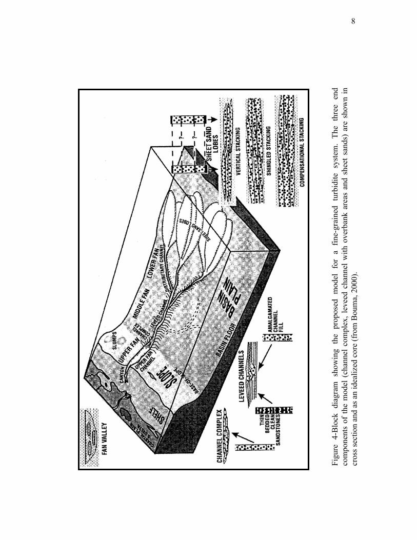
4 Block diagram showing the proposed model fora fine-grained turbidite system…………………………………………. 8
5 Schematic explanation of the deposition of sheet sands……………….. 10
6 Structure map of the top salt…………………………………………… 11
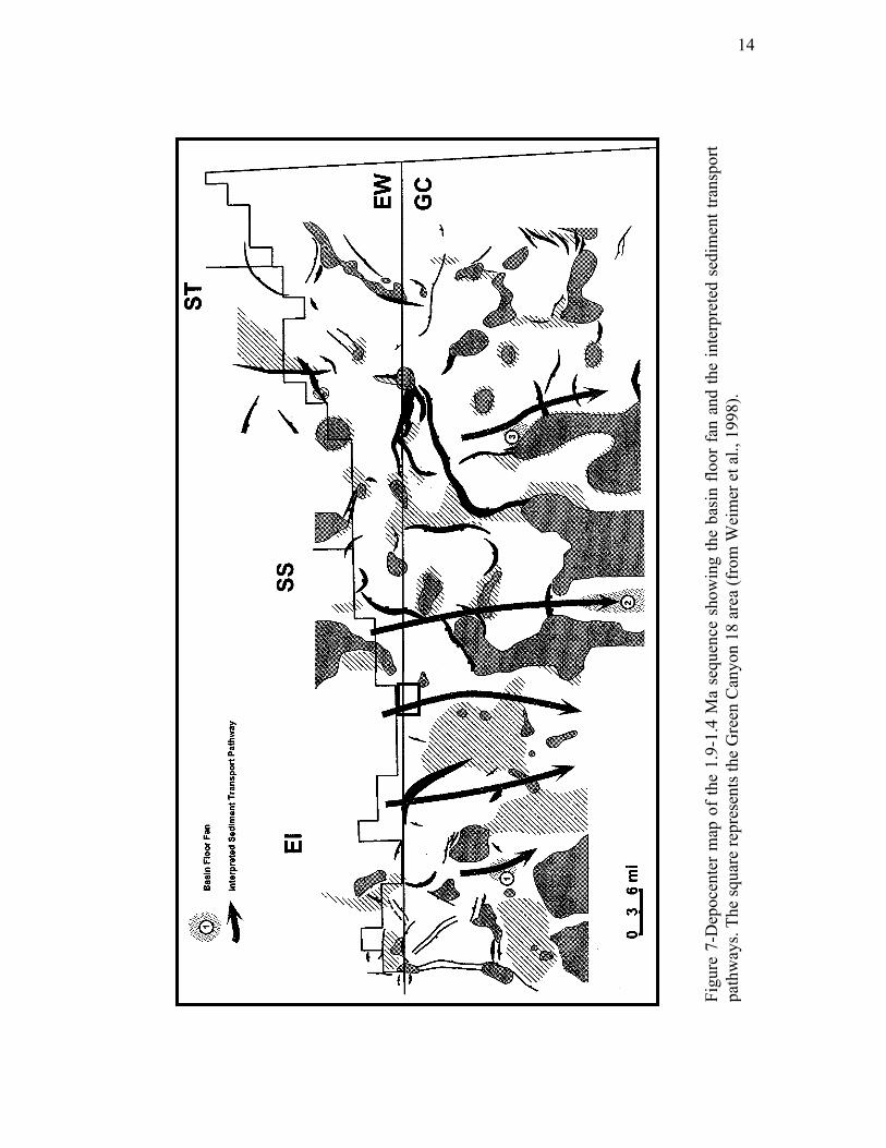
7 Depocenter map of the 1.9-1.4 Ma sequence showing the basinfloor fan and the interpreted sediment transport pathways…………….. 14
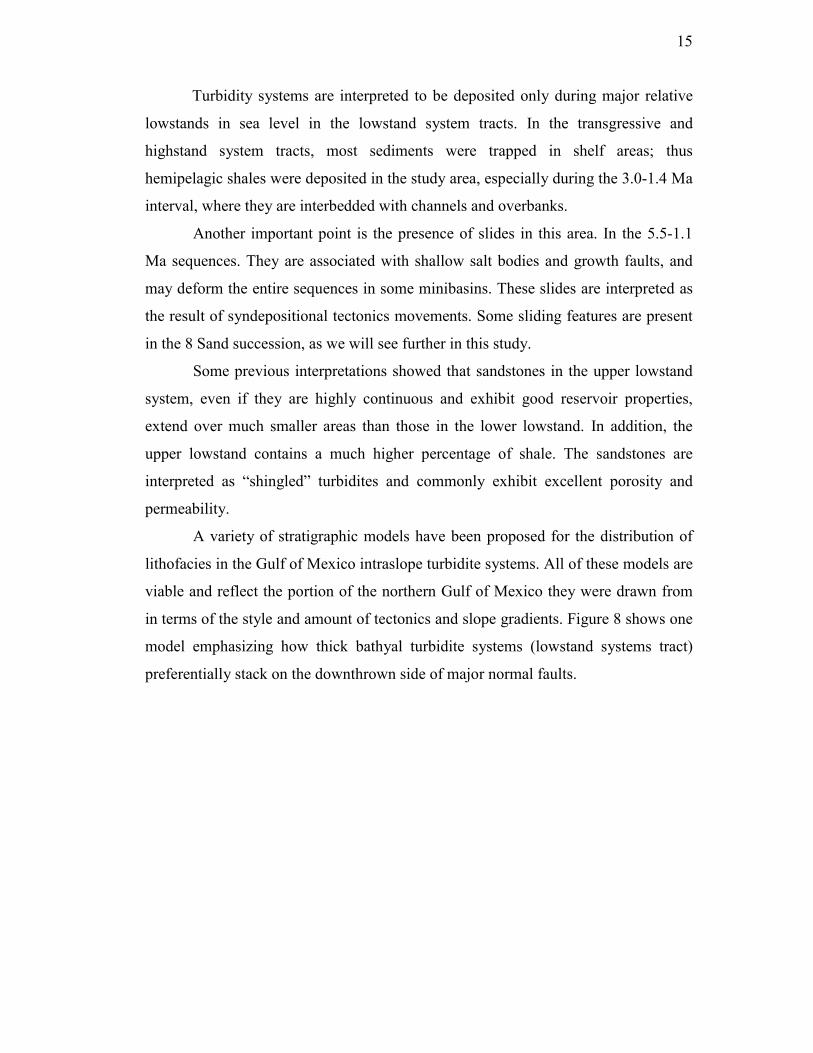
8 Depositional model for the northern Gulf of Mexicoshowing significant sands deposited on downthrownside of major expansion fault…………………………………………… 16
9 Log response of the 8 Sand interval at well A-2……………………….. 19
10 Log response of the 8 Sand interval at well A-25……………………… 20
11 Log response of the 8 Sand interval at well A-5……………………….. 20
12 Map showing the trajectory of the wells and the locationof the 8 sand intervals crossed by these wells………………………….. 22
13 Core picture showing an angular discordance caused bycore twisting in a facies E ……………………………………………… 24
14 Core picture showing alternating sand and shale layers in alevee deposit…………………………………………………………….. 25
ix
15 Core picture showing cross ripple lamination in a sand layer………….. 27
16 Core picture showing flame structures oriented from left to right…….. 28
17 Core picture showing flame structures oriented from right to left……… 28
18 Core picture showing a convolute bedding…………………………….. 30
19 Plot showing shaliness values computed from different methods……… 32
20 Comparison between minimum Vsh values from logs and…………….. 32Vsh values from cores
21 Shaliness-versus-Neutron-Density difference plot…………………….. 33
22 Correspondence between shaliness and Neutron-Density difference…… 35
23 Chart used for facies modelling ………………………………………... 36
24 Correlation between porosity values from cores and from logs………… 37
25 Plot showing petrophysical properties of facies A, C and E …………… 38
26 Diagram showing the depositional environment ofthe 8 Sand reservoir…………………………………………………….. 40
27 Map of the top of the 8 Sand reservoir………………………………….. 41
28 Gross thickness map……………………………………………………. 42
29 Correlation between half-energy time and reservoir thickness…………. 43
30 Net thickness map………………………………………………………. 44
31 Cross-section 1 from well correlation………………………………….. 46
32 Cross-section 2 from well correlation………………………………….. 47
33 Location of the three cross-sections……………………………………. 48
34 Cross-section 3 from well correlation………………………………….. 49
35 Reservoir model showing the facies repartition………………………… 51within the 8 Sand reservoir
x
LIST OF TABLES
TABLE Page
1 How to recognize the different facies from their log response………… 21
2 Standard deviation from core measurementsfor two different shaliness computation methods……………………… 33
3 8 Sand interval gross thickness, net thickness and net-to-gross ratio…... 34
4 Location of facies with associated porosity and permeability values…… 39
1
CHAPTER I
INTRODUCTION
Scope
Deep marine turbidite deposits are the focus of major exploration and
development efforts in the deep-water area of the Gulf of Mexico and worldwide. In
the United States, the Gulf of Mexico is now the primary area of exploration activity
for the major oil companies and these reservoirs are capable of world-class flow rates
and typically are massive and have large, well-connected areal extents.
This thesis attempts to characterize the main properties of the 8 Sand
reservoir in the Green Canyon 18 block, Gulf of Mexico, such as reservoir shape,
geological facies repartition and petrophysical properties. Ultimately this study will
help perform a reservoir simulation.
Objectives
The overall objective of this study is to increase knowledge of the geology of
the 8 Sand turbidite reservoir and to contribute to production strategy from this
reservoir. Specifically, this involves an integration of core and well log data to:
- Define and map the shape of the 8 Sand reservoir;
- Populate this body with facies and petrophysical properties;
- Provide some recommendations for a future reservoir simulation;
______________This thesis follows the style and format of the American Association of Petroleum GeologistsBulletin.
2
Location
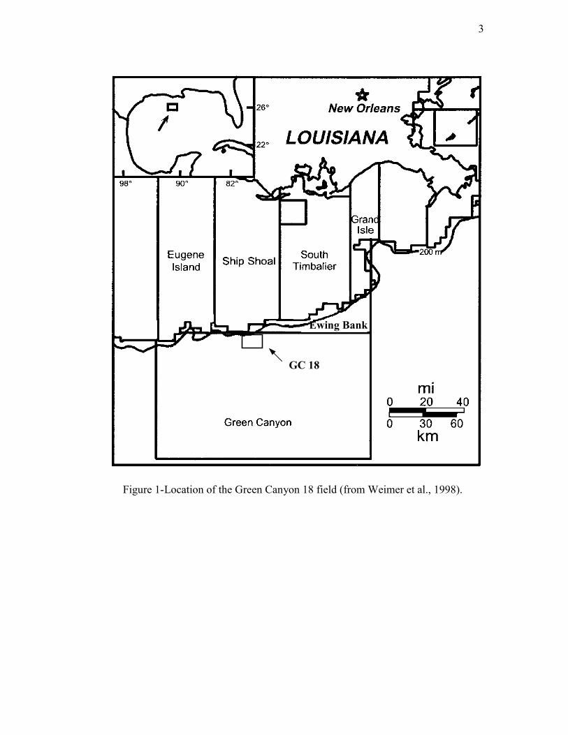
The Green Canyon Block 18 field is located 70 miles off of the Louisiana
coast (figure 1), south of Morgan City (Brinkmann et al., 1985).
Exxon/Mobil is the operator of Green Canyon 18 Field and has a 55%
working interest (WI). The other interest owners of the Green Canyon 18 Field are
BHP Petroleum (Americas) with a 25% WI, Burlington Resources with a 15% WI,
and Kerr-McGee Oil & Gas Corporation with a 5% WI. The development area is a
middle slope paleo-environment of Pliocene-Pleistocene age, which is in the
“Flexure” trend (Brinkmann et al., 1985). The discovery well, the Green Canyon 18
No.1, was drilled in December 1981 in 760 ft of water and reached a total depth of
13,127 ft MD in April 1982. Additional five exploration/appraisal wells were drilled
before the 30-slot platform was set in November 1986. Producing operations
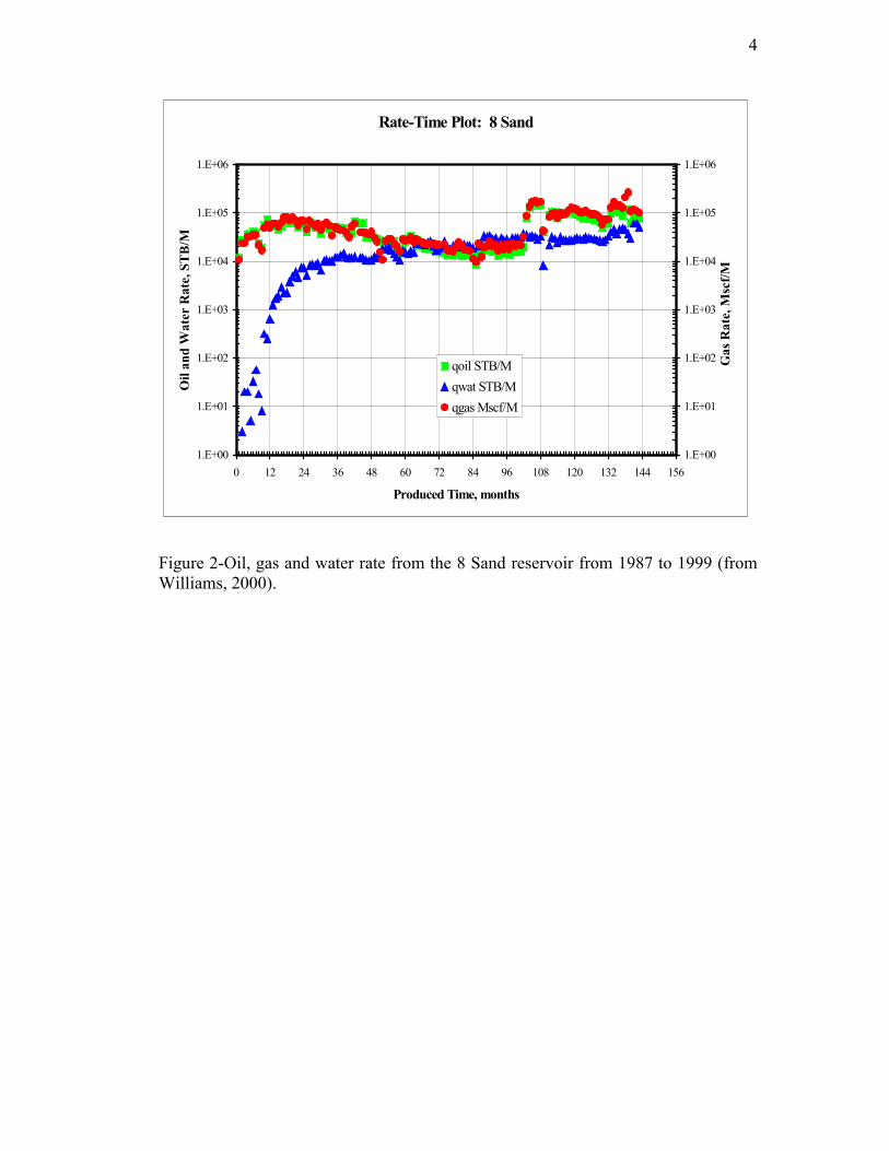
commenced in May 1987 (Ostermeier, 1993). Figure 2 shows a production plot for
the 8 Sand reservoir, which is the formation that we focused on. The monthly
production for the 8 Sand as of October 1999 was 78 MSTB of oil, which correspond
to a daily rate of 2,500 STB/D, and 102 MMscf of gas. Cumulative oil production
from the 8 Sand reservoir was 7 MMSTB of oil and 8 Bcf of gas in December 1999.
From these values, the original oil-in-place was estimated to be between 25 MMSTB
and 35 MMSTB of oil.
Data base
Data used for this study included well log measurements from 29 wells
throughout the Green Canyon 18 field, as well as core data that was provided by
Burlington Resources. Some previous reports about the production area were also
obtained courtesy of Burlington Resources. Lee Williams, who worked on the 8 Sand
reservoir for his thesis, also provided information about the 8 Sand reservoir.
3
Figure 1-Location of the Green Canyon 18 field (from Weimer et al., 1998).
GC 18
Ewing Bank
4
Figure 2-Oil, gas and water rate from the 8 Sand reservoir from 1987 to 1999 (fromWilliams, 2000).
Rate-Time Plot: 8 Sand
1.E+00
1.E+01
1.E+02
1.E+03
1.E+04
1.E+05
1.E+06
0 12 24 36 48 60 72 84 96 108 120 132 144 156
Produced Time, months
Oil
and
Wat
er R
ate,
ST
B/M
1.E+00
1.E+01
1.E+02
1.E+03
1.E+04
1.E+05
1.E+06
Gas
Rat
e, M
scf/M
qoil STB/Mqwat STB/Mqgas Mscf/M
5
CHAPTER II
BACKGROUND
Previous work on fine-grained turbidite deposits
Before dealing with the main characteristics of deepwater depositional
systems, it is important to focus on the exact terminology of the terms involved in the
description of these models. Deepwater depositional systems represent deposition
primarily by sediment gravity flows, which transport clastic sediment down a slope
and onto a basin floor (Stelting et al., 2000). These systems are called submarine fans
when referring to a modern deepwater accumulation exposed on the present-day sea
floor (Menard, 1955), or even in some cases to any unconsolidated sedimentary
succession. They are called turbidite systems when referring to subsurface and/or
outcrop occurrences (Mutti and Normark, 1987, 1991) and commonly to
consolidated deposits. Mutti and Normark (1991) define a turbidite (fan) system as “a
body of genetically related mass-flow and turbidity-current facies and facies
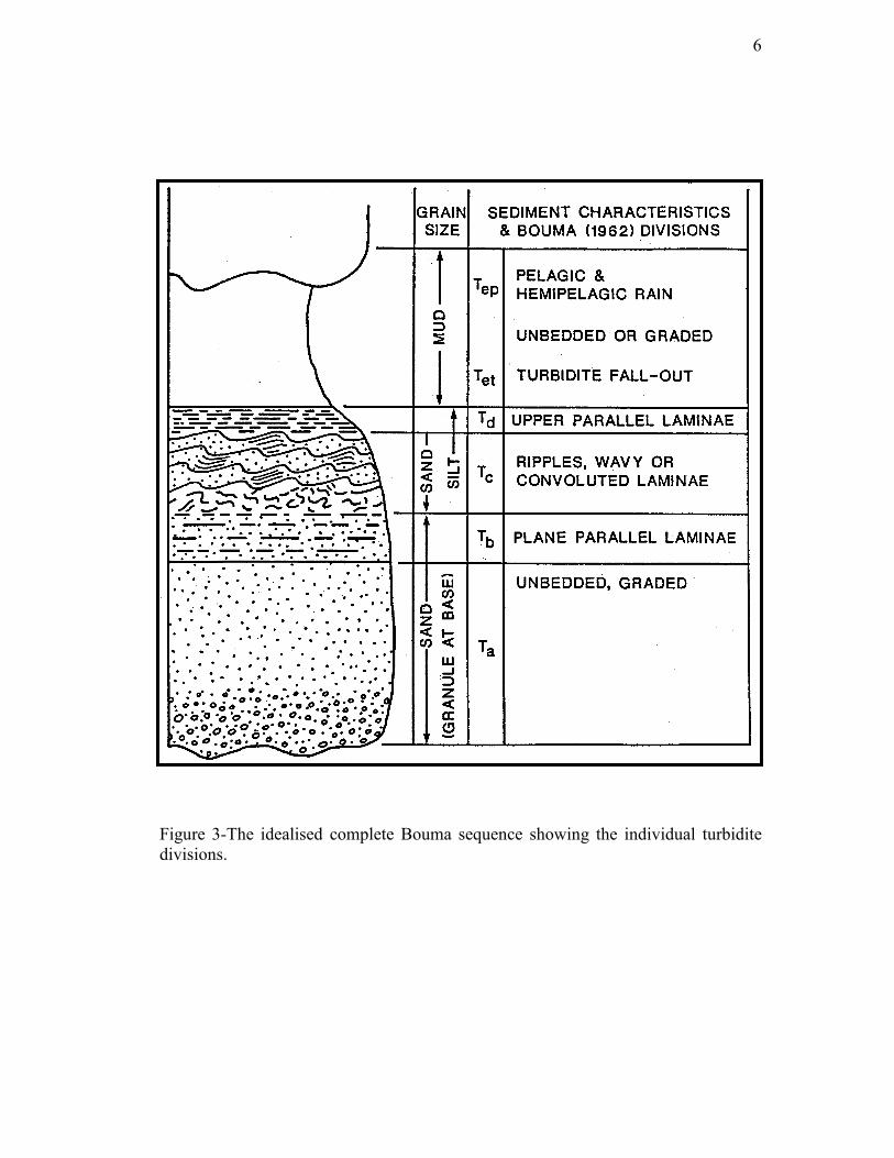
associations that were deposited in virtual stratigraphic continuity”. Bouma et al.
(1985a, b, c) called individual unconformity-bounded turbidite systems « fanlobes ».
Bouma created a sequence showing the ideal turbidite divisions (figure 3).
When stacked, turbidite (fan) systems and their bounding basinal shales are
defined as a turbidite (submarine fan) complex. If the shales or silty mudstones are
about the same thickness as the sand-rich beds of the individual turbidite systems or
if they comprise at least 70% of the total succession, the system is referred to as
being “mud-rich” (Reading and Richards, 1994). According to Stelting et al. (2000),
it is recommended to use turbidite system (complex) to refer to a composite
succession of sand and mud gravity flow deposits that form depositional units of
second-, third-, and/or fourth-order depositional sequences as defined by Posamontier
et al. (1988). Deepwater is also consistent for describing this kind of system.
6
Figure 3-The idealised complete Bouma sequence showing the individual turbiditedivisions.
7
Bouma et al. (1995a, b) proposed to divide a turbidite system into three main
parts: inner, mid- and outer zones. Three major parts can be identified with transition
zones in between. The base-of-slope, forming the transition from basin slope to basin
floor is characterized by a wide channel complex. The mid zone is comprised of a
leveed channel with extensive overbank deposits. The lower part of the midfan area
contains a transition made up by a distributary channel system. The outer zone is
characterized by sheet sands or depositional lobes (Bouma, 2000).
Turbidity flows do not flow continuously, even if fine material is likely to
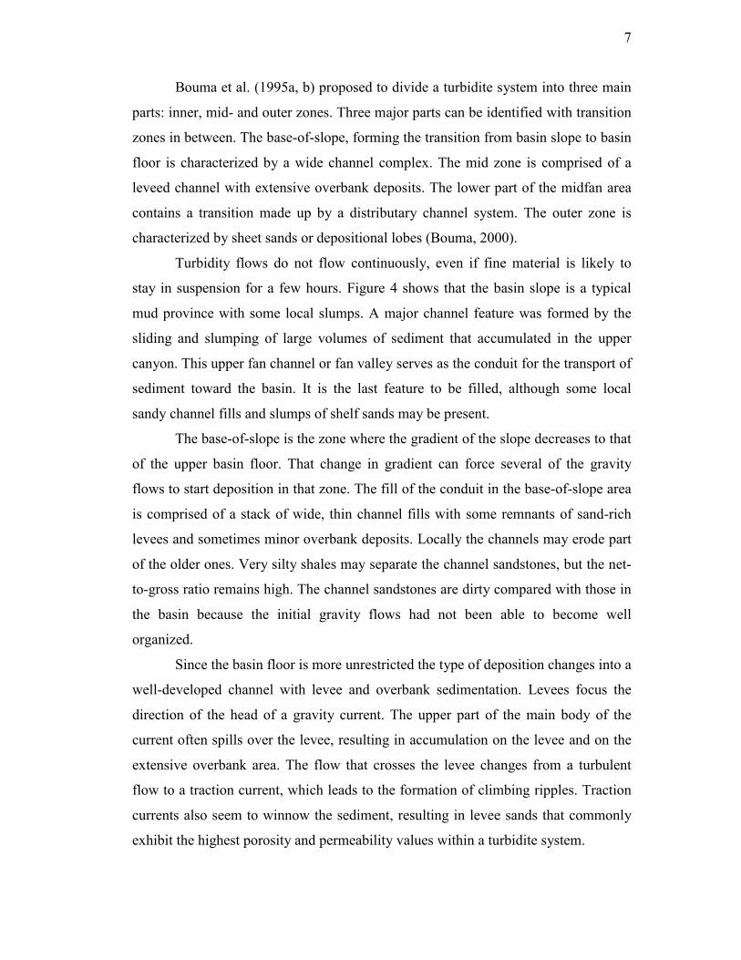
stay in suspension for a few hours. Figure 4 shows that the basin slope is a typical
mud province with some local slumps. A major channel feature was formed by the
sliding and slumping of large volumes of sediment that accumulated in the upper
canyon. This upper fan channel or fan valley serves as the conduit for the transport of
sediment toward the basin. It is the last feature to be filled, although some local
sandy channel fills and slumps of shelf sands may be present.
The base-of-slope is the zone where the gradient of the slope decreases to that
of the upper basin floor. That change in gradient can force several of the gravity
flows to start deposition in that zone. The fill of the conduit in the base-of-slope area
is comprised of a stack of wide, thin channel fills with some remnants of sand-rich
levees and sometimes minor overbank deposits. Locally the channels may erode part
of the older ones. Very silty shales may separate the channel sandstones, but the net-
to-gross ratio remains high. The channel sandstones are dirty compared with those in
the basin because the initial gravity flows had not been able to become well
organized.
Since the basin floor is more unrestricted the type of deposition changes into a
well-developed channel with levee and overbank sedimentation. Levees focus the
direction of the head of a gravity current. The upper part of the main body of the
current often spills over the levee, resulting in accumulation on the levee and on the
extensive overbank area. The flow that crosses the levee changes from a turbulent
flow to a traction current, which leads to the formation of climbing ripples. Traction
currents also seem to winnow the sediment, resulting in levee sands that commonly
exhibit the highest porosity and permeability values within a turbidite system.
8
Figu
re 4
-Blo
ck d
iagr
am s
how
ing
the
prop
osed
mod
el f
or a
fin
e-gr
aine
d tu
rbid
ite s
yste
m.
The
thre
e en
dco
mpo
nent
s of
the
mod
el (
chan
nel c
ompl
ex, l
evee
d ch
anne
l with
ove
rban
k ar
eas
and
shee
t san
ds)
are
show
n in
cros
s sec
tion
and
as a
n id
ealiz
ed c
ore
(fro
m B
oum
a, 2
000)
.
9
The channel fill commonly appears to be massive, being comprised of
amalgamated sandstones. The levees consist of alternating sandstones and shales.
The coarsest and the thickest levee sands can be expected closest to the channel
margin, whereas the mud-rich, lenticular-bedded sequences are found in the more
distal overbank sites. The sandstones usually contain foreset bedding, climbing
ripples, and parallel lamination. The sand-to-shale ratio can vary from 30 to 60%. It
can be noticed that the levees of the modern fan channels become progressively
smaller (i.e., thinner and less wide) down fan and finally disappear in the lower fan
area. The overbank deposits also have sandstone-shale couplets that gradually
become finer and thinner away from the channel, with a decreasing of the net-to-
gross ratio. The levee deposits are also known as low-resistivity, low-contrast, thin
bedded sandstones (Darling and Sneider, 1992). The individual layers are too thin to
detect on traditional electrical logs, although they can be excellent reservoirs because
of the high porosities and permeabilities (Bouma and Wickens, 1994).
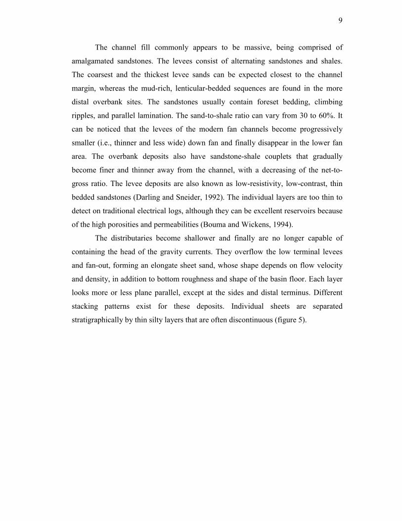
The distributaries become shallower and finally are no longer capable of
containing the head of the gravity currents. They overflow the low terminal levees
and fan-out, forming an elongate sheet sand, whose shape depends on flow velocity
and density, in addition to bottom roughness and shape of the basin floor. Each layer
looks more or less plane parallel, except at the sides and distal terminus. Different
stacking patterns exist for these deposits. Individual sheets are separated
stratigraphically by thin silty layers that are often discontinuous (figure 5).
10
Figure 5-Schematic explanation of the deposition of sheet sands. (A) A succession ofindividual sandstone layers. Note the amalgamated (or very thin shale) contactbetween the centers of the slightly convexed-shaped sandstones. (B) Two packagesof sandstones onlap onto each other. These packages are called sheet sands.Individual sandstones may be 10-80 cm thick; a package can range in width from 500to more than 1000 m.
Geological setting
A major interest in the Gulf of Mexico is the complex relationship between
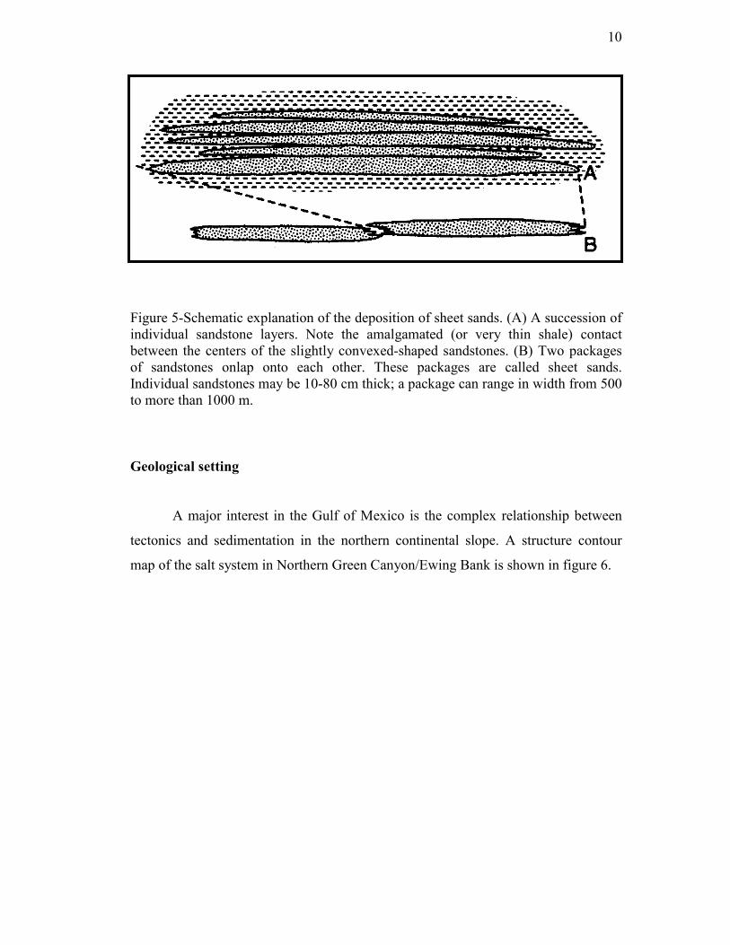
tectonics and sedimentation in the northern continental slope. A structure contour
map of the salt system in Northern Green Canyon/Ewing Bank is shown in figure 6.
11
Figure 6-Structure map of the top salt (from Weimer et al., 1998). The black squarerepresents the Green Canyon 18 area.
The most prominent feature of this salt system is its large relief, with the tops
of the shallowest diapers at less than 1.0 s two-way traveltime and the deepest salt
welds at more than 7.5 s two-way traveltime. The pattern is a complex one in which
different salt bodies have evolved and amalgamated through time to create a
composite salt system with multiple levels. Diapirs generally are found along the
frontal or lateral edges of shallow sheets. These diapers usually do not have deep
roots and have variable geometries. In plan view, they range from circular to highly
irregular. To the north, the salt system is dominated by the southern portions of
shallow sheets that extend to the north onto the shelf. These northern areas generally
have thin remnant salt between scattered small diapers with no deep roots, and the
diapirs along the southern edges of the sheets commonly have been modified by
contractional squeezing. To the south, salt bodies usually are thicker and of larger
areal extent, with roots that connect them to the underlying ridges and saddles in the
base-salt surface (Weimer et al., 1998).
The different types of salt systems impact the stratigraphic evolution of the
minibasins of this area in several ways. First, these salt systems determine the
12
shifting location and shape of minibasins through time. Second, they define the local
sea-floor paleobathymetry during each depositional cycle, and also dictate
subsequent basin modification (thereby producing structural traps). Third, the
evolution of each type of system determines whether there is adequate underlying
salt to provide accommodation for vertical stacking of ponded sands. Thus salt
tectonics has a major influence on the geometry of the turbidite reservoirs by
impacting the deposition environment of the turbidity currents.
The productive strata in the Green Canyon Block 18 Field occur within a
single sequence. The primary reservoirs of Green Canyon 18 are part of a mounded
turbidite package that was deposited by density grain flows and debris flows with
possible reworking by bottom-hugging, deep water (contourite) currents along the
north flank of the Green Canyon salt dome. The main reservoir target sands of Block
18 occur in the bend of the channel complex, on this northern flank. These sands are
part of a northwest-southeast trending anticline that is bounded on the south by a
southeast dipping extensional fault.
Seismic and geologic facies change abruptly across the area in all sequences,
reflecting the lateral and vertical changes in lithofacies from sand-rich to mud-rich
systems (Weimer, 1998). The lower reservoirs (e.g., 20, 26 and 30 Sands) are coarser
grained and more massive than the shallower reservoirs, which tend to be highly
laminated. These sandstones were deposited during the Upper Pliocene and Lower
Pleistocene. The Upper Pliocene 8 Sand is in the upper lowstand sequence, within the
1.9-1.4 Ma sequence, also called “CM” sequence. Biostratigraphic data suggest that
this sequence is a fourth order sequence. It has been demonstrated that there are
spatial and temporal variations of the turbidite deposits throughout the Green Canyon
area.
Sheet sands (depositional lobes or basin-floor fans) seem to represent only a
minor portion of the sequences in terms of thickness and areal distribution (Weimer
et al., 1998). In the 3.0-0.7 Ma sequences, the basin-floor fans do not fill minibasins,
unlike the older ones, so their areal extent is less. These kinds of fans were deposited
in the downthrown side of growth faults and adjacent to shallow salt bodies in lower
bathyal water depths. The tectonic elements helped to create localized bathymetric
lows on the sea floor, and the lobes were deposited in these restricted areas. But lobe
13
fans are not likely to be present during the 1.9-1.4 Ma sequence in the Green Canyon
18 area as we can see in figure 7. The study area was located much closer to the
shelf.
One proposed interpretation is that this period was more influenced by faults
than by salt tectonics, and that the active large salt withdrawal basins were more
effective in trapping coarse-grained sediments than the fault-related basins. Perhaps
the abrupt changes in bathymetric relief that caused sand deposition from turbidity
currents were greater in these salt-withdrawal basins (Weimer et al., 1998). It could
also been related to the increase in clay in turbidity current delivered to the basin.
Concerning the channel-levee systems, it appears that the number and sand
content of the channel systems gradually decreased through time throughout the area.
Thus channel fills are not common in the 1.9-1.4 Ma sequence, maybe because the
large unchannelized flows of mud-rich sediments have become more dominant in the
more shaly Pleistocene sequences.
Due to this decrease in channel systems, the overbank deposits, interpreted as
mostly shales interbedded with silty sands, are interpreted as large unchannelized
flows of mud-rich sediments transported into the area.
14
Figu
re 7
-Dep
ocen
ter m
ap o
f the
1.9
-1.4
Ma
sequ
ence
sho
win
g th
e ba
sin
floor
fan
and
the
inte
rpre
ted
sedi
men
t tra
nspo
rtpa
thw
ays.
The
squa
re re
pres
ents
the
Gre
en C
anyo
n 18
are
a (f
rom
Wei
mer
et a
l., 1
998)
.
15
Turbidity systems are interpreted to be deposited only during major relative
lowstands in sea level in the lowstand system tracts. In the transgressive and
highstand system tracts, most sediments were trapped in shelf areas; thus
hemipelagic shales were deposited in the study area, especially during the 3.0-1.4 Ma
interval, where they are interbedded with channels and overbanks.
Another important point is the presence of slides in this area. In the 5.5-1.1
Ma sequences. They are associated with shallow salt bodies and growth faults, and
may deform the entire sequences in some minibasins. These slides are interpreted as
the result of syndepositional tectonics movements. Some sliding features are present
in the 8 Sand succession, as we will see further in this study.
Some previous interpretations showed that sandstones in the upper lowstand
system, even if they are highly continuous and exhibit good reservoir properties,
extend over much smaller areas than those in the lower lowstand. In addition, the
upper lowstand contains a much higher percentage of shale. The sandstones are
interpreted as “shingled” turbidites and commonly exhibit excellent porosity and
permeability.
A variety of stratigraphic models have been proposed for the distribution of
lithofacies in the Gulf of Mexico intraslope turbidite systems. All of these models are
viable and reflect the portion of the northern Gulf of Mexico they were drawn from
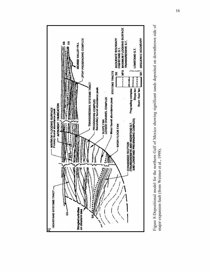
in terms of the style and amount of tectonics and slope gradients. Figure 8 shows one
model emphasizing how thick bathyal turbidite systems (lowstand systems tract)
preferentially stack on the downthrown side of major normal faults.
16
Figu
re 8
-Dep
ositi
onal
mod
el fo
r the
nor
ther
n G
ulf o
f Mex
ico
show
ing
sign
ifica
nt s
ands
dep
osite
d on
dow
nthr
own
side
of
maj
or e
xpan
sion
faul
t (fr
om W
eim
er e
t al.,
199
8).
17
CHAPTER III
METHODS
Data overview
All the data have been provided by Burlington and consist mainly of binders
that contain geological, geophysical and production information. Associated to these
hard data were furnished digital tapes with 3D seismic and well log data recorded
throughout the Green Canyon 18 field.
The well log data concerned more than 30 wells and most of the time
comprised all the “classical” measurement such as Gamma-Ray, Caliper,
Spontaneous Potential, Spherically Focused laterolog, Medium and Deep Induction
Tool, Sonic, Compensated Neutron Log and Formation Density Log. Unfortunately,
sometimes only Gamma Ray measurement was provided. A second set of well log
data was composed of already interpreted logs such as porosity, shaliness (Vsh) and
water saturation logs.
Associated to these log data were provided core measurements that had been
performed in several wells in the Green Canyon 18 field. These core analysis were
performed by Petroleum Testing Service, Inc., Houston, Texas, and gave information
about porosity, permeability, oil and water saturation, apparent sand grain density
and lithology of the 8 Sand reservoir.
There were some limitations in the using of these data. First it was soon clear
that only a little part of the cores were taken in the 8 Sand interval. Secondly the
porosity core values were not likely to represent those within the reservoir, since the
pressure conditions were obviously not the same. It was difficult to determine the
order of magnitude of discrepancies between these values because different
mechanisms are involved, such as rock and fluid compressibility, or fluid pressure
that counterbalance the lithostatic pressure inside the reservoir. Nevertheless, some
authors assumed that conventional and sidewall core data read lower than in-situ

18
porosity because of what they call the “snowball effect” (Dunham, 1995). Thus these
values have to be carefully examined before being used. Another limitation
concerned the fluid saturation of the rock samples. Since the total fluid saturation
never reached 100% in all the cores, only the oil/water ratio was likely to give
relevant information about the volumes of hydrocarbons present in the reservoir.
Thus we extracted saturation values from previous studies on 8 Sand reservoir.
Location of the 8 Sand intervals
The first step of the study consisted in locating the 8 Sand intervals in the
wells. Former studies had been already performed, showing the depth of the 8 Sand
intervals in 16 wells. We checked if these figures were adequate and tried to look for
other wells crossing the 8 Sand formation. The main difficulty consisted in the log
response of the 8 Sand that is not homogeneous throughout the field. In some wells
the log response was very close to the shale response. Figures 9, 10 and 11 show
three examples of 8 Sand log responses.
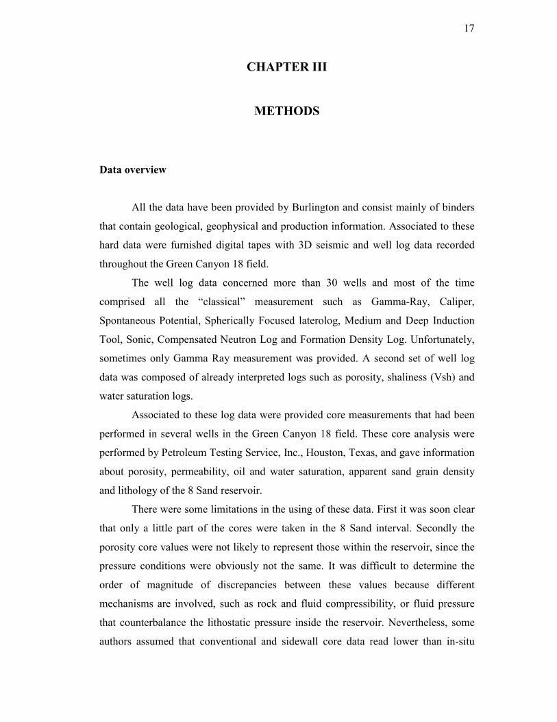
In well A-2, a 9-feet thick interval between 10900 and 10909 ft MD was
assumed to be a channel fill deposit. Indeed the Gamma Ray value is quite low
compare to the surrounding facies, the resistivity values are high and the Neutron-
Density difference revealed a massive sand signature. Below there is also a 2-feet
thick sandy interval that could represent the lateral extremity of another channel. We
also noticed that a 4-feet thick shale layer, which could give some information about
connectivity between stacked channels, separated these two sandy levels. The rest of
the interval is composed of levee and overbank deposits, with high Gamma Ray, low
resistivity and Neutron-Density difference close to the one of shale (Low-Resistivity
Sand response). No core data were available for this well.
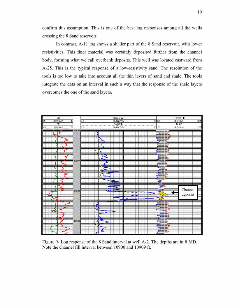
In well A-25, the base of the reservoir between 9960 and 9990 ft MD is very
sandy, even if the rapid variations of the shallow resistivity tool are in favor of
laminated facies. Two small intervals seem to be channel deposits, for the same
reasons as in the previous well. The very high permeability vales in this zone tend to
19
confirm this assumption. This is one of the best log responses among all the wells
crossing the 8 Sand reservoir.
In contrast, A-11 log shows a shalier part of the 8 Sand reservoir, with lower
resistivities. This finer material was certainly deposited further from the channel
body, forming what we call overbank deposits. This well was located eastward from
A-25. This is the typical response of a low-resistivity sand. The resolution of the
tools is too low to take into account all the thin layers of sand and shale. The tools
integrate the data on an interval in such a way that the response of the shale layers
overcomes the one of the sand layers.
Figure 9- Log response of the 8 Sand interval at well A-2. The depths are in ft MD.Note the channel fill interval between 10900 and 10909 ft.
Channeldeposits
20
Figure 10-Log response of the 8 Sand interval at well A-25. The depths are in ft MD.
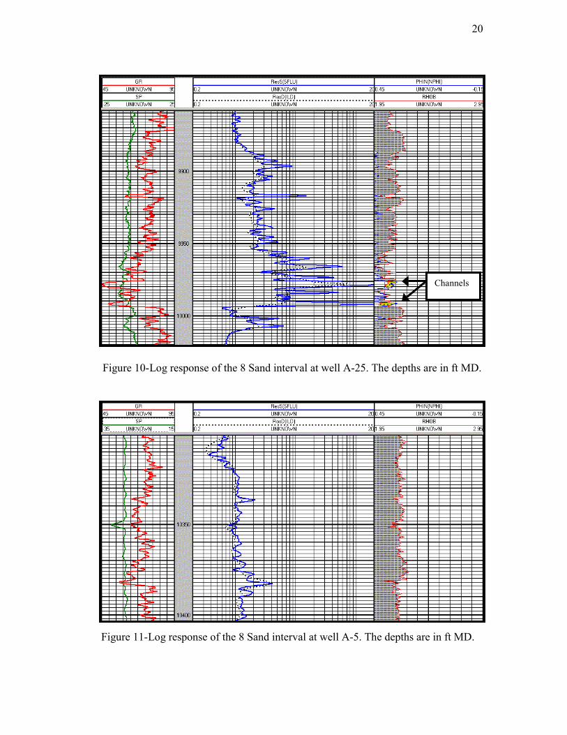
Figure 11-Log response of the 8 Sand interval at well A-5. The depths are in ft MD.
Channels
21
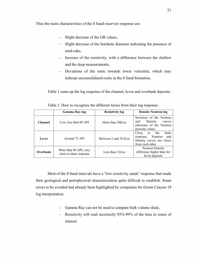
Thus the main characteristics of the 8 Sand reservoir response are:
- Slight decrease of the GR values,
- Slight decrease of the borehole diameter indicating the presence of
mud-cake,
- Increase of the resistivity, with a difference between the shallow
and the deep measurements,
- Deviations of the sonic towards lower velocities, which may
indicate unconsolidated rocks in the 8 Sand formation.
Table 1 sums up the log response of the channel, levee and overbank deposits.
Table 1. How to recognize the different facies from their log response.Gamma-Ray log Resistivity log Density-Neutron log
Channel Low, less than 60 API More than 20�.mInversion of the Neutronand Density curves(decrease of the Neutronporosity value)
Levee Around 75 API Between 2 and 10 �.m
Close to the shaleresponse, Neutron andDensity curves are closerfrom each other
Overbank More than 80 API, veryclose to shale response Less than 2 �.m
Neutron-Densitydifference higher than for
levee deposits
Most of the 8 Sand intervals have a “low resistivity sands” response that made
their geological and petrophysical characterization quite difficult to establish. Some
errors to be avoided had already been highlighted by companies for Green Canyon 18
log interpretation:
- Gamma Ray can not be used to compute bulk volume shale,
- Resistivity will read incorrectly 95%-99% of the time in zones of
interest.
22
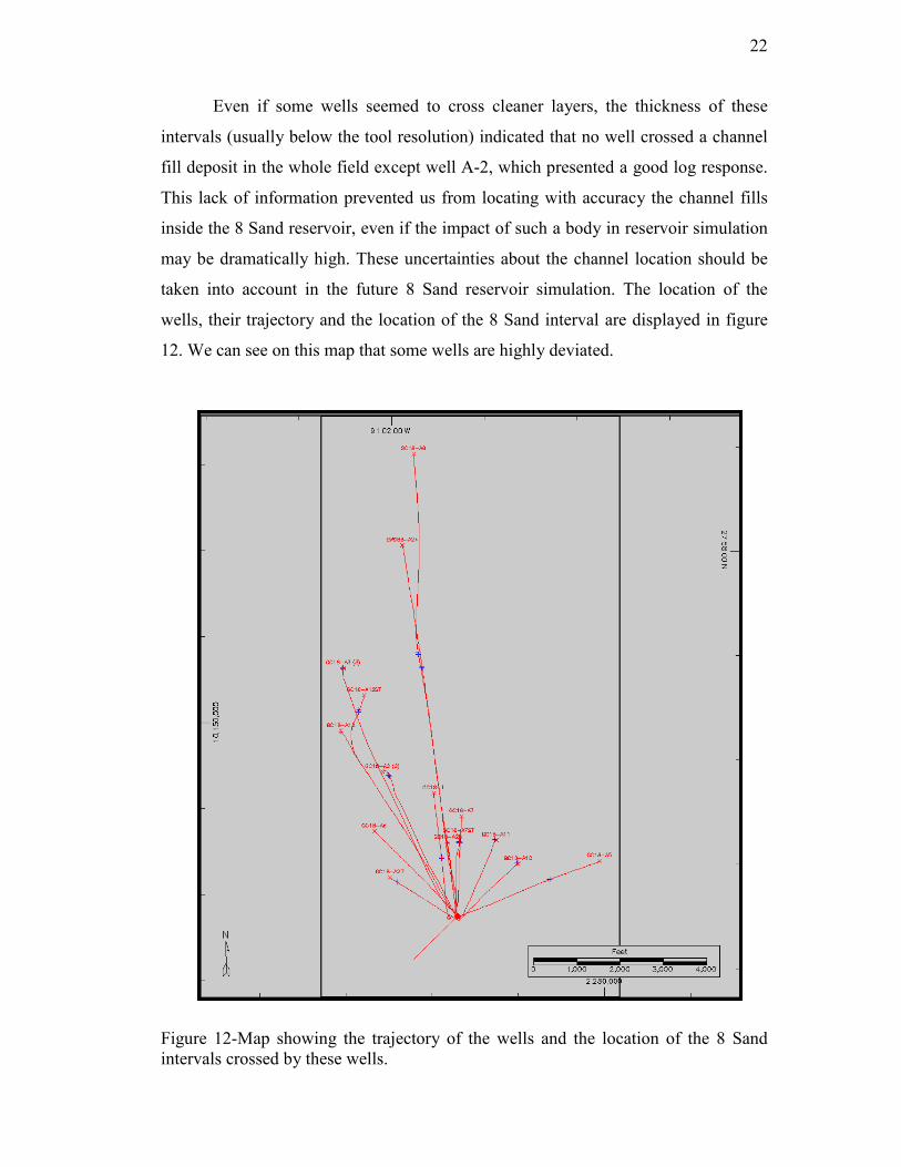
Even if some wells seemed to cross cleaner layers, the thickness of these
intervals (usually below the tool resolution) indicated that no well crossed a channel
fill deposit in the whole field except well A-2, which presented a good log response.
This lack of information prevented us from locating with accuracy the channel fills
inside the 8 Sand reservoir, even if the impact of such a body in reservoir simulation
may be dramatically high. These uncertainties about the channel location should be
taken into account in the future 8 Sand reservoir simulation. The location of the
wells, their trajectory and the location of the 8 Sand interval are displayed in figure
12. We can see on this map that some wells are highly deviated.
Figure 12-Map showing the trajectory of the wells and the location of the 8 Sandintervals crossed by these wells.
23
Sedimentary analysis of the 8 Sand formation
This sedimentary study was only based on one set of core pictures from well
A-7. These pictures represent conventional-well cores (4 inches) coming from the
Green Canyon 18 area. They were examined in order to describe some sedimentary
features, determine the principal sedimentary facies, determine environments of
deposition and, if possible, relate sedimentary facies to reservoir quality. The
described interval was comprised between 9961 ft and 10050 ft. Since most of the
wells are deviated in this field, the depths noted are the measured depths, and not
corrected “true vertical depths”. Coring was not continuous through this interval.
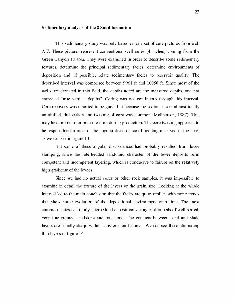
Core recovery was reported to be good, but because the sediment was almost totally
unlithified, dislocation and twisting of core was common (McPherson, 1987). This
may be a problem for pressure drop during production. The core twisting appeared to
be responsible for most of the angular discordance of bedding observed in the core,
as we can see in figure 13.
But some of these angular discordances had probably resulted from levee
slumping, since the interbedded sand/mud character of the levee deposits form
competent and incompetent layering, which is conducive to failure on the relatively
high gradients of the levees.
Since we had no actual cores or other rock samples, it was impossible to
examine in detail the texture of the layers or the grain size. Looking at the whole
interval led to the main conclusion that the facies are quite similar, with some trends
that show some evolution of the depositional environment with time. The most
common facies is a thinly interbedded deposit consisting of thin beds of well-sorted,
very fine-grained sandstone and mudstone. The contacts between sand and shale
layers are usually sharp, without any erosion features. We can see these alternating
thin layers in figure 14.
24
Figure 13-Core picture showing an angular discordance caused by core twisting in afacies E. This core comes from well A-7, at a depth of 9994 ft MD.
0.5 ft
25
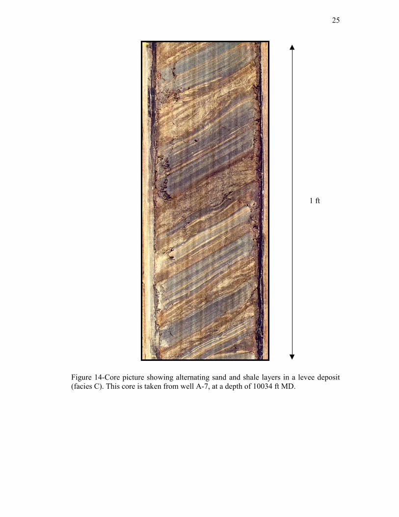
Figure 14-Core picture showing alternating sand and shale layers in a levee deposit(facies C). This core is taken from well A-7, at a depth of 10034 ft MD.
1 ft
26
This facies displays various types of lenticular, wavy, and flaser bedding.
Distinction between these types is based on the sandstone-to-mudstone ratio
(Reineck and Singh, 1973). The individual sand layers show a thickness range of 0.1-
3 inches, although locally sand beds up to one foot thick are present. We interpreted
these thickness variations as an indicator of the position of the deposit with respect to
the channel location. The sand content was computed by measuring the thickness of
the sandstone and mudstone layers, and was mostly in the range of 30-70%. In some
cores we could detect some fining-upward trends.
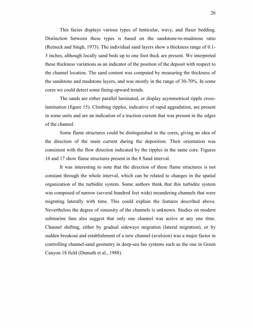
The sands are either parallel laminated, or display asymmetrical ripple cross-
lamination (figure 15). Climbing ripples, indicative of rapid aggradation, are present
in some units and are an indication of a traction current that was present in the edges
of the channel.
Some flame structures could be distinguished in the cores, giving an idea of
the direction of the main current during the deposition. Their orientation was
consistent with the flow direction indicated by the ripples in the same core. Figures
16 and 17 show flame structures present in the 8 Sand interval.
It was interesting to note that the direction of these flame structures is not
constant through the whole interval, which can be related to changes in the spatial
organization of the turbidite system. Some authors think that this turbidite system
was composed of narrow (several hundred feet wide) meandering channels that were
migrating laterally with time. This could explain the features described above.
Nevertheless the degree of sinuosity of the channels is unknown. Studies on modern
submarine fans also suggest that only one channel was active at any one time.
Channel shifting, either by gradual sideways migration (lateral migration), or by
sudden breakout and establishment of a new channel (avulsion) was a major factor in
controlling channel-sand geometry in deep-sea fan systems such as the one in Green
Canyon 18 field (Damuth et al., 1988).
27
Figure 15-Core picture showing cross ripple lamination in a sand layer. Therelatively coarser sand is indicative of a deposit close to a turbidite channel. This corewas taken from well A-7, at a depth of 10036 ft MD.
0.5 ft

28
Figure 16-Core picture showing flame structures oriented from left to right. This corewas taken from well A-7, at a depth of 10027 ft MD.
Figure 17-Core picture showing flame structures oriented from right to left. This corewas taken from well A-7, at a depth of 10011 ft MD.
0.5 ft
0.1 ft
29
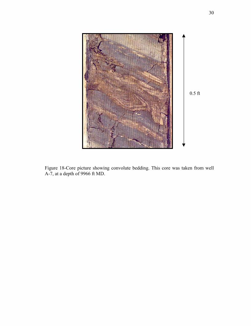
Convolute bedding and small-scale loading structures were also present in
some cores (figure 18). These structures point to conditions of rapid deposition
(Brenchley and Newall, 1977). Some portions of the cores contained more mudstone
facies, indicating a deposition further from the channel.
All these remarks were consistent with a turbidite interpretation. These
bedded facies could be interpreted to be deposits of relatively fine-grained sediment
from both traction and suspension modes.
Because the thickness of the larger sand layer did not exceed 2 feet, we
concluded that no channel-fill deposits were visible on these core pictures, even if at
some locations of the interval the deposits are likely to be adjacent to a channel. We
also inferred that the vertical permeability inside the reservoir should be very low,
regarding the laminated nature of the deposits. Thus the kv/kh ratio used in the
reservoir simulation should be very low. It is important to note that sedimentary
features such as ripples or convolutes are likely to interfere with fluid circulation
because they create a preferential path for the fluids in motion. Sometimes the
contact between channel and levee facies is interpreted as a barrier to fluid flow
because there may be a shale interface between the two facies. We did not have any
information about the lateral extent of the shale layers, but it is usually admitted that
levee and overbank deposits are likely to present good lateral continuity.
Reservoir quality in the Green Canyon 18 field seems to be controlled mainly
by permeability. In general, reservoir quality in the sands is high, with porosities
around 35% and permeabilities, which can reach 3300 mD. One of the main features
in Green canyon 18 cores is that the sediments are unconsolidated because diagenetic
modification of depositional porosity and permeability is minimal (Beard and Weyl,
1973). Thus reservoir quality is principally controlled by depositional facies.
30
Figure 18-Core picture showing convolute bedding. This core was taken from wellA-7, at a depth of 9966 ft MD.
0.5 ft

31
Management of porosity values
8 Sand porosity values derived from cores were only available on six wells in
the Green Canyon 18 field. These wells were A-25, A-12, A-7, A-8, A-11 and A-27.
Most of the data concerned wells A-7 and A-12.
All the porosity values are high in the 8 Sand reservoir. In this kind of
deposits, the high porosities at these depths are attributed to combined effects of
excellent grain sorting, high pore pressure, and minimal cementation (Reedy and
Pepper, 1996).
Computation of the net thickness
One of the main objectives of this study was to determine the net thickness of
the 8 Sand formation. The main parameter that we had to deal with was the shaliness
(Vsh). Shaliness is usually computed from log data thanks to different tools: Gamma
Ray, spontaneous potential and Neutron-Density. We could not use the Gamma Ray
method because of the high-Gamma Ray response of the 8 Sand: we would have
overestimated the shaliness value. Thus we tried to compute it with the two other
methods.
In parallel we decided to use the core pictures in the purpose of measuring the
amount of shale and sand in the cores. In this objective, we measured the thickness of
the sand and shale layers, and converted these values into percentages. Even though
the precision of measurements was not absolute we could obtain a good
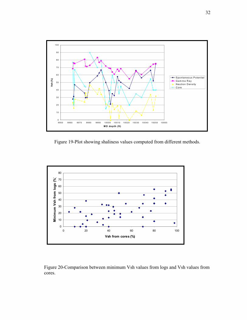
approximation of the reality. Then we tried to fit these values with the ones
calculated from logs. Unfortunately, due to the bad resolution of the tools, the results
were not really consistent. Some shaliness values from previous studies, based on
core measurement, were also available, and were used as reference values. Many
discrepancies exist between the log values and the measured values, as illustrated in
figures 19 and 20. We could not find the evidence of a correlation between the
different wells. Table 2 shows the standard deviation between the core values and the
computed values from the Gamma Ray and the Spontaneous Potential tools.
32
Figure 19-Plot showing shaliness values computed from different methods.
Figure 20-Comparison between minimum Vsh values from logs and Vsh values fromcores.
0
10
20
30
40
50
60
70
80
90
100
9950 9960 9970 9980 9990 10000 10010 10020 10030 10040 10050 10060
M D de p th (ft)
Vsh
(%) S po ntan eo u s P o ten tia l
G a m m a R a yN eu tro n D en sityC ore
0
10
20
30
40
50
60
70
80
0 20 40 60 80 100
Vsh from cores (%)
Min
imum
Vsh
from
logs
(%)
33
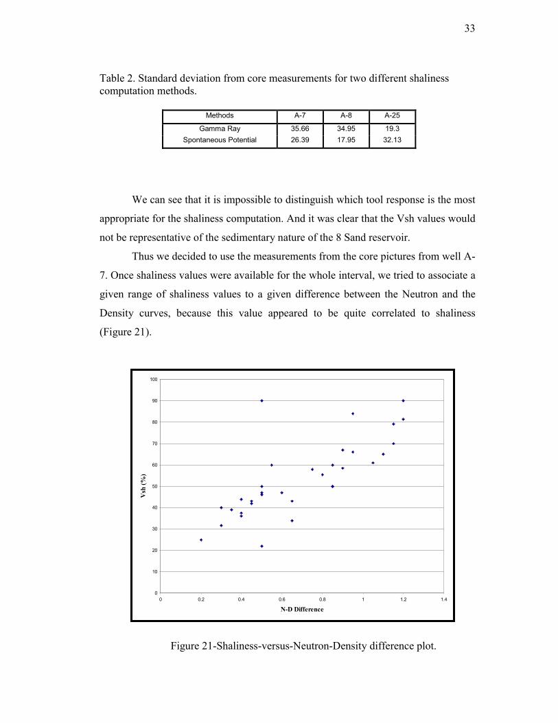
Table 2. Standard deviation from core measurements for two different shalinesscomputation methods.
Methods A-7 A-8 A-25
Gamma Ray 35.66 34.95 19.3Spontaneous Potential 26.39 17.95 32.13
We can see that it is impossible to distinguish which tool response is the most
appropriate for the shaliness computation. And it was clear that the Vsh values would
not be representative of the sedimentary nature of the 8 Sand reservoir.
Thus we decided to use the measurements from the core pictures from well A-
7. Once shaliness values were available for the whole interval, we tried to associate a
given range of shaliness values to a given difference between the Neutron and the
Density curves, because this value appeared to be quite correlated to shaliness
(Figure 21).
Figure 21-Shaliness-versus-Neutron-Density difference plot.
0
10
20
30
40
50
60
70
80
90
100
0 0.2 0.4 0.6 0.8 1 1.2 1.4
N-D Difference
Vsh
(%)
34
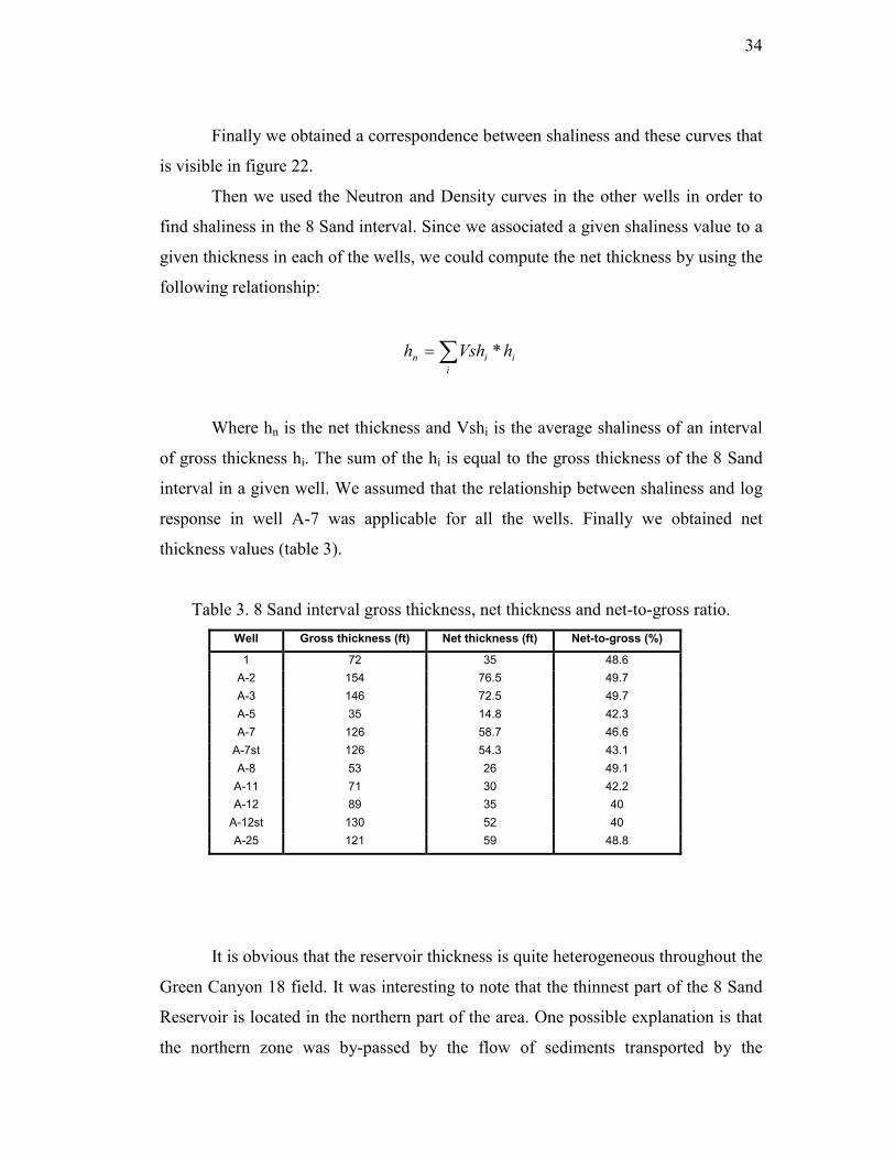
Finally we obtained a correspondence between shaliness and these curves that
is visible in figure 22.
Then we used the Neutron and Density curves in the other wells in order to
find shaliness in the 8 Sand interval. Since we associated a given shaliness value to a
given thickness in each of the wells, we could compute the net thickness by using the
following relationship:
��i
iin hVshh *
Where hn is the net thickness and Vshi is the average shaliness of an interval
of gross thickness hi. The sum of the hi is equal to the gross thickness of the 8 Sand
interval in a given well. We assumed that the relationship between shaliness and log
response in well A-7 was applicable for all the wells. Finally we obtained net
thickness values (table 3).
Table 3. 8 Sand interval gross thickness, net thickness and net-to-gross ratio.Well Gross thickness (ft) Net thickness (ft) Net-to-gross (%)
1 72 35 48.6A-2 154 76.5 49.7A-3 146 72.5 49.7A-5 35 14.8 42.3A-7 126 58.7 46.6
A-7st 126 54.3 43.1A-8 53 26 49.1
A-11 71 30 42.2A-12 89 35 40
A-12st 130 52 40A-25 121 59 48.8
It is obvious that the reservoir thickness is quite heterogeneous throughout the
Green Canyon 18 field. It was interesting to note that the thinnest part of the 8 Sand
Reservoir is located in the northern part of the area. One possible explanation is that
the northern zone was by-passed by the flow of sediments transported by the
35
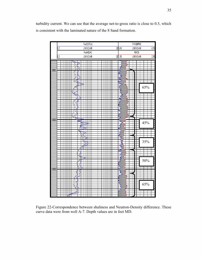
turbidity current. We can see that the average net-to-gross ratio is close to 0.5, which
is consistent with the laminated nature of the 8 Sand formation.
Figure 22-Correspondence between shaliness and Neutron-Density difference. Thesecurve data were from well A-7. Depth values are in feet MD.
65%
45%
35%
50%
65%
36
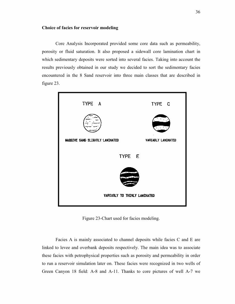
Choice of facies for reservoir modeling
Core Analysis Incorporated provided some core data such as permeability,
porosity or fluid saturation. It also proposed a sidewall core lamination chart in
which sedimentary deposits were sorted into several facies. Taking into account the
results previously obtained in our study we decided to sort the sedimentary facies
encountered in the 8 Sand reservoir into three main classes that are described in
figure 23.
Figure 23-Chart used for facies modeling.
Facies A is mainly associated to channel deposits while facies C and E are
linked to levee and overbank deposits respectively. The main idea was to associate
these facies with petrophysical properties such as porosity and permeability in order
to run a reservoir simulation later on. These facies were recognized in two wells of
Green Canyon 18 field: A-8 and A-11. Thanks to core pictures of well A-7 we
37
managed to describe these facies in this well. Then we tried to locate these facies in
all the wells thanks to the criteria described in the previous sections. Once all the
well intervals were populated with facies, we decided to associate each interval with
porosity and permeability values.
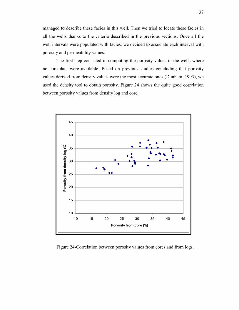
The first step consisted in computing the porosity values in the wells where
no core data were available. Based on previous studies concluding that porosity
values derived from density values were the most accurate ones (Dunham, 1993), we
used the density tool to obtain porosity. Figure 24 shows the quite good correlation
between porosity values from density log and core.
Figure 24-Correlation between porosity values from cores and from logs.
10
15
20
25
30
35
40
45
10 15 20 25 30 35 40 45
Porosity from core (%)
Poro
sity
from
den
sity
log
(%)

38
In order to simplify the model we took an average value for each interval with
the same facies. In order to determine permeability values, we built a porosity-
versus-permeability plot based on core data (figure 25).
Figure 25-Plot showing petrophysical properties of facies A, C and E.
Permeability and porosity are well correlated for facies E but the relationship
is less obvious for facies C and A. We decided to take a value of 2000 mD for all the
intervals with facies A. For facies C and E, we used the following type of
relationship:
bKa �� log�
Finally we obtained the results displayed in table 4.
0
500
1000
1500
2000
2500
0 5 10 15 20 25 30 35 40 45
Porosity (%)
Perm
eabi
lity
(mD
)
facies Cfacies Efacies A
39
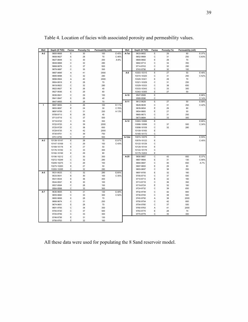
Table 4. Location of facies with associated porosity and permeability values.
All these data were used for populating the 8 Sand reservoir model.
Well Depth (ft TVD) Facies Porosity (%) Permeability (mD) Well Depth (ft TVD) Facies Porosity (%) Permeability (mD)A-2 9800-9808 E 30 100 E:45% A-7st 9633-9652 E 29 80 E:37%
9808-9827 E 28 70 C:46% 9652-9669 C 31 250 C:63%9827-9848 C 30 200 A:9% 9669-9682 E 28 709848-9868 C 32 280 9682-9714 C 34 3509868-9878 C 37 500 9714-9743 C 32 2809878-9887 C 35 350 9743-9756 E 30 1009887-9895 A 41 2000 A-8 10303-10315 E 27 50 E:48%9895-9898 C 32 280 10315-10320 C 31 250 C:52%9898-9904 A 40 2000 10320-10321 E 28 709904-9918 E 28 70 10321-10329 C 31 2509918-9922 C 32 280 10329-10333 C 38 6509922-9927 E 26 40 10333-10343 C 33 3009927-9936 E 29 80 10343-10355 E 27 509936-9941 C 29 150 A-10 9547-9589 E E:86%9941-9947 E 26 40 9589-9596 C C:14%9947-9955 E 28 70 A-11 9612-9628 E 27 50 E:58%
1 9687-9693 C 26 100 E:11% 9628-9639 C 31 250 C:42%9693-9697 E 24 30 C:76% 9639-9654 E 29 809697-9709 C 31 250 A:13% 9654-9665 E 27 509709-9713 E 26 40 9665-9673 C 31 2509713-9719 C 37 500 9673-9684 C 33 3009719-9722 C 35 350 A-12 10083-10086 E E:66%9722-9725 A 39 2000 10086-10098 C 37 500 C:34%9725-9729 C 38 650 10098-10109 C 32 2809729-9735 A 42 2000 10109-10165 E9735-9751 C 39 750 10165-10172 C9751-9759 C 37 500 A-12st 10074-10079 C E:55%
A-3 10139-10147 E 28 70 E:57% 10079-10122 E C:45%10147-10169 C 29 150 C:43% 10122-10129 C10169-10176 E 27 50 10129-10144 E10176-10182 C 33 300 10144-10179 C10182-10190 E 29 80 10179-10203 E10190-10212 C 35 350 A-25 9656-9667 C 43 800 E:37%10212-10249 C 32 280 9667-9684 E 31 130 C:56%10249-10275 C 29 150 9684-9687 C 40 650 A:7%10275-10283 E 27 50 9687-9693 E 29 8010283-10285 C 32 280 9693-9697 C 36 350
A-5 9531-9533 C 32 280 E:65% 9697-9705 E 32 1609533-9541 E 30 100 C:35% 9705-9710 C 37 5009541-9544 E 36 400 9710-9713 E 32 1609544-9557 E 30 100 9713-9719 C 36 3509557-9564 C 28 150 9719-9724 E 32 1609564-9568 C 33 300 9724-9732 C 39 650
A-7 9636-9655 E 31 130 E:48% 9732-9739 C 42 8009655-9660 C 33 300 C:52% 9739-9745 C 38 5009660-9668 E 28 70 9745-9750 A 38 20009668-9674 C 31 250 9750-9754 C 42 8009674-9691 E 28 70 9754-9760 C 37 5009691-9705 C 34 350 9760-9763 A 41 20009705-9720 C 37 500 9763-9770 E 28 709720-9746 C 33 300 9770-9779 C 35 3009746-9756 E 31 1309756-9763 E 32 160
40
CHAPTER IV
RESULTS
Location of the depositional environment
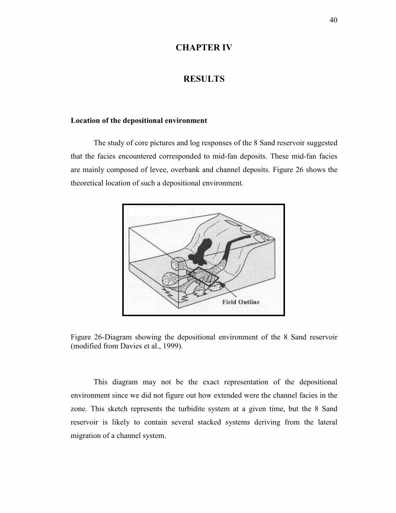
The study of core pictures and log responses of the 8 Sand reservoir suggested
that the facies encountered corresponded to mid-fan deposits. These mid-fan facies
are mainly composed of levee, overbank and channel deposits. Figure 26 shows the
theoretical location of such a depositional environment.
Figure 26-Diagram showing the depositional environment of the 8 Sand reservoir(modified from Davies et al., 1999).
This diagram may not be the exact representation of the depositional
environment since we did not figure out how extended were the channel facies in the
zone. This sketch represents the turbidite system at a given time, but the 8 Sand
reservoir is likely to contain several stacked systems deriving from the lateral
migration of a channel system.
41
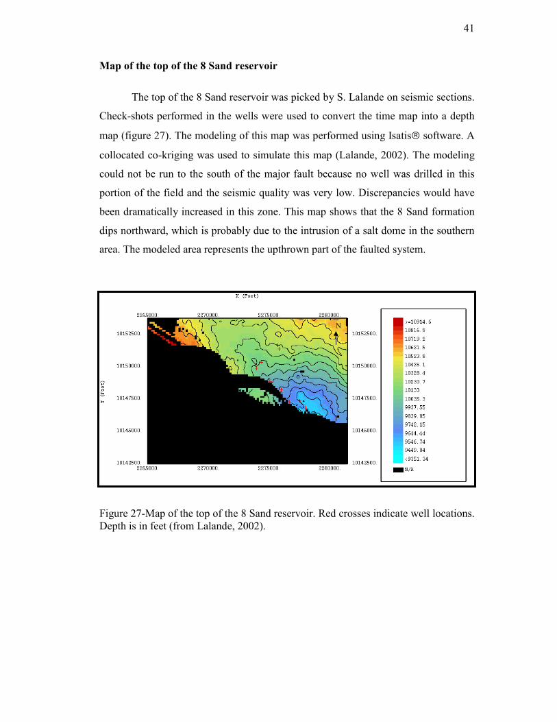
Map of the top of the 8 Sand reservoir
The top of the 8 Sand reservoir was picked by S. Lalande on seismic sections.
Check-shots performed in the wells were used to convert the time map into a depth
map (figure 27). The modeling of this map was performed using Isatis� software. A
collocated co-kriging was used to simulate this map (Lalande, 2002). The modeling
could not be run to the south of the major fault because no well was drilled in this
portion of the field and the seismic quality was very low. Discrepancies would have
been dramatically increased in this zone. This map shows that the 8 Sand formation
dips northward, which is probably due to the intrusion of a salt dome in the southern
area. The modeled area represents the upthrown part of the faulted system.
Figure 27-Map of the top of the 8 Sand reservoir. Red crosses indicate well locations.Depth is in feet (from Lalande, 2002).
N
42
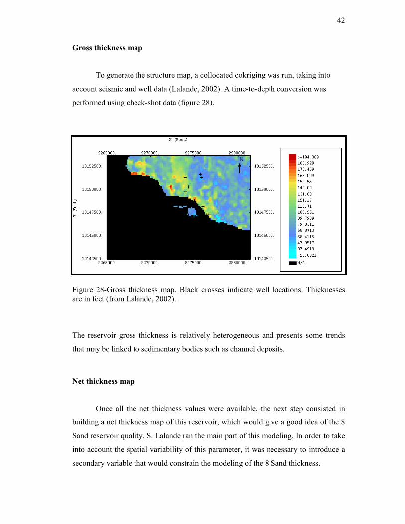
Gross thickness map
To generate the structure map, a collocated cokriging was run, taking into
account seismic and well data (Lalande, 2002). A time-to-depth conversion was
performed using check-shot data (figure 28).
Figure 28-Gross thickness map. Black crosses indicate well locations. Thicknessesare in feet (from Lalande, 2002).
The reservoir gross thickness is relatively heterogeneous and presents some trends
that may be linked to sedimentary bodies such as channel deposits.
Net thickness map
Once all the net thickness values were available, the next step consisted in
building a net thickness map of this reservoir, which would give a good idea of the 8
Sand reservoir quality. S. Lalande ran the main part of this modeling. In order to take
into account the spatial variability of this parameter, it was necessary to introduce a
secondary variable that would constrain the modeling of the 8 Sand thickness.
N
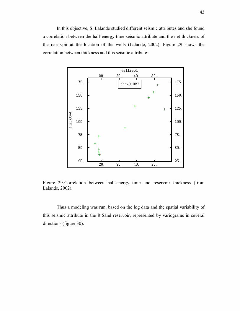
43
In this objective, S. Lalande studied different seismic attributes and she found
a correlation between the half-energy time seismic attribute and the net thickness of
the reservoir at the location of the wells (Lalande, 2002). Figure 29 shows the
correlation between thickness and this seismic attribute.
Figure 29-Correlation between half-energy time and reservoir thickness (fromLalande, 2002).
Thus a modeling was run, based on the log data and the spatial variability of
this seismic attribute in the 8 Sand reservoir, represented by variograms in several
directions (figure 30).
44
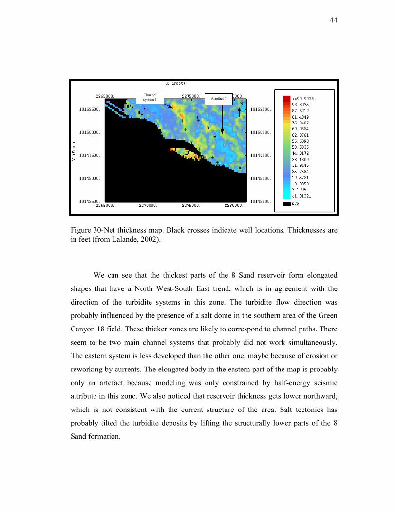
Figure 30-Net thickness map. Black crosses indicate well locations. Thicknesses arein feet (from Lalande, 2002).
We can see that the thickest parts of the 8 Sand reservoir form elongated
shapes that have a North West-South East trend, which is in agreement with the
direction of the turbidite systems in this zone. The turbidite flow direction was
probably influenced by the presence of a salt dome in the southern area of the Green
Canyon 18 field. These thicker zones are likely to correspond to channel paths. There
seem to be two main channel systems that probably did not work simultaneously.
The eastern system is less developed than the other one, maybe because of erosion or
reworking by currents. The elongated body in the eastern part of the map is probably
only an artefact because modeling was only constrained by half-energy seismic
attribute in this zone. We also noticed that reservoir thickness gets lower northward,
which is not consistent with the current structure of the area. Salt tectonics has
probably tilted the turbidite deposits by lifting the structurally lower parts of the 8
Sand formation.
N
Channelsystem 1 Artefact ?
45
Well correlations
Correlation between wells led us to obtain three cross sections. These cross-
sections only represent one of the possible interpretations that can be performed from
our dataset. A lot of uncertainties still remain about the channel location and the
relationship between the bodies A and B. Amplitude map shows that there is an
unconformity at the boundary between the two bodies, which may be related to a
facies change. In some seismic cross-sections, body A seems to overlap body A. But
this feature could not be checked in all the cross-sections. We tried to focus on the
continuity of the reflectors inside the reservoir but it was very difficult to draw
conclusions, due to the low quality of the seismic data (Lalande, 2002). We assumed
that channels presented shingled stacking, but we could not figure out how extended
were the channel deposits. The only information came from well A-2 in which we
observed a 8 feet thick channel deposit. This confirmed that channel stacking was not
vertical.
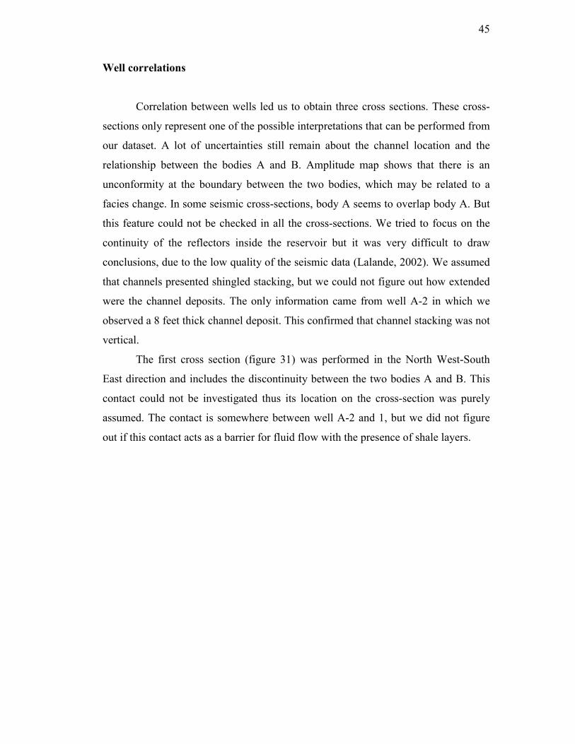
The first cross section (figure 31) was performed in the North West-South
East direction and includes the discontinuity between the two bodies A and B. This
contact could not be investigated thus its location on the cross-section was purely
assumed. The contact is somewhere between well A-2 and 1, but we did not figure
out if this contact acts as a barrier for fluid flow with the presence of shale layers.
46
Figu
re 3
1-C
ross
-sec
tion
1 fr
om w
ell c
orre
latio
n. It
s loc
atio
n is
indi
cate
d in
figu
re 2
9.
Faci
es A
(cha
nnel
)
Faci
es C
(lev
ee)
Faci
es E
(ove
rban
k)
Sout
h-E
ast
Nor
th-W
est
2260
ft16
50ft
1070
ft
Con
tact
bet
wee
nB
odie
s A a
nd B
?
100
ft
47
Figu
re 3
2-C
ross
-sec
tion
2 fr
om w
ell c
orre
latio
n. It
s loc
atio
n is
indi
cate
d in
figu
re 3
3.
9500
Faci
es A
(cha
nnel
)
Faci
es C
(lev
ee)
Faci
es E
(ove
rban
k)
Wes
tE
ast
800
ft75
0ft
800
ft30
0ft
100
ft
48
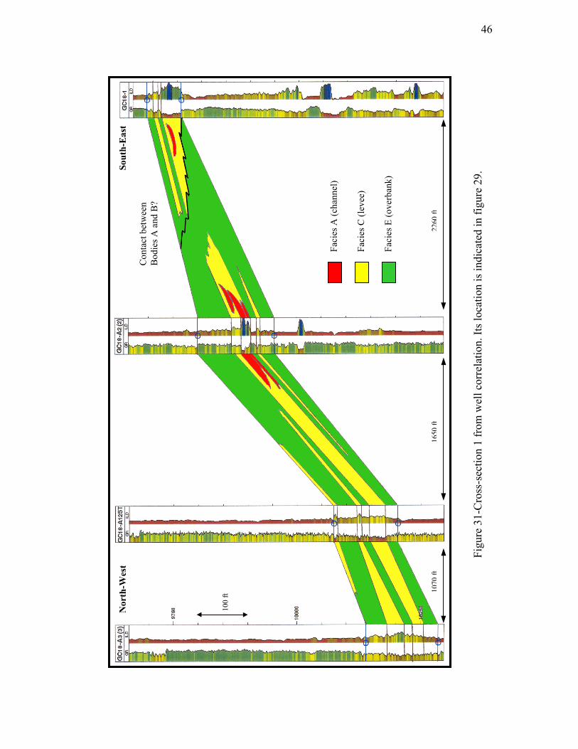
The second cross-section (figure 32) has a West-East trend and represents a lower-
quality part of the 8 Sand reservoir. It is obvious that reservoir quality gets poorer
eastward since the deposits are further from channel path. It confirmed that body A
does not contain facies as good as in body B, maybe because it was partially eroded
by overlying formations. There is no evidence of channel deposits. Well A-25 was
assumed to be close to channel edges. Figure 33 shows the location of these cross-
sections.
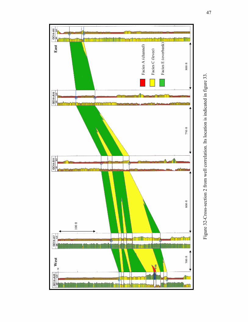
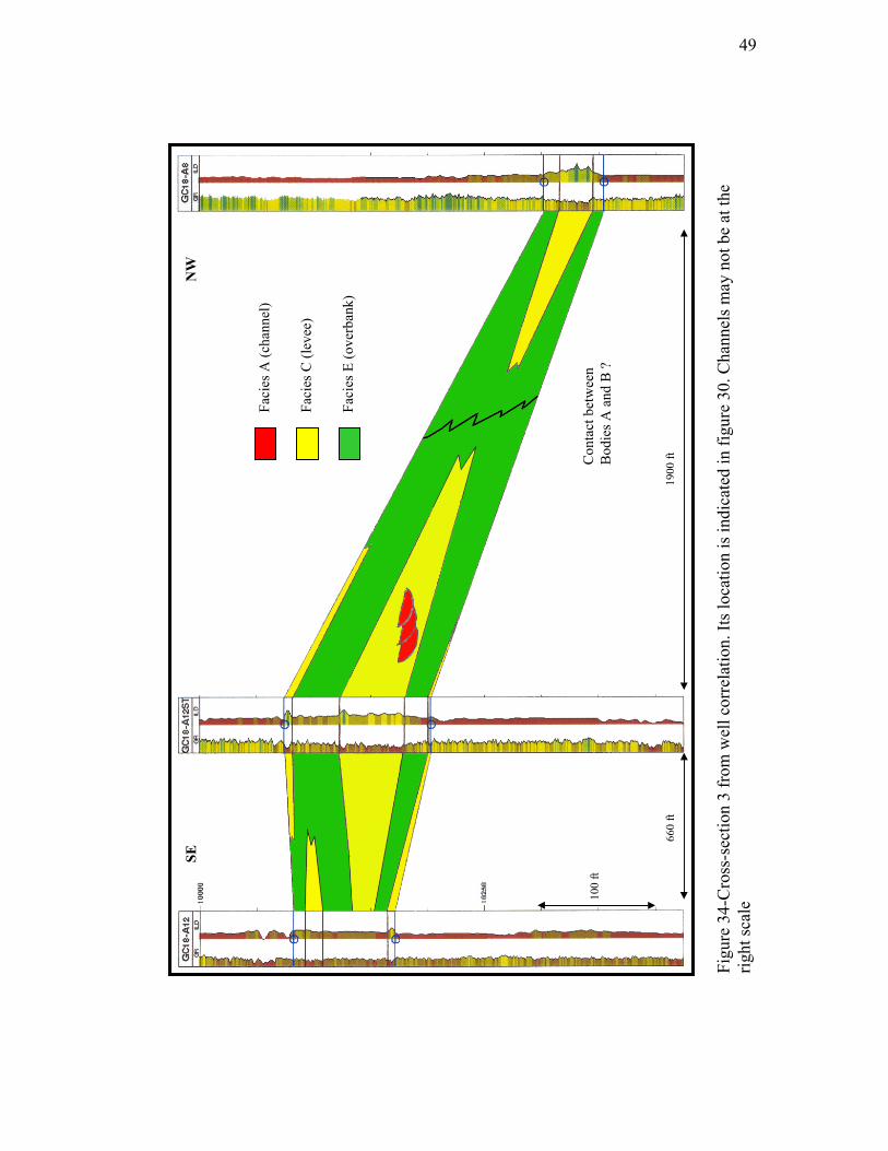
The third cross-section (figure 34) is perpendicular to the channel system
path. Wells A-12 and A-12st were drilled in body B while well A-8 crossed body A.
Log response is better in A-12st than in A-12 thus we inferred that channel deposits
were located to the East of A-12st. Contact between the two bodies could not be
investigated so a lot of uncertainties remain in this zone.
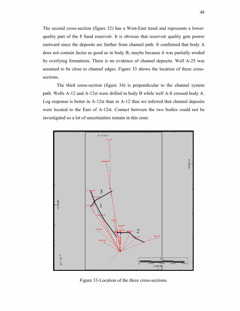
Figure 33-Location of the three cross-sections.
1
2
3
49
Figu
re 3
4-C
ross
-sec
tion
3 fr
om w
ell c
orre
latio
n. It
s loc
atio
n is
indi
cate
d in
figu
re 3
0. C
hann
els m
ay n
ot b
e at
the
right
scal
e
Faci
es A
(cha
nnel
)
Faci
es C
(lev
ee)
Faci
es E
(ove
rban
k)
SEN
W
1900
ft66
0ft
Con
tact
bet
wee
nB
odie
s A a
nd B
?10
0 ft
50
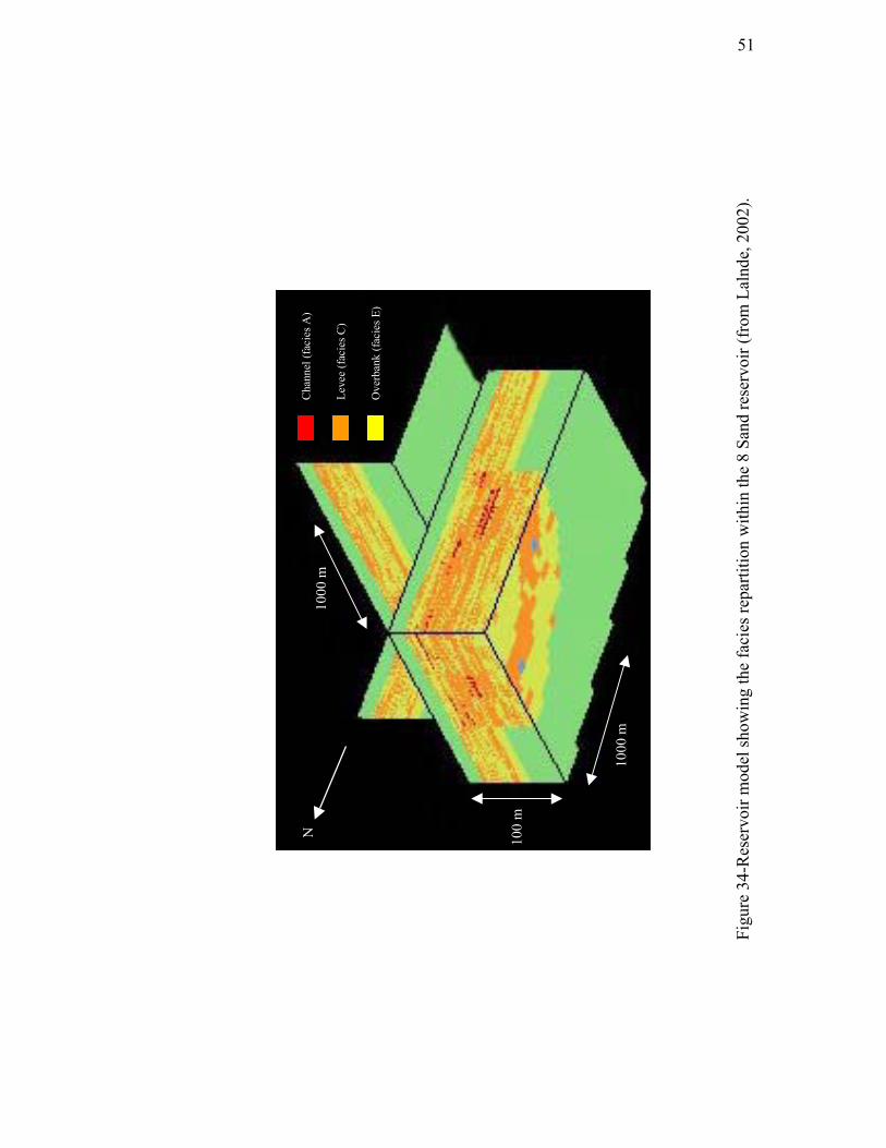
3-D reservoir model
The final step consisted in building a reservoir model with the facies, porosity
and permeability values. Seismic attributes could not be used because seismic
resolution is not high enough to account for variability inside a 100 ft-thick reservoir.
Thus a truncated gaussian simulation, based on facies percentages, was performed to
propagate the values available at the well locations. The area was divided into 3
distinct zones in which three independent simulations were performed (Lalande,
2002). The software used for this modeling did not allow taking into account with
precision the 8 Sand reservoir shape, but the model obtained gives a good idea of the
internal organization of the reservoir.
Figure 35 shows a view of this model, with facies A, C and E populating the
reservoir. We can see the shape of the channel system that constitutes the main part
of body B (western part). The channel path is curved in this zone, which is probably
induced by a topographic high due to salt tectonics. In this model there is no channel
deposit in the eastern part of the reservoir, but uncertainties are large in this area.
This 3-D model needs to be upscaled before running a reservoir simulation. Later on
porosity and permeability maps will be performed, based on the results in table 3.
51
Figu
re 3
4-R
eser
voir
mod
el sh
owin
g th
e fa
cies
repa
rtitio
n w
ithin
the
8 Sa
nd re
serv
oir (
from
Lal
nde,
200
2).
Cha
nnel
(fac
ies A
)
Leve
e (f
acie
s C)
Ove
rban
k (fa
cies
E)
100
m
N10
00 m
1000
m
52
CHAPTER V
DISCUSSION
Uncertainties about reservoir shape
The main uncertainties concern the spatial extension of the 8 Sand reservoir.
The low quality and the limited extent of seismic sections did not allow S. Lalande
determining the limits of the reservoir. Most of the wells are concentrated in the same
part of the field, which prevented from characterizing with precision the outer parts
of the reservoir. The thickness map may be an indicator of the areal extent of this
reservoir. It is reasonable to think that both structural and stratigraphic closure
determine the extension of the 8 Sand reservoir. The stratigraphic closure should be
done by hemipelagic shale that from the “background” of the sedimentation in the
basin. Salt diapirs are also likely to border the reservoir, especially in the southern
part of the area. Communication with upper and lower reservoirs could not be
demonstrated. Well test data showed that the North West-south East main fault
should be a sealing boundary. The lack of data in the southern part of the reservoir
and the bad quality of seismic data prevented us from investigating this part of the
reservoir.
Continuity inside the reservoir
Previous studies pointed out the existence of two main bodies in the 8 Sand
reservoir: they are called 8a and 8b. A-2, A-3 and A-12 are the wells that cross the 8b
part of the 8 Sand reservoir, which indicates that this body is located in the northern-
west part of the Green Canyon field. Figure 27 shows a discontinuity between the
two major sand accumulations, which is likely to be the boundary between the two
bodies. Seismic sections tend to show that body A overlies body B, but the poor
quality of the seismic signal in this area did not permit to be affirmative on this point.
Some pressure and production data were available for the part b of the 8 Sand, but we
53
did not figure out whether the two sand bodies were well connected or not. The
origin of these two bodies remains unclear. They may correspond to two channel
systems that were active simultaneously. But the second channel system might have
been active after the first one, eroding or not a part of the channel fill that had been
deposited previously. Interaction between the different channel systems is a key-
point because it defines how the two bodies are connected between each other. Some
previous studies concluded that they should be some communication between the two
bodies. We also noticed that body A might have been partially eroded after its
deposition, which could explain the bad seismic response. There is no evidence of
channel deposits in this area. Boundaries between levee and overbank deposits are
not likely to represent barriers for fluid flow because the change of facies is usually
progressive. Channel width is also misunderstood, but the channels are probably
several hundred feet wide. The associated levees and overbank should be more than
one thousand feet wide, but this is only an order of magnitude.
Recommendations for future 8 Sand reservoir simulation
The 8 Sand reservoir study led to several conclusions about the way of
running a future reservoir simulation.
First the channel locations should be taken into account during history
matching. The log and seismic data did not allow us figuring out how extended was
this facies.
Log data confirmed that there is a large aquifer at about 10350 feet. It
confirmed that this active aquifer is likely to represent a good pressure support during
reservoir production.
The kv/kh ratio should be low enough to take into account the laminated
nature of sediments in the 8 Sand reservoir. This value should be less than 0,05.
This reservoir is not fractured, which could prevent early water and gas
breakthrough during production. The main southern fault is assumed to be a sealing
fault, according to well test results.
54
CHAPTER VI
CONCLUSIONS
Analysis of core and well log data in the Green Canyon 18 field, Gulf of
Mexico, allowed characterizing the Upper Pliocene 8 Sand reservoir. It was
deposited in one of the mini-basins that were created by salt tectonics. This reservoir
is made of fine-grained turbidite deposits that are mainly composed of alternating
sand/silt and shale layers. The major part of the facies could be associated with levee
and overbank deposits, with some channel deposits deriving from narrow,
meandering and laterally migrating turbidite channels fed by shelf material. Then this
formation was probably tilted and deformed by fault and salt tectonics, as it is
suggested by the presence of a major extensive fault in the southern part of the field
and the discrepancies between current structure and reservoir thickness.
The high porosity and horizontal permeability values measured in core data,
at least in facies A and C, are mainly due to the absence of diagenetic features in
these unconsolidated sediments, and thus mainly depend on the depositional
conditions of the turbidite currents. Two channel systems were probably active at
different times, and one of them was assumed to having been eroded by new turbidity
currents later on. The best facies are located in body B, with a presumed shingled
stacking of channels. Cross-sections built from well correlation show that facies are
likely to be laterally continuous, even if interactions between the two bodies could
not be investigated. All this information will result in the building of a 3-D model of
the 8 Sand reservoir.
Large uncertainties still remain in the reservoir geological description, due to
the lack of data describing the 8 Sand reservoir. Nevertheless several
recommendations could be raised for a future reservoir simulation. One of the most
important is the low kv/kh ratio resulting from the laminated structure of sediments.
No thick shale layer could be highlighted in the reservoir, but some hemipelagic
shales might be present in the reservoir.

55
REFERENCES CITED
Beard, D. C., and P. K. Weyl, 1973, Influence of texture on porosity andpermeability of unconsolidated sand: AAPG Bulletin, v. 57, p. 349-369.
Bouma, A. H., W. R. Normark, and N. E. Barnes, eds., 1985a, Submarine fans andrelated turbidite systems: New-York, Springer-Verlag, 351 p.
Bouma, A. H., et al., 1985b, Mississipi Fan : Leg 96 program and principal results, inA. H. Bouma, W. R. Normark, and N. E. Barnes, eds., 1985a, Submarine fans andrelated turbidite systems: New-York, Springer-Verlag, p. 247-252.
Bouma, A. H., C. E. Stelting, and J. M. Coleman, 1985c, Mississipi Fan, Gulf ofMexico, in A. H. Bouma, W. R. Normark, and N. E. Barnes, eds., 1985a, Submarinefans and related turbidite systems: New-York, Springer-Verlag, p. 143-150.
Bouma, A. H., and H. deV. Wickens, 1994, Tanqua Karoo, ancient analog for fine-grained submarine fans, in P. Weimer, A. H. Bouma, and B. F. Perkins, eds.,Submarine fans and turbidite systems: sequence stratigraphy, reservoir architectureand production characteristics; Gulf of Mexico and international: Gulf Coast SectionSEPM 15th Annual Research Conference Proceedings, p. 23-34.
Bouma, A. H., G. H. Lee, O. van Antwerpen, and T. C. Cook, 1995a, Channelcomplex architecture of fine-grained submarine fans at the base-of-slope: Gulf CoastAssociation of Geological Societies Transactions, v. 65, p. 65-70.
Bouma, A. H., H. D. Wickens, and J. M. Coleman, 1995b, Architecturalcharacteristics of fine-grained submarine fans: a model applicable to the Gulf ofMexico: Gulf Coast Association of Geological Societies Transactions, v. 65, p. 71-75.
Bouma A. H., 2000, Fine-grained, mud-rich turbidite systems: model and comparisonwith coarse-grained, sand-rich systems, in A. H. Bouma and C. G. Stone, eds., Fine-grained turbidite systems, AAPG Memoir 72/SEPM Special Publication 68, p. 9-20.
Brenchley, P. J., and G. Newall, 1977, The significance of contorted bedding in theUpper Ordovician sediments of the Oslo region, Norway: Journal of SedimentaryPetrology, v. 47, p. 819-833.
Brinkmann, P. E., G. J. Barbler, and W. Rodriguez, 1985, Design and installation ofa 20-slot template in the Gulf of Mexico in 760 ft of water: paper SPE 14579,presented at the 1985 OTC, Houston, 6-9 May, p. 99-103.
Damuth, J. E., R. D. Flood, R. O. Kowsmann, R. H. Belderson, and M. A. Goriniet,1988, Anatomy and growth pattern of Amazon deep-sea fan as revealed by long-
56
range side-scan sonar (GLORIA) and high-resolution seismic studies: AAPGBulletin, v. 72, p. 885-911.
Darling, H. L., and R. M. Sneider, 1992, Production of low resistivity, low-contrastreservoirs, offshore Gulf of Mexico basin: Gulf Coast Association of GeologicalSocieties Transactions, v. 42, p. 73-88.
Davies, D. K., P. S. Hara, and J. J. Mondragon, 1999, Geometry, internalheterogeneity and permeability distribution in turbidite reservoirs, PlioceneCalifornia: paper SPE 56819, presented at the 1999 SPE Annual TechnicalConference and Exhibition, Houston, 3-6 October.
Dunham, L., 1993, Personal communication.
Lalande, S., 2002, Characterization of a thin-bedded reservoir in the Gulf of Mexico:an integrated approach: Master’s thesis, Texas A&M University, College Station,Texas, 60 p.
McPherson, J. G., 1982, Personal communication.
Menard, H. W., 1955, Deep-sea channels, topography, and sedimentation: AAPGBulletin, v. 39, p. 236-255.
Mutti, E., and W. R. Normark, 1987, Comparing examples of modern and ancientturbidite systems: problems and concepts, in J. K. Leggett and G. G. Zuffa, eds.,Marine clastic geometry: concepts and case studies: London, Graham and Troutman,p. 1-38.
Mutti, E., and W. R. Normark, 1991, An integrated approach to the study of turbiditesystems, in P. Weimer, and M. H. Link, eds., Seismic facies and sedimentaryprocesses of submarine fans and turbidite systems: New-York, Springer-Verlag, p.75-106.
Ostermeier, R. M., 1993, Deepwater Gulf of Mexico turbidites: compaction effectson porosity and permeability: paper SPE 26468, presented at the 1993 AnnualTechnical Conference and Exhibition, Houston, 3-6 October, p. 539-551.
Posamentier, H. W., M. T. Jervey, and P. R. Vail, 1988, Eustatic controls on clasticdeposition 1-conceptual framework, in C. K. Wilgus, B. S. Hasting, C. G. S.C.Kendall, H. W. Posamentier, C. A. Ross, and J. C. Van Wagoner, eds., Sea levelchanges: an integrated approach: SEPM Special Publication 42, p. 109-124.
Reading, H. G., and M. Richards, 1994, Turbidite systems in deep-water basinmargins classified by grain size and feeder system: AAPG Bulletin, v. 78, p. 792-822.
57
Reedy, G. K., and C. F. Pepper, 1996, Analysis of finely laminated deep marineturbidites: integration of core and log data yields a novel interpretation model: paperSPE 36506, presented at the 1996 Annual Technical Conference and Exhibition,Denver, Colorado, 6-9 October, p. 119-127.
Reineck, H. E., and I. B. Singh, 1973, Depositional sedimentary environments: New-York, Springer-Verlag, 439 p.
Stelting, C. E., A. H. Bouma, and C. G. Stone, 2000, Fine-grained turbidite systems:overview, in A. H. Bouma and C. G. Stone, eds., fine-grained turbidite systems,AAPG Memoir 72/SEPM Special Publication 68, p. 1-8.
Weimer, P., P. Varnai, F. M. Budhijanto, Z. M. Acosta, and R. E. Martinez, 1998,Sequence stratigraphy of Pliocene and Pleistocene turbidite systems, Northern GreenCanyon and Ewing Bank (offshore Louisiana), Northern Gulf of Mexico: AAPGBulletin, v. 82, p. 918-960.
Williams, L. I., 2000, Personal communication.
58
VITA
Matthieu Plantevin
Date of birth: March 13, 1976
Education: M.S. Geology, Texas A&M University, 2002M.S. Reservoir Geoscience and Engineering, IFP School,France, 2002B.Sc. (engineering degree) Geology, Ecole NationaleSuperieure de Geologie, France, 2000
Experience: January to May 2002-Graduate Assistant Research, PetroleumEngineering Department, Texas A&M University.
January to August 2000- Training period within TOTAL FINA(Paris) with reservoir characterization objective by studyingWest Africa trend curves.
Summer 1999- Training period within ELF EP (Pau, France)based on the underlining of Low Resistivity Sand typereservoirs (wireline logging studies).
Mailing address: 31, rempart Saint Pierre71100 Chalon sur SaoneFrance