Embed Size (px)
Citation preview
Naval Oceanographic OfficeStennis Space Technical ReportCenter TR 306MS 39522-5001 June 1992 AD-A255 207
ll tlltlllillllll llllll!TR 306
CHARACTERIZATION OF THE BOTTOM SEDIMENTVELOCITY-DEPTH RELATIONSHIP FOR THESOMALI BASIN AND THE ARABIAN SEA
NELSON J. LETOURNEAUACOUSTICS DIVISION
DTICS ELECTE
SEP 15 1992 DSAE
Approved for public release; 9t2"25 ý146distribution Is unlimited.
Prepared under the authority of92 Commander,
4 4 Naval Oceanography Command
* I
FOREWORD IKnowledge of the geoacoustic parameters of the sea floor is
required for accurate prediction of sound propagation in bottom-limited areas. This technical report discusses the acquisitionof wide angle bottom reflection data and the development ofbottom sediment velocity versus depth curves and functions fromthese data in the Somali Basin and the Arabian Sea.
Captain, .S NavyCommanding Officer I
]IIIII]IIIIII
REPORT DOCUMENTATION PAGE CN'r
1. AGENCt USE ON.Y Lea, ' b .-.. 2 REPORT DATE 3 REPORT TYPE AND DATES CO EREDI June 1992
ICharacterization of the Bottom Sediment Velocity-DepthRelationship for the Somali Basin and the Arabian Sea
Nelson J. LeTourneau
7.iPERC-M% 0PrzI.! > ' E:.N AN: ADD ý$ 15) CP :'O4N'2AT!ON
* Naval Oceanographic OfficeStennis Space Center, MS 39522-5001 TR 306
Commander, Naval Oceanography CommandStennis Space Center, MS 39529-5000
I _ _ _ -..- -.- _ _ _ __. _ _ _ _ _
Approved for public release;distribution is unlimited.
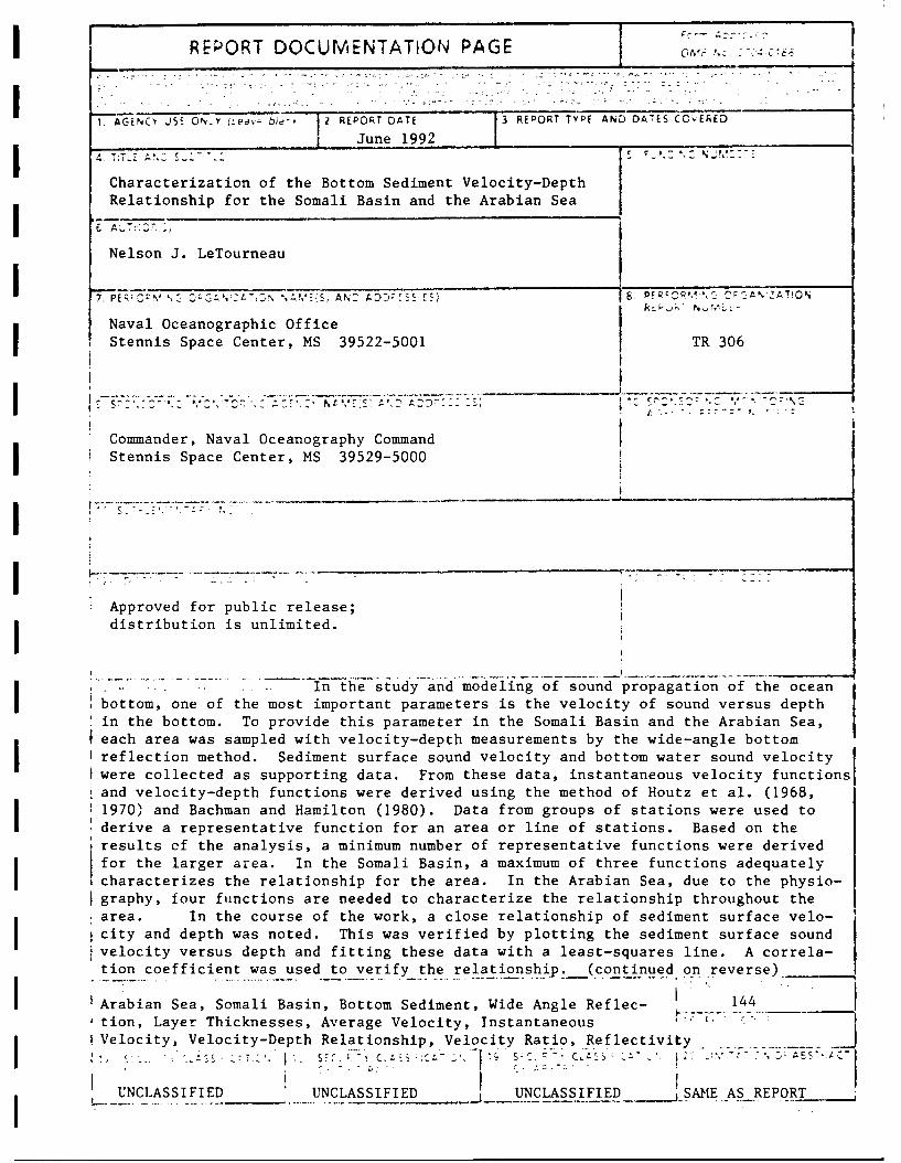
.... -.. . .... In the study and modeling of sound propagation of the oceanI bottom, one of the most important parameters is the velocity of sound versus depthin the bottom. To provide this parameter in the Somali Basin and the Arabian Sea,
i each area was sampled with velocity-depth measurements by the wide-angle bottomI reflection method. Sediment surface sound velocity and bottom water sound velocity
i were collected as supporting data. From these data, instantaneous velocity functionsand velocity-depth functions were derived using the method of Houtz et al. (1968,1970) and Bachman and Hamilton (1980). Data from groups of stations were used toderive a representative function for an area or line of stations. Based on theresults ef the analysis, a minimum number of representative functions were derivedfor the larger area. In the Somali Basin, a maximum of three functions adequatelycharacterizes the relationship for the area. In the Arabian Sea, due to the physio-
I graphy, four functions are needed to characterize the relationship throughout thearea. In the course of the work, a close relationship of sediment surface velo-I city and depth was noted. This was verified by plotting the sediment surface sound
ivelocity versus depth and fitting these data with a least-squares line. A correla-tion coefficient was used to verify the relationshi9 . (continued on reverse)__
Arabian Sea, Somali Basin, Bottom Sediment, Wide Angle Reflec- -144
Ition, Layer Thicknesses, Average Velocity, Instantaneous C" -"
!Velocity, Velocity-Depth Relationship, Velocity Ratio, Reflectivity..................
UN S IU CLASSIFIED I CLASSIFIED _ AR AESPOR CT
UNCLASSIFIED -UNCLASSIFIED JUNCLASSIFIED _ SAMEASREPORT~
ITR 306 I
REPORT DOCUMENTATION PAGE (CON.) I
Block 13 (Continued):
This relationship is believed to be due to the water included in the samplescored, thus the bottom water velocity versus depth was plotted and fittedwith a least-squares line. The slope of the lines for the sediment velocityversus depth and the bottom water velocity versus depth are compared. Inboth the Somali Basin and the Arabian Sea, the two quantities are nearlyidentical. Thus, it is concluded that the sediment surface sound velocityis definitely a function of depth in deep water areas.
IIIII
IIIII
ii
CHARACTERIZATION OF THE BOTTOM SEDIMENT
VELOCITY-DEPTH RELATIONSHIP FOR
THE SOMALI BASIN AND THE ARABIAN SEA
A DISSERTATION SUBMITTED TO THE GRADUATE DIVISION OF THEUNIVERSITY OF HAWAII IN PARTIAL FULFILLMENT
OF THE REQUIREMENTS FOR THE DEGREE OF
DOCTOR OF PHILOSOPHY
IN
GEOLOGY AND GEOPHYSICS
MAY 1991
By
Nelson J. LeTourneau
Dissertation Committee
Frederick Duennebier, ChairmanPow F. Fan
Murli H. ManghnaniGregory Mooze
Alexander Malahoff
iii
IIII
We certify that we have read this dissertation and that,
in our opinion, it is satisfactory in scope and quality as
a dissertation for the degree of Doctor of Philosophy in i
Geology and Geophysics.
III
DISSERTATION COMMITTEE
Chairperson I
____I
I
I
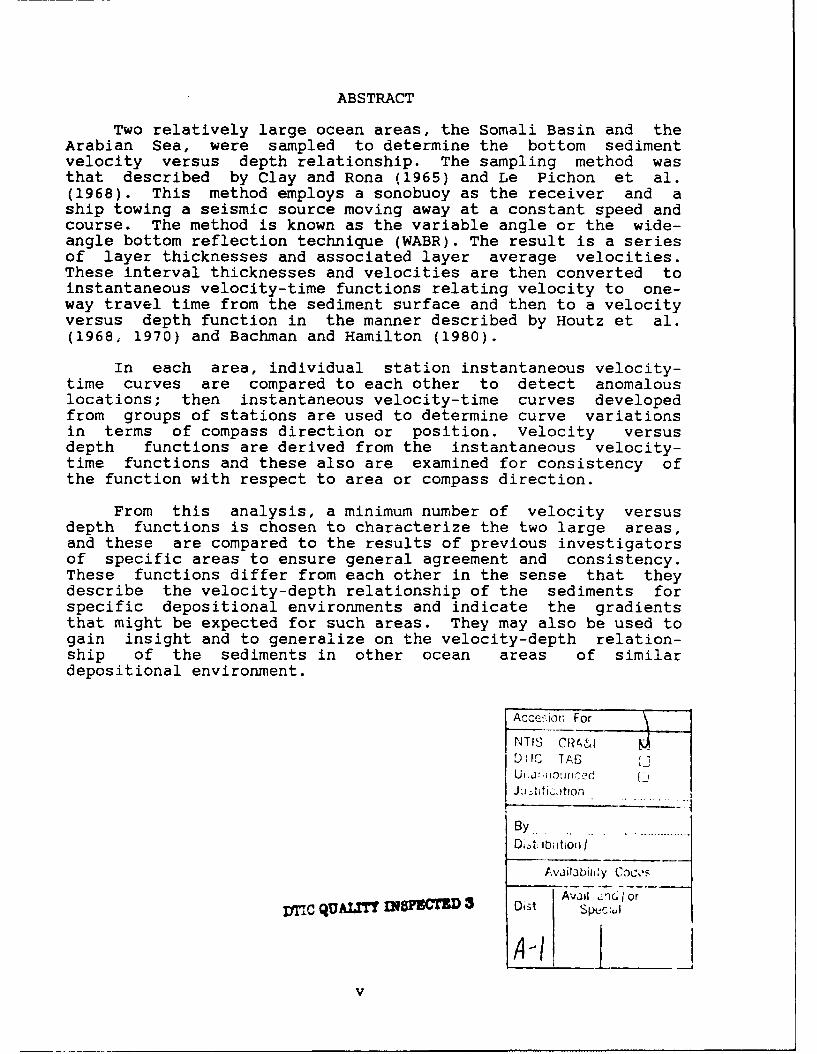
ABSTRACT
Two relatively large ocean areas, the Somali Basin and theArabian Sea, were sampled to determine the bottom sedimentvelocity versus depth relationship. The sampling method wasthat described by Clay and Rona (1965) and Le Pichon et al.(1968). This method employs a sonobuoy as the receiver and aship towing a seismic source moving away at a constant speed andcourse. The method is known as the variable angle or the wide-angle bottom reflection technique (WABR). The result is a seriesof layer thicknesses and associated layer average velocities.These interval thicknesses and velocities are then converted toinstantaneous velocity-time functions relating velocity to one-way travel time from the sediment surface and then to a velocityversus depth function in the manner described by Houtz et al.(1968; 1970) and Bachman and Hamilton (1980).
In each area, individual station instantaneous velocity-time curves are compared to each other to detect anomalouslocations; then instantaneous velocity-time curves developedfrom groups of stations are used to determine curve variationsin terms of compass direction or position. Velocity versusdepth functions are derived from the instantaneous velocity-time functions and these also are examined for consistency ofthe function with respect to area or compass direction.
From this analysis, a minimum number of velocity versusdepth functions is chosen to characterize the two large areas,and these are compared to the results of previous investigatorsof specific areas to ensure general agreement and consistency.These functions differ from each other in the sense that theydescribe the velocity-depth relationship of the sediments forspecific depositional environments and indicate the gradientsthat might be expected for such areas. They may also be used togain insight and to generalize on the velocity-depth relation-ship of the sediments in other ocean areas of similardepositional environment.
Accpaiorn For
NTIS CR4&IDuill TAG
ByD,*t: ibijtion I
AvaitabiWdy Coco's
3Avail an6 j or
DTIC QUALMI Sp.ciI
Aiuv
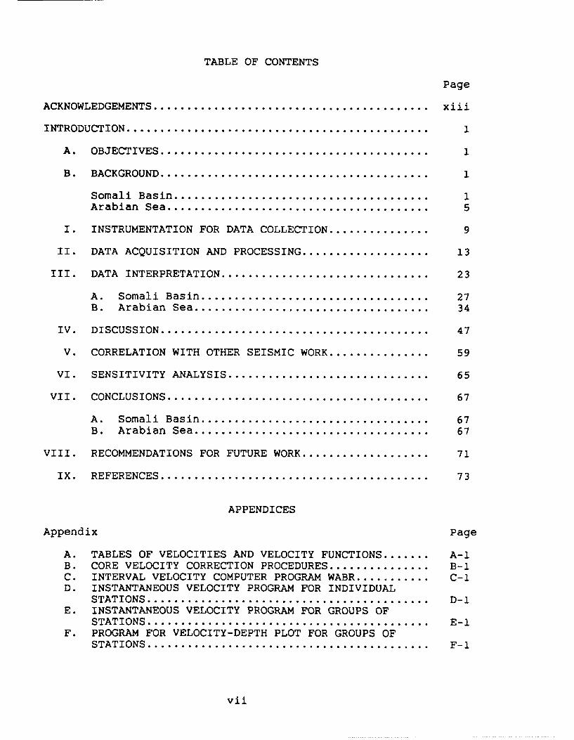
TABLE OF CONTENTS
Page
ACKNOWLEDGEMENTS ......................................... xiii
INTRODUCTION ............................................. 1
A. OBJECTIVES ........................................ 1
B. BACKGROUND ........................................ 1
Somali Basin ...................................... 1Arabian Sea ....................................... 5
I. INSTRUMENTATION FOR DATA COLLECTION .................. 9
II. DATA ACQUISITION AND PROCESSING ....................... 13
III. DATA INTERPRETATION ............................... 23
A. Somali Basin .................................. 27B. Arabian Sea ................................... 34
IV. DISCUSSION ........................................ 47
V. CORRELATION WITH OTHER SEISMIC WORK ................... 59
VI. SENSITIVITY ANALYSIS .............................. 65
VII. CONCLUSIONS ....................................... 67
A. Somali Basin .................................. 67B. Arabian Sea ................................... 67
VIII. RECOMMENDATIONS FOR FUTURE WORK ........................ 71
IX. REFERENCES ........................................ 73
APPENDICES
Appendix Page
A. TABLES OF VELOCITIES AND VELOCITY FUNCTIONS ....... A-iB. CORE VELOCITY CORRECTION PROCEDURES .................. B-iC. INTERVAL VELOCITY COMPUTER PROGRAM WABR ............. C-iD. INSTANTANEOUS VELOCITY PROGRAM FOR INDIVIDUAL
STATIONS .......................................... D-IE. INSTANTANEOUS VELOCITY PROGRAM FOR GROUPS OF
STATIONS .......................................... E-IF. PROGRAM FOR VELOCITY-DEPTH PLOT FOR GROUPS OF
STATIONS .......................................... F-i
vii
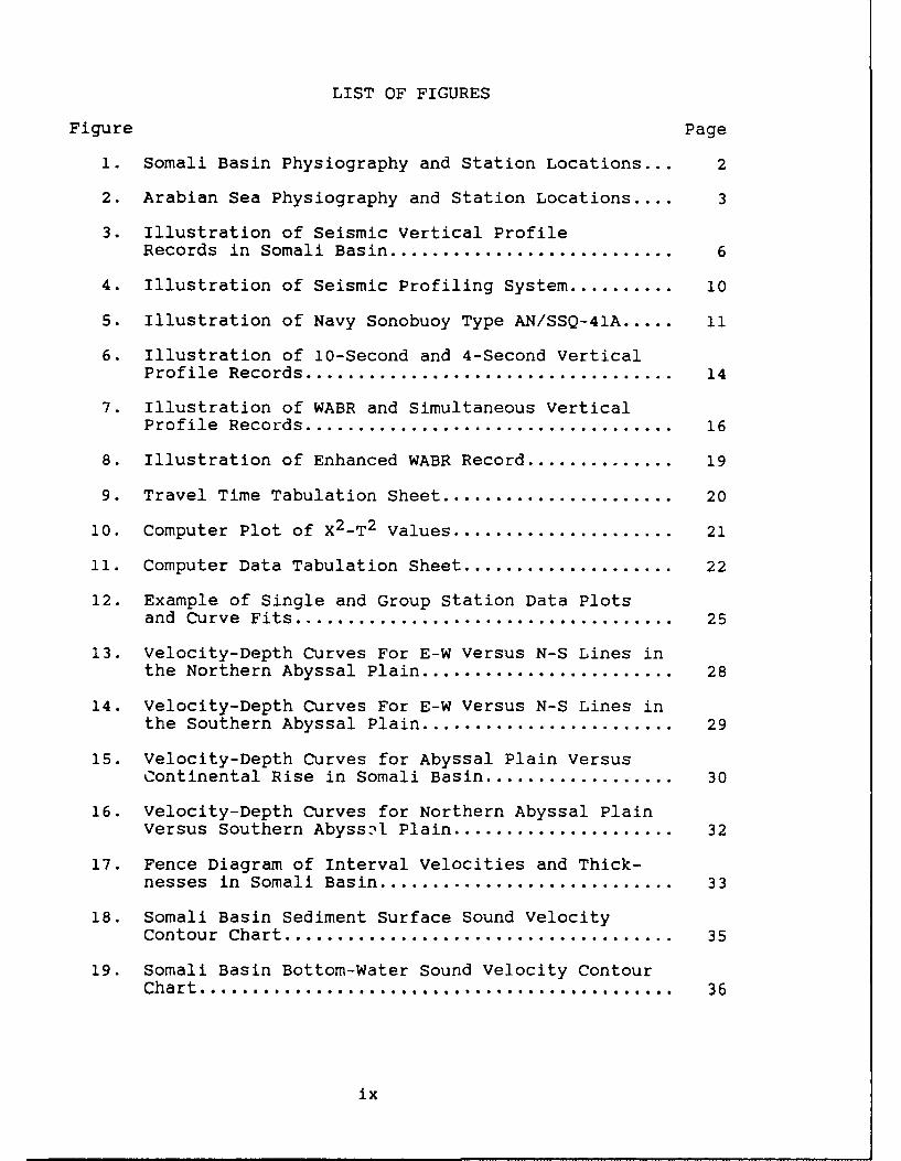
LIST OF FIGURES
Figure Page
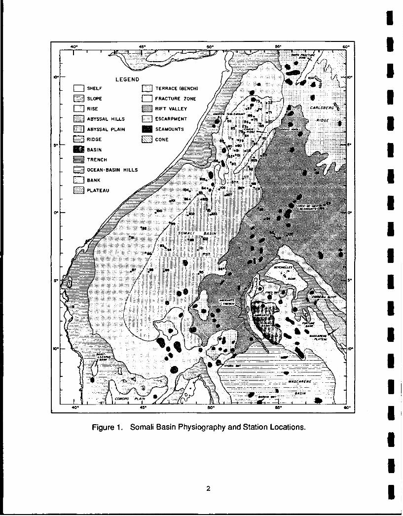
1. Somali Basin Physiography and Station Locations... 2
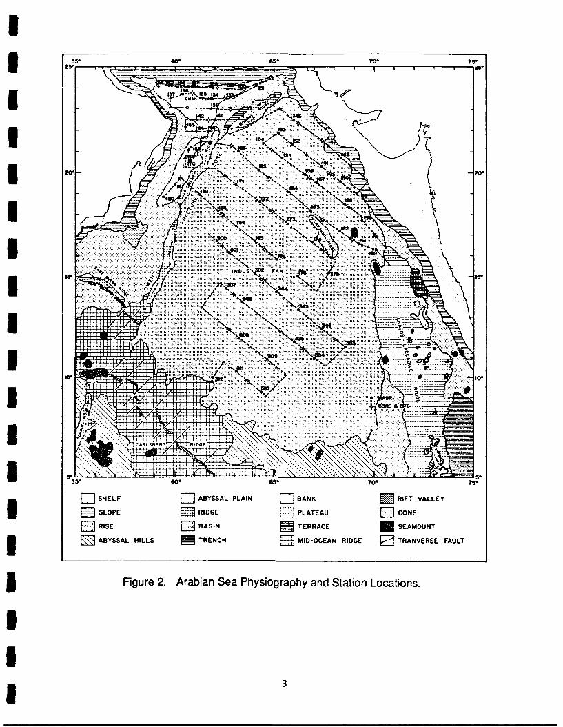
2. Arabian Sea Physiography and Station Locations .... 3
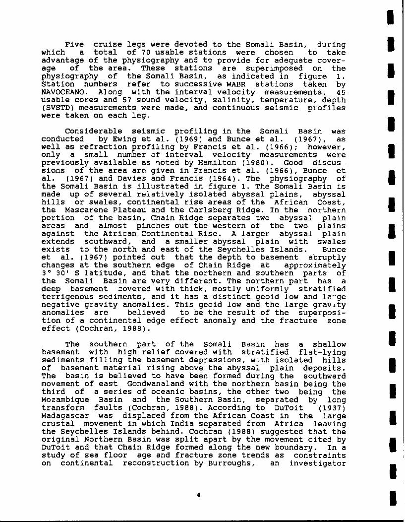
3. Illustration of Seismic Vertical ProfileRecords in Somali Basin ............................. 6
4. Illustration of Seismic Profiling System .......... 10
5. Illustration of Navy Sonobuoy Type AN/SSQ-41A ..... 11
6. Illustration of 10-Second and 4-Second VerticalProfile Records ...................................... 14
7. Illustration of WABR and Simultaneous VerticalProfile Records ...................................... 16
8. Illustration of Enhanced WABR Record .............. 19
9. Travel Time Tabulation Sheet ........................ 20
10. Computer Plot of X2 -T 2 Values ....................... 21
11. Computer Data Tabulation Sheet ...................... 22
12. Example of Single and Group Station Data Plotsand Curve Fits ....................................... 25
13. Velocity-Depth Curves For E-W Versus N-S Lines inthe Northern Abyssal Plain .......................... 28
14. Velocity-Depth Curves For E-W Versus N-S Lines inthe Southern Abyssal Plain .......................... 29
15. Velocity-Depth Curves for Abyssal Plain VersusContinental Rise in Somali Basin .................. 30
16. Velocity-Depth Curves for Northern Abyssal PlainVersus Southern AbyssMl Plain ....................... 32
17. Fence Diagram of Interval Velocities and Thick-nesses in Somali Basin .............................. 33
18. Somali Basin Sediment Surface Sound VelocityContour Chart ........................................ 35
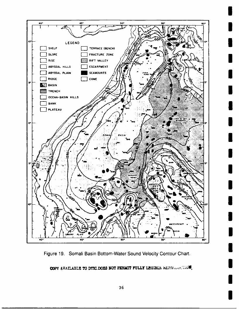
19. Somali Basin Bottom-Water Sound Velocity ContourChart ............................................. 36
ix
I
LIST OF FIGURES (CON.) 3Figure Page
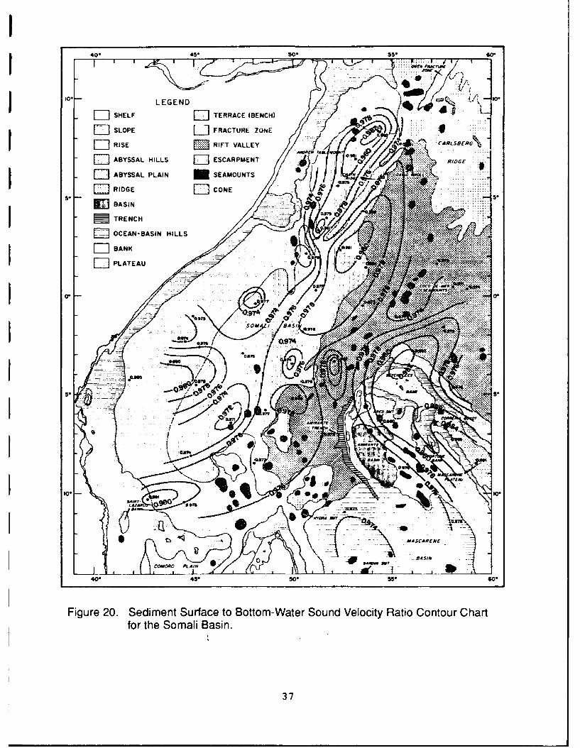
20. Sediment Surface to Bottom-Water Sound Velocity IRatio Contour Chart for the Somali Basin .......... 37
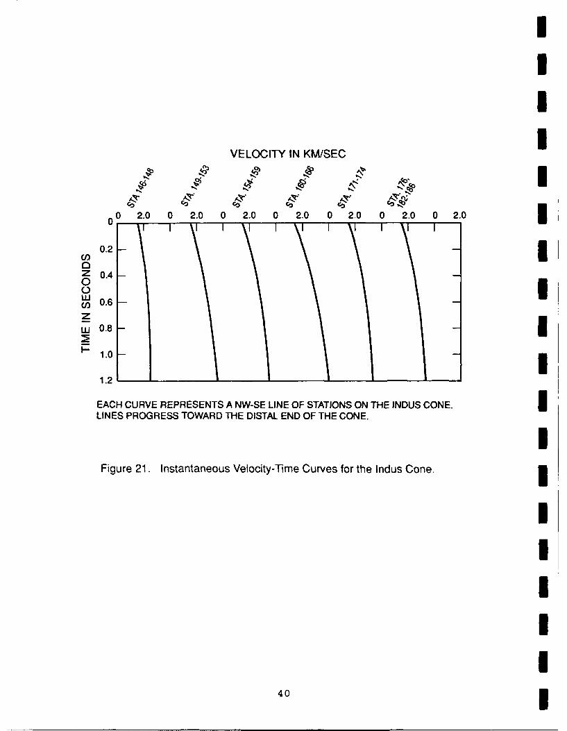
21. Instantaneous Velocity-Time Curves for the Indus iCone .................................................. 40
22. Fence Diagram of Interval Velocities and Thicknessesof the Arabian Sea ................................... 42
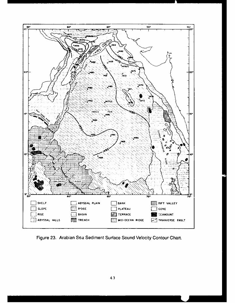
23. Arabian Sea Sediment Surface Sound VelocityContour Chart ........................................ 43
24. Arabian Sea Bottom-Water Sound VelocityContour Chart ........................................ 44
25. Sediment Surface to Bottom-Water Sound VelocityRatio Contour Chart of the Arabian Sea ............ 45 1
26. Sediment Surface velocity Versus Water Depthin the Somali Basin .................................. 48
27. Sediment Surface Velocity Versus Water Depthin the Arabian Sea ................................... 49
28. Instantaneous Velocity-Time Curves for NormalizedVersus Standard Data in the Somali Basin .......... 51
29. Instantaneous Velocity-Time Curves for Normalized iVersus Standard Data in the Arabian Sea ........... 52
30. Illustration of Hamilton's Table IIB .............. 54 331. Velocity Ratio Contour Chart Using
Hamilton's Tables .................................... 55
32. Plot of Reflection Coefficients Versus GrazingAngle ................................................. 57
33. Instantaneous Velocity-Time Functions for theSomali Basin ......................................... 60
34. Velocity-Depth Functions for the Indus Cone ....... 62
35. Instantaneous Velocity-Time Functions for the Indus 5Cone .................................................. 64
36. Illustration of Areas of Application for VariousVelocity-Depth Functions in Arabian Sea ........... 68 I
xI
LIST OF TABLES
Table Page
1. Velocity-Depth Functions .......................... A-3
A. Somali Basin ................................... A-3B. Arabian Sea .................................... A-3
2. Instantaneous Velocity Functions .................. A-4
A. Somali Basin ................................... A-4B. Arabian Sea .................................... A-4
3. Tabulation of Interval Velocities and LayerThicknesses in the Somali Basin ................... A-5
4. Tabulation of Interval Velocities and LayerThicknesses in the Arabian Sea .................... A-14
xi
ACKNOWLEDGEMENTS
The author gratefully acknowledges the encouragement andsupport of the Naval Oceanographic Office in this work and thehelp of many of the personnel of this organization who assistedin the acquisition and processing of the data. I thank themembers of my dissertation committee for their time, patienceand helpful suggestions. A special thanks to Dr. W.M. Adams,who opened doors long closed and got me on track again.
xiii
INTRODUCTION
A. OBJECTIVES
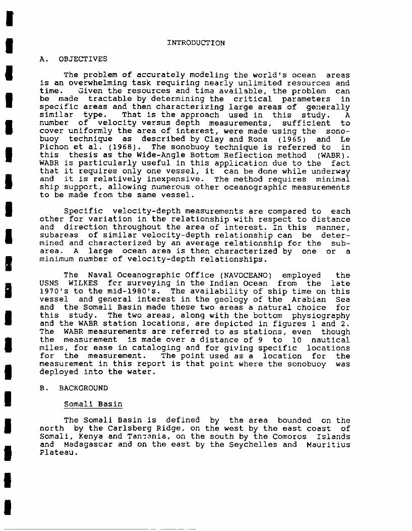
The problem of accurately modeling the world's ocean areasis an overwhelming task requiring nearly unlimited resources andtime. Given the resources and time available, the problem canbe made tractable by determining the critical parameters inspecific areas and then characterizing large areas of generallysimilar type. That is the approach used in this study. Anumber of velocity versus depth measurements, sufficient tocover uniformly the area of interest, were made using the sono-buoy technique as described by Clay and Rona (1965) and LePichon et al. (1968). The sonobuoy technique is referred to inthis thesis as the Wide-Angle Bottom Reflection method (WABR).WABR is particularly useful in this application due to the factthat it requires only one vessel, it can be done while underwayand it is relatively inexpensive. The method requires minimalship support, allowing numerous other oceanographic measurementsto be made from the same vessel.
Specific velocity-depth measurements are compared to eachother for variation in the relationship with respect to distanceand direction throughout the area of interest. In this manner,subareas of similar velocity-depth relationship can be deter-mined and characterized by an average relationship for the sub-area. A large ocean area is then characterized by one or aminimum number of velocity-depth relationships.
The Naval Oceanographic Office (NAVOCEANO) employed theUSNS WILKES fcr surveying in the Indian Ocean from the late1970's to the mid-1980's. The availability of ship time on thisvessel and general interest in the geology of the Arabian Seaand the Somali Basin made these two areas a natural choice forthis study. The two areas, along with the bottom physiographyand the WABR station locations, are depicted in figures 1 and 2.The WABR measurements are referred to as stations, even thoughthe measurement is made over a distance of 9 to 10 nauticalmiles, for ease in cataloging and for giving specific locationsfor the measurement. The point used as a location for themeasurement in this report is that point where the sonobuoy wasdeployed into the water.
B. BACKGROUND
Somali Basin
The Somali Basin is defined by the area bounded on thenorth by the Carlsberg Ridge, on the west by the east coast ofSomali, Kenya and Tanzania, on the south by the Comoros Islandsand Madagascar and on the east by the Seychelles and MauritiusPlateau.
40. 45 so. W, 3o
1-LEGEND -1.~ 0*
LISHELF []TERRACE (BENCH) 1
MSLOPE ElFRACTURE ZONE -
IIRISE RIFT VALLEY CA*.RLS8ER\
ABYSSAL HILLS ESCARPMENT I 5ABYSSAL PLAIN SEAMOUNTS .
~RIDGECOEj1
m CANBASIN HILLS_
BANK
PLATEU 1I
.sI0*3
Isom IwiI
__ __ ___ __ ____
_4E FWUS
I A40 453o 5.6
II
20' -11542w
INUUPI 4I7 7:: 7
IN
CARLSSERG"
55 so. 650 To 0!
W SHELF 17 ABYSSAL PLAIN EýBANK RIFT VALLEY
F.4 SLOPE E3RIDGE IIJPLATEAU W CONE
M RISE BASIN TERRACE SEAMOUNT
ABYSSAL HILLS TRENCH MID-OCEAN RIDGE TRANVERSE FAULT
5 Figure 2. Arabian Sea Physiography and Station Locations.
I
Five cruise legs were devoted to the Somali Basin, during 3which a total of 70 usable stations were chosen to takeadvantage of the physiography and to provide for adequate cover-age of the area. These stations are superimposed on thephysiography of the Somali Basin, as indicated in figure 1.Station numbers refer to successive WABR stations taken byNAVOCEANO. Along with the interval velocity measurements, 45usable cores and 57 sound velocity, salinity, temperature, depth U(SVSTD) measurements were made, and continuous seismic profileswere taken on each leg.
Considerable seismic profiling in the Somali Basin wasconducted by Ewing et al. (1969) and Bunce et al. (1967), aswell as refraction profiling by Francis et al. (1966); however,only a small number of interval velocity measurements werepreviously available as noted by Hamilton (1980). Good discus-sions of the area are given in Francis et al. (1966), Bunce etal. (1967) and Davies and Francis (1964). The physiography of Ithe Somali Basin is illustrated in figure 1. The Somali Basin ismade up of several relatively isolated abyssal plains, abyssalhills or swales, continental rise areas of the African Coast,the Mascarene Plateau and the Carlsberg Ridge. In the northernportion of the basin, Chain Ridge separates two abyssal plainareas and almost pinches out the western of the two plainsagainst the African Continental Rise. A larger abyssal plain Iextends southward, and a smaller abyssal plain with swalesexists to the north and east of the Seychelles Islands. Bunceet al. (1967) pointed out that the depth to basement abruptlychanges at the southern edge of Chain Ridge at approximately i30 30' S latitude, and that the northern and southern parts of
the Somali Basin are very different. The northern part has adeep basement zovered with thick, mostly uniformly stratifiedterrigenous sediments, and it has a distinct geoid low and la-genegative gravity anomalies. This geoid low and the large grav±tyanomalies are believed to be the result of the superposi- Ition of a continental edge effect anomaly and the fracture zoneeffect (Cochran, 1988).
The southern part of the Somali Basin has a shallow ibasement with high relief covered with stratified flat-lyingsediments filling the basement depressions, with isolated hillsof basement material rising above the abyssal plain deposits. UThe basin is believed to have been formed during the southwardmovement of east Gondwanaland with the northern basin being thethird of a series of oceanic basins, the other two being the IMozambique Basin and the Southern Basin, separated by longtransform faults (Cochran, 1988). According to DuToit (1937)Madagascar was displaced from the African Coast in the largecrustal movement in which India separated from Africa leavingthe Seychelles Islands behind. Cochran (1988) suggested that theoriginal Northern Basin was split apart by the movement cited byDuToit and that Chain Ridge formed along the new boundary. In a Istudy of sea floor age and fracture zone trends as constraintson continental reconstruction by Burroughs, an investigator
41

(Sowerbutts) relates development of the East African Rifts withthe southeastward movements of the continents out of the presentday Somali Basin area (Burroughs, 1977). Burroughs disputed theage relation but not the concept. The development of ridges,scarps and volcanoes cited by various investigators of theSomali Basin is typical of the present-day development of thesefeatures in the East African Rift system, matching thedefinition of fracture zones by Menard and Chase (1970).
Burroughs (1977) suggested that turbidites make up a negli-gible portion of the sediments in the Somali Basin. However,other investigators have suggested that a large portion of thesedimentary section in both the Northern and Southern Basins isdue to turbidite flows. Bunce et al. (1967) ran profiles in bothbasins and attributed much of the sediment section to turbidityflows based on the clearly defined stratification in theuppermost sequence. This sequence occurs in both basins and isunderlain by a generally acoustically transparent sequence, andthen by a third sequence which shows some stratification.NAVOCEANO seismic profiles are in complete agreement with theconclusions by Bunce (1967). Sediments in the Northern Basinare on the order of 2.0 seconds of two-way travel time thick andthe uppermost section, thickly stratified, is on the order of0.75 seconds thick. In the Southern Basin, the total sedimentthickness is less than that of the Northern Basin, on the orderof 1.5 seconds of two-way travel time. The uppermost sequenceis about 0.5 seconds thick, which is about the same proportionrelative to the deeper sediments as in the Northern Basin. Thesediment section of the Continental Rise is considerably thick-er than that in both of the Basins and heavily stratifiedsequences of 1 second or more of travel time are found here.(See figure 3.) Thus, it is estimated that turbidity flowscontribute at least 30% and possibly as much as 40% of thesedimentary section, with the African Coast considered to be theprimary source of these sediments.
Arabian Sea
The Arabian Sea is bounded on the north by the southernextremes of Iran and Pakistan, on the east by India, on the westby the Arabian Peninsula and on the south by the CarlsbergRidge. Four cruise legs were devoted to the study of the ArabianSea area over a period of 3 years. The inadequacy of the WABRmethod in shallow water, due to the strong overriding multiples,precluded work on the continental shelf in this area, as in theSomali Basin. The intractability of the seismic methods in theridge provinces, due to multipath returns, left only the deltaicfan and abyssal plain areas for study.
The physiography of the Arabian Sea is dominated by thehuge Indus Cone, the deltaic outpouring of the Indus River andthe resting place for the erosion products from the highlands ofIndia and Pakistan. Multichannel seismic investigations bySociete Nationale Elf Aquitain Petroleum have shown that there
5
U 1 .
£ 0.4
4L
-Jj
SOTiNABSA
Figre3.Illstatonof eimi VrtialPrfie RcodsinSom liBain
COP tVIAL ToDI O..T"ITFLYEI~ R-RL,0-O
I 6
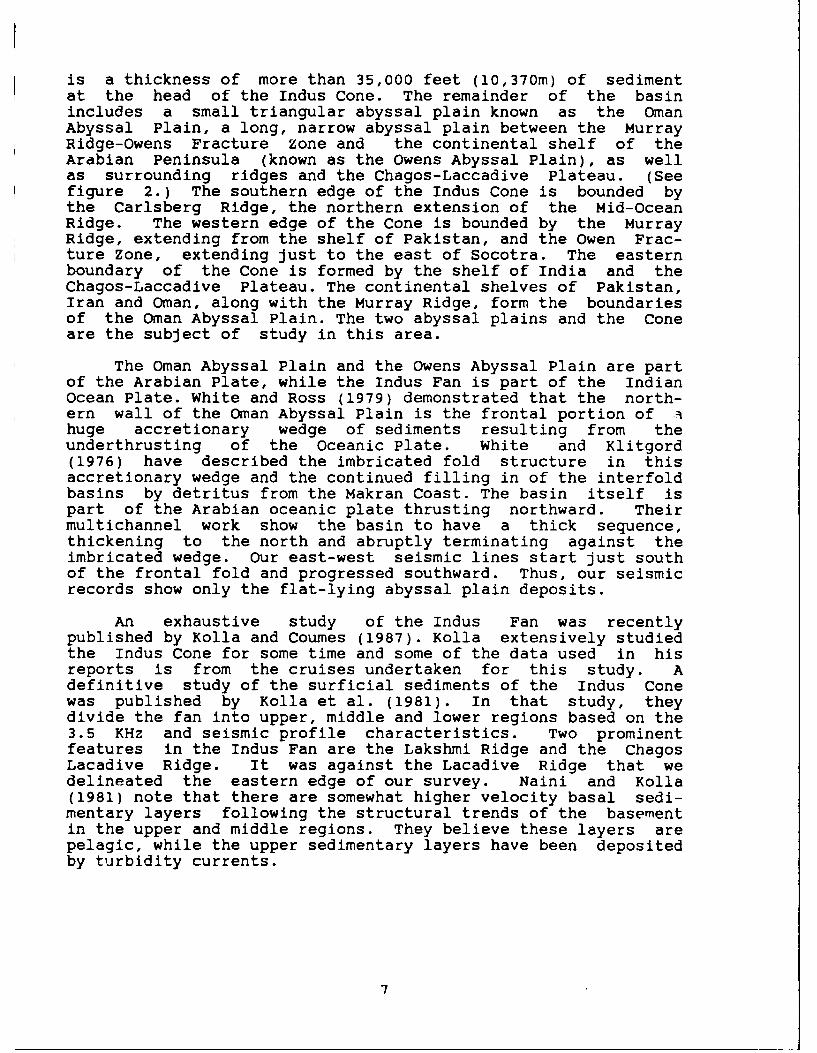
is a thickness of more than 35,000 feet (10,370m) of sedimentat the head of the Indus Cone. The remainder of the basinincludes a small triangular abyssal plain known as the OmanAbyssal Plain, a long, narrow abyssal plain between the MurrayRidge-Owens Fracture zone and the continental shelf of theArabian Peninsula (known as the Owens Abyssal Plain), as wellas surrounding ridges and the Chagos-Laccadive Plateau. (Seefigure 2.) The southern edge of the Indus Cone is bounded bythe Carlsberg Ridge, the northern extension of the Mid-OceanRidge. The western edge of the Cone is bounded by the MurrayRidge, extending from the shelf of Pakistan, and the Owen Frac-ture Zone, extending just to the east of Socotra. The easternboundary of the Cone is formed by the shelf of India and theChagos-Laccadive Plateau. The continental shelves of Pakistan,Iran and Oman, along with the Murray Ridge, form the boundariesof the Oman Abyssal Plain. The two abyssal plains and the Coneare the subject of study in this area.
The Oman Abyssal Plain and the Owens Abyssal Plain are partof the Arabian Plate, while the Indus Fan is part of the IndianOcean Plate. White and Ross (1979) demonstrated that the north-ern wall of the Oman Abyssal Plain is the frontal portion of Ahuge accretionary wedge of sediments resulting from theunderthrusting of the Oceanic Plate. White and Klitgord(1976) have described the imbricated fold structure in thisaccretionary wedge and the continued filling in of the interfoldbasins by detritus from the Makran Coast. The basin itself ispart of the Arabian oceanic plate thrusting northward. Theirmultichannel work show the basin to have a thick sequence,thickening to the north and abruptly terminating against theimbricated wedge. Our east-west seismic lines start just southof the frontal fold and progressed southward. Thus, our seismicrecords show only the flat-lying abyssal plain deposits.
An exhaustive study of the Indus Fan was recentlypublished by Kolla and Coumes (1987). Kolla extensively studiedthe Indus Cone for some time and some of the data used in hisreports is from the cruises undertaken for this study. Adefinitive study of the surficial sediments of the Indus Conewas published by Kolla et al. (1981). In that study, theydivide the fan into upper, middle and lower regions based on the3.5 KHz and seismic profile characteristics. Two prominentfeatures in the Indus Fan are the Lakshmi Ridge and the ChagosLacadive Ridge. It was against the Lacadive Ridge that wedelineated the eastern edge of our survey. Naini and Kolla(1981) note that there are somewhat higher velocity basal sedi-mentary layers following the structural trends of the basementin the upper and middle regions. They believe these layers arepelagic, while the upper sedimentary layers have been depositedby turbidity currents.
7
I. INSTRUMENTATION FOR DATA COLLECTION
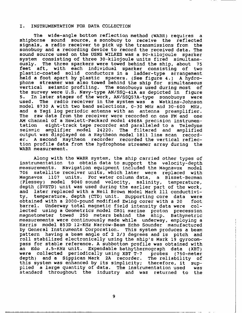
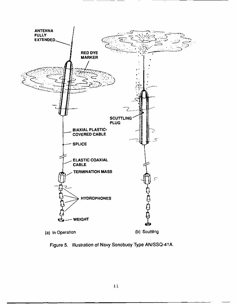
The wide-angle bottom reflection method (WABR) requires ashipborne sound source, a sonobuoy to receive the reflectedsignals, a radio receiver to pick up the transmissions from thesonobuoy and a recording device to record the received data. Thesound source used on the USNS WILKES was a 90-kilojoule sparkersystem consisting of three 30-kilojoule units fired simultane-ously. The three sparkers were towed behind the ship, about 75feet aft, with each individual sparker consisting of twoplastic-coated solid conductors in a ladder-type arrangementheld a foot apart by plastic spacers. (See figure 4.) A hydro-phone streamer was also towed behind the ship for simultaneousvertical seismic profiling. The sonobuoys used during most ofthe survey were U.S. Navy-type AN/SSQ-41A as depicted in figure5. In later stages of the work, AN/SSQ57A-type sonobuoys wereused. The radio receiver in the system was a Watkins-Johnsonmodel 8730 A with two band selections, 0-30 MHz and 30-600 MHz,and a Yagi log periodic antenna with an antenna preamplifier.The raw data from the receiver were recorded on one FM and oneAM channel of a Hewlett-Packard model 4968A precision instrumen-tation eight-track tape recorder and paralleled to a Teledyneseismic amplifier model 24220. The filtered and amplifiedoutput was displayed on a Raytheon model 1811 line scan record-er. A second Raytheon recorder recorded the vertical reflec-tion profile data from the hydrophone streamer array during theWABR measurement.
Along with the WABR system, the ship carried other types ofinstrumentation to obtain data to support the velocity-depthmeasurements. Navigation equipment included the Magnavox model706 satellite receiver units, which later were replaced withMagnavox 1107 units. For water column data, a Bisset-Berman(Plessey) model 9040 sound velocity, salinity, temperature,depth (SVSTD) unit was used during the earlier part of the work,and later replaced with a Neil Brown Model Mark 111 conductivi-ty, temperature, depth (CTD) unit. Supporting core data wereobtained with a 2000-pound modified Ewing corer with a 20 footbarrel. Underway total magnetic field intensity data were col-lected using a Geometrics model G801 marine proton precessionmagnetometer towed 250 meters behind the ship. Bathymetricmeasurements were continuously made while underway, employing aHarris model 853D 12-KHz Narrow-Beam Echo Sounder manufacturedby General Instruments Corporation. This system produces a beampattern having a beam angle of 2 2/3 degrees and is pitch androll stabilized electronically using the ship's Mark 19 gyrocom-pass for stable reference. A subbottom profile was obtained withan Edo 3.5-KHz unit. Expendable bathythermograph data (XBT)were collected periodically using XBT T-7 probes (750-meterdepth) and a Sippican Mark 2A recorder. The reliability ofthis system was enhanced by its simplicity; therefore, it sup-plied a large quantity of data. The instrumentation used wasstandard throughout the industry and was returned to the
9

NOBUOUII
S-SPARKER
(a) Illustration of Both Vertical Profiling and Wide-Angle Bottom Reflection.I
ANTENNA '•7< < "I
SONOBUOY
I TRIGER • PROFILE
•,RECORDERI
BANK
I
(b) Block Diagram of a Typical System.
Figure 4. Illustration th Versmca Profiin adieiling System. R
I
•o I
ANTENNAFULLY j'- -5EXTENDED~ I
RED DYEMARKER
SCUTTLINGPLUG
BIAXIAL PLASTIC- -
COVERED CABLE
-SPLICE
ELASTIC COAXIALCCABLE
TTERMINATION MASSL'-
HYDROPHONES
-- WEIGHT
(a) In Operation (b) Scuttling
Figure 5. Illustration of Navy Sonobuoy Type AN/SSQ-41A.
11
I
manufacturer or to NAVOCEANO laboratories periodically for cali-bration and maintenance. A rigorous preventative maintenanceprogram was carried on aboard the ship and the calibration ofthe instruments checked prior to each cruise. Most sonobuoysdo not transmit true amplitudes and since travel times are theprimary consideration in this study rather than amplitudes, theaccuracy of the timing systems of the recorders is of primeimportance. The recorders are controlled by crystal oscillatorswith an accuracy of five parts per million, and these weremonitored by two rubidium frequency standards aboard the ship.
Data are easily reproducible from the raw data on magnetic Itape, from the original visible recordings or from the 35-mmfilm copies made of all of the seismic records. The intervalvelocities and the thicknesses obtained for each station by theDix (1955) method have been tabulated and are being publishedas a NAVOCEANO Basic Data Report. This publication will includeall of the stations taken through 1988.
IIIIIIIIIII
II. DATA ACQUISITION AND PROCESSING
Several other methods of obtaining seismic velocity datawere considered for this study. The two-ship wide-aperturemethod was evaluated but was discarded due to the costsinvolved and the difficulty of obtaining two ships for a projectover such large areas and requiring so much ship time. Multi-channel reflection methods are highly desired for the increaseddetail and the much greater discrimination of layer thicknesses,but the level of effort and costs of using this method werebeyond the means of the project. Also, since the bulk of thework was in water depths greater than 3000 meters, the workwas beyond the capabilities of the average multi-channel system.Refraction methods would have been as suitable as the WABRmethod as far as costs and ship time were concerned, but therequirement of large sources rich in low frequencies necessi-tates explosives, giving rise to a myriad of regulations andconditions aboard Navy ships. The availability of sonobuoys atminimal cost to NAVOCEANO and the need for only one ship madeWABR the method of choice.
The data used for the characterization of the two oceanareas were acquired over a period from 1979 to 1985 andrequired nine cruise legs for the task. Cruise legs were multi-disciplinary and the tracks were planned to accommodate otherdisciplines, yet have the opportunity to take measurements in asystematic manner so that stations would be located to takeadvantage of physiography. Wide-angle reflection measurementswere the primary purpose of the cruises in the Arabian Sea andthe tracks were designed specifically for this purpose. Aseries of tracks was chosen to obtain uniform coverage of theregion while maintaining tracks along depth contours to minimizethe variation in water depth along the track.
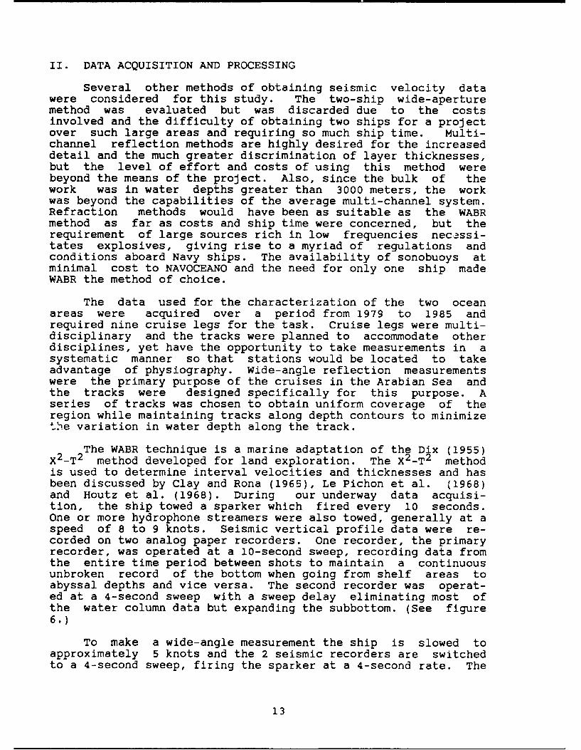
The WABR technique is a marine adaptation of the Dix (1955)X2 -T 2 method developed for land exploration. The X2 -T 2 methodis used to determine interval velocities and thicknesses and hasbeen discussed by Clay and Rona (1965), Le Pichon et al. (1968)and Houtz et al. (1968). During our underway data acquisi-tion, the ship towed a sparker which fired every 10 seconds.One or more hydrophone streamers were also towed, generally at aspeed of 8 to 9 knots. Seismic vertical profile data were re-corded on two analog paper recorders. One recorder, the primaryrecorder, was operated at a 10-second sweep, recording data fromthe entire time period between shots to maintain a continuousunbroken record of the bottom when going from shelf areas toabyssal depths and vice versa. The second recorder was operat-ed at a 4-second sweep with a sweep delay eliminating most ofthe water column data but expanding the subbottom. (See figure6.)
To make a wide-angle measurement the ship is slowed toapproximately 5 knots and the 2 seismic recorders are switchedto a 4-second sweep, firing the sparker at a 4-second rate. The
13
U-U0
Cc91*
00
uJu
C,.
CnC
00Uo C.
wSN3S MR13V I AY0)M
C,, C14
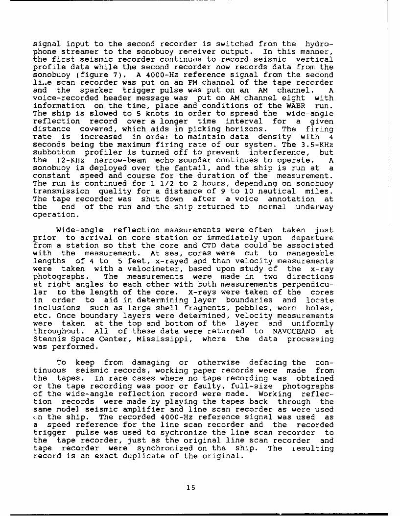
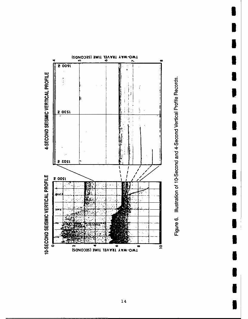
signal input to the second recorder is switched from the hydro-phone streamer to the sonobuoy receiver output. In this manner,the first seismic recorder continues to record seismic verticalprofile data while the second recorder now records data from thesonobuoy (figure 7). A 4000-Hz reference signal from the secondli.,e scan recorder was put on an FM channel of the tape recorderand the sparker trigger pulse was put on an AM channel. Avoice-recorded header message was put on AM channel eight withinformation on the time, place and conditions of the WABR run.The ship is slowed to 5 knots in order to spread the wide-anglereflection record over a longer time interval for a givendistance covered, which aids in picking horizons. The firingrate is increased in order to maintain data density with 4seconds being the maximum firing rate of our system. The 3.5-KHzsubbottom profiler is turned off to prevent interference, butthe 12-KHz narrow-beam echo sounder cnntinues to operate. Asonobuoy is deployed over the fantail, and the ship is run at aconstant speed and course for the duration of the measurement.The run is continued for 1 1/2 to 2 hours, depending on sonobuoytransmission quality for a distance of 9 to 10 nautical miles.The tape recorder was shut down after a voice annotation atthe end of the run and the ship returned to normal underwayoperation.
wide-angle reflection measurements were often taken justprior to arrival on core station or immediately upon departurefrom a station so that the core and CTD data could be associatedwith the measurement. At sea, cores were cut to manageablelengths of 4 to 5 feet, x-rayed and then velocity measurementswere taken with a velocimeter, based upon study of the x-rayphotographs. The measurements were made in two directionsat right angles to each other with both measurements perpendicu-lar to the length of the core. X-rays were taken of the coresin order to aid in determining layer boundaries and locateinclusions such as large shell fragments, pebbles, worm holes,etc. Once boundary layers were determined, velocity measurementswere taken at the top and bottom of the layer and uniformlythroughout. All of these data were returned to NAVOCEANO atStennis Space Center, Mississippi, where the data processingwas performed.
To keep from damaging or otherwise defacing the con-tinuous seismic records, working paper records were made fromthe tapes. In rare cases where no tape recording was obtainedor the tape recording was poor or faulty, full-size photographsof the wide-angle reflection record were made. Working reflec-tion records were made by playing the tapes back through thesame model seismic amplifier and line scan recorder as were usedun the ship. The recorded 4000-Hz reference signal was used asa speed reference for the line scan recorder and the recordedtrigger pulse was used to sychronize the line scan recorder tothe tape recorder, just as the original line scan recorder andtape recorder were synchronized on the ship. The iesultingrecord is an exact duplicate of the original.
15
qr(saNo33S) 3WAI1 13AVW. AVM-OMJ.
In co
00
00
00
ImILLI (D3
F~oCIU)I: 1:10
cu
i u
1F, zo -I,'I
U-U
zoos L jIIn to
(saNo03S) 3YUI 13AV81 AVM-OMIL
16
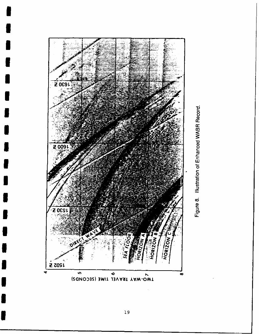
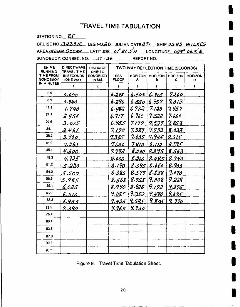
iProcessing to obtain velocities was done as follows: Using
the seismic vertical profile record made during the station,coherent reflections were picked out and transferred to theworking record. The trace of the direct wave and the trace ofthe arrivals from the reflections were enhanced with colorpencil as shown in figure 8. Travel times of the direct waveand each of the reflected arrivals were measured from the recordand tabulated on a form as illustrated in figure 9. The near-surface water sound velocity, at the sparker depth and thesonobuoy hydrophone depth, was obtained from CTD data and usedto calculate the distance from source to receiver based on theI. direct wave travel time. These data were input to a computerprogram written by Michael McGlaughlin of NAVOCEANO and lateri slightly modified by the author. (See appendix C.)
The program calculates the squares of the arrival times anddistances, and uses the least-suuares method to fit the beststraight line to the plotted XL-T2 values. A coefficient ofcorrelation (COC) calculated to determine the degree of fit wasalso found useful in determining "picking" errors and numericaltranspositions in entering the data into the computer. TheI correlation coefficient is defined as "the square root ofthe ratio of the explained variation to the total variation."It is a measure of the goodness of fit between the assumedequation and the data. If the Dix conditions of horizontal andparallel layers are met, the plot of the X2 -T 2 values is astraight line. The correlation coefficient would then be 1.0,and lower values indicate that either the conditions were notI met or there are errors or noise in the data set. No fit ofmore than two data points is ever perfect; however, exceptional-ly good fits will achieve a COC of 0.99997 or 0.99998. As anexample, an error of 0.2 seconds in arrival time will affect thefourth decimal place and result in a coefficient of 0.9996 or0.9997. Checking the poor correlation coefficients most oftenresulted in detecting errors in picking travel times or transpo-sition errors. Poor course 2maintenance or variations in speedshow up as waves in the X -T plot or bunching up of the datapoints. A disconcerting characteristic of our computer plottingroutines is that COCs are rounded off at the fifth decimalplace, thus resulting in coefficients of 1.0.
3- After establishing the straight line fit, the computerprogram then goes through the Dix calculations and determinesinterval velqci~ies and interval thicknesses. The programi outputs the XZ-T plot and a tabulation of the input data withthe resulting interval velocities and thicknesses as shown infigures 10 and 11. As noted earlier, the correlation coeffi-cients indicated as 1.0000 in figure 11 have been rounded off atthe fifth decimal and are actually on the order of 0.99998.
The velocimeter measurements made at sea are later correct-ed for temperature and pressure at NAVOCEANO's core lab. Theprocedure used for making the corrections is included asappendix B. The measurements for each core were averaged over a
i 17
idepth interval of 30 centimeters. In the tabulation of station Ulayer thicknesses and layer velocities, the initial thickness(0.000) and associated velocity is that obtained from the coreanalysis.
3U
IiUU
IUU
Iii
18 3
.....I.
IzO9L;Z
1c
IC2 4 009L
3 jfl"t"IJY~44LJ
C6
U~ ~ ý O-C&iS*'ILIW
4'4
0 19
1TRAVEL TIME TABULATION 1
STATION NO. &A-
CRUISE NO..3At37/L6 . LEG NO.ai_ JULIAN DATE.?7/_ SHIP u1 M5 WiL-E3 1AREAND1AN OCEAN LATITUDE 0/i /,SA LONGITUDE 3V9*06 .JIE
SONOBUOY: CONSEC. NO. .-30- 3 REPORT NO.__
SHIP'S DIRECTWAVE DISTANCE TWO-WAY REFLECTION TIME (SECONDS)RUNNING TRAVEL TIME SHIPTO
TIME FROM IN SECONDS SONOBUOY SEA HORIZON HORIZON HORIZON HORIZONSONOBUOY (ONE-WAY) IN KM. FLOOR A B C DIN MINUTES t
0.0 , •;•3 L7&5 7.2"• o8.5 _ 6,29 6.To 6.971 7.313
17.1 6.€€ .yfc 41¢32 7/126 '7.. 57
24.1 4,.71.7 L ?s 7.,3= Z?6•29.6 63,51s.- A / 7 7,5Z7 7.,Z "134 .1 __ 7. 7.Z3,9? 7,33 ' .63.38.2 3 _ _as 9L91s41.9 _.Q s 7, 10 7J9/0 , 1 3 , -f45.1 V49o 67d 000 9AM _ U51.2 9.% 9,2S g. 66 -9, ?S1 _
54.0 9-311 9J.s. 9 d._7, _,_
56.6 _ _, 79U g,,.g 9.2s. 706 ?•, 2 _
59.1 o ___ ,47Y69, V9_/_7,7__ I63.9 5-9 9__1~&L ~ Y~~~
72.5 _9,' Y7-_76.480.1
83.6
87.0
90.3 393.5
Figure 9. Travel lime Tabulation Sheet.
20 3
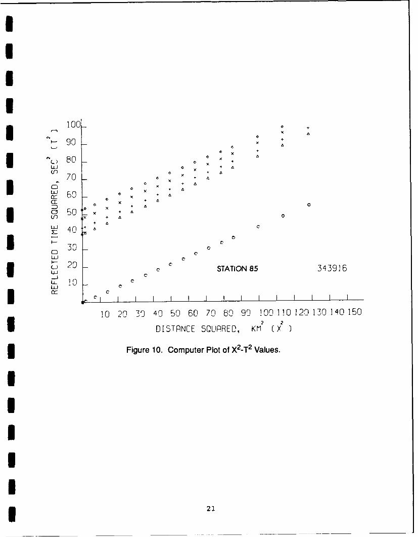
IO
100- +
x
+
x +80 x +
Li + bn(f). 0
70 x ++ + e
oLJ 60 + nCE xD 0 +
L x + ,+I 40 °30o
F-i
_20 STATION 85 34 3916
LIC--
i-- lI I I ! J ! I I I I It
10 20 30 40 50 60 70 80 90 !00 110 120 170 140 150
SDISTANCE SOLIPRED, KM (X X
3 Figure 10. Computer Plot of X2-T2 Values.
i
i
I
I
I

z
0 M 0000a0 0 0 00 000000 CC
OC0 0000C00000000
U 000000 C000000 00000
.0 0 O o o O ~ ~ ~ ~0 a 4 - 0
O00o00cooo 000
D -00.000000000000000
0 10 Ln a. %A pn Q P. p- O0 CDtl 00 x rv ar.0 CC pn n f -C v n'a0ft0
0 ýmCI kna I 0.0.0.0P-NP-0.Qe O0
tJ kn CC -o 0 ry to.,u w.lOw fl D0 NM .eN M al.0: 40.0a,
z .1 .
N wf Q . f N 0 P i n 0 f ' O O 0 0 a c
01 - .00,c n r. ~ 0 M0, PM& .eftA'r. *on
0- w 0.
U~F 0 N
0 ~ ~ ~ ~ ~ 1 F. 2 O BN N W .O O O 0
0 n wU m
O9ftOQM 0n ft7ft "A00%.
If n atP.0 .- 0 O N
M0NA0V, 'D 0 0 U P.-Q .A *,V 0
WC) P-a M. 0-C!O PZ000.' 0.. D p.. - ý g. Z n" .i
ft f 0' BA 0 40 BA m I
N EJO m W
W) .~ 0 ta ,0O
03 0' ft0Q F; 0 w 0'
Q Ij1 CalN 0-M0 0310-0 N
BA~OF &A 0 vN O u =N't P!aA AU 3No Nc -v -wr A l-
7O 6n 0, c j ~I0 z .
f. P4 W- aM a~ aW r. wl '0.0 .0 NbPNa.-M.0 3 b~N Na.4
223
III. DATA INTERPRETATION
The WABR method estimates a velocity versus depthrelationship where the depth is expressed in terms of layerthickness and the velocity is an average velocity for the layer.Investigators in this area prefer to express this as aparameterized relationship in terms of velocity versus one-waytravel time, called an instantaneous velocity function. Acous-tic modelers prefer to work in terms of velocity versus depth.Thus, after obtaining the interval velocities and thicknessesfor each of the WABR measurements, as described in the sectionon data acquisition and processing, the next step is to deriveinstantaneous velocity curves for each station. This isaccomplished by making plots of the interval velocity dataversus one-way travel time from the sediment surface to themidpoint of the interval. A curve is then fit to the plotteddata points. This method was discussed by Houtz et al. (1968,I 1970), Hamilton et al. (1974) and Bachman and Hamilton (1980)and was closely followed in this work.
As noted by these authors, interval velocity measurementshave the drawback of modeling reality as constant velocitylayers, thus yielding first-order discontinuities that may notexist, leading to erroneous reflection coefficients. Hamiltonet al. (1974) and Bachman and Hamilton (1980) have pointedout the importance of sediment surface velocities to theacoustic community and how these data provide anchor points inthe velocity versus one-way travel time plot. To provide thesedata in this study, sediment surface velocities were obtainedfrom cores as noted earlier.
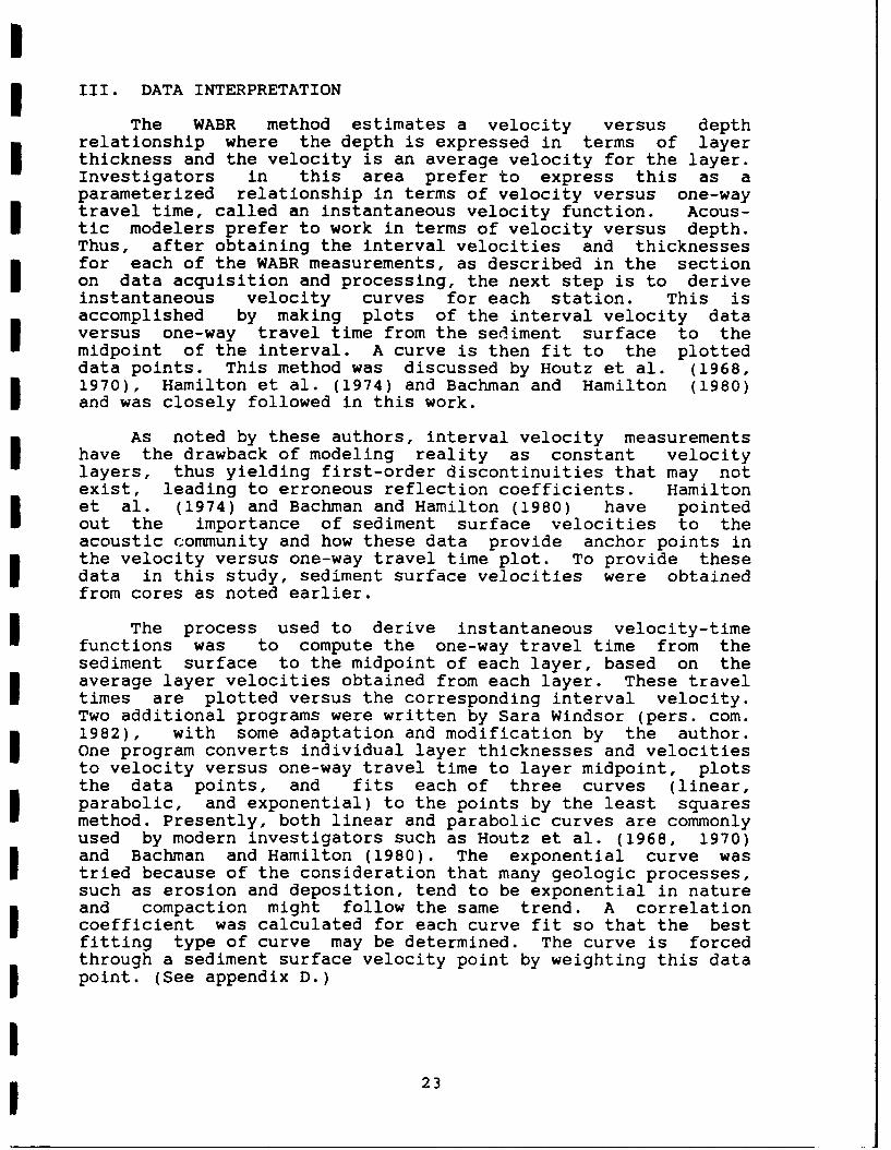
The process used to derive instantaneous velocity-timefunctions was to compute the one-way travel time from thesediment surface to the midpoint of each layer, based on theaverage layer velocities obtained from each layer. These traveltimes are plotted versus the corresponding interval velocity.Two additional programs were written by Sara Windsor (pers. com.1982), with some adaptation and modification by the author.One program converts individual layer thicknesses and velocitiesto velocity versus one-way travel time to layer midpoint, plotsthe data points, and fits each of three curves (linear,parabolic, and exponential) to the points by the least squaresmethod. Presently, both linear and parabolic curves are commonlyused by modern investigators such as Houtz et al. (1968, 1970)and Bachman and Hamilton (1980). The exponential curve wastried because of the consideration that many geologic processes,such as erosion and deposition, tend to be exponential in natureand compaction might follow the same trend. A correlationcoefficient was calculated for each curve fit so that the bestfitting type of curve may be determined. The curve is forcedthrough a sediment surface velocity point by weighting this datapoint. (See appendix D.)
23

IIn the second program, data from several stations are then
combined on the same graph and again fit with each of thethree different curves and correlation coefficients calculat-ed. Each curve is forced through the average surface sedimentvelocity of all of the stations included in the run. (See appen- Ddix E.) It should be noted that in spite of heavy weighting ofthe surface velocity data point, the best fit curve oftenresulted in a slightly different surface velocity due to skew-ing of the line or curve by the remaining data points. Theauthor felt that this was acceptable, even though the surfacevelocity is a directly measured quantity because of the possibleerrors involved in the core sample velocity measurements and areasonable validity given to the other data points. An exampleof a single station plot and a group station plot is given infigure 12. I
Of the 70 stations in the Somali Basin, 80% of the velocityversus one-way time data were best fit by a parabolic curveand the remaining 20% were best fit by a linear curve. Thecriteria for fit was the correlation coefficient. The coeffi-cient of correlation is a measure of how well a linear or otherequation describes the relationship between the variables. A ICOC of 1.0 is a perfect fit. Of those stations best fit by aparabolic curve, the difference in the correlation coefficientsbetween parabolic and linear fit was at the most 0.01 and mostoften on the order of 0.005. Thus, it would be reasonableto assume a linear function for one-way travel time plots forthe areas investigated. The exponential curve was the best fitby correlation coefficient in only one case out of all cases,and it was thus assumed that the speculation concerning theexponential nature of compaction was not justified.
Plotting the interval velocity at the midpoint of the layeris valid only if the layer has a constant velocity or if thevelocity increases linearly with depth. If the best curve fitis parabolic, then the linear conditions are not met and theposition in the layer at which the interval velocity is assignedmust be corrected. Houtz et al. (1968) made an analysis ofthe error involved in placing the interval velocity at thelayer midpoint when the velocity increases in the layer as asecond-order function. The error analysis determines that thecorrection for the interval velocity position in the layer is UE = Cdt /12, whIre C is the constant in the parabolic curve fitgiven by V = At +Bt+C and dt is the interval thickness in termsof one-way travel time. Thus, when the correlation coefficientindicates that the best fit is the parabolic curve, the positionof the interval velocity in the layer is corrected by the factorE, replotted and refit with a parabolic curve for the resultant"Instantaneous Velocity Curve" of Houtz et al. (1968) and Hamil- Iton et al. (1974). An example of instantaneous velocity curvesderived using data from one station and data from numerousstations is presented in figure 12. i
I
C CD
ux oc c r
Li C) CD -)( a: C)
Li 'a Lz S rý z-
Ui C L) C:t-J
Ii - - L - u:-LL.0 L.3 Li L
Li ~ -' -s C - -
C) cc l U C) a i~
>C C) - C) - m
Ci)U ) C
Li (1- 0 ) C ' C -C
9-Li a: Li M) Liý
cr r~ Of 0
0Sý3c N I:ýW!I -1AUýý IUM3NO ...
CC
C/)
CL
0
CD .1Ir CU x c
CD Ir (r a: mr
Li X9L Li I
I- - : r~i a-z z x Z
M/ Li i)LLi L - - - - - :3Li -C- K )C
-1 9 L- r'N L- -L -Li Li + Li 0)
C) I C) I C)L) C) ui - . L.; C) U-
m) -1 / r x a)0 2 C) C : C
7- o:-. mT
ae ) C) L: C- CD
L) L ) m L.) C)- U< C)
S3~N! :3w~ 13AY~.L ;OM* JNO
25
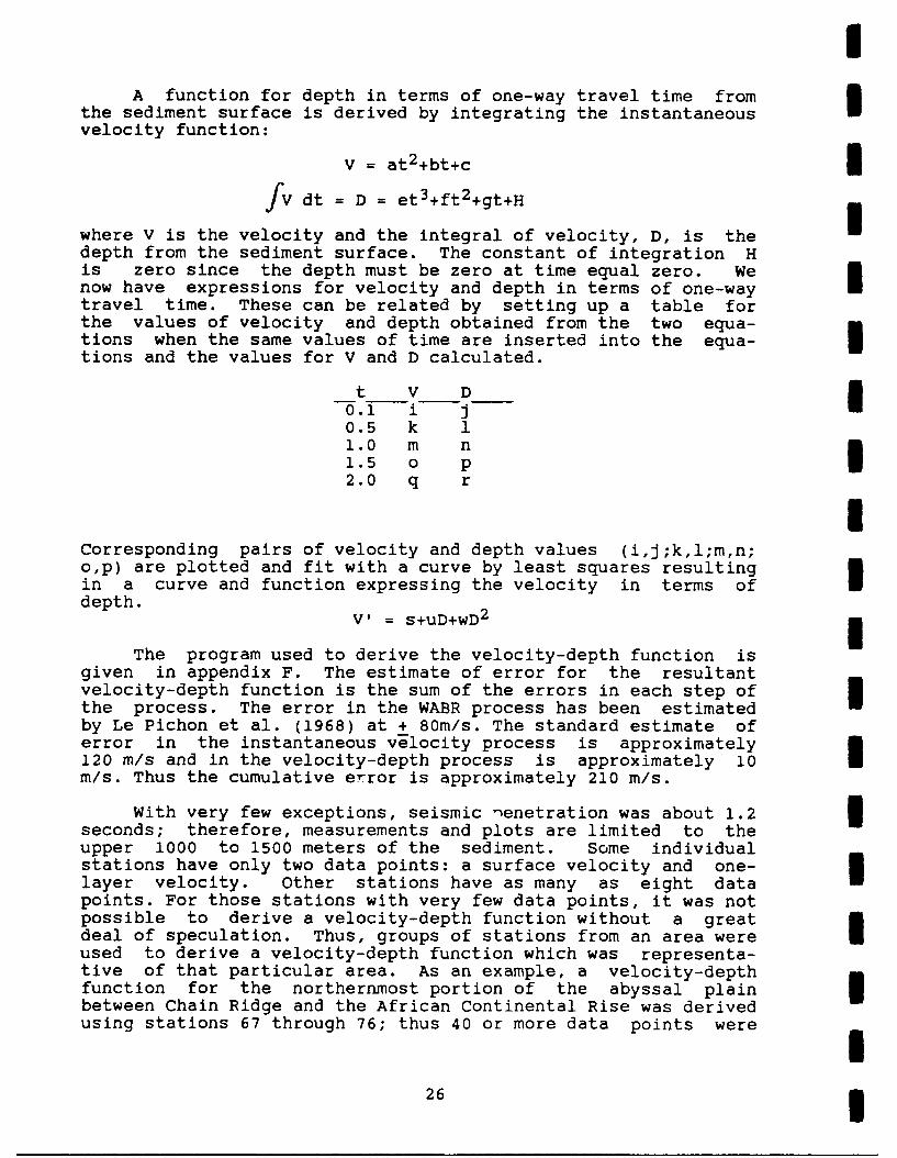
IA function for depth in terms of one-way travel time fromthe sediment surface is derived by integrating the instantaneous
velocity function:
V = at 2 +bt+c
fv dt = D =et3+ft2+gt+H
where V is the velocity and the integral of velocity, D, is thedepth from the sediment surface. The constant of integration His zero since the depth must be zero at time equal zero. Wenow have expressions for velocity and depth in terms of one-waytravel time. These can be related by setting up a table forthe values of velocity and depth obtained from the two equa-tions when the same values of time are inserted into the equa- Itions and the values for V and D calculated.
t V D0.i i I0.5 k 11.0 m n1.5 o p U2.0 q r I
Corresponding pairs of velocity and depth values (i,j;k,l;m,n;o,p) are plotted and fit with a curve by least squares resultingin a curve and function expressing the velocity in terms of Udepth. V' = s+uD+wD2
The program used to derive the velocity-depth function isgiven in appendix F. The estimate of error for the resultantvelocity-depth function is the sum of the errors in each step ofthe process. The error in the WABR process has been estimatedby Le Pichon et al. (1968) at + 80m/s. The standard estimate oferror in the instantaneous velocity process is approximately120 m/s and in the velocity-depth process is approximately 10m/s. Thus the cumulative error is approximately 210 m/s.
With very few exceptions, seismic "enetration was about 1.2 3seconds; therefore, measurements and plots are limited to theupper 1000 to 1500 meters of the sediment. Some individualstations have only two data points: a surface velocity and one-layer velocity. Other stations have as many as eight datapoints. For those stations with very few data points, it was notpossible to derive a velocity-depth function without a greatdeal of speculation. Thus, groups of stations from an area wereused to derive a velocity-depth function which was representa-tive of that particular area. As an example, a velocity-depthfunction for the northernmost portion of the abyssal plain Ibetween Chain Ridge and the African Continental Rise was derivedusing stations 67 through 76; thus 40 or more data points were
263
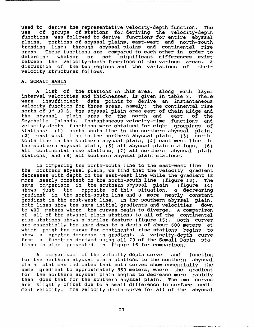
used to derive the representative velocity-depth function. Theuse of groups of stations for deriving the velocity-depthfunctions was followed to derive functions for entire abyssalplains, portions of abyssal plains, east-west and north-southtrending lines through abyssal plains and continental riseareas. These functions are compared to each other in order todetermine whether or not significant differences existbetween the velocity-depth functions of the various areas. Adiscussion of the two regions and the variations of theirvelocity structures follows.
A. SOMALI BASIN
A list of the stations in this area, along with layerinterval velocities and thicknesses, is given in table 3. Therewere insufficient data points to derive an instantaneousvelocity function for three areas, namely: the continental risenorth of 30 30'S, the abyssal plain area east of Chain Ridge andthe abyssal plain area to the north and east of theSeychelle Islands. Instantaneous velocity-time functions andvelocity-depth functions were obtained for eight groupings ofstations: (1) north-south line in the northern abyssal plain,(2) east-west line in the northern abyssal plain, (3) north-south line in the southern abyssal plain, (4) east-west line inthe southern abyssal plain, (5) all abyssal plain stations, (6)all continental rise stations, (7) all northern abyssal plainstations, and (8) all southern abyssal plain stations.
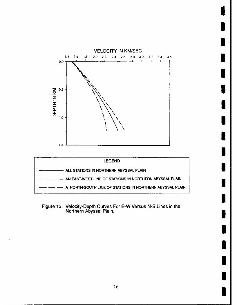
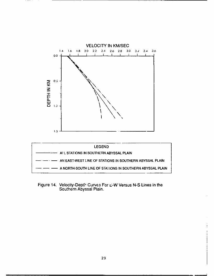
In comparing the north-south line to the east-west line inthe northern abyssal plain, we find that the velocity gradientdecreases with depth on the east-west line while the gradient ismore nearly constant on the north-south line (figure 13). Thesame comparison in the southern abyssal plain (figure 14)shows just the opposite of this situation, a decreasinggradient in the north-south line and a more nearly constantgradient in the east-west line. In the southern abyssal plain,both lines show the same initial gradients and velocities downto 400 meters where the curves begin to diverge. A comparisonof all of the abyssal plain stations to all of the continentalrise stations shows a similar feature (figure 15). Both curvesare essentially the same down to a depth of about 600 meters atwhich point the curve for continental rise stations begins toshow a greater decrease in gradient. A velocity-depth curvefrom a function derived using all 70 of the Somali Basin sta-tions is also presented in figure 15 for comparison.
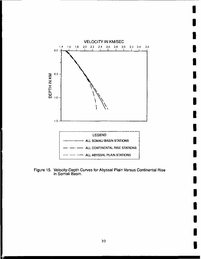
A comparison of the velocity-depth curve and functionfor the northern abyssal plain stations to the southern abyssalplain stations indicates that both curves show essentially thesame gradient to approximately 350 meters, where the gradientfor the northern abyssal plain begins to decrease more rapidlythan does that for the southern abyssal plain. The two curvesare slightly offset due to a small difference in surface sedi-ment velocity. The velocity-depth curve for all of the abyssal
27
III
VELOCITY IN KM/SEC1.4 1 1.8 2.0 2.2 2.4 2.6 2.8 3.0 3.2 3.4 3.6 3
0.0
0.5\
z=
1.0 3
1.5
LEGEND
ALL STATIONS IN NORTHERN ABYSSAL PLAINI
- -- AN EAST-WEST LINE OF STATIONS IN NORTHERN ABYSSAL PLAIN
- -- A NORTH-SOUTH LINE OF STATIONS IN NORTHERN ABYSSAL PLAIN
Figure 13. Velocity-Depth Curves For E-W Versus N-S Lines in theNorthern Abyssal Plain.3
I
1.28
VELOCITY IN KM/SEC1.4 1.6 1.8 2.0 2.2 2.4 2.6 2.8 3.0 3.2 3.4 3.6
0.0 -
0.5
z
0,
S1.0
1.5-
LEGEND
Al L STATIONS IN SOUTHERN ABYSSAL PLAIN
AN EAST-WEST LINE OF STATIONS IN SOUTHERN ABYSSAL PLAIN
A NORTH-SOUTH LINE OF STATIONS IN SOUTHERN ABYSSAL PLAIN
Figure 14. Velocity-Depth Curves For E-W Versus N-S Lines in theSouthern Abyssal Plain.
29
III
VELOCITY IN KM/SEC1.4 1.6 1.8 2.0 2.2 2.4 2.6 2.8 3.0 3.2 3.4 3.6 3
I0.5- I
z0= I
I.-Qi.o \ \ II
I1.5-
LEGEND
ALL SOMALI BASIN STATIONS
ALL CONTINENTAL RISE STATIONS
ALL ABYSSAL PLAIN STATIONS 3Figure 15. Velocity-Depth Curves for Abyssal Plain Versus Continental Rise I
in Somali Basin.
3IIIIII
30
II plain stations of the Somali Basin is a composite of these two
curves. (See figure 16.) Given that the overall estimate oferror in the velocity-depth curves is of the order of 200 m/s,the differences in the curves presented in figures 13 to 16 isnot much greater than the statistical error. The differences inthe curves are differences in velocity gradient, which dependson factors such as depth, particle size, sorting, sedimenttype, etc. The station group curve is derived from the data ofa number of stations sampling different portions of the basin.Thus, each group curve is the result of an average sampling ofI different portions of the basin which results in variations inthe gradient of the curves.
If a general velocity-depth function for the entire SomaliBasin as an entity is desired, the parabolic function derivedusing all 70 stations would be appropriate; or the simplerlinear function derived from the same data could also be used.A listing of the velocity-depth functions derived for 'his areais given in "section A" of table 1 and a similar listing of theinstantaneous velocity-time functions is given in "section A" ofI table 2.
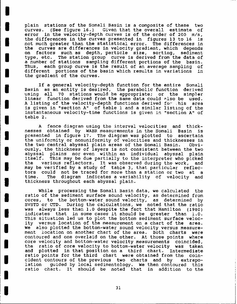
A fence diagram using the interval velocities and thick-nesses obtained by WABR measurements in the Somali Basin ispresented in figure 17. The diagram was plotted to ascertainthe uniformity or nonuniformity of velocities and thicknesses inthe two central abyssal plain areas of the Somali Basin. Obvi-ously, the thickness of layers is not consistent between the twoabyssal plains nor even within an individual abyssal plainitself. This may be due partially to the interpreter who pickedthe various reflectors. It was observed during the work, andmay be verified by a study of table 3, that particular reflec-tors could not be traced for more than a station or two at atime. The diagram indicates a variability of velocity andthickness throughout each abyssal plain.
While processing the Somali Basin data, we calculated theratio of the sediment surface sound velocity, as determined fromcores, to the bottom-water sound velocity, as determined bySVSTD or CTD. During the calculations, we noted that the ratiowas always less than 1.0 despite the fact that Hamilton (1980)indicates that in some cases it should be greater than 1.0.This situation led us to plot the bottom sediment surface veloc-ity versus location of the measurement on a chart of the area.We also plotted the bottom-water sound velocity versus measure-ment iocation on another chart of the area. Both charts werecontoured and one overlaid on the other. At those points wherecore velocity and bottom-water velocity measurements coincided,I the ratio of core velocity to bottom-water velocity was takenand plotted in that position on a third chart. IntermediateI ratio points for the third chart were obtained from the coin-cident contours of the previous two charts and by extrapo-lation guided by local sedimentology. We then contoured thisratio chart. It should be noted that in addition to the
I 31

III
VELOCITY IN KM/SEC1.4 1.6 1.8 2.0 2.2 2.4 2.6 2.8 3.0 3.2 3.4 3.6
0.0-
I
1.5 ILEGEND
ALL ABYSSAL PLAIN STATIONS
- -- ALL STATIONS IN NORTHERN ABYSSAL PLAIN-- ALL STATIONS IN SOUTHERN ABYSSAL PLAIN
Figure 16. Velocity-Depth Curves for Northern Abyssal Plain Versus
Southern Abyssal Plain.32
I!I
010
I
I40- 45* 50. 55°
14- 16K/E10.
40 45 50 55
I
I t
I
I 00 O
I
I 5°-*
F 1int
33s
I ,~. . 4I i .U * 10.I
II0 4S° SO. 5S"5D
Figure 17. Fence Diagram of interval Velocities and Thicknesses in Somali Basin.
III 33
I
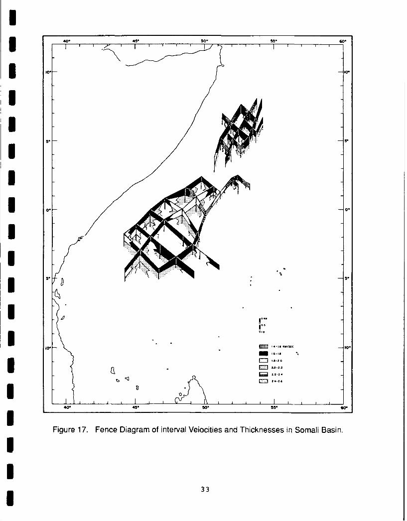
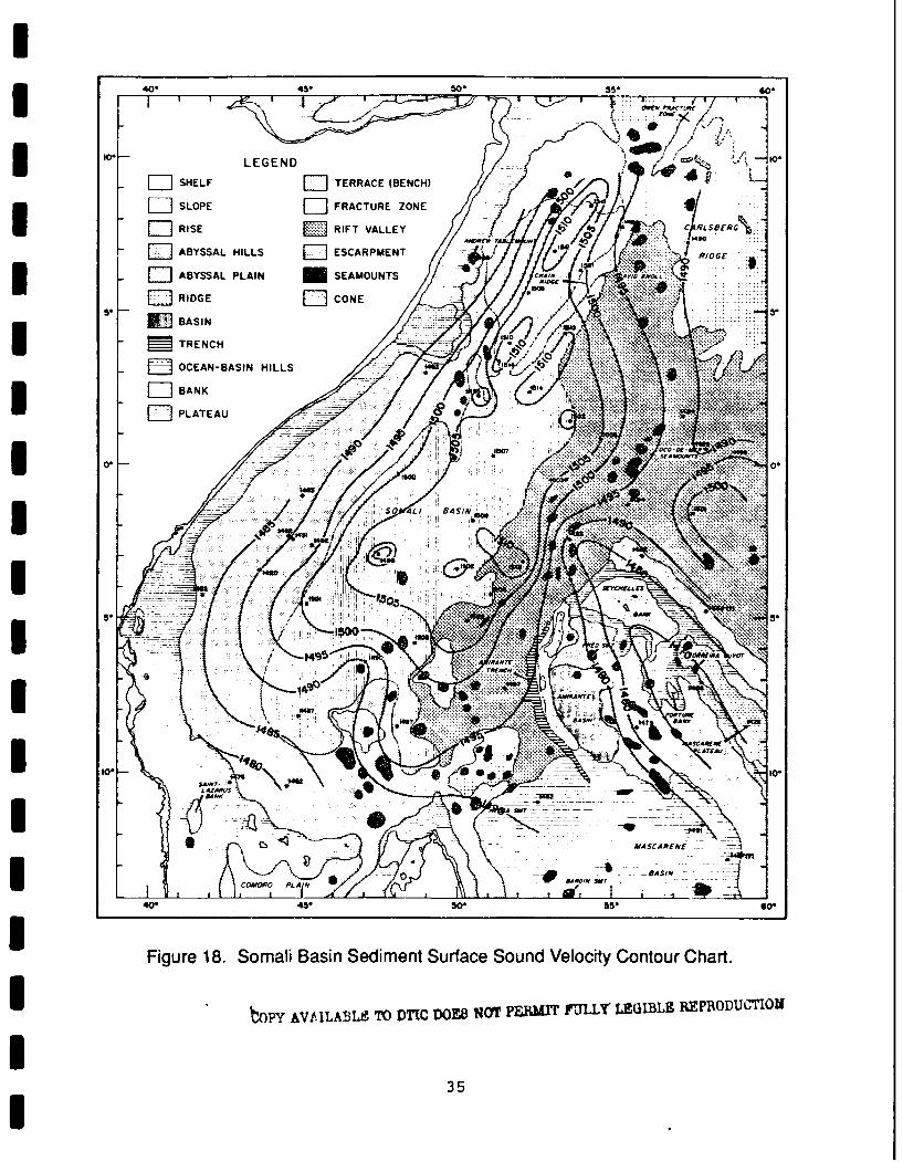
velocities obtained by the USNS WILKES, all available sedimentsurface velocities from the National Oceanographic Data Center Iwere included in the plot. The three plots are presented infigures 18, 19, and 20.
Consideration of figure 18, the contour plot of sedimentsurface velocities, indicates that the sediment surface veloci-ties reflect the bathymetry or physiography to a considerable Iextent. Chain Ridge, though not well defined due to a lack ofvelocity measurements on the Ridge itself, is expressed by ahigh on either side. These highs delineate the abyssal plainson the east and west sides of the Ridge. The sediment surfacevelocities generally increase with ocean depth. Considerationof figure 19, the bottom-water velocity contour chart, shows asexpected (Urick, 1983) that the bottom-water velocity is a Ifunction of depth and therefore controlled by physiography. Inthe northern and eastern portion of the Somali Basin, thebottom-water velocity reflects the physiography to a largedegree. In the western and southern portion of the Basin, thebottom-water velocities are not as high, particularly in theAfrican Continental Rise area and the southernmost portion ofthe abyssal plain area, as those in the northern portion of theBasin, due to the shallower depth. In the southern portion ofthe Basin both sediment surface velocity and bottom-watervelocity do not reflect the physiography nearly as well. IThis situation results in a profound effect on the sedimentsurface velocity/bottom water velocity ratio plot in figure 20.Consideration of this figure indicates that the ratio reflectsphysiography quite well in the northern and east-southeast Iportion of the Basin but has little relationship in the southand west. The ratio contour chart shows a high in the southwestand a low in the south central portion of the basin. This cen- Itral low is the obvious result of the nose of low sedimentvelocities indicated in that area in figure 18. The reason forthe nose of high ratio in the southwest is not apparent when Iconsidering figures 18 and 19.
B. ARABIAN SEA
A list of the stations taken in this area, along with theirinterval velocities and thicknesses, is provided in table 4.
The general process used in this area was the same as thatused in the Somali Basin. An instantaneous velocity-time curvewas obtained for each station taken in the Oman Abyssal Plain.Individual stations were compared to each other to see if therewere anomalous areas. In the Oman Abyssal Plain, it was thoughtthat certain stations might be anomalous on the basis of theirphysiographic location. Stations 131 and 132 were two stationsexpected to be anomalous on the basis of their location in thenortheast corner of the plain where the plain pinches down tosomewhat of a trough. Stations 143, 144, and 145 were expected Ito be anomalous because of. their positions at the extreme southend of the plain where the bottom rises to the Murray Ridge. In
34i
340- 45* so.. Go.
E1SHELF LEED~ TERRACE (BENCH) A
I]SLOPE []FRACTURE ZONE
RISE ~~RIFT VALLEYC LBRN
L]ABYSSAL PILAI EDI ESCARPMENT RIDA'~lGE3BSA LI SEAMOUNTS
15BASIN -
STRENCH WI0 .X :X
E3OCEAN-BASIN HILLS t ...
BANKpl
S BASS,
S COOR BASIN
40~~X 45 5 5*
1 Fiure18. omai Bain edimnt urfae Sund eloity ontur Cart
IW~OY&VLB~ 0DISO ....O...~I UL1 LGBE ERDUTOI&
1495 OW 35
Iý
40* 45* 50* 55 o.
o. LEGENDI
ED SLP E- FRATUE ON
E4 RSEE 48 0 15
BASIN
40* 45* so* 55* 60*
I0* LEGENDISE LII: [ TERRACE (BENCH) -
LIIRISE RIFT VALLEY ~ & .\R S E G
ABYSSAL HILLS El ESAIMETGEI0
I]ABYSSAL PLAIN SEAMOUNTS
[RIDGE LICONE .../.
I ~ TRENCHDOCEAN-BASIN HILLS
WBANK
O PLATEAU .--..- :,,x
I Dan
5. 5. 0 56
Figuren 20 eietSrfc oBto-atrSudVlcty ai otu hr
for th Somal Basin
CAM j37

Ithe analysis, station 124 was found to have a higher gradientthan most of the remainder of the stations, and station 129 wasfound to have a lower gradient. However, both of these stationslacked velocities deeper in the sedimentary section; therefore,the observation may not be significant. Stations 131 and 132 mare very similar to each other and somewhat similar to station
124. Stations 143, 144 and 145 were quite similar to each otherand to the bulk of the stations. i
In a comparison of the instantaneous velocity-time curvesfor each of the stations in the Oman Abyssal Plain, stations124 and 129 were the only stations that seem to be somewhat Ianomalous in their gradients and they were suspect due to theirlack of deeper velocities. Groupings of stations were used tolook for any variations with direction but none were found. The Iend result of the analysis in the Oman Abyssal Plain was thattwo velocity-depth curves were derived for two separate condi-tions: (1) derived using all of the stations except 124 and129, and (2) derived using all of the stations in the AbyssalPlain. There was no difference between the curves. Groups ofstations were plotted together and a velocity-depth curve ob-tained for them. For example, the velocities from stations 124 Ithrough 130 and for stations 133 through 137 were plotted andcurves obtained. The two curves were then compared fordifferences in gradient, etc. The velocities from a group of Istations in a north-south line, stations 128, 134, 139, 141, and145, were similarly plotted and a curve obtained. This curvecould be compared to the curve obtained from stations in aneast-west line. In fact, two north-south lines were run forcomparison to each other and for comparison with an east-westline of stations. This was to detect possible N-S variationwith longitude. I
The group of stations 167 through 170 and 180 and 181 inthe Owens Abyssal Plain which parallels the Arabian Coast wasthen analyzed. These stations are located along the longitudi-nal axis of the plain and were analyzed for variations in thatdirection by comparing individual station velocity-depth curves.No anomalies were detected and all of the station curves weresimilar as expected.
The third group of stations analyzed is that group taken onthe Indus Cone and consisted of stations 146 through 166, 171through 176, 182 through 186, 300 through 312, and 344 through346. The wide grouping of station numbers is due to the factthat various legs were run in different years. The analysis ofthis group of stations was the most varied and also the mostcomprehensive due to the large number of stations and thegeometric pattern of the stations allowing for great variety in ithe analysis. The instantaneous velocity-time curves were usedto determine if there were any anomalous zones in the entirearea. In this initial comparison, stations 146 and 149 are Isomewhat anomalous in that they have slightly higher velocitygradients than other stations. However, both of these stations
i

have only two velocities, a surface velocity and one layervelocity, and are not considered to be very reliable. In com-paring all of the remaining stations, minor differences ininitial velocity and minor differences in gradient are observedbut all of the station curves are remarkably similar. Based onthese results, the stations were arranged in various groupings.For example, all of the stations taken at the nose end of theIndus Cone in water less than 3,000 meters were put into onegroup, all of those in the mid-Cone area in water 3,000 to 4,000meters were put in a second group and all of the stations onthe distal end of the Cone in water 4,000 meters or more wereput in a third group.
Another mode of analysis is to take each line of stationsas a group, 146 through 148 or 149 through 153, and comparethese composite curves to the curve for the adjacent line.Stations are plotted in a stepwise fashion with each line of thetrack down the entire Indus Cone. (See figure 21.) A numberof stations whose positions form a line from north to southacross the Cone are assembled into two groups and compositecurves are derived for stations at different longitudes toevaluate possible variations between the two north-south lines.Two east-west lines of stations were also chosen and curvesobtained to check for variations in curves between east-westlines at different latitudes. Comparisons were made betweenthe north-south lines and east-west lines. Other lines ofstations at various angles around the compass were also used toderive instantaneous velocity-time curves and check for anyradial variations throughout the area.
After all the comparisons and evaluations had beencarried out with all of the various possibilities for groupings,velocity-depth curves were derived for a dozen of the moresignificant groupings. These curves were used for the finalevaluations. Three of the twelve pertained to the Oman AbyssalPlain area and the Owens Abyssal Plain area. Only one veloci-ty-depth function is needed for each of the two abyssal plainareas. The remaining nine velocity-depth functions are derivedfor the Indus Cone area to verify observations from theinstantaneous velocity-time functions. The gradient is suffi-ciently low on the first line of stations (146 through 148) tojustify its own velocity-depth function. All of the remaininglines of stations are found to be similar enough to be modeledby only one velocity-depth function.
Thus, for the Arabian Sea, it is suggested that four sepa-rate velocity-depth functions apply: One for the Oman AbyssalPlain, one for the Owens Abyssal Plain, one for the upperreaches of the Indus Cone (within 160 miles of shore) and onefor the remainder of the Cone. The functions for these fourareas are tabulated in table 1B along with the variance andstandard estimate of error for each function.
39
III
VELOCITY IN KM/SEC
00 2.0 0 .0 0 2.0 0 2.0 "2.0 0 2.0 0 2.0
0.2
Z 0.400n 0.6 I
W0.81
1.01.2
EACH CURVE REPRESENTS A NW-SE LINE OF STATIONS ON THE INDUS CONE. iLINES PROGRESS TOWARD THE DISTAL END OF THE CONE.
IFigure 21. Instantaneous Velocity-Time Curves for the Indus Cone.
IIIIIII
40

The velocity-depth function for the lower Indus Conevaries somewhat in gradient from that developed by Bachman andHamilton (1980) from eight WABR stations taken in 1977 on theIndus Cone by the USNS WILKES. In this work we have thebenefits of a considerably greater number of stations, wellspaced across the Cone and with supporting core data forsurface sediment velocity, to ensure that our quantification ofregional velocity-depth parameters is valid. A presentation andcomparison of the two curves is made in a later chapter.
Fence diagrams constructed for the interval velocitiesand thicknesses obtained for the Arabian Sea are presented infigure 22. These diagrams indicate even greater variabilitythan those for the Somali Basin, at least for the Indus Cone.The Oman Abyssal Plain does seem to have a fairly uniformsection in the upper few hundred meters throughout most of thePlain. Only in the southernmost portion of the Plain triangleI does it differ. The Owens Abyssal Plain shows the same uni-formity as the Oman Abyssal Plain. On the Indus Cone, thelowermost section velocity seems to be fairly consistentthroughout the Cone but successive sections above this show aconsiderable amount of variation.
Charts of the sediment surface sound velocity, bottom-watersound velocity and the ratio of the sediment surface soundvelocity to the bottom-water sound velocity are presented asfigures 23, 24, and 25. Consideration of the sediment surfacesound velocity chart in figure 23 shows a velocity increasingwith distance from the source of deposition and in consequencewith depth. A distortion of the smooth contour pattern of theupper section of the Indus Cone can be noted in the vicinityof the Lakshmi Ridge and is very likely due to a channeling ofthe sediments to the east of the Ridge as noted by Kolla andCoumes (1987). The bottom-water sound velocity contour chartshown in figure 24 exhibits a considerable uniformity with thevelocity, again increasing with distance from the nose of theCone as depth increases. The chart showing the ratio of thesediment surface velocity to bottom-water velocity is shown infigure 25. Considering the relative uniformity of the twoprevious charts, this chart is somewhat surprising. Aside fromthe ratio high in the upper portion of the Cone, the ratiogenerally decreases with distance from the source of the Cone.Obviously, the bottom-water velocity increases faster withdistance from the nose of the Cone than does the sediment sur-face velocity. The implications of the fence diagrams and ofthe velocity contour diagrams of both the Somali Basin and theArabian Sea are discussed in the following section.
41

55* C. W. 70. 75'
201 -201
Is. 15*
0* ~1j!~~i~K II14 -1.6 KU/2LC1- 161.6-.
42-2
55' Go. 65* 70,2e* ;5-
1470-1470-.
9 .1460
2I0*~? -4-o
20 14.1420
148Z 14773
R4M
1408
f 4 4
53*~~~ so 5-6. 5
EILP lRIDGE -: LTEUCN
LI]RISE B_1ASIN 0TERRACE WEAMOUNT
ABYSSAL HILLS TRENCH MID-OCEAN RIDGE TRANVERSE FAULT
Figure 23. Arabian Sea Sediment Surface Sound Velocity Contour Chart.
4 3
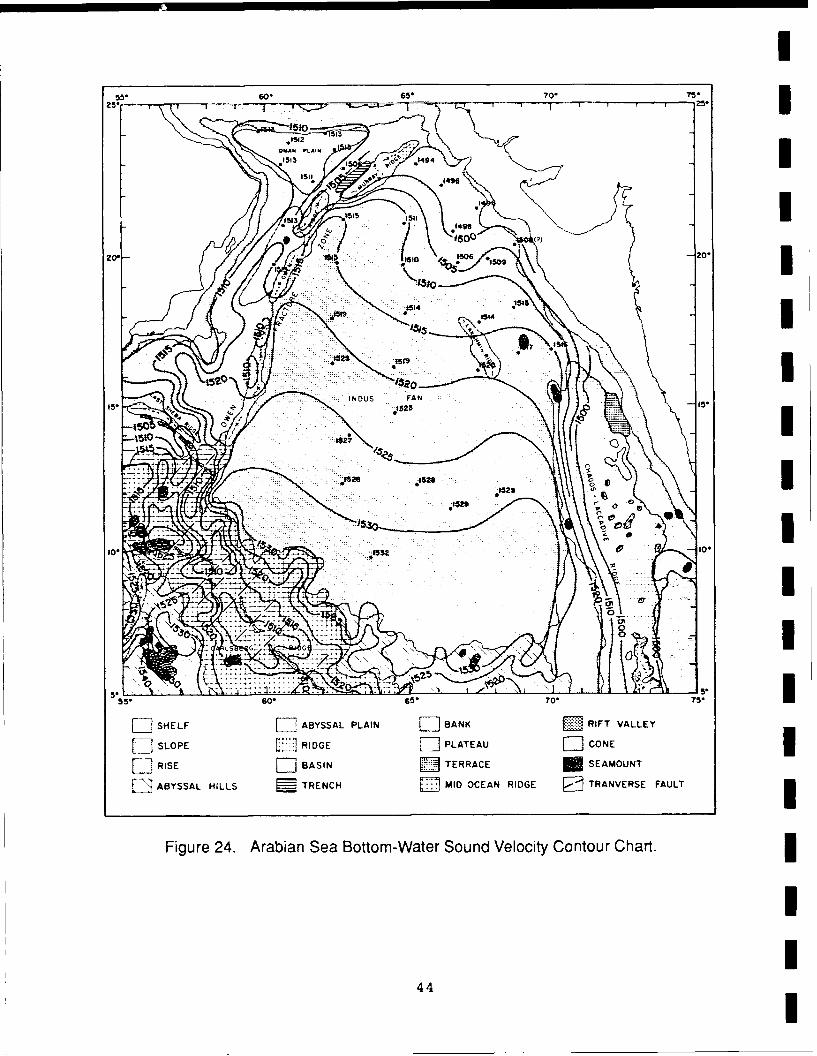
55* o. 6. 70 7525.__ 1 -7 7 25
1510 513I.1542OMAN PLAI.1513.14I
A15111513 511I
.1U20 I 20
toILI SELF BYSSL PLIN BNK RFT VLLE
SLOPERIDG PLAEAU15CON
LI RISE LI BAINDU TERAESANN
151 AYSLHLSTRNHMD3ENRDG RNES AL
Figue 2. Aabin Sa Btto-Waer oun Veociy Cntor1Cart
15ze 1115 CI
10, "O e 44
0I

55* 60, 65. 70' 7525
0.
LAI
0:97 ~ 7 0977 *' 20*
I G S 74
INDU~ FAN
I * D
10, QS70972
5,60; 70* 75
LIIISHELF F7]ABYSSAL PLAIN E]BANK E3RIFT VALLEY
MI SLOPE MRIDGE [Z PLATEAU Li CONE
D RISE BASIN TERRACE E SEAMOUNT
ElABYSSAL HILLS TRENCH MID-OCEAN RIDGE TRANVERSE FAULT
Figure 25. Sediment Surface to Bottom-Water Sound Velocity Ratio Contour Chart
of the Arabian Sea.
45
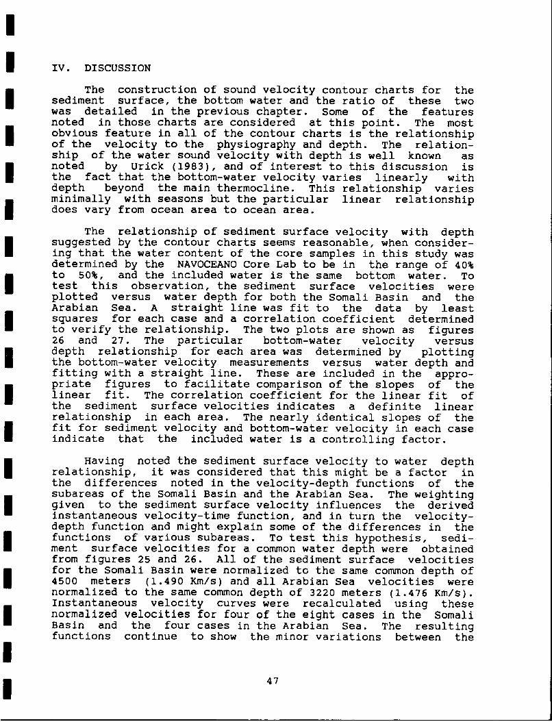
IV. DISCUSSION
The construction of sound velocity contour charts for thesediment surface, the bottom water and the ratio of these twowas detailed in the previous chapter. Some of the featuresnoted in those charts are considered at this point. The mostobvious feature in all of the contour charts is the relationshipof the velocity to the physiography and depth. The relation-ship of the water sound velocity with depth is well known asnoted by Urick (1983), and of interest to this discussion isthe fact that the bottom-water velocity varies linearly withdepth beyond the main thermocline. This relationship variesminimally with seasons but the particular linear relationshipdoes vary from ocean area to ocean area.
The relationship of sediment surface velocity with depthsuggested by the contour charts seems reasonable, when consider-ing that the water content of the core samples in this study wasdetermined by the NAVOCEANO Core Lab to be in the range of 40%to 50%, and the included water is the same bottom water. Totest this observation, the sediment surface velocities wereplotted versus water depth for both the Somali Basin and theArabian Sea. A straight line was fit to the data by leastsquares for each case and a correlation coefficient determinedto verify the relationship. The two plots are shown as figures26 and 27. The particular bottom-water velocity versusdepth relationship for each area was determined by plottingthe bottom-water velocity measurements versus water depth andfitting with a straight line. These are included in the appro-I priate figures to facilitate comparison of the slopes of thelinear fit. The correlation coefficient for the linear fit ofthe sediment surface velocities indicates a definite linearrelationship in each area. The nearly identical slopes of thefit for sediment velocity and bottom-water velocity in each caseindicate that the included water is a controlling factor.
Having noted the sediment surface velocity to water depthrelationship, it was considered that this might be a factor inthe differences noted in the velocity-depth functions of thesubareas of the Somali Basin and the Arabian Sea. The weightinggiven to the sediment surface velocity influences the derivedinstantaneous velocity-time function, and in turn the velocity-depth function and might explain some of the differences in thefunctions of various subareas. To test this hypothesis, sedi-ment surface velocities for a common water depth were obtainedfrom figures 25 and 26. All of the sediment surface velocitiesfor the Somali Basin were normalized to the same common depth of4500 meters (1.490 Km/s) and all Arabian Sea velocities werenormalized to the same common depth of 3220 meters (1.476 Km/s).Instantaneous velocity curves were recalculated using thesenormalized velocities for four of the eight cases in the SomaliBasin and the four cases in the Arabian Sea. The resultingfunctions continue to show the minor variations between the
47

I
SOMALI BASIN ISediment Surface Velocity versus Water Depth
Bottom Water Velocity versus Water Depth II
Velocity (km/sec) I1.45 1.50 1.55 1.60
1000 , , ,,-, , , ,, 4 ,,,,,
6\.S~I
2000\I
'30O00
4000 4
A I
or-
5000 >, ' II
Sediment Surface: V = 1.411 + 0.019dR = 0.771661
6000 SLDev.f 0.007869----. Bottom Water : V = 1.474 + 0.013d
R = 0.976464S.,Dev.= 0.018M86
R : Coefficient of CorrelationSliDev. = Standard Deviation
Figure 26. Sediment Surface Velocity Versus Water Depth in the Somali Basin.
I,8 I

I
I ARABIAN SEA
Sediment Surface Velocity versus Water De thBottom Water Velocity versus Water Dept
I
* Velocity (km/sec)1.45 1.50 1.55 1.60
1450 I I I ' I i , , , , , , I , , , , ,
I22450
I * " "
I o :x~3450-
I • 4450 -•I
I5450
Sediment Surface: V = 1.440 + 0.0lidR= 0.678906
SLDev.- 0.008979Bottom Water V = 1.468 + 0.015d
R-= 0.994964St.Dev.= 0.006838
R = Coefficient of CorrelationSt.Dev. = Standard Deviation
5 Figure 27. Sediment Surface Velocity Versus Water Depth in the Arabian Sea.
IIII 49

ifunctions of different areas and were not significantly differ-ent from the original functions. A comparison of two normalizedderived functions versus standard derived functions is presentedin figures 28 and 29. As was the case in the original analysis,the curves obtained did not pass through the "normalized" origin Ipoint despite the heavy weighting of this point due to thenormalization. This indicates that despite the control ofwater depth on sediment surface velocity, the velocity at depthin the sediments influences the initial velocity of the derivedfunction to a considerable extent.
In the velocity contour charts of the Somali Basin, the ihigh ratio in the southwest corner of the Basin is somewhatdisconcerting given the smooth contours of the other two charts.The sediment surface velocity chart does not indicate a high at Ithis point nor does the bottom-water contour chart indicate alow to explain the ratio high. Neither the descriptions ofDeep Sea Drilling Project (DSDP) Site 241 nor the seismiccross section of Francis et al. (1966) gives any indication ofan unusual sediment surface velocity high in this area whichwas not detected by our cores. The author concludes that it isa contouring artifact of the adjoining low just to the south- Ieast.
In the velocity contour charts of the Arabian Sea, the ratiohigh in the upper portion of the Indus Cone in figure 25 is iconsidered to be the result of the channeling effect of theLakshmi Ridge on the sediment transport, as well as the de-crease of the ratio further down the Cone. The observation wasmade earlier that the bottom-water velocity was increasing at afaster rate than the sediment surface velocity along the extentof the Cone. This is considered to be due to the transported isediments becoming finer with distance from the source at ahigher rate than the increase of bottom-water velocity withdepth. The result is a general decrease in the ratio withincreasing depth.
The fence diagram of the Somali Basin indicates a considera-ble amount of consistency in the sediment section of the Inorthern basin between Chain Ridge and the African coast. Thisis not surprising considering the limited nature of this portionof the Basin and its enclosure by coast and ridges. The south- Iern portion of the Basin shows reasonable consistency consider-ing its size. The major difference is in the very central por-tion of the southern fence diagram where slightly higher veloci-ties occur nearer the surface. Despite the variation indicatedby the fence diagrams, the individual station instantaneousvelocity functions show little variation. This is presumed tobe due to the smoothing effect of plotting curves through data mpoints in which the layer velocity is assigned to the midpointof the layer.
The fence diagrams of the Arabian Sea show quite asimilar situation. The Oman Abyssal Plain and the Owens
l50
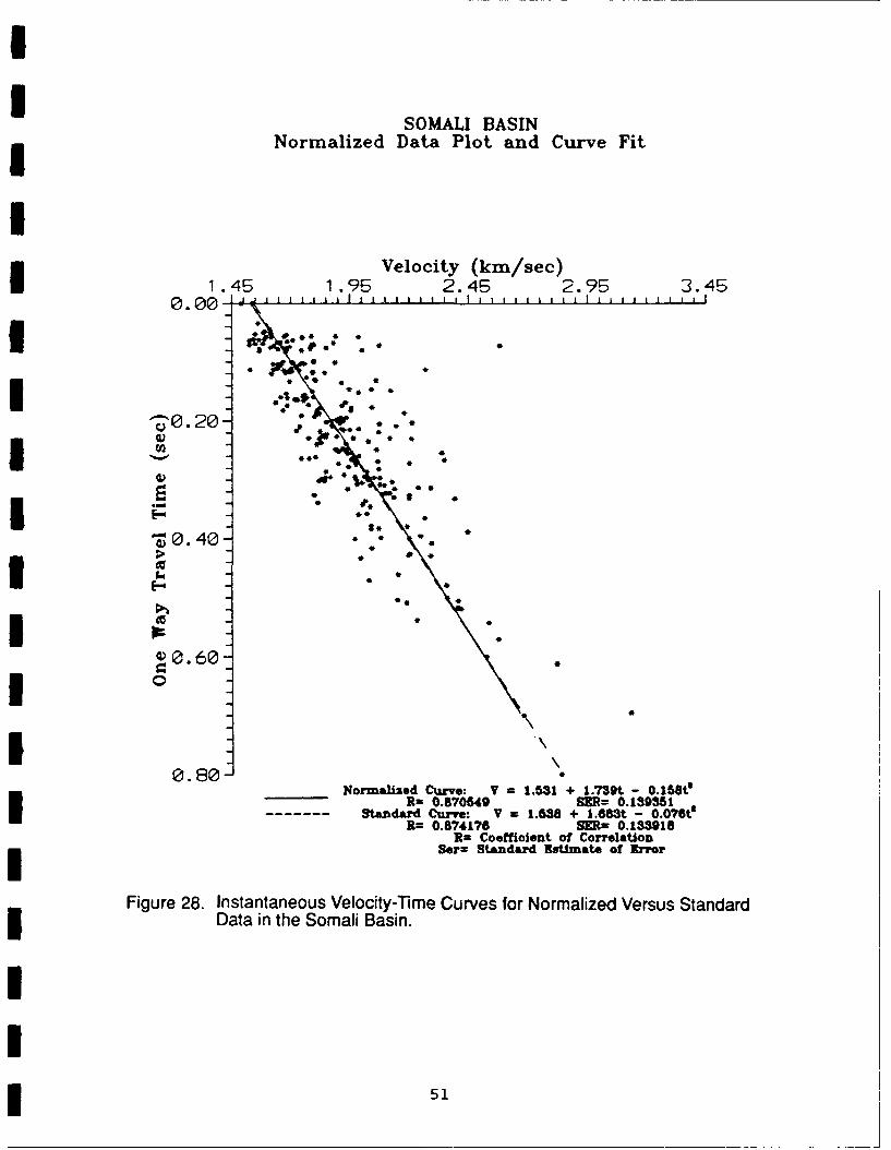
SOMALI BASINNormalized Data Plot and Curve Fit
Velocity (km/sec)1.45 1.95 2.45 2.95 3.45
0. 00- .- -
"0. 2,0..
00,.•', -...
*00.
A4
•0.60
Normalized Curve: V = 1.531 + 1.739t - 0.158t!R= 0.870849 SER= 0.139351
Standard Curve: V = 1.638 + 1.683t - 0.076eR= 0.874176 SMR= 0.133918
R= Coefficient of CorrelationSerz Standard Estlyate of Error
Figure 28. Instantaneous Velocity-Time Curves for Normalized Versus StandardData in the Somali Basin.
51

I
INDUS CONENormalized Data Plot and Curve Fit
IVelocity (km/sec) 5
1.45 2.45 3.45 4.450.00-1
.41" 44
""0 40.
E to
w 0 80
Normalized Curve: V= 1-486 + 2.8M6t - 0.772e
R= 0.971,966 SER= 0.131478120. Standard Curve: V= 1.487 + 2.874t - 0.816t!
R= 0.97,0364 SER. 0.126253R= Coefficient of CorrelaUon •
SnR= Standard Rot'ate of Error
4!
Figure 29. Instantaneous Velocity-T1ime Curves for Normalized Versus StandardData in the Arabian Sea.I
I
Abyssal Plain both show considerable consistency as did thenorthern Somali Basin, presumably for the same reason. TheIndus Cone fence diagram exhibits extensive variation through-I out. Unfortunately, all of the DSDP and Ocean Drilling Program(ODP) sites taken in the Arabian Sea have been on the fringes ofthe Indus Cone along the Chagos Laccadive Ridge or the OwensRidge. Thus, the author relies on the work of the two authorswho have conducted the bulk of the investigation of the IndusCone, B.R. Naini and V. Kolla. A basal layer following thestructural trends of the basement cited by Naini and Kolla(1981) would correspond to the >2.6 km/s layer, which seems tobe fairly uniform throughout the fence diagram. The investiga-tors believe the sediments in this basal layer were mainlyinfluenced by pelagic sedimentation while the lower velocitysediments in the upper layers were mainly deposited by turbiditesedimentation. The considerable variation in the upper layersof the fence diagram is the result of the deposition by thethree canyon complexes which migrated extensively across thefan as noted by Kolla and Coumes (1987).
The velocity ratio chart of figure 20 can be compared to aratio chart whose ratios were obtained from the tables ofHamilton (1980) shown in figure 30. Core descriptions could beused to enter table IIB, under the heading of abyssalplain and obtain the appropriate ratio. Upon attempting thiswork, it was found that all of the cores for which velocity datawere available had not yet been analyzed and description ofsediment types were not available. Of the cores taken byNAVOCEANO in the Somali Basin, only 13 had sufficient coreanalysis beyond velocity measurements for this purpose. Another16 cores with suitable analysis were found in Burroughs(1977) and 6 cores were obtained from the DSDP (Fisher et al.,1974; Simpson et al., 1974). Using the physiographic locationand the percentages of sand, silt and clay to enter the tables,a velocity ratio for each of the 35 core locations was obtainedand plotted. It is recognized that 35 data points is a limitednumber for contouring such a large area. However, this numberI of data points is sufficient to point out any obvious similari-ties or differences. It quickly became apparent that most ofthe sediments would fall into one table category (Hamilton,1980 [Table IIB, Abyssal Hill, Calcareous Pelagic Sediment]);therefore, all have the same velocity ratio. The result isshown in figure 31.
Only two points can be made with any degree of confidencebased on this comparison. First, the chart based on ratios fromthe table implies that the bulk of the area has a velocity ratiogreater than one, while the measured ratio chart shows no ratioas great as one. Secondly, there is a general agreement betweenthe two charts in that the velocity ratio in the southernportion of the basin is somewhat lower in general than that inthe northern part of the basin. The explanation for the differ-ence in the ratios obtained by NAVOCEANO and those presentea in
53

II
TABLE TIM. Abyssal plain and abyssal hill environments; sediment densities, porosities. sound 5velocities, and velocity ratios.
Density a Porosity a Velocity a
Environment (g/cM3 ) (%) (m/s) Velocity ratio a
Sediment type Av SE Av SE Av SE Av SE
Abyssal plain' 5Clayey silt 1.454 0.022 74.2 1.58 1528 3 0.999 0.002Silty clay 1.348 0.014 80.5 0.98 1515 2 0.991 0.001 3Clay 1.352 0.037 80.0 2.20 1503 2 0.983 0.001
Bering Sea and Okhotsk Sea (siliceous-diatomaceous) 3Silt 1.447 - 70.8 ... 1546 1.011 ..
Clayey silt 1.228 0.019 85.8 0.86 1534 2 1.003 0.001Silty clay 1.214 0.008 86.8 0.43 1525 2 0.997 0.001 3Abyssal hill
Deep-sea ("redi pelagic clay 3Clayey silt 1.347 0.020 81.3 0.95 1522 3 0.995 0.002Silty clay 1.344 0.011 81.2 0.60 1508 2 0.986 0.001Clay 1.414 0.012 77.7 0.64 1493 1 0.976 0.001
Calcareous pelagic sediment
Sand-sit-clay 1.435 0.007 75.3 0.38 1556 2 1.017 0.001Silt-clay 1.404 0.011 76.9 0.64 1536 1 1.004 0.001
aLaboratory values: 23 4C. 1 atm pressure; density: Saturated bulk density; porosity: Salt free; Uvelocity ratio: Velocity in sediment/velocity in sea water at 23"C. 1 atm. and salinity of sedimentpore water; SE: Standard error of the mean.
6 For approximate properties of thinner, coarser-grained layers in abyssal plain turbidities: Seecontinental terrace Tables-IA and IB in the fine sand to sand-silt-clay sizes (silt is most common).
Figure 30. Illustration of Hamilton's Table II B. I
5IIII
54 1
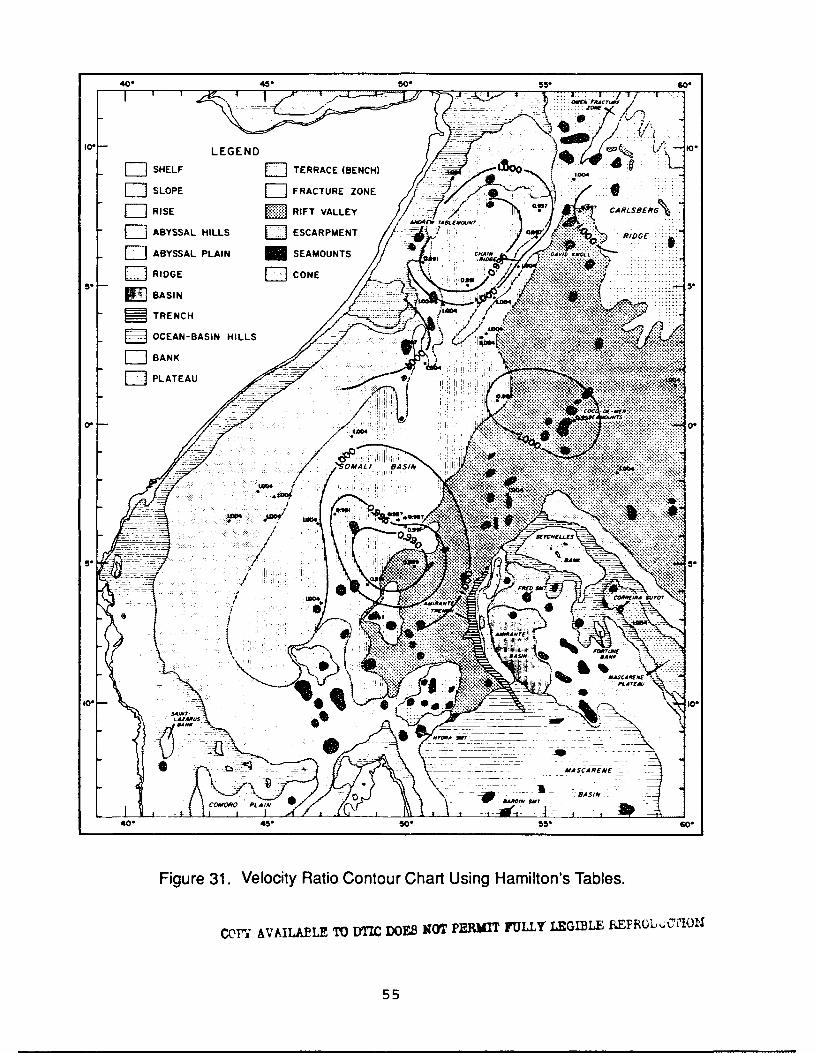
40- 45- 50. 55* 60-
10* 10.10 LEGENDSHL TERRACE (BENCH) 1%-0 too.
E1SLOPE FRACTURE ZONE 1
FIIIRISE RIFT VALLEY CRSEG
LIABYSSAL HILLS EjESCARPMENT ) ~'~RIDGE00LIABYSSAL PLAIN SEAMOUNTSX1....
SRIDGE CN
SBASIN .....
STRENCHq
010*
+ ~ ;&- - -AS \X,
55.
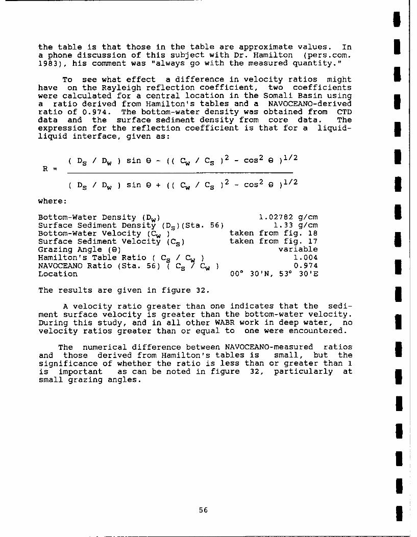
I
the table is that those in the table are approximate values. In 3a phone discussion of this subject with Dr. Hamilton (pers.com.1983), his comment was "always go with the measured quantity."
To see what effect a difference in velocity ratios mighthave on the Rayleigh reflection coefficient, two coefficientswere calculated for a central location in the Somali Basin usinga ratio derived from Hamilton's tables and a NAVOCEANO-derived Uratio of 0.974. The bottom-water density was obtained from CTDdata and the surface sediment density from core data. Theexpression for the reflection coefficient is that for a liquid-liquid interface, given as:
( Ds / Dw ) sin 9 - (( C s / Cs )2 _ cos 2 9 )1/2 3R=
( Ds / Dw ) sin e + (( C s/Cs ) 2 cos 2 )1/2 3where:
Bottom-Water Density (Dw) 1.02782 g/cm ISurface Sediment Density (Ds)(Sta. 56) 1.33 g/cmBottom-Water Velocity (Cw ) taken from fig. 18Surface Sediment Velocity (Cs) taken from fig. 17 IGrazing Angle (9) variableHamilton's Table Ratio ( Cs / Cw ) 1.004NAVOCEANO Ratio (Sta. 56) ( Cs / CW 1 0.974Location 000 30'N, 530 30'E
The results are given in figure 32. 3A velocity ratio greater than one indicates that the sedi-
ment surface velocity is greater than the bottom-water velocity.During this study, and in all other WABR work in deep water, no Ivelocity ratios greater than or equal to one were encountered.
The numerical difference between NAVOCEANO-measured ratiosand those derived from Hamilton's tables is small, but thesignificance of whether the ratio is less than or greater than 1is important as can be noted in figure 32, particularly atsmall grazing angles.
II
I
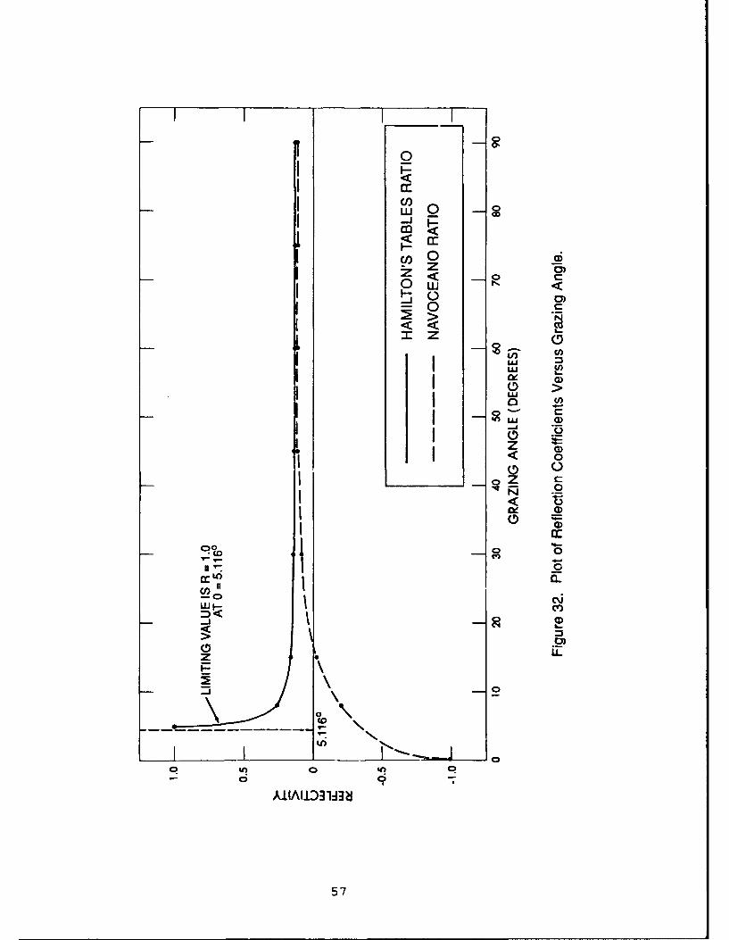
im <
<a:
<aI-
(10m z 0
-0 Cl
zzz
(DR 0>w CD
0D 0
a: oO CL
00
AIIA1103aA
00 I 50
V. CORRELATION WITH OTHER SEISMIC WORK
As mentioned earlier, considerable study of the SomaliBasin has been carried on by various investigators such asFrancis et al. (1966), Bunce et al. (1967), Davies and Francis(1964) and more recently by Coffin et al. (1986). Since Mombasawas a major port of operations during the International IndianOcean Expedition, numerous tracks were made through the Basin.Unfortunately, many of the ships participating did not haveseismic systems, and many of those with seismic systems tookonly seismic vertical reflection profiles. Aside from therefraction work by Francis et al. (1966), only a limited numberof interval velocity measurements had been made until themeasurements presented here and those recently published byCoffin et al. (1986).
The general velocity-depth structure as obtained by thisstudy and the refraction work of Francis et al. (1966) can becompared. Both studies agree that the sediment velocityincreases gradually and smoothly with depth to at least 1500meters beneath the sea floor, the limit of our penetration. Wealso agree on the velocity range of 1.50 km/sec to 1.80 km/secin the upper 1500 meters.
It is possible to correlate to the work of Coffin et al.(1986) only to a limited extent, since the bulk of our stationsin the Somali Basin were to the east of the Coffin stations.Only 11 of our stations were in the Continental Rise area in thewestern portion of the Somali Basin, whereas all but 9 to 10 oftheir stations are on the Rise. Using only those stations takenon the Rise, we derived a linear instantaneous velocity functiongiven by V = 1.544+1.569t. Their results are similar, V =1.577+1.655 t (where t is one-way travel time).
In September of 1981, we received some preliminary globalvelocity data from Houtz at Lamont-Doherty Geological Observato-ry (pers. com. 1981). These velocity functions are given in theform V= V'+ Kt where the sound velocity is expressed as afunction of one-way travel time, t, V' is the sediment surfacevelocity and K is the vertical gradient of sound. For theSomali Basin, the Lamont function is V = 1.58+1.74t. Aninstantaneous velocity function from the data of all 70 SomaliBasin stations in this study results in the function V =1.540+1.649t. Our sediment surface velocity and velocitygradient are lower than that of Houtz, but in general theagreement is good (figure 33). For example, if one predictsthe velocity of sound in the sediment at a depth equivalent toj.3 seconds of one-way travel time, a velocity of 2.102Km/sec would be obtained using the Houtz model and a velocityof 2.035 Km/sec according to the NAVOCEANO model. In the SomaliBasin, near-surface velocities derived from the DSDP are 1.47,1.48, 1.53, 1.51 and 1.58 km/sec from DSDP sites 234, 235,236, 240 and 241, respectively (Fisher et al., 1974; Simpson et
59
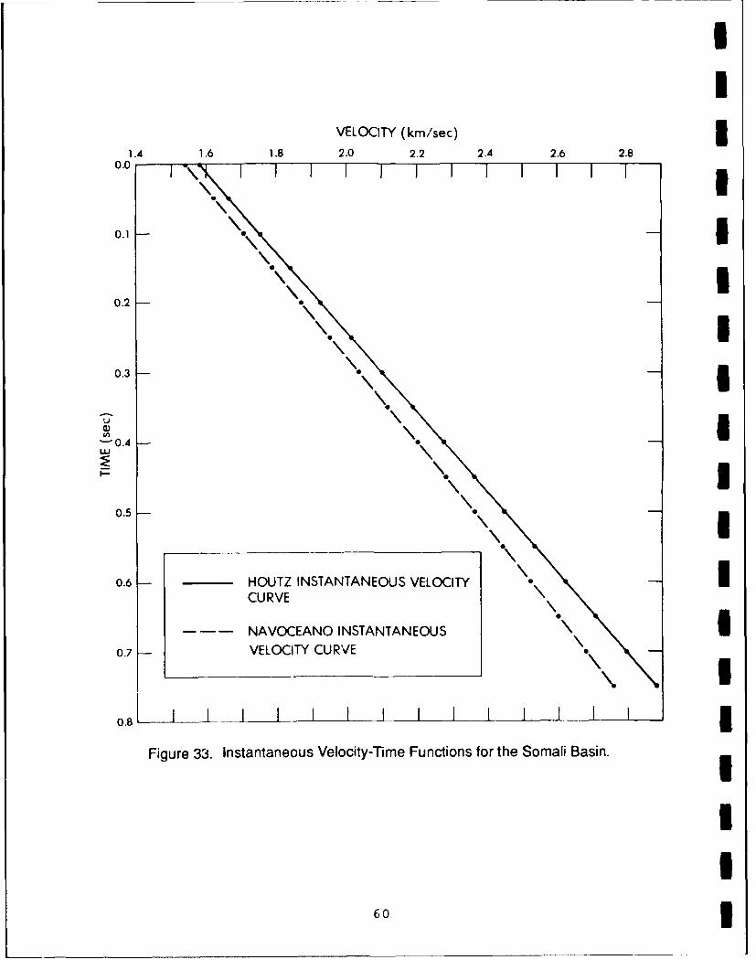
II
VELOCITY (km/sec) 31.4 1.6 1.8 2.0 2.2 2.4 2.6 2.8
0.03
0.1 3
0.2
0.3 I
'0.4
LUU0.51
0.6 -HOUTZ INSTANTANEOUS VELOCITY ICURVE
NAVOCEANOU INSTANTANEOUS I0.7 - VELOCITY CURVE I
\I
0.81 I I I I I I 3Figure 33. Instantaneous Velocity-Time Functions for the Somali Basin.
I
60 3
II al., 1974). Our sediment surface velocity of 1.540 km/sec,
obtained from our derived velocity function, falls within thisrange and is close to their mean value. The surface velocityof 1.58 km/sec reported by Houtz agrees well with the velocityfrom DSDP site 241, located on the edge of the African Conti-nental Rise, and may be more typical of a rise velocity (Simpsonet al., 1974).
I In the Arabian Sea, correlation to other data is minimaldue to the paucity of available seismic data. Considerablework was done by white and Ross (1979) in the Gulf of Oman;unfortunately, all but two of the lines were on the slope andshelf of Iran. The two lines extending into the Oman AbyssalPlain were taken with a single-channel seismic system, whilemost of the other lines were taken with a multichannel system.The two abyssal plain lines run essentially north-south, andindicate a thick sediment sequence at the northern end, gradual-ly thinning toward the southern end. Our lines were east-west,but each successive line progressed to the south and theyindicate a thinning sequence as well. In the Owens AbyssalI Plain, only the DSDP site 223 could be reasonably considered forcorrelation. Other DSDP sites were located on the Owen Ridgeand ODP sites were also located on the Ridge or on the ArabianContinental Slope or Rise. Site 223 was located just west ofI the Ridge on its slope, but velocities should be comparable.The velocities obtained by DSDP varied little from 1.55 km/secin the upper 240 meters and from 1.60 to 1.75 km/sec in the next220 meters (Whitmarsh et al., 1974). Below this, velocitiesincrease to 1.8 to 2.0 km/sec and our results are in agreementwith these.
In 1977, prior to the start of this study, a series of eightWABR stations was taken by NAVOCEANO on the Indus Cone. Six ofthese stations ran in a north-south direction on the Cone andI were analyzed and reported by Bachman and Hamilton (1980).Their 5eported velocity-depth function is V = 1.510+1.200D-0.253D +0.034D . In this study, we characterized the IndusCone by two velocity-depth functions, one for the upperportion of the Cone (within 160 miles of shore) and one for theremainder of the Cone. The function derived for the main por-tion of the Cone is V = 1.488 + 1.754D - 0.622D2 and is repre-sentative of the area from which Bachman's function was derived.A plot of each is shown for comparison in figure 34. The twofunctions differ considerably in gradient, with theirsI indicating a higher gradient at depth. Our function is derivedfrom the data of all but three of the stations taken on the Conearid therefore is an averaging of the functions throughout the
m Cone.
The instantaneous velocity function obtained by Naini andTalwani (1977) V = 1.534+1.965t is compared to the instantaneousI velocity function obtained for the middle Cone area in thisstudy (V = 1.549+2.221t), and the instantaneous velocity func-tion derived by Bachman and Hamilton ( V = 1.510+1.863t,
mm 61

III
VELOCITY IN KM/SEC
1.4 1.6 1.8 2.0 2.2 2.4 2.6 2.8 3.0 3.2 30
0.2 10.4
S0.6
0.8
I'-
LU 1.0 11.2
1.4 11.6 3
BACHMAN AND HAMILTON (1980)
V = 1.510 + 1.200h - 0.253h 2 + 0.034h 3
NAVOCEANO
V = 1.488 + 1.754h - 0.622h2
Figure 34. Velocity-Depth Functions for the Indus Cone.
6IIII
1980) is included in this plot for comparison (figure 35).Again, it is noted that our function is a synthesis of data fromnumerous stations and thus reflects the effects of considerablevariation in sediment sections throughout the Cone, while theother two functions reflect only a limited portion.
DSDP site 221 lies at the southeastern edge of the Cone andthe uppermost velocity obtained from their coring was 1.41km/sec, somewhat lower than the values we obtained in that area(Whitmarsh et al., 1974). The remainder of their cores hadvelocities from 1.45 to 1.74 km/sec and our values are in gener-al agreement with these.
63
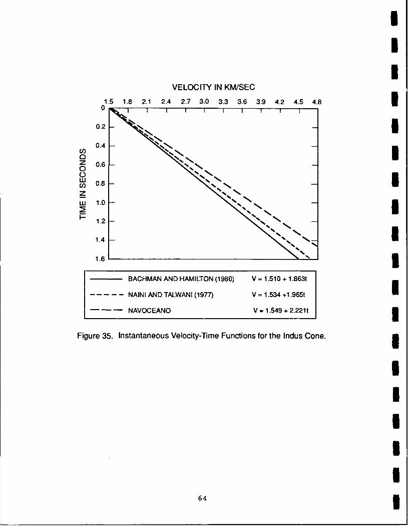
III
VELOCITY IN KM/SEC
1.5 1. 8 2. 1 2. 4 2 .7 3.0 3.3 3.6 3.9 4. 2 4. 5 4.8I
0.2 I0.4
0 ,.. -% .--. _0 Z .6 I
BAC0AN NDHMLO(18) V=150+.8t
(n 0.8
1.4 N, N
1.613
BACHMAN AND HAMILTON (1980) V = 1.510 + 1.863t
NAINI AND TALWANI (1977) V = 1.534 +1.965t INAVOCEANO V =1.549 +2.221 t
Figure 35. Instantaneous Velocity-Time Functions for the Indus Cone.
IIIII
64 1
VI. SENSITIVITY ANALYSIS
There is an inherent factor in WABR affecting the sensi-tivity of all measurements. That factor is the drift of thesonobuoy after it has been deployed. There are some extremelystrong currents in the Somali Basin about 5 to 50 milesoffshore. These currents can be most disrupting, as was pointedout by Coffin et al. (1986) where a considerable amount of theirwork was in that area. On the inshore portions of some of ourcruise legs in this area we experienced currents on the order of12 to 15 knots. Fortunately, none of our WABR measurements weretaken in this area but were taken some 300 miles or more out tosea where the drift of the sonobuoys was almost negligible overthe period of the measurement. The same was true of the meas-urements made in the Arabian Sea.
As noted earlier, the WABR method is based on the Dixmethod developed for land reflection seismic exploration. Inland exploration, the distance between source and receiver issmall compared to the distances encountered in marine work, andray parameters, or apparent velocity, are zero. Generally, inland work, the distance between the source and the furthestreceiver is only a few thousand feet, whereas at sea this dis-tance approaches 10 nautical miles. In the Dix method, therefraction or bending of rays between source and reflector isnot considered, and simple straight line geometry is assumed forthe reflections when plotted X2 -T 2 . In land work the refractioneffect is minimal, except where very strong velocity gradientsare detected. In marine WABR work, this refraction effectshows up as a slight amount of curvature in the distal end ofthe X2 -T 2 plot giving rise to some problems in curve fitting.In this study, the limitations of the source level allowed apenetration of the sediments only on the order of 1200 to 1500meters and the generally small gradual increase in velocity withdepth caused little refraction at interfaces, and the assumptionof straight line geometry is reasonable. This assumption isreflected in the lack o5__o the minimal amount of curvature inthe distal ends of the X T plots.
Other investigators have developed a rule of thumb in thatintervals between horizons chosen for study should not be lessthan 1/12 the depth of the water column. In general, this ruleof thumb was followed in this study except in cases of unusuallygood reflecting horizons giving rise to intervals slightly lessthan 1/12 the water depth in thickness. Jim Matthews of theNaval Research Laboritory (NRL) studied the sensitivity of thefactors involved in the wide-angle reflection method andconcluded that the method was not particularly sensitive to theinterval thickness as long as noise is not a major factor (pers.com. 1990).
A major point of sensitivity in the overall method arisesin conversion of the interval velocity versus one-way traveltime from the sediment surface to an instantaneous velocity-time
65

Ufunction. In water depths of 4000 to 5000 meters, using therule of thumt, the first interval thickness is from 300 to 400meters. When plotting the interval velocity at the midpoint ofthe interval, this point is from 150 to 200 meters from thesediment surface. After all of the interval velocities have ibeen plotted at the midpoints of the intervals, a curve is fit
to the data points. The point of sensitivity arises from thefact that without a data point at the sediment surface, there isno curve origin point to control the least squares fit, thusplacing no limits on the initial velocity gradient. It isimportant, as pointed out by Hamilton (1974), to obtain a sedi-ment surface velocity and force the curve through this point.
The methods used in this study to acquire and process thedata have been used by investigators such as Houtz et al. (1968)and Bachman and Hamilton (1980) for some time and are sensitiveprimarily to attention to detail in the method of acquisitionand to the detail and accuracy in reading travel times. Routinecalibration of the acquisition components is necessary for thevalidity of the travel time data. The sensitivity of the analy-sis is predominantly in the comparison of instantaneous velocityfunctions and the detection of whether anomalous instantaneous Ivelocity functions are true anomalies or reflecting problems inthe acquisition and processing of that particular station. Acheck of the raw data and reflection profile will generallydetermine if there was a problem in the acquisition or process-ing of the data. If this is not the case, then othermeasurements must be taken in the same location to verify thatthe measurement was truly anomalous. A simultaneous verticalreflection profile during the WABR run is most helpful in assur-ing that the critical assumption of flat bottom and parallellayers is met.
IIIIiI
66

VII. CONCLUSIONS
The primary conclusion of this study is that a velocity-depth function representative of the sediment velocity-depthrelationship throughout a large ocean area can be derived froman adequate velocity-depth sampling in that area. The derivedfunction will not describe the precise velocity-depth relation-ship in the sediments of any specific site, but is a reasonablerepresentative of that relationship. In this study, thederived function describes the velocity-depth relationship inthe upper 1200 to 1500 meters of the sediment section with apossible calculated error of 210 m/sec.
For the areas considered in this study, these functionsI are : A. SOMALI BASINV= 1.539 + 1.010d - 0.166d 2
B. ARABIAN SEA1. Oman Abyssal Plain
V= 1.513 + 1.696d - 0.649d 2
2. Owens Abyssal PlainV= 1.483 + 1.465d - 0.401d 2
3. Upper Indus ConeV= 1.460 + 1.581d - 0.907d 2
4. Lower Indus ConeV= 1.488 + 1.754d - 0.622d2
The area in which each of the above Arabian Sea functionsapplies is indicated in figure 36. These functions describe thevelocity profiles of the upper 1200 to 1500 meters of thesediment section in the individual areas. In the Somali Basin,Oman Abyssal Plain and Owens Abyssal Plain, the velocity-depthfunctions describe a condition of terrigenous sedimentation andan upper sediment section consisting largely of turbidite flows.The Indus Cone velocity-depth functions describe a condition ofvoluminous terrigenous deposition primarily from one source witha mechanical segregation of material progressing away from thesource and turbidite flows overall.
In other areas of the world's oceans of similar depo-sitional environment where little or no data are available, theresults obtained in this study may be used to derive generalizedfunctions. Sediment surface velocity from core data can beused as the initial data point for a linear instantaneousvelocity function of the Houtz type. The gradient for thisfunction could be obtained from one of the functions derived foran area of similar depositional environment described in thisstudy. The function so obtained could then be developed into avelocity-depth function in the manner described earlier.
A second conclusion reached in this study is that thesediment surface velocity of deep water sediments is linearlyrelated to water depth. This appears to be due to the includedbottom water of the surface sediments. This conclusion was
67
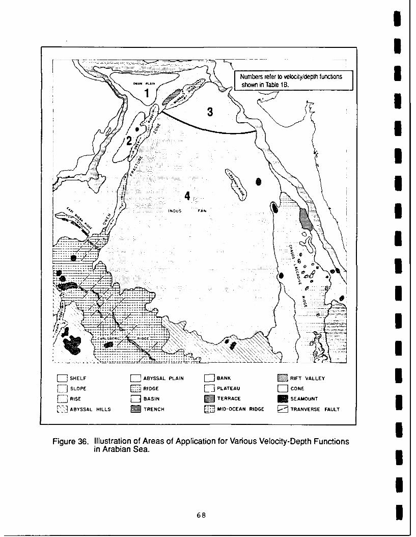
Numbers refer to velocity/depth functions iOMAN LAINshown in Table 1lB.€ '
... ...... V, 01,:':::
&I I
ARLSEfG_ RIG=
W SHELF [] ABYSSAL PLAIN BANK RIFT VALLEY 3D] SLOPE E RIDGE L]PLATEAU S CONE
F] RISE D BASIN W TERRACE W SEAMOUNT
ABYSSAL HILLS F TRENCH F MID-OCEAN RIDGE [] TRANVERSE FAULT
Figure 36. Illustration of Areas of Application for Various Velocity-Depth Functionsin Arabian Sea. i
68i

reached in the course of an effort to chart the sediment surfacesound velocity to bottom water sound velocity ratio for theareas under investigation. As a consequence of this effort, theauthor also reached the conclusion that this velocity ratio, indeep water, is generally less than 1.0. All of the velocityratios determined in this study and in all subsequent work bythe author have supported this conclusion. This conclusion isin line with the observation of Fry and Raitt (1961) that sedi-ment surface velocities are generally 2% lower than the bottom-water velocities in the Pacific Ocean.
69
VIII. RECOMMENDATIONS FOR FUTURE WORK
Considering the primary conclusion reached in this study,it would only be consistent to recommend that other suitablelarge ocean areas be characterized in the same manner as the twoareas in this study. In fact, work is underway to do just thatin large areas of the South Atlantic Ocean.
One deficiency in the WABR method was cited earlier. Thefirst data point, other than a surface sediment measurement froma core, occurs at depths of 150 to 200 meters or more becauseour source and receiver are far away from the boundary of inter-est. Those interested in modeling higher frequencies areinterested in greater detail in the upper few hundred meters,which cannot be obtained using this method. If such detail isneeded, it is recommended that a similar sampling arrangement tothe one in this study be carried out with a system such as the"Deep Towed Array Geophysical System" (DTAGS). This system,developed by NRL, consists of a deep towed source and multi-channel array. It collects multichannel data in the upper fewhundred meters and has definition on the order of meters. Thesedata could define the velocity structure of the upper fewhundred meters in detail and could be used to adjust or modifythe upper portion of the velocity-depth curve obtained byWABR methods.
The processing method used in this study for obtaininginterval velocities and thicknesses is very labor intensive. Atthis time, WABR records are read by hand and the travel timesrecorded on tabulation sheets before being entered into theinterval velocity computer program. The work is tedious andrequires approximately 3 to 4 hours per record from initialsetup to tabulation sheet by an experienced person. During thisprocess, there are numerous opportunities for the introductionof errors such as those in the reading of travel times or thoseproduced by the transposition of digits during the recording ofthe travel times.
I recommend that this process be modernized by acquiringthe data digitally and processing it digitally for velocitiesand thicknesses, as is commonly done in the oil industry.Presently, work is underway at NAVOCEANO to accomplish this. Adigital acquisition system was purchased and has been taken tosea to acquire data. The data are recorded on nine-track tapewith three tapes being required for each WABR run. During acruise in which 15 to 20 WABR runs are made, a considerableamount of tape is expended and results in additional storage andshipping problems. To alleviate this problem, a disc storagesystem for the recording of the data will be installed in thenear future. It is planned to use a technique employing avelocity analysis module to compute the trace to trace coher-ence of events as a function of normal incidence travel timeand obtain stacking velocities to derive interval velocities andthicknesses.
71
IX. REFERENCES
Bachman, R.T., and E.L. Hamilton; Sediment sound velocitiesfrom sonobuoys; Arabian Fan, J. Geophys. Res., 85,849-852, 1980.
Bunce, E.T., M.G. Langseth, et al.; Structure of the westernSomali Basin, J. Geophys. Res., 72, 2547-2555, 1967.
Burroughs III, R.H.; Structural and sedimentological evolu-tion of the Somali Basin; Paleooceanographic interpreta-tions, WHOI-77-34, 1977, Woods Hole OceanographicInstitution, Woods Hole, MA.
Clay, C.S., and P.A. Rona; Studies of seismic reflectionsfrom thin layers on the ocean bottom in the Western NorthAtlantic, J. Geophys. Res., 70, 855-869, 1965.
Cochran, J.R.; The Somali Basin, Chain Ridge and the originof the northern Somali Basin gravity and geoid low,J. Geophys. Res., 93, N. B10, 11985-12008, 1988.
Coffin, M.F., P.D. Rabinowitz, and R.E. Houtz; Crustalstructure in the Western Somali Basin, Geophys. J. R.Astr. Soc., 86, 331-369, 1986.
Davies, D., and T.J.G. Francis; The crustal structure of theSeychelles Bank, Deep Sea Research, Vol. II, 921-927,1964.
Dix, H.C.; Seismic velocities from surface measurements,Geophysics, 20, 68-86, 1955.
DuToit, A.L.; Our wandering continents, Edinburgh, Scotland,Oliver and Boyd, 1937.
Ewing, M., S. Eittreim, et al.; Sediment distribution in theIndian Ocean, Deep Sea Research, Vol. 16, 231-248, 1969.
Fisher, R.L., E.T. Bunce, et al.; Initial Reports of theDeep Sea Drilling Projects, Vol. 24, 249-389, U.S.Government Printing Office, Washington, DC, 1974.
Francis, T.J.G., D. Davies, and M.N. Hill; Crustal structurebetween Kenya and the Seychelles, Phil. Trans. Roy.Soc., London, A, 259, 240-261, 1966.
Fry, J.C., and R.W. Raitt; Sound Velocities at the Surfaceof Deep Sea Sediments, J. Geophys. Res., 66, 589-597,1961.
Hamilton, E.L.; Telephone conversation with author, August1983.
73
I
Hamilton, E.L.; Geoacoustic modeling of the seafloor, UJ. Acoust. Soc. Am., 68(5), 1313-1340, 1980.
Hamilton, E.L., D.G. Moore, et al.; Sediment velocities fromsonobuoys: Bay of Bengal, Bering Sea, Japan Sea, and NorthPacific, J. Geophys. Res., 79, 2653-2667, 1974.
Houtz, R.; Letter to Allan Lowrie at NAVOCEANO, September i1981.
Houtz, R., J. Ewing, and X. LePichon; Velocity of deep sea isediments from sonobuoy data, J. Geophys. Res., 73, 2615-2641, 1968.
Houtz, R., J. Ewing, and P. Buhl; Seismic data from sonobuoystations in Northern and Equatorial Pacific, J. Geophys.Res., 75, 5093-5111, 1970. 3
Kolla, V., P.K. Ray, and J.A. Kostecki; Surficial Sedimentsof the Arabian Sea, Marine Geology, 41, 183-204, 1981.
Kolla, V. and F. Coumes; Morphology, internal structure,seismic stratigraphy and sedimentation of Indus Fan,Am. Assoc. Petr. Geol., 71, 650-677, 1987.
LePichon, X., J. Ewing, and R. Houtz; Deep-sea sedimentvelocity determination made while reflection profiling,J. Geophys. Res., 73, 2597-2614, 1968.
Matthews, James E.; Conversation with author, April 1990.
Menard, H.W., and T.E. Chase; Fracture zones, in THE SEA,Vol. IV, Part 1, ed. A. E. Maxwell, 421-444, New York, NY,Wiley Interscience, 1970. 3
Naini, B.R. and V. Kolla; Acoustic character and thicknessof sediments of the Indus Fan and the continental marginof Western India, Mar. Geol., 47, 181-195, 1981.
Naini, B.R. and M. Talwani; Sediment distribution and struc-tures in the Indus Cone and western continental marginof India (Arabian Sea), E.O.S., Trans. Am. Geophys.Union, 58, p. 405 (abstract), 1977.
Simpson, E.S.W., Schlick, R., et al.; Initial Reports of the IDeep Sea Drilling Project, Vol. 25, 65-138, U.S.Government Printing Office, Washington, DC, 1974.
Urick, R.J.; Principles of Underwater Sound, 3rd edition,New York, NY, McGraw-Hill, Inc., 1983.
i

White, R.S., and K. Klitgord; Sediment deformation andplate tectonics in the Gulf of Oman, Earth and PlanetaryScience Letters, Vol. 32, 199-209, 1976.
White, R.S., and D.A. Ross; Tectonics of the western Gulfof Oman, J. Geophys. Res., 64, 3479-3489, 1979.
Whitmarsh, R.B., C.E. Weser, D.A. Ross, et al.; InitialReports of the Deep Sea Drilling Project, Vol. 23,U.S. Government Printing Office, Washington, DC, 1974.
Windsor, Sara; Conversations with author, Summer 1982.
75

IIi
IIIII
IIIIIIII,I
* A-1
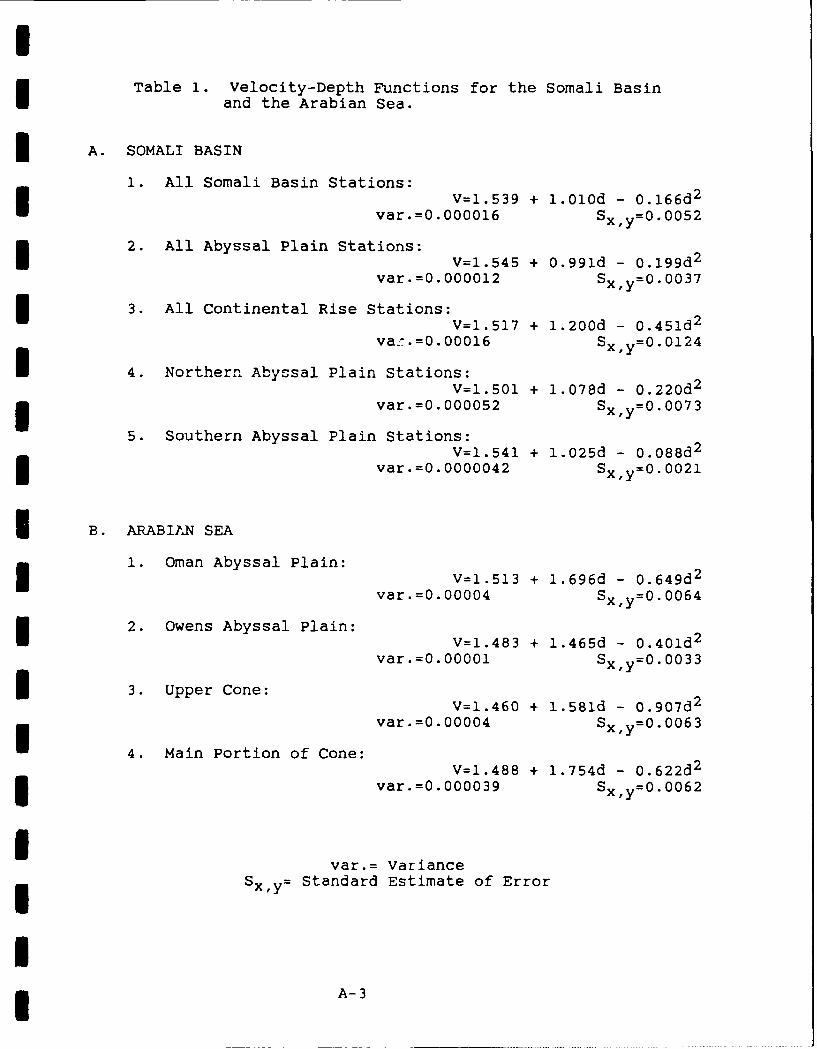
ITable 1. Velocity-Depth Functions for the Somali BasinI and the Arabian Sea.
* A. SOMALI BASIN
1. All Somali Basin Stations:V=1.539 + 1.010d - 0.166d 2
var.=0.000016 Sx~y=0.0052
2. All Abyssal Plain Stations:i V=1.545 + 0.991d - 0.199d 2
var.=0.000012 Sxfy=0.0037
3. All Continental Rise Stations:-- V=1.517 + 1.200d - Q.451d 2
va:.=0.00016 Sx,~y=0.0124
S4. Northern Abyssal Plain Stations:V=1.501 + 1.078d - 0.220d2
var.=0.000052 Sx-y=0.0073
5. Southern Abyssal Plain Stations:V=1.541 + 1.025d - 0.088d 23 var.=o.0000042 Sx y=O.O021
S B. ARABIAN SEA1i. Oman Abyssal Plain:
1V=1.513 + 1.696d - 0.649d 2
var.=o.00004 SX,y=O=. 0 0 6 4
S2. Owens Abyssal Plain:2.OesAyslPan V=1.483 + 1.465d - 0.401d2
var.=0.00001 Sx,y=0. 0 0 3 3I 3. Upper Cone:V=1.460 + 1.581d - 0.907d 2
Svar.=0.00004 Sx~y=0.0063
4. Main Portion of Cone:
V=1.488 + 1.754d - 0.622d 2
var.=0.000039 SxJy=0.0062
- var.= VarianceSxy= Standard Estimate of Error
-- A-3
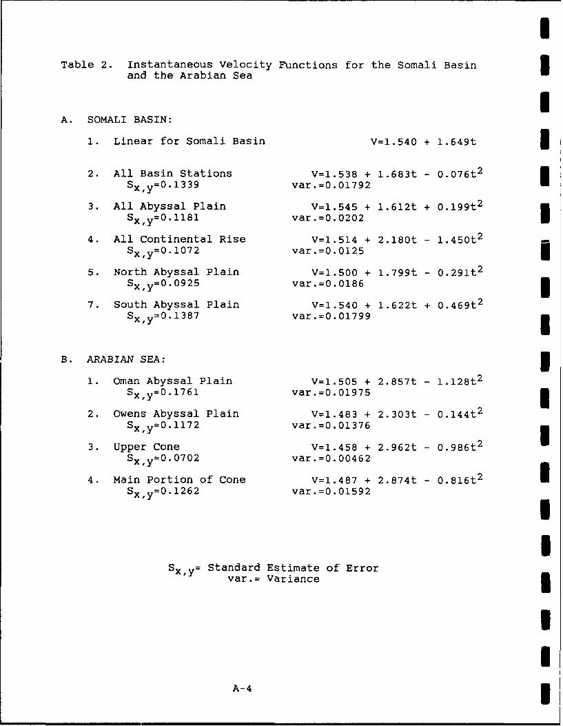
iTable 2. Instantaneous Velocity Functions for the Somali Basin
and the Arabian Sea
IA. SOMALI BASIN:
1. Linear for Somali Basin V=1.540 + 1.649t 32. All Basin Stations V=1.538 + 1.683t - 0.076t 2
Sx.y =0.1339 var.=0.01792
3. All Abyssal Plain V=1.545 + 1.612t + 0.199t 2
Sx,y =0.1181 var.=0.0202
4. All Continental Rise V=1.514 + 2.180t - 1.450t 2
Sxy=0.1072 var.=0.0125 j5. North Abyssal Plain V=1.500 + 1.799t - 0.291t 2
Sx~y=0.0925 var.=0.0186 37. South Abyssal Plain V=1.540 + 1.622t + 0.469t 2
Sx~y=0.1387 var.=0.01799 i
B. ARABIAN SEA: 31. Oman Abyssal Plain V=1.505 + 2.857t - 1.128t 2
SxIy=0.1761 var.=0.01975 i
2. Owens Abyssal Plain V=1.483 + 2.303t - 0.144t 2
Sx~y =0.1172 var.=0.01376
3. Upper Cone V=1.458 + 2.962t - 0.986t 2
Sx~y =0.0702 var.=0.00462
4. Main Portion of Cone V=1.487 + 2.874t - 0.816t 2 ISx0y =0.1262 var.=0.01592
ISx,y= Standard Estimate of Error
var.= Variance
i
A-4 3

ITable 3. Tabulation of Interval Velocities and Layer
Thicknesses in the Somali Basin
LAYER WATERSTATION LAYER VELOCITY THICKNESS DEPTH LOCATION
LAT. LONG.
(m/sec) (M) (M)
53 1492 000 4543 01°351S 54°42'EA 1562 105B 2269 210
A&B 2001 320
54 1501 000 4778 00'30'S 53C59 1 EA 1851 282
55 1506 000 4938 00°21'N 53°31'EA 1792 249
56 1510 000 5072 01'51'N 52'26'EA 1750 206B 1988 566
A&B 1921 773
57 1511 000 5079 02'17'N 51'59 1 EA 1582 219B 2212 291
A&B 1915 517
58 1499 000 4858 03'44'N 50'40'EA 1894 858B 2152 219
A&B 1944 1079
59 1495 000 4953 05'08'N 51'08'EA 1616 189B 2043 244C 2075 299
A&B 1844 436B&C 2061 543
60 1502 000 5015 04°44'N 51°27'EA 1542 189B 1969 556
A&B 1850 749
61 1512 000 5089 04'17'N 51'53'EA 1527 344B 1867 261
A&B 1666 608
A-5
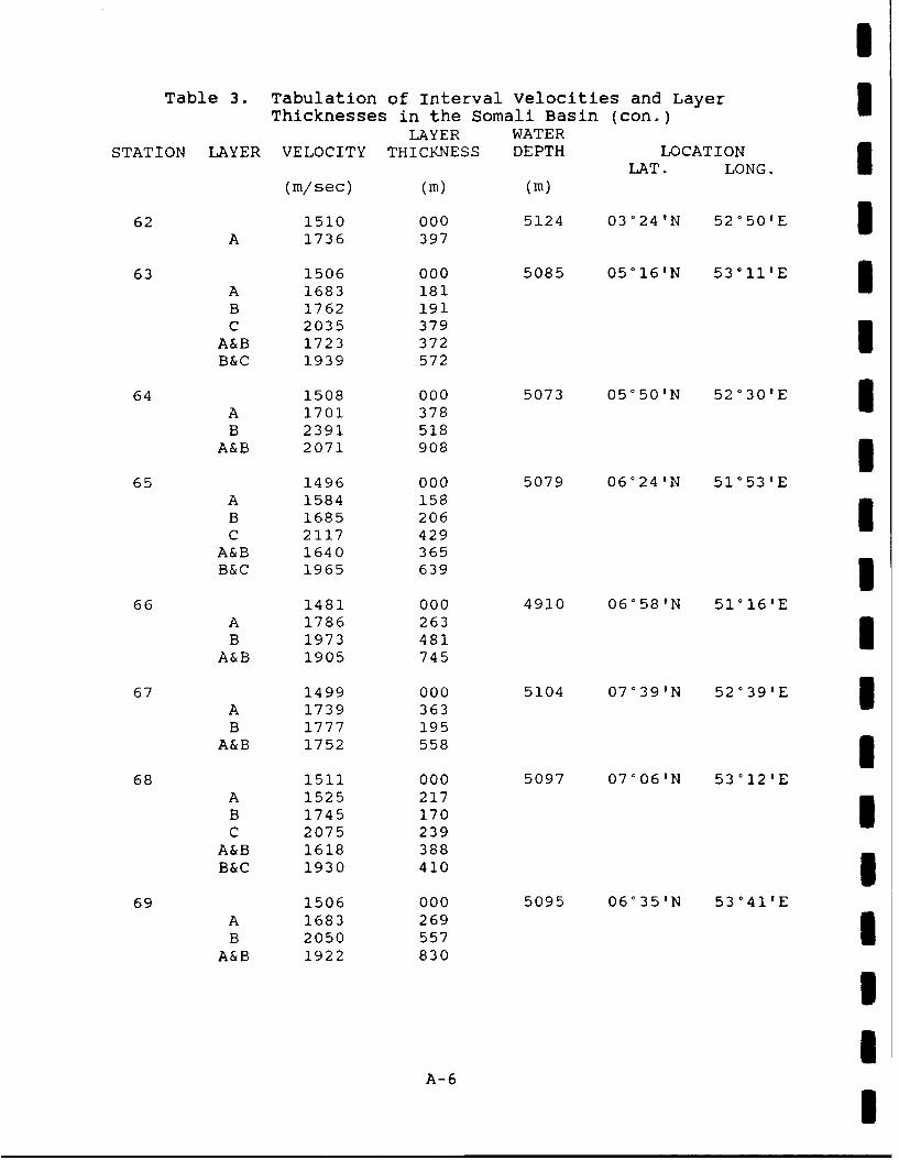
iTable 3. Tabulation of Interval Velocities and Layer
Thicknesses in the Somali Basin (con.)LAYER WATER
STATION LAYER VELOCITY THICKNESS DEPTH LOCATIONLAT. LONG.
(m/sec) (M) (M)
62 1510 000 5124 03'24'N 52'50'EA 1736 397
63 1506 000 5085 05'16'N 5311'EA 1683 181B 1762 191C 2035 379
A&B 1723 372 IB&C 1-939 572
64 1508 000 5073 05'50'N 52'30'EA 1701 378B 2391 518
A&B 2071 908
65 1496 000 5079 06'24'N 51°53'EA 1584 158B 1685 206C 2117 429
A&B 1640 365B&C 1965 639 3
66 1481 000 4910 06'58'N 51 0 16'EA 1786 263B 1973 481
A&B 1905 745
67 1499 000 5104 07'39'N 52'39'EA 1739 363B 1777 195
A&B 1752 558
68 1511 000 5097 07'06'N 53 0 12'EA 1525 217B 1745 170C 2075 239
A&B 1618 388B&C 1930 410
69 1506 000 5095 06'35'N 53°41'EA 1683 269B 2050 557
A&B 1922 830
II
A- 6 I
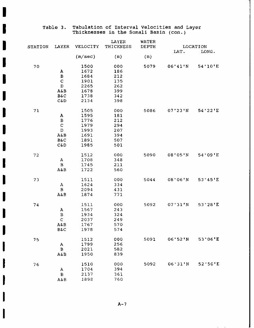
Table 3. Tabulation of Interval velocities and LayerThicknesses in the Somali Basin (con.)
LAYER WATERSTATION LAYER VELOCITY THICKNESS DEPTH LOCATION
LAT. LONG.(m/sec) (M) (M)
70 1500 000 5079 06°41'N 54°10'EA 1672 186B 1684 212C 1901 135D 2265 262
A&B 1678 399B&C 1738 342C&D 2134 398
71 1505 000 5086 07°23'N 54°22'EA 1595 181B 1776 212C 1979 294D 1993 207
A&B 1691 394
B&C 1891 507C&D 1985 501
72 1512 000 5090 08°05'N 54°09'EA 1708 348B 1745 211
A&B 1722 560
i 73 1511 000 5044 08'06'N 53*45'EA 1624 334B 2094 431
I A&B 1874 771
74 1511 000 5092 07°31'N 53°28'EA 1567 243B 1934 324C 2037 249
A&B 1767 570B&C 1978 574
75 1512 000 5091 06°52'N 53'06'EA 1799 256B 2021 582
A&B 1950 839
76 1510 000 5092 06'31'N 52°50'EA 1704 394B 2137 361
A&B 1898 760
IA-7
I

I
Table, 3. Tabulation of Interval Velocities and Layer UThicknesses in the Somali Basin (con.)
LAYER WATER 3STATION LAYER VELOCITY THICKNESS DEPTH LOCATION
LAT. LONG.(m/sec) (M) (M)
77 1509 000 5091 06'09'N 52°37'EA 1550 160B 1717 206C 2085 424
A&B 1642 366B&C 1956 633
78 1508 000 5095 05'56'N 52°31'EA 1627 366B 2200 445
A&B 1915 819
79 1500 000 5088 05'22'N 52°04'EA 1659 347B 2127 399
A&B 1892 750
80 1505 000 5091 04'57'N 51'55'EA 1759 364B 1846 329
A&B 1800 693
81 1508 000 5077 04o36,N 51'491E iA 1565 193B 1753 149C 1971 340
A&B 1644 343B&C 1902 490
82 1512 000 5094 04'12 1 N 51'43'EA 1795 354B 1849 328
A&B 1821 683
83 1515 000 5107 03'44'N 51'30'EA 1643 220B 1932 133C 2347 296
A&B 1747 355B&C 2209 431
I
A-8
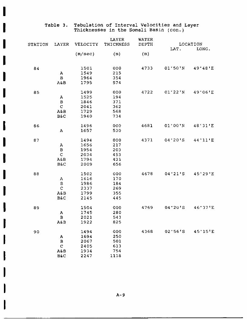
Table 3. Tabulation of Interval velocities and LayerThicknesses in the Somali Basin (con.)
LAYER WATERSTATION LAYER VELOCITY THICKNESS DEPTH LOCATION
LAT. LONG.(m/sec) (M) (M)
84 1501 000 4733 01 0 50'N 49'48'EA 1549 215B 1964 354
A&B 1795 574
85 1499 000 4722 01°22'N 49'06'EA 1525 194B 1846 371C 2041 362
A&B 1729 568B&C 1940 734
86 1496 000 4681 01°00'N 48'31'EA 1657 530
87 1494 000 4371 04°20'S 44°11'EA 1656 217B 1954 203C 2034 453
A&B 1794 421B&C 2009 656
88 1502 000 4678 04°21'S 45'29'EA 1616 170B 1986 184C 2337 269
A&B 1799 355B&C 2145 445
89 1504 000 4769 04°20'S 46°37'EA 1745 280B 2021 543
A&B 1922 825
90 1494 000 4368 02'56'S 45°15'EA 1694 250B 2067 501C 2405 613
A&B 1934 754B&C 2247 1118
A-9
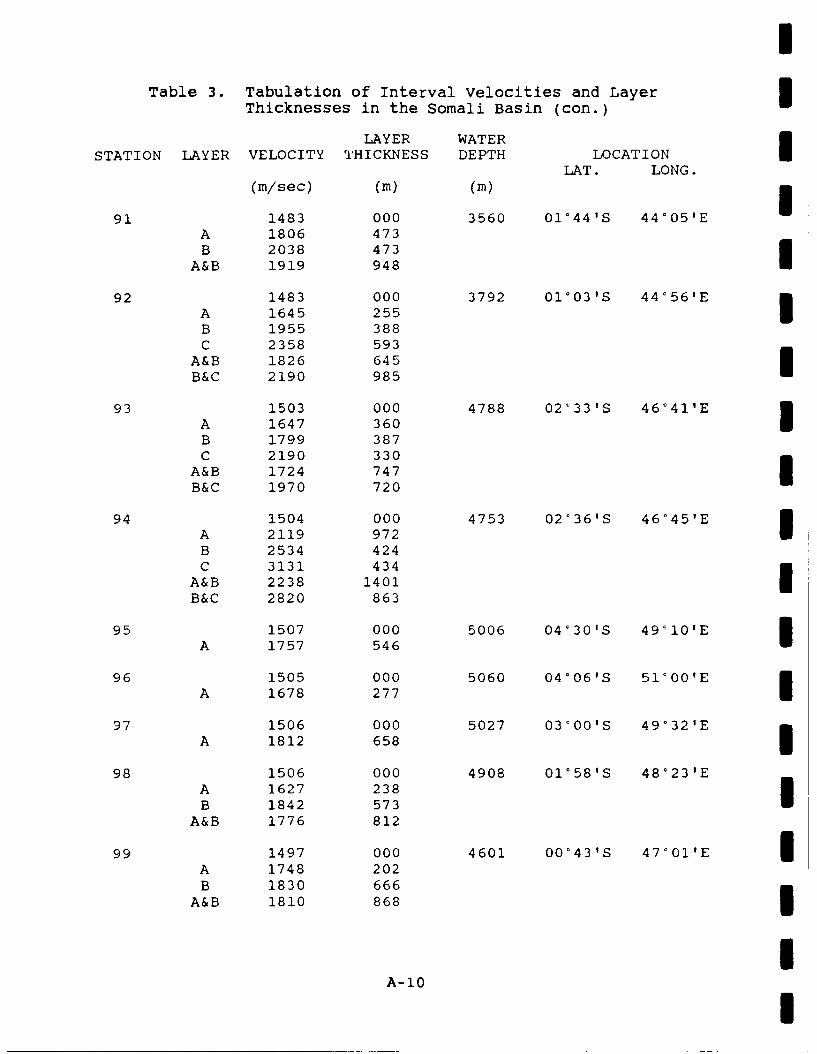
ITable 3. Tabulation of Interval Velocities and Layer
Thicknesses in the Somali Basin (con.)
LAYER WATER
STATION LAYER VELOCITY THICKNESS DEPTH LOCATIONLAT. LONG.
(m/sec) (M) (M)
91 1483 000 3560 01°44'S 44'05'EA 1806 473B 2038 473
A&B 1919 948
92 1483 000 3792 01°03'S 44°56'EA 1645 255B 1955 388C 2358 593
A&B 1826 645B&C 2190 985
93 1503 000 4788 02'33'S 46°41'EA 1647 360B 1799 387C 2190 330
A&B 1724 747B&C 1970 720
94 1504 000 4753 02'36'S 46°45'EA 2119 972B 2534 424C 3131 434
A&B 2238 1401B&C 2820 863
95 1507 000 5006 04'30'S 49'10'EA 1757 546
96 1505 000 5060 04°06'S 51'00'EA 1678 277
97 1506 000 5027 03'001S 49°32'EA 1812 658
98 1506 000 4908 01°58'S 48'23'EA 1627 238B 1842 573
A&B 1776 812
99 1497 000 4601 00'43'S 47°01'E IA 1748 202B 1830 666
A&B 1810 868
IA-10 I
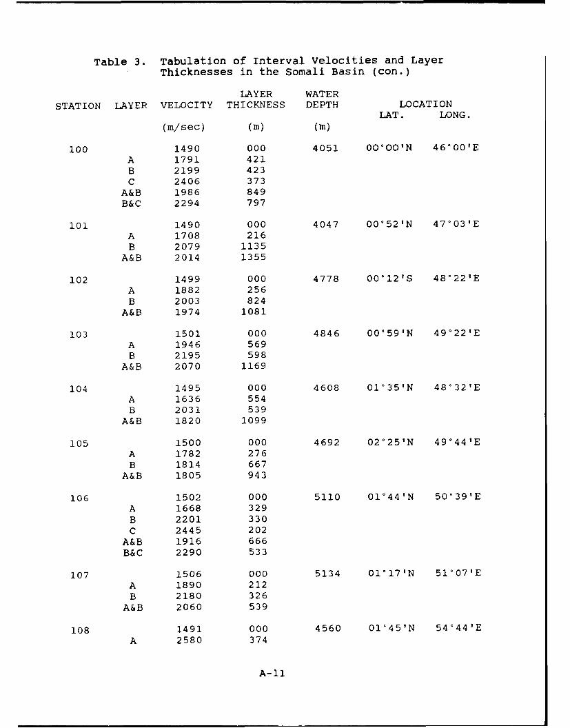
Table 3. Tabulation of Interval velocities and LayerThicknesses in the Somali Basin (con.)
LAYER WATERSTATION LAYER VELOCITY THICKNESS DEPTH LOCATION
LAT. LONG.(m/sec) (M) (M)
100 1490 000 4051 00 0 00'N 46° 0 0'EA 1791 421B 2199 423C 2406 373
A&B 1986 849B&C 2294 797
101 1490 000 4047 00°52'N 47'03'EA 1708 216B 2079 1135
A&B 2014 1355
102 1499 000 4778 00°12'S 48'22'EA 1882 256B 2003 824
A&B 1974 1081
103 1501 000 4846 00°59'N 49°22'EA 1946 569B 2195 598
A&B 2070 1169
104 1495 000 4608 01°35'N 48'32'EA 1636 554B 2031 539
A&B 1820 1099
105 1500 000 4692 02°25'N 49°44'EA 1782 276B 1814 667
A&B 1805 943
106 1502 000 5110 01°44'N 50'39'EA 1668 329B 2201 330C 2445 202
A&B 1916 666B&C 2290 533
107 1506 000 5134 01°17'N 51°07'EA 1890 212B 2180 326
A&B 2060 539
108 1491 000 4560 01'45'N 54'44'EA 2580 374
A-li
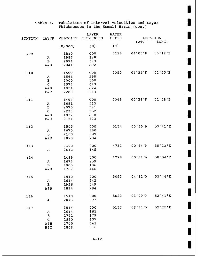
I
Table 3. Tabulation of Interval Velocities and Layer 3Thicknesses in the Somali Basin (con.)
LAYER WATERSTATION LAYER VELOCITY THICKNESS DEPTH LOCATION
LAT. LONG.(m/sec) (M) (M)
109 1510 000 5216 04'05'N 53'12'EA 1987 228B 2074 373
A&B 2041 602
110 1509 000 5080 04°34'N 52°35'EA 1566 258B 2000 560C 2574 643
A&B 1851 824B&C 2289 1213
ill 1498 000 5049 05'28'N 51°38'EA 1681 513B 2070 321C 2233 352
A&B 1822 838B&C 2154 673
112 1505 000 5134 05°36'N 53°41'EA 1670 380
B 2100 399A&B 1878 784
113 1490 000 4733 00°34'N 58'23'EA 1612 145
114 1489 000 4728 00°31'N 58°04'EA 1674 259B 1905 186
A&B 1767 446
115 1510 000 5093 04'12'N 53°44'EA 1614 242B 1926 549
A&B 1824 794
116 1510 000 5023 03o09,N 52o41,E 3A 2073 297
117 1514 000 5132 02°31'N 52'25'E IA 1614 161B 1791 179C 1830 137
A&B 1705 341B&C 1808 316
A-12 I
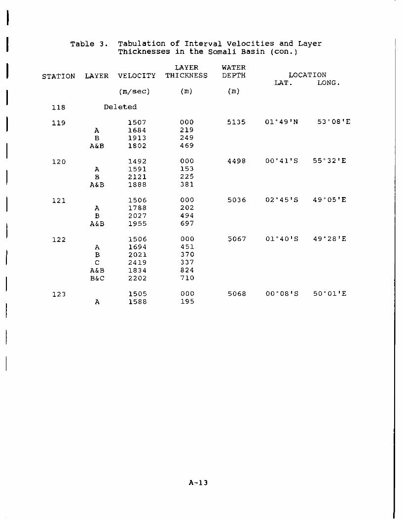
I
Table 3. Tabulation of Interval Velocities and LayerThicknesses in the Somali Basin (con.)
LAYER WATER
STATION LAYER VELOCITY THICKNESS DEPTH LOCATIONLAT. LONG.
(m/sec) (m) (m)
118 Deleted
119 1507 000 5135 01°49'N 53'08'EA 1684 219B 1913 249
A&B 1802 469
120 1492 000 4498 00'41'S 55°32'EA 1591 153B 2121 225
A&B 1888 381
121 1506 000 5036 02'451S 49'05'EA 1788 202B 2027 494
A&B 1955 697
122 1506 000 5067 01'401S 49°28'EA 1694 451B 2021 370C 2419 337
A&B 1834 824B&C 2202 710
123 1505 000 5068 00008'S 50*01'EA 1588 195
A-13
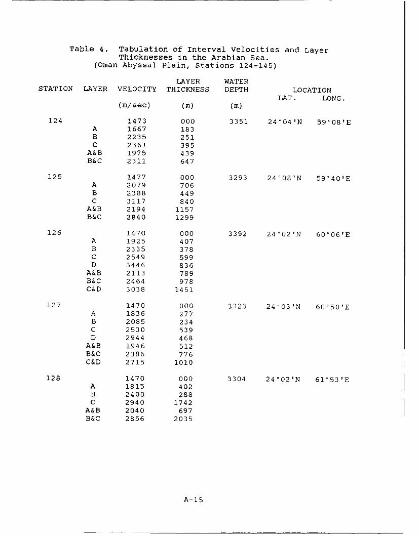
Table 4. Tabulation of Interval Velocities and LayerThicknesses in the Arabian Sea.
(Oman Abyssal Plain, Stations 124-145)
LAYER WATERSTATION LAYER VELOCITY THICKNESS DEPTH LOCATION
LAT. LONG.(m/sec) (M) (m)
124 1473 000 3351 24'04'N 59'081EA 1667 183B 2235 251C 2361 395
A&B 1975 439B&C 2311 647
125 1477 000 3293 24'08'N 59'401EA 2079 706B 2388 449C 3117 840
A&B 2194 1157B&C 2840 1299
126 1470 000 3392 24'021N 60 0 061EA 1925 407B 2335 378C 2549 599D 3446 836
A&B 2113 789B&C 2464 978C&D 3038 1451
127 1470 000 3323 24'03'N 60'501EA 1836 277B 2085 234C 2530 539D 2944 468
A&B 1946 512B&C 2386 776C&D 2715 1010
128 1470 000 3304 24'02'N 61'53,EA 1815 402B 2400 288C 2940 1742
A&B 2040 697B&C 2856 2035
A-15
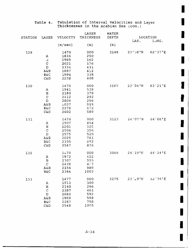
I
Table 4. Tabulation of Interval Velocities and LayerThicknesses in the Arabian Sea (con.)
LAYER WATERSTATION LAYER VELOCITY THICKNESS DEPTH LOCATIONLAr. LJNG.
(m/sec) (M) (M)
129 1470 000 3248 23°58'N 62°37'EA 1836 2503 1969 162C 2021 176
D 2334 431A&B 1887 412B&C 1996 338C&D 2238 608
130 1470 000 3169 23'56'N 63c21'EA 1941 538B 2180 379C 2412 292D 2804 296
A&B 4037 919B&C 2278 672C&D 2602 589
131 1470 000 3123 24'07'N 64'08'EA 1907 454B 2201 325C 2506 356D 2575 520
A&B 2025 781B&C 2355 612C&D 2547 876
132 1,i70 000 3066 24:19'N 64-34'EA 1972 422B 2307 555C 2438 447
A&B 2156 980B&C 2364 1003
133 1477 000 3275 23d9'N 62'36'EA 1813 300B 2140 296 IC 2387 461D 2680 592
A&B 1969 598B&C 2287 758C&D 2548 1055
II
A-16 I
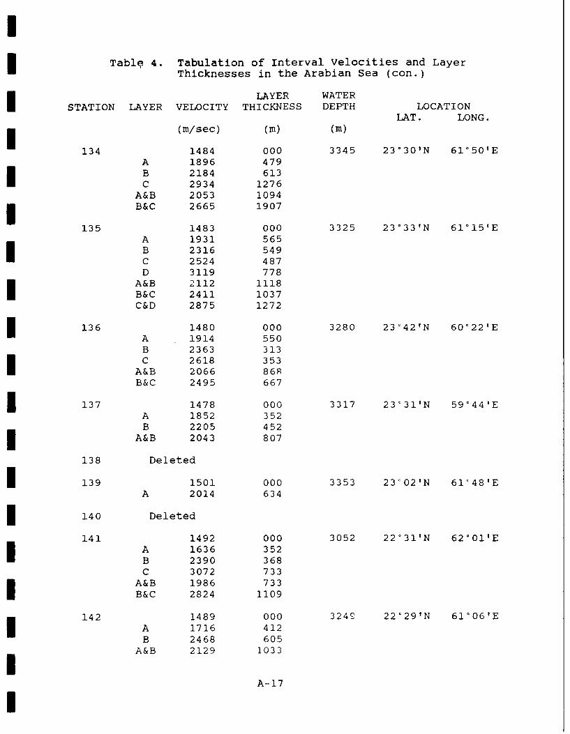
Tablp 4. Tabulation of Interval Velocities and LayerThicknesses in the Arabian Sea (con.)
LAYER WATERSTATION LAYER VELOCITY THICKNESS DEPTH LOCATION
LAT. LONG.(m/sec) (M) (M)
134 1484 000 3345 23'30'N 61'50'EA 1896 479B 2184 613C 2934 1276
A&B 2053 1094B&C 2665 1907
135 1483 000 3325 23°33'N 61'15'EA 1931 565B 2316 549C 2524 487D 3119 778
A&B 2112 1118B&C 2411 1037C&D 2875 1272
136 1480 000 3280 23'42'N 60'22'EA 1914 550B 2363 313C 2618 353
A&B 2066 868B&C 2495 667
137 1478 000 3317 23c31 1 N 59°44'EA 1852 352B 2205 452
A&B 2043 807
138 Deleted
139 1501 000 3353 23'02'N 61'48 1 EA 2014 634
140 Deleted
141 1492 000 3052 22°31'N 62°01'EA 1636 352B 2390 368C 3072 733
A&B 1986 733B&C 2824 1109
142 1489 000 3244 22°29'N 61'06'EA 1716 412B 2468 605
A&B 2129 1033
A-17
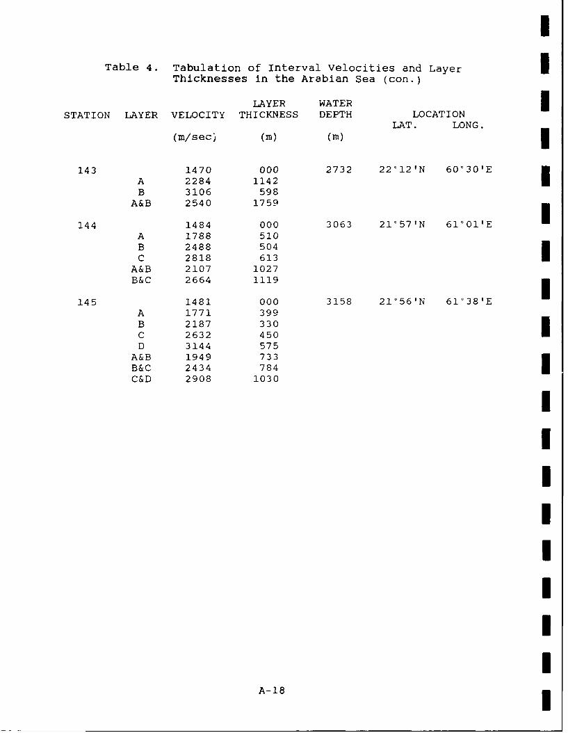
I
Table 4. Tabulation of Interval Velocities and Layer iThicknesses in the Arabian Sea (con.)
LAYER WATERSTATION LAYER VELOCITY THICKNESS DEPTH LOCATION
LAT. LONG.(m/sec (M) (M)i
143 1470 000 2732 22'12'N 60'30'EA 2284 1142B 3106 598
A&B 2540 1759
144 1484 000 3063 21'57'N 61°01'EA 1788 510B 2488 504C 2818 613
A&B 2107 1027B&C 2664 1119
145 1481 000 3158 21'56'N 61*38'EA 1771 399B 2187 330C 2632 450D 3144 575
A&B 1949 733B&C 2434 784C&D 2908 1030
iIIiii
IA-18I

Table 4. Tabulation of Interval Velocities and LayerThicknesses in the Arabian Sea (con.)
(OWENS Abyssal Plain, Stations 167, 168, 169, 170, 180, 181)
LAYER WATERSTATION LAYER VELOCITY THICKNESS DEPTH LOCATIONSLAT. LONG.
(m/sec) (M) (M)
167 1481 000 3258 21°29'N 61°17'EA 1690 181B 1877 246
C 2288 332j D 2623 289E 3363 2044
A&B 1795 427B&C 2103 580C&D 2438 622D&E 3260 2341
168 1481 000 3289 21'12'N 60°47'EA 1602 235B 2137 401C 2318 287D 2737 475E 3467 1774
A&B 1921 641B&C 2211 689C&D 2570 765D&E 3298 2259
169 1483 000 3398 20'41'N 60'29'EA 1562 255B 1995 315C 2513 285D 2737 374
A&B 1788 575B&C 2227 605C&D 2637 659
170 1480 000 3446 20°17'N 60'30'EA 1665 311B 2108 318C 2512 392
A&B 1876 634B&C 2322 713
A-19
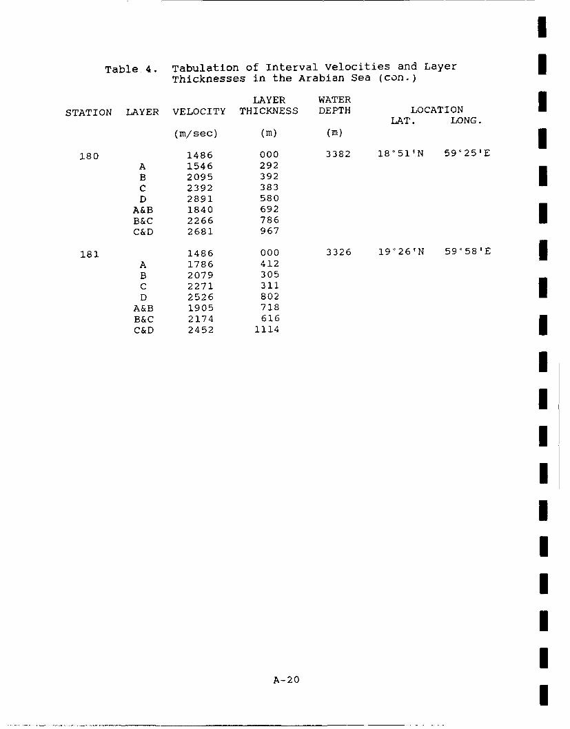
l
Table 4. Tabulation of Interval Velocities and Layer iThicknesses in the Arabian Sea (con.)
LAYER WATER ISTATION LAYER VELOCITY THICKNESS DEPTH LOCATION
LAT. LONG.
(m/sec) (M) (M)
180 1486 000 3382 18°51'N 59°25'EA 1546 292B 2095 392C 2392 383D 2891 580
A&B 1840 692B&C 2266 786C&D 2681 967
181 1486 000 3326 19'26'N 59°58'EA 1786 412B 2079 305C 2271 311D 2526 802
A&B 1905 718B&C 2174 616C&D 2452 1114
IIIIIIII
A- 20 I
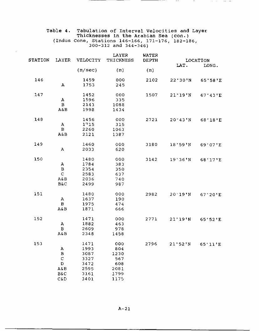
Table 4. Tabulation of Interval Velocities and LayerThicknesses in the Arabian Sea (con.)
(Indus Cone, Stations 146-166, 171-176, 182-186,300-312 and 344-346)
LAYER WATERSTATION LAYER VELOCITY THICKNESS DEPTH LOCATION
LAT. LONG.(m/sec) (M) (M)
146 1459 000 2102 22°30'N 65°58'EA 1753 245
147 1452 000 1507 21°19'N 67°43'EA 1596 335B 2143 1088
A&B 1998 1434
148 1456 000 2721 20'43'N 68'181EA 1715 315B 2260 1063
A&B 2121 1387
149 1460 000 3180 18'59'N 69'071EA 2033 620
150 1480 000 3142 19'36 1 N 68'17'EA 1784 383B 2354 350C 2583 637
A&B 2036 740B&C 2499 987
151 1480 000 2982 20'19'N 67'20'EA 1637 190B 1975 474
A&B 1871 666
152 1471 000 2771 21'19'N 65'52'EA 1882 463B 2609 978
A&B 2348 1458
153 1471 000 2796 21°52'N 6511'EA 1993 804B 3087 1230C 3327 567D 3472 608
A&B 2595 2081B&C 3161 1799C&D 3401 1175
A-21

I
Table 4. Tabulation of Interval Velocities and Layer IThicknesses in the Arabian Sea (con.)
LAYER WATERSTATION LAYER VELOCITY THICKNESS DEPTH LOCATION
LAT. LONG.(m/sec) (M) (M)
154 1482 000 3300 21°24'N 64°27'EA 1635 229B 2080 260C 2820 903D 3064 881
A&B 1858 492 IB&C 2634 1172C&D 2938 1785
155 1479 000 2893 20'43'N 65'23'E IA 2022 743B 2769 487
A&B 2291 1245
156 1476 000 2639 19'56'N 66°29'EA 1787 380B 2392 493C 2542 544D 3151 1276
A&B 2107 882B&C 2470 1037C&D 2955 1829
157 1471 000 3003 19'341N 67'061E IA 1660 168B 2008 252C 2451 611D 3224 941
A&B 1861 421B&C 2312 867C&D 2905 1567
158 1470 000 3311 18°31'N 68°29'EA 1606 168B 1957 281C 2298 299
A&B 1818 451B&C 2126 581
159 1468 000 3347 17'44'N 69'22'EA 1469 207B 1714 216C 2199 227
A&B 1589 424B&C 1947 446
IA-22I
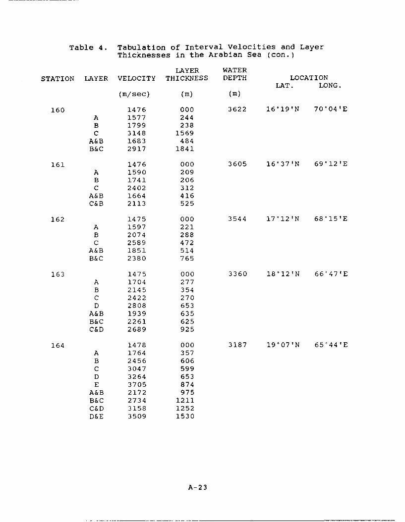
Table 4. Tabulation of Interval Velocities and LayerThicknesses in the Arabian Sea (con.)
LAYER WATERSTATION LAYER VELOCITY THICKNESS DEPTH LOCATION
LAT. LONG.(m/sec) (M) (M)
160 1476 000 3622 16°19'N 70°04'EA 1577 244B 1799 238C 3148 1569
A&B 1683 484B&C 2917 1841
161 1476 000 3605 16°37'N 69'12'EA 1590 209B 1741 206C 2402 312
A&B 1664 416C&B 2113 525
162 1475 000 3544 17'12'N 68'15'EA 1597 221B 2074 288C 2589 472
A&B 1851 514B&C 2380 765
163 1475 000 3360 18'12'N 66'47'EA 1704 277B 2145 354C 2422 270D 2808 653
A&B 1939 635B&C 2261 625C&D 2689 925
164 1478 000 3187 19'07'N 65'44'EA 1764 357B 2456 606C 3047 599D 3264 653E 3705 874
A&B 2172 975B&C 2734 1211C&D 3158 1252D&E 3509 1530
A-23
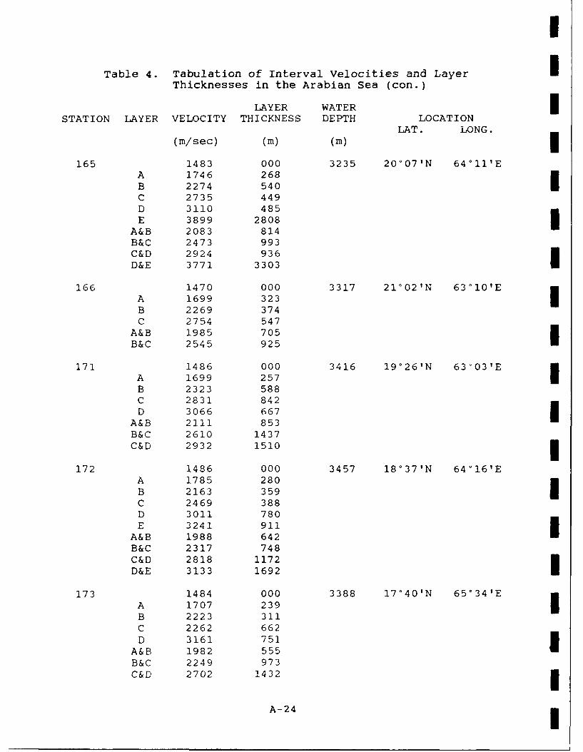
I
Table 4. Tabulation of Interval Velocities and Layer IThicknesses in the Arabian Sea (con.)
LAYER WATERSTATION LAYER VELOCITY THICKNESS DEPTH LOCATION
LAT. LONG.(m/sec) (M) (M) 3
165 1483 000 3235 20'07'N 64°11'EA 1746 268B 2274 540C 2735 449D 3110 485E 3899 2808
A&B 2083 814B&C 2473 993C&D 2924 936D&E 3771 3303
166 1470 000 3317 21°02'N 63°10'EA 1699 323B 2269 374
C 2754 547A&B 1985 705B&C 2545 925
171 1486 000 3416 19'26'N 63'03'EA 1699 257B 2323 588C 2831 842D 3066 667
A&B 2111 853B&C 2610 1437C&D 2932 1510 3
172 1486 000 3457 18'37'N 64'16'EA 1785 280B 2163 359C 2469 388D 3011 780E 3241 911
A&B 1988 642B&C 2317 748C&D 2818 1172D&E 3133 1692
173 1484 000 3388 17°40'N 65°34'EA 1707 239B 2223 311C 2262 662D 3161 751
A&B 1982 555B&C 2249 973C&D 2702 1432
A-24
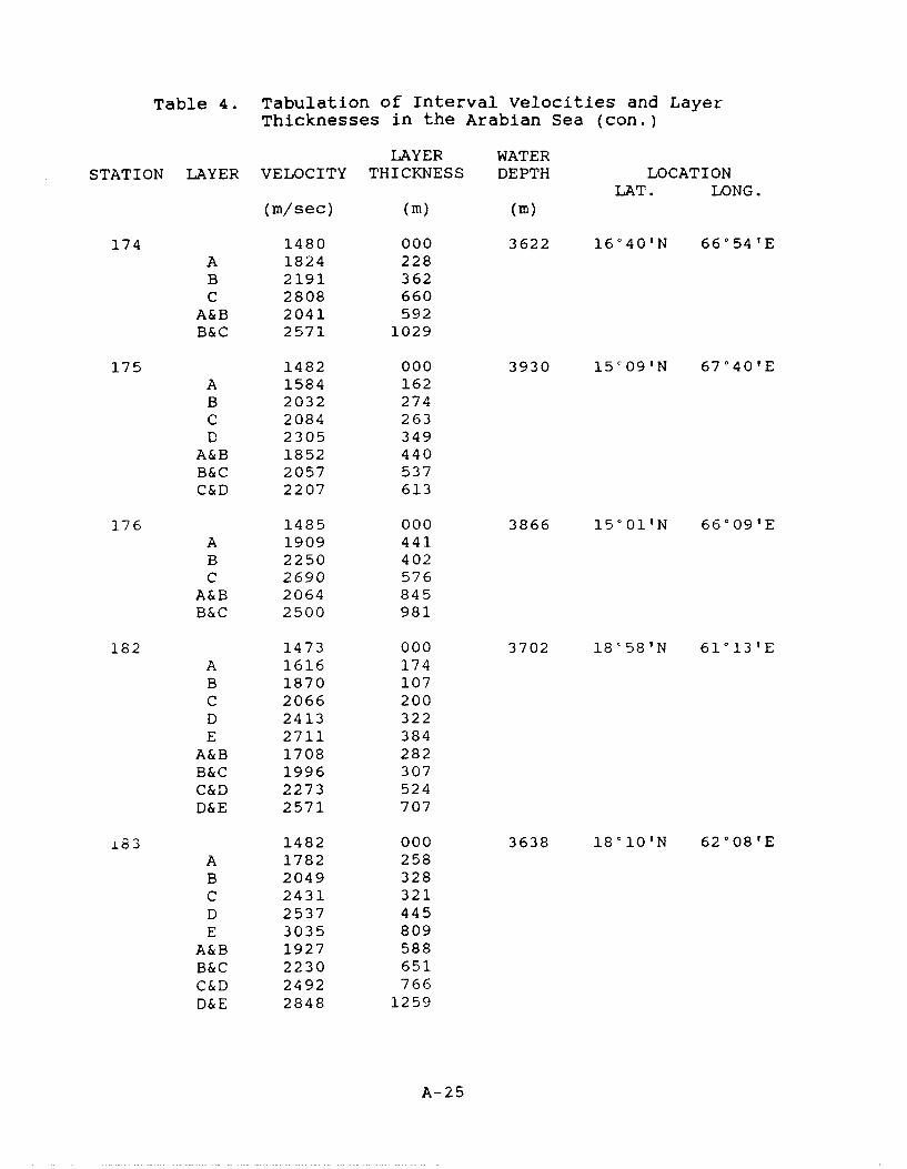
Table 4. Tabulation of Interval Velocities and LayerThicknesses in the Arabian Sea (con.)
LAYER WATERSTATION LAYER VELOCITY THICKNESS DEPTH LOCATION
LAT. LONG.(m/sec) (M) (M)
174 1480 000 3622 16'40'N 66°54'EA 1824 228B 2191 362C 2808 660
A&B 2041 592B&C 2571 1029
175 1482 000 3930 15'091N 67'40'EA 1584 162B 2032 274C 2084 263D 2305 349
A&B 1852 440B&C 2057 537C&D 2207 613
176 1485 000 3866 15'01'N 66°09'EA 1909 441B 2250 402C 2690 576
A&B 2064 845B&C 2500 981
182 1473 000 3702 18C58 1 N 61'13'EA 1616 174B 1870 107C 2066 200D 2413 322E 2711 384
A&B 1708 282B&C 1996 307C&D 2273 524D&E 2571 707
±83 1482 000 3638 18°10'N 62'08'EA 1782 258B 2049 328C 2431 321D 2537 445E 3035 809
A&B 1927 588B&C 2230 651C&D 2492 766D&E 2848 1259
A-25
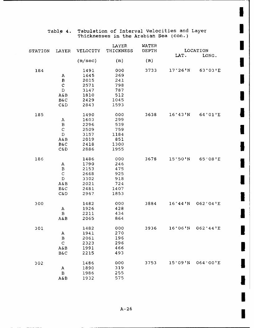
i
Table 4. Tabulation of Interval Velocities and Layer iThicknesses in the Arabian Sea (con.)
LAYER WATERSTATION LAYER VELOCITY THICKNESS DEPTH LOCATION
LAT. LONG.
(m/sec) (M) (M)
184 1491 000 3733 17'26'N 63°03'EA 1645 269B 2015 241C 2571 798D 3147 787
A&B 1810 512B&C 2429 1045C&D 2843 1593
185 1490 000 3638 16'43'N 64°01'E 1A 1603 299B 2296 539C 2509 759D 3157 1184
A&B 2019 851B&C 2418 1300C&D 2886 1955
186 1486 000 3678 15*50'N 65'08'EA 17-90 246B 2153 475
C 2668 925D 3302 918
A&B 2021 724B&C 2481 1407C&D 2967 1853 i
300 1482 000 3884 16'44'N 062*04'EA 1926 428B 2211 434
A&B 2065 864
301 1482 000 3936 16°06'N 062'44'EA 1941 270 IB 2061 196C 2323 296
A&B 1991 466B&C 2215 493
302 1486 000 3753 15'09'N 064° 0 00'EA 1890 319 IB 1986 255
A&B 1932 575 1
iA-26
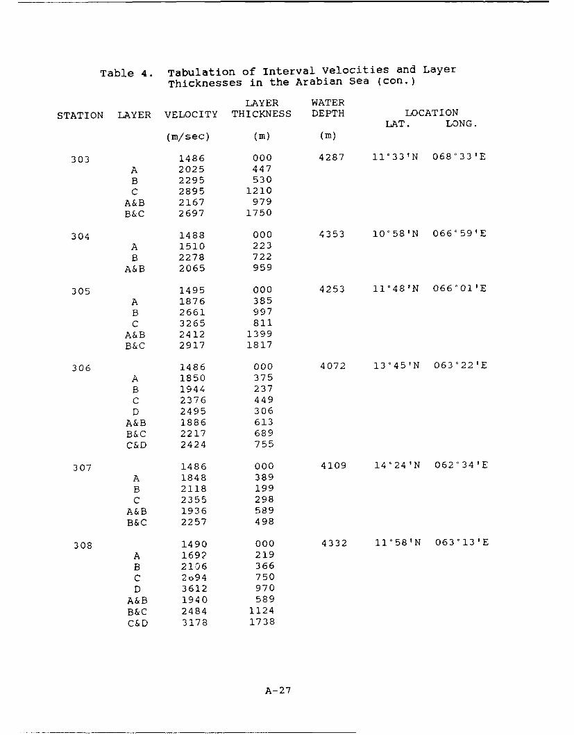
Table 4. Tabulation of Interval Velocities and LayerThicknesses in the Arabian Sea (con.)
LAYER WATERSTATION LAYER VELOCITY THICKNESS DEPTH LOCATION
LAT. LONG.
(m/sec) (M) (M)
303 1486 000 4287 1133'N 068°33'E
A 2025 447B 2295 530C 2895 1210
A&B 2167 979B&C 2697 1750
304 1488 000 4353 10'58'N 066'59'E
A 1510 223B 2278 722
A&B 2065 959
305 1495 000 4253 11481N 066'01'E
A 1876 385B 2661 997C 3265 811
A&B 2412 1399B&C 2917 1817
306 1486 000 4072 13'45'N 063°22'E
A 1850 375B 1944 237C 2376 449D 2495 306
A&B 1886 613B&C 2217 689C&D 2424 755
307 1486 000 4109 14'24'N 062°34'E
A 1848 389B 2118 199C 2355 298
A&B 1936 589B&C 2257 498
308 1490 000 4332 1158'N 063'13'E
A 1692 219B 2106 366C 2o94 750D 3612 970
A&B 1940 589B&C 2484 1124
C&D 3178 1738
A-27
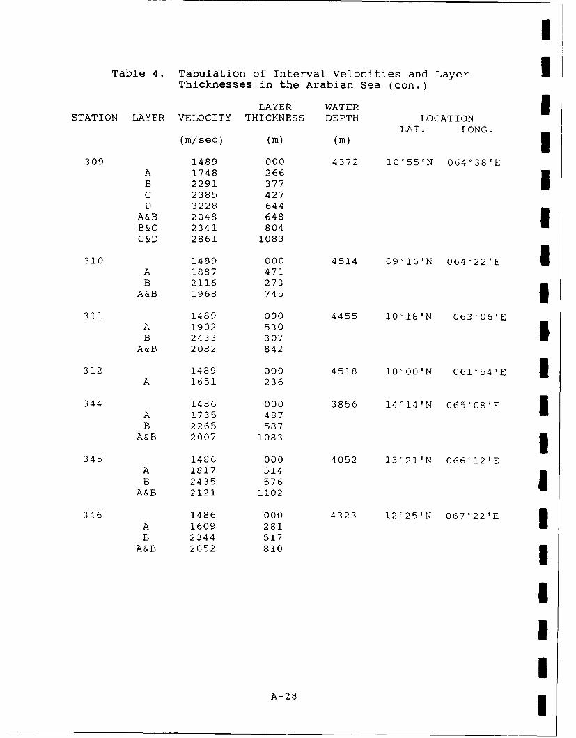
I
Table 4. Tabulation of Interval velocities and Layer IThicknesses in the Arabian Sea (con.)
LAYER WATERSTATION LAYER VELOCITY THICKNESS DEPTH LOCATION
LAT. LONG.(m/sec) (M) (M)
309 1489 000 4372 10'551N 064°381EA 1748 266B 2291 377C 2385 427D 3228 644
A&B 2048 648B&C 2341 804C&D 2861 1083
310 1489 000 4514 C9°16'N 064'22'E IA 1887 471B 2116 273
A&B 1968 745
311 1489 000 4455 10'18'N 063-061EA 1902 530B 2433 307
A&B 2082 842
312 1489 000 4518 10'00'N 061'54'E 5A 1651 236
344 1486 000 3856 14'14'N 065'08 1 EA 1735 487B 2265 587
A&B 2007 1083 1345 1486 000 4052 13'21'N 066:12'E
A 1817 514B 2435 576
A&B 2121 1102
346 1486 000 4323 12c25'N 067'22 1 EA 1609 281B 2344 517
A&B 2052 810 3
III
A-28 3
IIIIIIII APPENDIX B
CORE VELOCITY CORRECTION PROCEDURES
II1IIIIIII* B-i
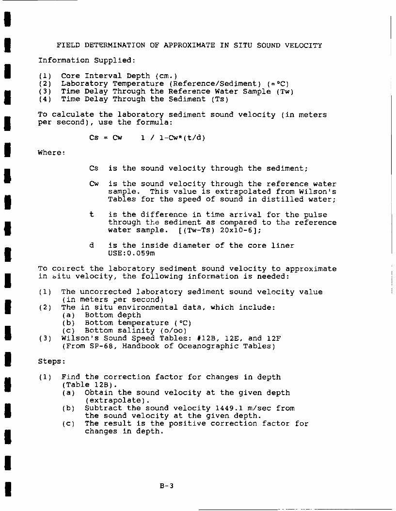
FIELD DETERMINATION OF APPROXIMATE IN SITU SOUND VELOCITY
Information Supplied:
(1) Core Interval Depth (cm.)(2) Laboratory Temperature (Reference/Sediment) (=°C)(3) Time Delay Through the Reference Water Sample (Tw)(4) Time Delay Through the Sediment (Ts)
To calculate the laboratory sediment sound velocity (in metersper second), use the formula:
Cs = Cw 1 / 1-Cw*(t/d)
Where:
Cs is the sound velocity through the sediment;
Cw is the sound velocity through the reference watersample. This value is extrapolated from Wilson'sTables for the speed of sound in distilled water;
t is the difference in time arrival for the pulsethrough the sediment as compared to the referencewater sample. [(Tw-Ts) 20x10-6];
d is the inside diameter of the core linerUSE:0.059m
To correct the laboratory sediment sound velocity to approximatein 6itu velocity, the following information is needed:
(1) The uncorrected laboratory sediment sound velocity value(in meters ?er second)
(2) The in situ environmental data, which include:(a) Bottom depth(b) Bottom temperature (°C)(c) Bottom salinity (o/oo)(3) Wilson's Sound Speed Tables: #12B, 12E, and 12F(From SP-68, Handbook of Oceanographic Tables)
Steps:
(1) Find the correction factor for changes in depth(Table 12B).(a) Obtain the sound velocity at the given depth
(extrapolate).(b) Subtract the sound velocity 1449.1 m/sec from
the sound velocity at the given depth.(c) The result is the positive correction factor for
changes in depth.
B-3
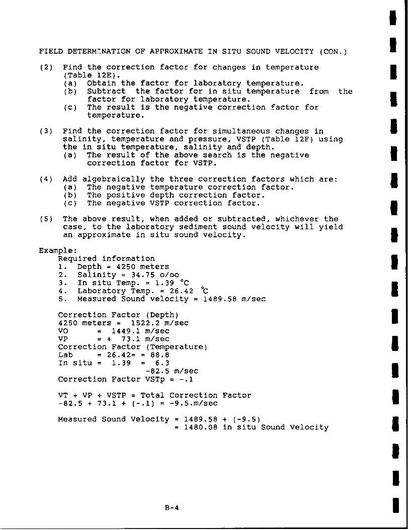
I
FIELD DETERMWNATION OF APPROXIMATE IN SITU SOUND VELOCITY (CON.) i(2) Find the correction factor for changes in temperature
(Table 12E).(a) Obtain the factor for laboratory temperature.(b) Subtract the factor for in situ temperature from the
factor for laboratory temperature. I(c) The result is the negative correction factor for
temperature.
(3) Find the correction factor for simultaneous changes in Isalinity, temperature and pressure, VSTP (Table 12F) usingthe in situ temperature, salinity and depth.(a) The result of the above search is the negative I
correction factor for VSTP.
(4) Add algebraically the three correction factors which are:(a) The negative temperature correction factor.(b) The positive depth correction factor.(c) The negative VSTP correction factor. 3
(5) The above result, when added or subtracted, whichever thecase, to the laboratory sediment sound velocity will yieldan approximate in situ sound velocity.
Example:Required information1. Depth = 4250 meters2. Salinity = 34.75 o/oo3. In situ Temp. = 1.39 0C4. Laboratory Temp. = 26.42 nC5. Measured Sound velocity = 1489.58 m/sec
Correction Factor (Depth)4250 meters = 1522.2 m/sec iVO = 1449.1 m/secVP = + 73.1 m/secCorrection Factor (Temperature) ILab = 26.42= = 88.8In situ = 1.39 = 6.3
-82.5 m/sec 3Correction Factor VSTp = -.1
VT + VP + VSTP = Total Correction Factor-82.5 + 73.1 + (-.1) = -9.5.m/sec
Measured Sound Velocity = 1489.58 + (-9.5)= 1480.08 in situ Sound Velocity
I
B-4 i
LABORATORY DETERMINATION OF IN SITU SOUND VELOCITY
COMPRESSIONAL WAVE VELOCITY
Descriptions which delineate sediment boundary layers are ob-served from X-radiographs of the core. Each core is analyzed forcompressional wave velocity (sound velocity) at the sedimentboundary layers.
An underwater sediment velocimeter measures the time required fora 400-Hz signal to travel through the core liner thickness at thetransiting crystal, travel through the sediment thickness, andtravel through the core liner at the receiving crystal. Anothertime delay measurement (900 to the axis of the first time delaymeasurement) is taken so that sound velocity changes caused bygrain orientation will be detected. Similar time delay measure-ments are noted for a distilled water reference standard.
The time delay difference between the reference standard and thesediment is calculated for each sub-sampling interval within thecore. This difference is needed to calculate the sound velocityusing Wilson's equations for computing the speed of sound in sea-water.
In situ salinity (in parts per thousand), in situ temperature (in0 C), and water column depth (in meters) values are either di-rectly measured by field surveys or obtained from historicaldatabase records. Salinity, temperature, and pressure correctionfactors are calculated using a modified version of Wilson'sequations.
The sound velocity of the bottom water is calculate, from therelationship:
CWB=1449.1+VP2+VS2+VT2+VSTP2)*3.28083
Equation terms are identical to those used by Wilson with theexception of CWB. This term combines Wilson's use of the letter"C" to denote sound velocity with the letter "W" to denote"water", and the letter "B" to denote "bottom".
Sediment sound velocity is calculated from an enhanced version of
the Mandex, Incorporated velocity calculation formula:
Cs = Cw * 1/1-Cw *(T/D)
where:Cs = Sound velocity through sediment (M/Sec.)Cw = Sound velocity through distilled water (M/Sec.)T = Difference in arrival time for the pulse through
sediment as compared to the reference standard.D = Inside diameter of the core tube (M.)
B-5
I
The enhanced version adjusts the sound velocity for temperature, Ipressure, and salinity conditions. Sediment interstitialsalinity is assumed to be identical to the water in situ salini-ty. The sediment core and distilled water reference standardsare allowed to reach ambient temperature conditions (usually an8-hour equilibrium period) prior to time delay measurements. Thepressure correction factor is reflected in Wilson's equations. 3A graphical representation of the average sound velocity varia-tions within the core is generated with a tabular listing whichshows each plane's sediment sound velocity and the average of thetwo planes.
A discrete average and a weighted average tabular listing whichalso indicates the sediment/water velocity ratio is included whenit is requested by the user community.
IIi
IiIIUIII
B-6 3
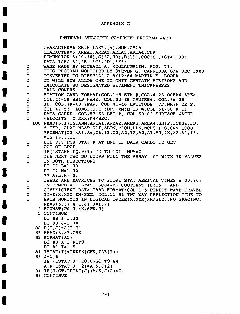
APPENDIX C
INTERVAL VELOCITY COMPUTER PROGRAM WABR
CHARACTER*6 SHIP,IAR*1(5),HORIZ*I6CHARACTER*5 AREAI,AREA2,AREA3,AREA4,CHKDIMENSION A(30,30),S(30,30),B(15),COC(8),ISTAT(30)DATA IAR/'A','B','C','D','E'/
C WABR MADE BY MICHAEL A. MCGLAUGHLIN, AUG. 79,C THIS PROGRAM MODIFIED BY STEVEN G. CARRUBBA O/A DEC 1983C CONVERTED TO DISSPLA9-0 6/12/84 MARTIN H. BOODAC IT WILL NOW ALLOW ONE TO OMIT CERTAIN HORIZONS ANDC CALCULATE SO DESIGNATED SEDIMENT THICKNESSES
CALL COMPRSC STATION CARD FORMAT:COL.1-3 STA.#,COL.4-23 OCEAN AREA,C COL.24-29 SHIP NAME, COL.30-35 CRUISE#, COL.36-38C JD, COL.39-40 YEAR, COL.41-46 LATITUDE (DD.MM)N OR S,C COL.47-53 LONGITUDE (DDD.MM)E OR W,COL.54-56 # OFC DATA CARDS, COL.57-58 LEG #, COL.59-63 SURFACE WATERC VELOCITY (X.XXX)KM/SEC.
100 READ(5,1)ISTANM,AREA1,AREA2,AREA3,AREA4,SHIP,ICRUZ,JD,* IYR, ALAT,MLAT,DLT,ALON,MLON,DLN,NCDS,LEG,SWV,ICOU 1*FORMAT(I3,4A5,A6,I6,I3,I2,A2,1X,A2,AI,A3,1X,A2,AI,I3,*12,F5.3,II)
C USE 999 FOR STA. # AT END OF DATA CARDS TO GETC OUT OF LOOP
IF(ISTANM.EQ.999) GO TO 101 NUM=0C THE NEXT TWO DO LOOPS FILL THE ARRAY "A" WITH 30 VALUESC IN BOTH DIRECTIONS
DO 77 L=1,30DO 77 M=1,3077 A(L,M)=0.
C THESE ARE MATRICES TO STORE STA. ARRIVAL TIMES A(30,30)C INTERMEDIATE LEAST SQUARES QUOTIENT (B(15)) ANDC COEFFICIENT DATA CARD FORMAT:COL.1-5 DIRECT WAVE TRAVELC TIME(X.XXX)KM/SEC. COL.11-31 TWO WAY REFLECTION TIME TOC EACH HORIZON IN LOGICAL ORDER(X.XXX)KM/SEC.,NO SPACING.
READ(5,3)(A(I,J),J=1,7)3 FORMAT(F6.3,4X,6F6.3)2 CONTINUE
DO 88 I=1,30DO 88 J=1,30
88 S(I,J)=A(I,J)85 READ(5,82)CHK82 FORMAT(A5)
DO 83 K=I,NCDSDO 81 I=1,5
81 ISTAT(I)=INDEX(CHK,IAR(I))83 J=1,5
IF (ISTAT(J).EQ.0)GO TO 84A(K,ISTAT(J)+2)=A(K,J+2)
84 IF(J.GT.ISTAT(J))A(K,J+2)=0.83 CONTINUE
C-i
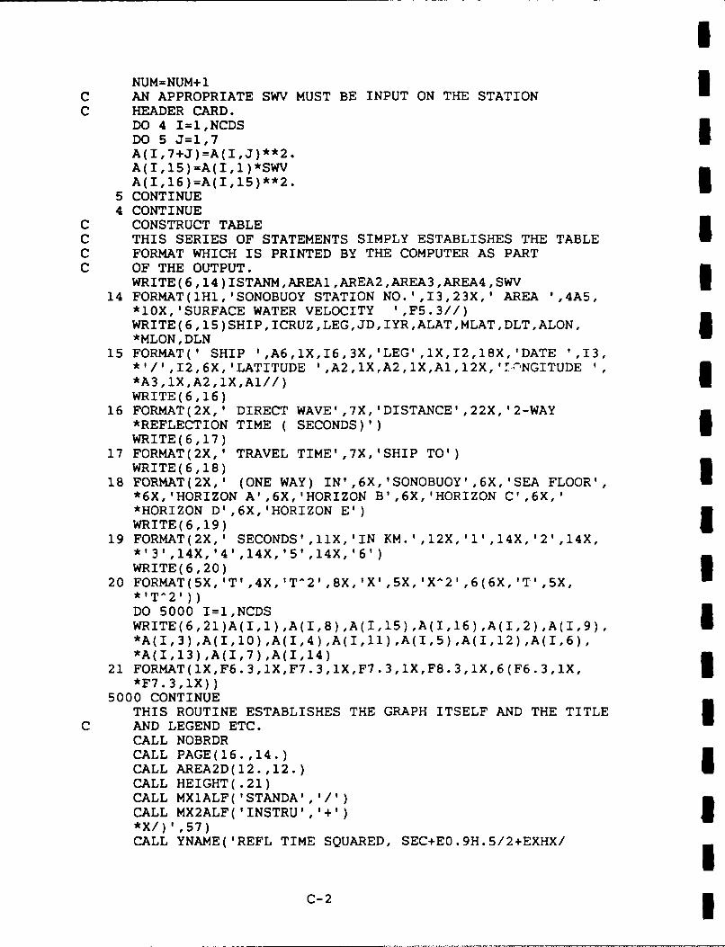
NUM=NUM+ 1C AN APPROPRIATE SWV MUST BE INPUT ON THE STATIONC HEADER CARD.
DO 4 I=1,NCDSDO 5 J=1,7I
A(I,7+J)=A(I,J)**2.
A(I,16 )=A(I,15)**2.5 CONTINUE4 CONTINUE
C CONSTRUCT TABLE
C THIS SERIES OF STATEMENTS SIMPLY ESTABLISHES THE TABLEC FORMAT WHICH IS PRINTED BY THE COMPUTER AS PARTC OF THE OUTPUT.
WRITE (6 ,14 )ISTANM ,AREA1 ,AREA2 ,AREA3 ,AREA4 ,SWVI14 FORMAT(1H1,'SONOBUOY STATION NO.1,I3,23X,' AREA ',4A5,
*10X,'SURFACE WATER VELOCITY ',F5.3//)
WRITE(6,15)SHIP,ICRUZ,LEG,JD,IYR,ALAT,MLAT,DLT,ALON,15 FORMT'SIP'AX163,LG,1,21X'DTN,315*ORAT' SH6XIP1ATIUD ,A2,16X,A2EG,lX,I1,18X,'DANGTDE ',13* A 3/ ' , 1 2 , 6 X , L T U D A l / / )A , X A 1 1 X 1 --- G I U E 1
WRITE(6,16)16 FORMAT(2X,' DIRECT WAVE' ,7X,-DISTANCE' ,22X,'2-WAY
*REFLECTION TIME ( SECONDS)')I
17 FORMAT(2X,' TRAVEL TIME',7X,'SHIP TO')WRITE(6,18)
I8 FORMAT(2X,' (ONE WAY) IN',6X,'SONOBUOY',6X,'SEA FLOOR',U*6X,'HORIZON A',6X,'HORIZON B',6X,'HORIZON C',6X,'*HORIZON D',6X,'HORIZON E-)
WRITE(6,19)19 FORMAT(2X,' SECONDS',11X,'IN KM.',12X,'1',14X,'2',14X,
*13' ,14X, '4' ,14X, '5' ,14X, '6')WRITE(6,20)
20 FORMAT(5X,'T',4X,'T-2',8X,'X',5X,'X^2',6(6X,'T',5X,*IT-2')
DO 5000 I=1,NCDSWRITE(6,21)A(I,1),A(I,8),A(I,15),A(I,16),A(I,2),A(I,9),*A(I,3),A(I,10),A(I,4),A(I,ll),A(I,5),A(I,12),A(I,6),*A(I,13),A(I,7),A(I,14)
21 FORMAT( 1X,F6. 3,1X,F7.3, 1X,F7.3 ,1X,F8.3, lX,6 (F6.3 ,1X,I
5000 CONTINU
THIS ROUTINE ESTABLISHES THE GRAPH ITSELF AND THE TITLEC AND LEGEND ETC.
CALL NOBRDRCALL PAGE(16.,14.)CALL AREA2D(12.,12.)ICALL HEIGHT(.21)CALL MX1ALF('STANDA','/')CALL MX2ALF('INSTRU','+'*X/)',51CALL YNAME('REFL TIME SQUARED, SEC+EO.9H.5/2+EXHX/
C- 23
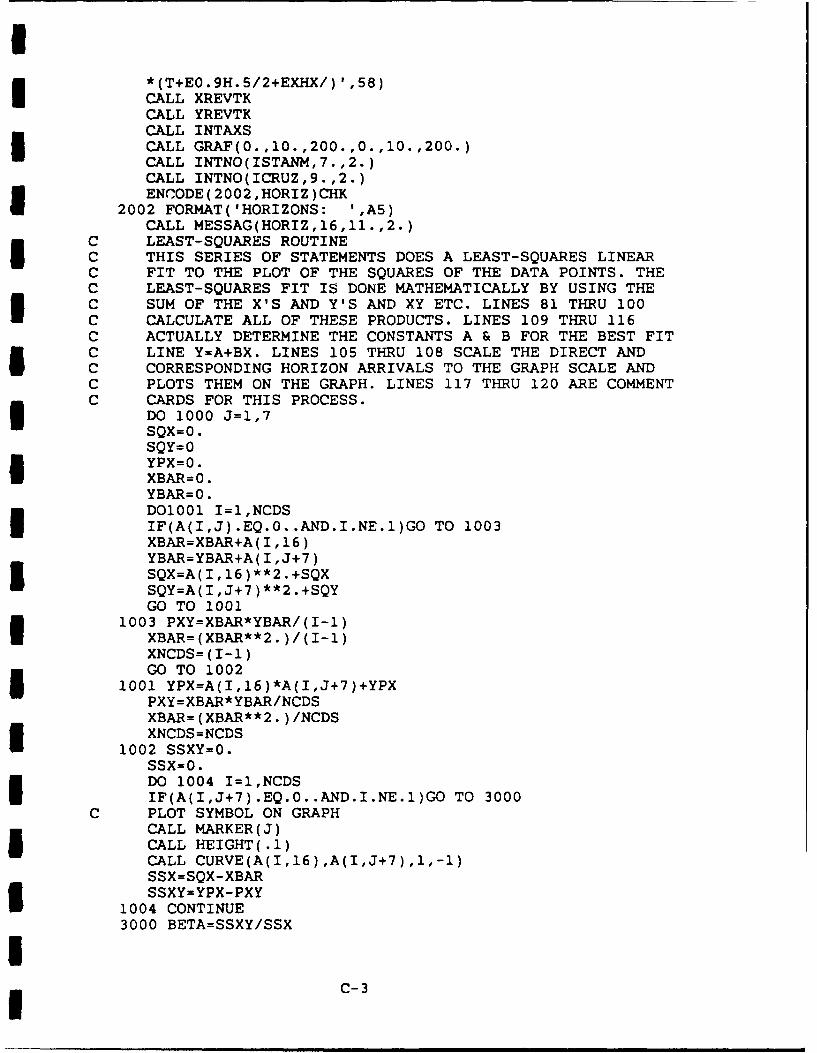
*(T+EO.9H.5/2+EXHX/)',58)CALL XREVTKCALL YREVTKCALL INTAXSCALL GRAF(0.,10.,200.,0.,10.,200.)CALL INTNO(ISTANM,7.,2.)CALL INTNO(ICRUZ,9.,2.)ENCODE(2002,HORIZ)CHK
2002 FORMAT('HORIZONS: ',A5)CALL MESSAG(HORIZ,16,11.,2.)
C LEAST-SQUARES ROUTINEC THIS SERIES OF STATEMENTS DOES A LEAST-SQUARES LINEARC FIT TO THE PLOT OF THE SQUARES OF THE DATA POINTS. THEC LEAST-SQUARES FIT IS DONE MATHEMATICALLY BY USING THEC SUM OF THE X'S AND Y'S AND XY ETC. LINES 81 THRU 100C CALCULATE ALL OF THESE PRODUCTS. LINES 109 THRU 116C ACTUALLY DETERMINE THE CONSTANTS A & B FOR THE BEST FITC LINE Y=A+BX. LINES 105 THRU 108 SCALE THE DIRECT ANDC CORRESPONDING HORIZON ARRIVALS TO THE GRAPH SCALE ANDC PLOTS THEM ON THE GRAPH. LINES 117 THRU 120 ARE COMMENTC CARDS FOR THIS PROCESS.
DO 1000 J=1,7SQX=o.SQY=0YPX=0.XBAR=0.YBAR=0.DO1001 I=1,NCDSIF(A(I,J).EQ.0..AND.I.NE.1)GO TO 1003XBAR=XBAR+A(I,16)YBAR=YBAR+A(I,J+7)SQX=A(I,16)**2.+SQXSQY=A(I,J+7)**2.+SQYGO TO 1001
1003 PXY=XBAR*YBAR/(I-1)XBAR=(XBAR**2.)/(I-1)XNCDS=(I-I)GO TO 1002
1001 YPX=A(I,16)*A(I,J+7)+YPXPXY=XBAR*YBAR/NCDSXBAR=(XBAR**2.)/NCDSXNCDS=NCDS
1002 SSXY=0.SSx=o.DO 1004 I=1,NCDSIF(A(I,J+7).EQ.0..AND.I.NE.1)GO TO 3000
C PLOT SYMBOL ON GRAPHCALL MARKER(J)CALL HEIGHT(.1)CALL CURVE(A(I,16),A(I,J+7),1,-I)SSX=SQX-XBARSSXY=YPX-PXY
1004 CONTINUE3000 BETA=SSXY/SSX
C-3
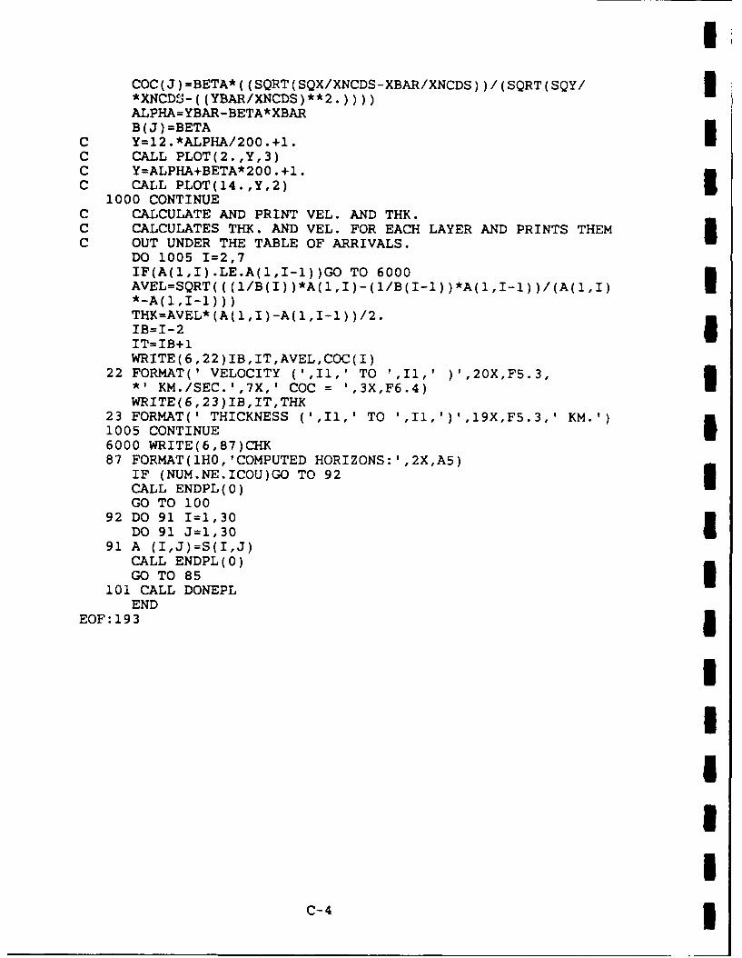
COC(J)=BETA*( (SQRT(SQX/XNCDS-XBAR/XNCDS) )/(SQRT(SQY/I
*yaNCDSj.( (YBAR/XNCDS)**2.))))ALPHA= YBAR- BETA* XBARB(J)=BETA
C Y=12.*ALPHA/200.+1.IC CALL PLOT(2.,Y,3)C Y=ALPHA+BETA*200. +1.C CALL PLOT(14.,Y,2)
1000 CONTINUEC CALCULATE AND PRINT VEL. AND THK.C CALCULATES THK. AND VEL. FOR EACH LAYER AND PRINTS THEMC OUT UNDER THE TABLE OF ARRIVALS.
DO 1005 I=2,7IF(A(1,I).LE.A(1,I-1))GO TO 6000
*-A(1,I..1))
IB=I-2IT=IB+1WRITE(6,22)IB,IT,AVEL,COC(I)
22 FORMAT(' VELOCITY (',I1,' TO ',I1,' )',20X,F5.3,*1 KM./SEC.',7X,' COC = 1,3X,F6.4)IWRITE(6 ,23)IB,IT,THK
23 FORMAT(' THICKNESS (1,11,' TO ',I1,')',19X,F5.3,' KM.')1005 CONTINUEI6000 WRITE(6,87)CHK87 FORMAT(1H0, 'COMPUTED HORIZONS: ',2X,A5)
IF (NUM.NE.ICOU)GO TO 92CALL ENDPL(0)GO TO 100
92 DO 91 I=1,30DO 91 J=1,30I
91 A (I,J)=S(I,J)CALL ENDPL(0)GO TO 85
101 CALL DONEPLEND
EOF: 1931
C- 41
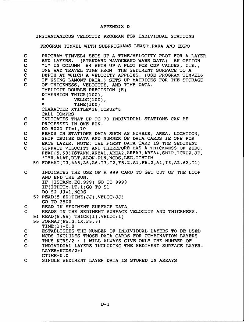
APPENDIX D
INSTANTANEOUS VELOCITY PROGRAM FOR INDIVIDUAL STATIONS
PROGRAM TIMVEL WITH SUBPROGRAMS LEAST,PARA AND EXPO
C PROGRAM TIMVEL4 SETS UP A TIME/VELOCITY PLOT FOR A LAYERC AND LAYERS. (STANDARD NAVOCEANO WABR DATA) AN OPTIONC "1" IN COLUMN 64 SETS UP A PLOT FOR CDP VALUES, I.E.,C ONE WAY TRAVEL TIME FROM THE SEDIMENT SURFACE TO AC DEPTH AT WHICH A VELOCITY APPLIES. (USE PROGRAM TIMVEL6C IF USING LAMONT DATA.) SETS UP MATRICES FOR THE STORAGEC OF THICKNESS, VELOCITY, AND TIME DATA.
IMPLICIT DOUBLE PRECISION (S)DIMENSION THICK(100),* VELOC(100),* TIME(100)
CHARACTER XTITLE*36,ICRUZ*6CALL COMPRS
C INDICATES THAT UP TO 70 INDIVIDUAL STATIONS CAN BEC PROCESSED IN ONE RUN.
DO 5000 II=1,70C READS IN STATIONS DATA SUCH AS NUMBER, AREA, LOCATION,C SHIP CRUISE DATA AND NUMBER OF DATA CARDS IE ONE FORC EACH LAYER. NOTE: THE FIRST DATA CARD IS THE SEDIMENTC SURFACE VELOCITY AND THEREFORE HAS A THICKNESS OF ZERO.
READ(5,50)ISTANM,AREA1,AREA2,AREA3,AREA4,SHIP,ICRUZ,JD,*IYR,ALAT,DLT,ALON,DLN,NCDS,LEG,ITHTIM
50 FORMAT(13,4A5,A6,A6,I3,I2,F5.2,AI,F6.2,AI,I3,A2,6X,II)
C INDICATES THE USE OF A 999 CARD TO GET OUT OF THE LOOPAND END THE RUN.IF (ISTANM.EQ.999) GO TO 9999IF(ITHTIM.LT.1)GO TO 51DO 52 JJ=1,NCDS
52 READ(5,60)TIME(JJ),VELOC(JJ)GO TO 2500
C READ IN SEDIMENT SURFACE DATAC READS IN THE SEDIMENT SURFACE VELOCITY AND THICKNESS.
51 READ(5,55) THICK(1),VELOC(1)55 FORMAT(F5.3,1X,F5.3)
TIME(1)=0.0C ESTABLISHES THE NUMBER OF INDIVIDUAL LAYERS TO BE USEDC NCDS INCLUDES THOSE DATA CARDS FOR COMBINATION LAYERSC THUS NCRS/2 + 1 WILL ALWAYS GIVE ONLY THE NUMBER OFC INDIVIDUAL LAYERS INCLUDING THE SEDIMENT SURFACE LAYER.
LAYER=NCDS/2+1CTIME=0.0
C SINGLE SEDIMENT LAYER DATA IS STORED IN ARRAYS
D-1
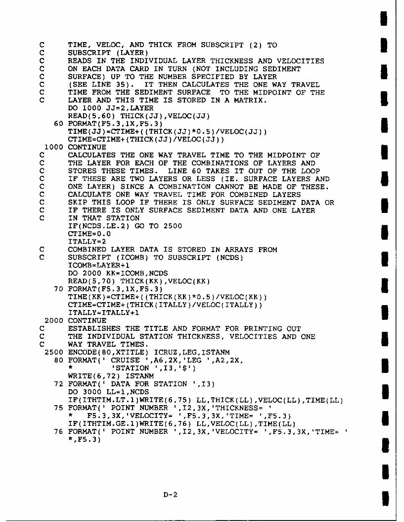
i
C TIME, VELOC, AND THICK FROM SUBSCRIPT (2) TOC SUBSCRIPT (LAYER) i
C READS IN THE INDIVIDUAL LAYER THICKNESS AND VELOCITIESC ON EACH DATA CARD IN TURN (NOT INCLUDING SEDIMENTC SURFACE) UP TO THE NUMBER SPECIFIED BY LAYERC (SEE LINE 35). IT THEN CALCULATES THE ONE WAY TRAVELC TIME FROM THE SEDIMENT SURFACE TO THE MIDPOINT OF THEC LAYER AND THIS TIME IS STORED IN A MATRIX. I
DO 1000 JJ=2,LAYERREAD(5,60) THICK(JJ),VELOC(JJ)
60 FORMAT(F5.3,1X,F5.3)TIME(JJ)=CTIME+((THICK(JJ)*0.5)/VELOC(JJ))CTIME=CTIME+(THICK(JJ)/VELOC(JJ))
1000 CONTINUEC CALCULATES THE ONE WAY TRAVEL TIME TO THE MIDPOINT OFC THE LAYER FOR EACH OF THE COMBINATIONS OF LAYERS ANDC STORES THESE TIMES. LINE 60 TAKES IT OUT OF THE LOOPC IF THESE ARE TWO LAYERS OR LESS (IE. SURFACE LAYERS AND 5C ONE LAYER) SINCE A COMBINATION CANNOT BE MADE OF THESE.C CALCULATE ONE WAY TRAVEL TIME FOR COMBINED LAYERSC SKIP THIS LOOP IF THERE IS ONLY SURFACE SEDIMENT DATA ORC IF THERE IS ONLY SURFACE SEDIMENT DATA AND ONE LAYERC IN THAT STATION
IF(NCDS.LE.2) GO TO 2500CTIME=0.0ITALLY=2
C COMBINED LAYER DATA IS STORED IN ARRAYS FROMC SUBSCRIPT (ICOMB) TO SUBSCRIPT (NCDS)
ICOMB=LAYER+ 1DO 2000 KK=ICOMB,NCDSREAD(5,70) THICK(KK),VELOC(KK)
70 FORMAT(F5.3,1X,F5.3)TIME(KK)=CTIME+((THICK(KK)*0.5)/VELOC(KK))CTIME=CTIME+(THICK(ITALLY)/VELOC(ITALLY))
ITALLY=ITALLY+l2000 CONTINUE
C ESTABLISHES THE TITLE AND FORMAT FOR PRINTING OUTC THE INDIVIDUAL STATION THICKNESS, VELOCITIES AND ONEC WAY TRAVEL TIMES.
2500 ENCODE(80,XTITLE) ICRUZ,LEG,ISTANM80 FORMAT(' CRUISE ',A6,2X,'LEG ',A2,2X,
* 'STATION ',13,'$') IWRITE(6,72) ISTANM
72 FORMAT(' DATA FOR STATION ',13)DO 3000 LL=1,NCDS iIF(ITHTIM.LT.1)WRITE(6,75) LL,THICK(LL),VELOC(LL),TIME(LL)
75 FORMAT(' POINT NUMBER ',12,3X,'THICKNESS= '* F5.3,3X,'VELOCITY= ',F5.3,3X,'TIME= ',F5.3)IF(ITHTIM.GE.1)WRITE(6,76) LL,VELOC(LL),TIME(LL)
76 FORMAT(' POINT NUMBER ',12,3X,'VELOCITY= ',F5.3,3X,'TIME=*,F5.3)
ID- 2 1
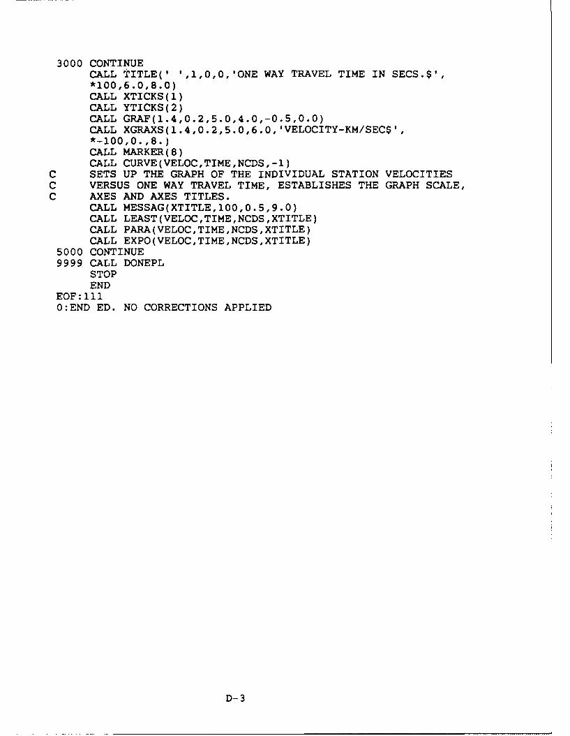
3000 CONTINUECALL TITLE(' ',1,0,0,'ONE WAY TRAVEL TIME IN SECS.$',"*100,6.0,8.0)CALL XTICKS(1)CALL YTICKS(2)CALL GRAF(1.4,0.2,5.0,4.0,-0.5,0.0)CALL XGRAXS(1.4,0.2,5.0,6.0,'VELOCITY-KM/SEC$',*-100,0.,8.)CALL MARKER(8)CALL CURVE(VELOC,TIME,NCDS,-1)
C SETS UP THE GRAPH OF THE INDIVIDUAL STATION VELOCITIESC VERSUS ONE WAY TRAVEL TIME, ESTABLISHES THE GRAPH SCALE,C AXES AND AXES TITLES.
CALL MESSAG(XTITLE,100,0.5,9.0)CALL LEAST(VELOC,TIME,NCDS,XTITLE)CALL PARA(VELOC,TIME,NCDS,XTITLE)CALL EXPO(VELOC,TIME,NCDS,XTITLE)
5000 CONTINUE9999 CALL DONEPL
STOPEND
EOF:III0:END ED. NO CORRECTIONS APPLIED
D-3

i
C SUBPROGRAM FOR LINEAR FIT OF VEL/TIME DATAC SUMX=SUM OF THE XS (VELOC)C SUMY=SUM OF THE YS (TIME)C SUMW=SUM OF THE WSC SUMXW=SUM OF THE X * W mC SUMYW=SUM OF THE Y *WC SUMXYW=SUM OF THE X*Y*W'SC SUMYSW=SUM OF Y SQ * W 3C YAVE=AVERAGE OF THE YS
SUBROUTINE LEAST(VELOC,TIME,NCDS,XTITLE)C THIS ESTABLISHES MATRICES FOR STORING VARIOUS QUANTITIESC TO BE MANIPULATED IN THE PROGRAM.
DIMENSION VELOC(12),* XEST(12),• TIME(12)CHARACTER XTITLE*36,YTITLE*37,ZTITLE*31DIMENSION X(80),
Y(80),
• W(12)C THIS SEQUENCE SETS ALL OF THE QUANTITIES TO BEC CALCULATED TO INITIAL ZERC VALUE.
SUMW=0SUMX=0SUMXW= 0SUMY=0SUMYW=0SUMXYW=0SUMYSW=0 iSUMYS=0
C WEIGHT FIRST POINT BY GIVING W(1) A HIGH VALUEC IN ORDER TO GIVE MORE WEIGHT TO THE SEDIMENT SURFACEC VELOCITY AND FORCE THE CURVE THROUGH THIS POINT, A IC WEIGHTING FACTOR IS USED IN THE CALCULATIONS AND THEC SEDIMENT SURFACE VELOCITY IS GIVEN A WEIGHT OF 5 ANDC ALL OTHER VELOCITY POINTS A WEIGHT OF ONE.
W(1)=5DO 500 LL=2,NCDS
500 W(LL)=I.C READ THROUGH VELOC AND TIME TO OBTAINC VARIABLES FOR LEAST SQUARES EQUATIONC THIS SERIES OF STATEMENTS CALCULATES THE VARIOUSC QUANTITIES (SUMS) NEEDED TO PERFORM A MATHEMATICAL IC LEAST SQUARES FIT TO THE DATA. THE DATA ARE PULLED FROMC THE MAIN PROGRAM AND NEED NOT BE READ IN AGAIN.
DO 1000 JJ=1,NCDSSUMX=SUMX+VELOC(JJ)SUMY=SUMY+TIME(JJ)SUMW=SUMW+W(JJ)SUMXW=SUMXW+(VELOC(JJ)*W(JJ))SUMYW=SUMYW+(TIME(JJ)*W(JJ))SUMXYW=SUMXYW+(VELOC(JJ)*TIME(JJ)*W(JJ))SUMYS=SUMYS+TIME(JJ)**2
ID-4 3

1000 SUMYSW=SUMYSW+(TIME(JJ)**2*W(JJ))XAVE=SUMX/NCDS
C CREATE AO VARIABLE FOR LEAST SQ EQUATIONC CALCULATES THE CONSTANTS A IN THE LINE Y=A+BX
BO=((SUMXW*SUMYSW)-(SUMYW*SUMXYW))/* ((SUMW*SUMYSW)-SUMYW**2)
C CREATE Al VARIABLE FOR LEAST SQ EQUATIONC CALCULATES THE CONSTANT B IN THE LINE Y=A+BX
B1=((SUMW*SUMXYW)-(SUMXW*SUMYW))/* ((SUMW*SUMYSW)-SUMYW**2)
C THIS SERIES OF STATEMENTS USES THE EQUATION DETERMINEDC ABOVE, Y=A+BX OR ACTUALLY X=A+BY TO DERIVE THE LINEC WHICH BEST FITS THE DATA. INCREMENTAL VALUES OF Y AREC USED ALONG WITH THE DETERMINED CONSTANTS A AND B. DERIVEC X AND Y POINTS FOR LINE BY USING EQUATION FOR EVERY TICKC MARK ON THE X AXIS
YORIG=0.0DO 2000 II=1,50Y(II)=YORIGYORIG=YORIG+0.05X(II)=BO+Bl*Y(II)
2000 CONTINUEC DETERMINES THE COEFFICIENT OF CORRELATION FOR THE LEASTC SQUARES FIT LINE AND PRINTS IT OUT.C FIND ESTIMATED YS BY USING FORMULA ON EACHC ACTUAL X VALUE
SSR=0SST=0DO 1500 LL=1,NCDSXEST(LL)=BO+(BI*TIME(LL))SSR=SSR+(VELOC(LL)-XEST(LL))**2SST=SST+(VELOC(LL)-XAVE)**2
1500 CONTINUECOC=SQRT(1-(SSR/SST))ENCODE(70,ZTITLE) COC
70 FORMAT(' CORRELATION COEFFICIENT= ',F5.3)C POINTS OUT THE COEFFICIENTS A AND B.
ENCODE(80,YTITLE) B1,BO80 FORMAT(' B1=',F6.3,2X,'BO=',F6.3,5X,'X=BO + B1*Y')
C THESE PLOT THE DATA AND THE BEST FIT LINE WITH HEADINGSC AND AXIS NOTATION.
CALL CURVE(X,Y,50,0)CALL MESSAG(YTITLE,37,0.5,-0.5)CALL MESSAG(ZTITLE,31,0.5,0.0)RETURNEND
D- 5
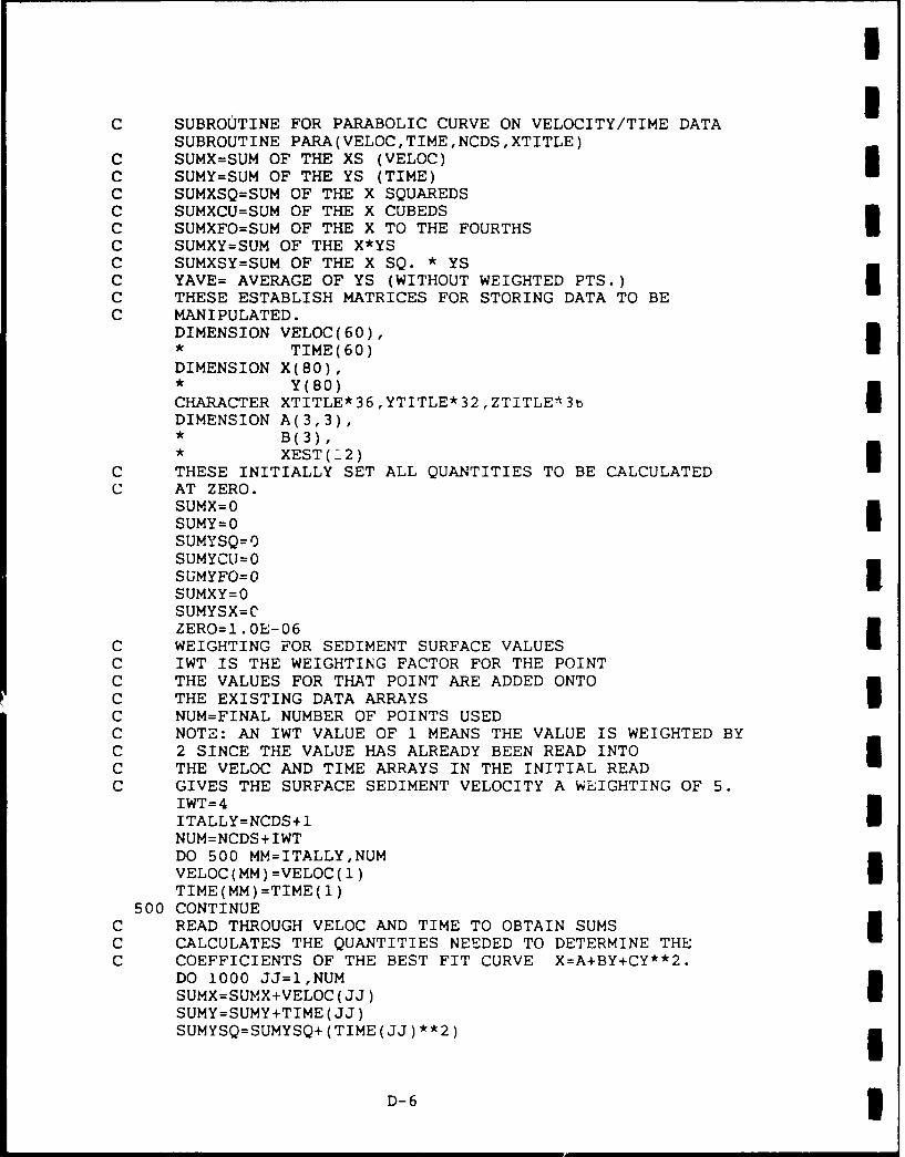
iI
C SUBROUTINE FOR PARABOLIC CURVE ON VELOCITY/TIME DATASUBROUTINE PARA(VELOC,TIME,NCDS,XTITLE)
C SUMX=SUM OF THE XS (VELOC)C SUMY=SUM OF THE YS (TIME)C SUMXSQ=SUM OF THE X SQUAREDSC SUMXCU=SUM OF THE X CUBEDSC SUMXFO=SUM OF THE X TO THE FOURTHSC SUMXY=SUM OF THE X*YSC SUMXSY=SUM OF THE X SQ. * YSC YAVE= AVERAGE OF YS (WITHOUT WEIGHTED PTS.) iC THESE ESTABLISH MATRICES FOR STORING DATA TO BEC MANIPULATED.
DIMENSION VELOC(60),• TIME(60)DIMENSION X(80),• Y(80)
CHARACTER XTITLE*36,YTITLE*32,ZTITLE*3bDIMENSION A(3,3),• B(3),• XEST(-2)
C THESE INITIALLY SET ALL QUANTITIES TO BE CALCULATEDC AT ZERO.
SUMX=0SUMY=OSUMYSQ=0SUMYCU=0SUMYFO=0 ISUMXY=0SUMYSX=CZERO=1.OE-06
C WEIGHTING FOR SEDIMENT SURFACE VALUESC IWT IS THE WEIGHTING FACTOR FOR THE POINTC THE VALUES FOR THAT POINT ARE ADDED ONTOC THE EXISTING DATA ARRAYS IC NUM=FINAL NUMBER OF POINTS USEDC NOTE: AN IWT VALUE OF 1 MEANS THE VALUE IS WEIGHTED BYC 2 SINCE THE VALUE HAS ALREADY BEEN READ INTO 5C THE VELOC AND TIME ARRAYS IN THE INITIAL READC GIVES THE SURFACE SEDIMENT VELOCITY A WEIGHTING OF 5.
IWT=4ITALLY=NCDS+INUM=NCDS+IWTDO 500 MM=ITALLY,NUMVELOC(MM)=VELOC(1) iTIME(MM)=TIME(1)
500 CONTINUEC READ THROUGH VELOC AND TIME TO OBTAIN SUMS i
C CALCULATES THE QUANTITIES NEEDED TO DETERMINE THEC COEFFICIENTS OF THE BEST FIT CURVE X=A+BY+CY**2.
DO 1000 JJ=1,NUMSUMX=SUMX+VELOC(JJ)SUMY=SUMY+TIME(JJ)SUMYSQ=SUMYSQ+(TIME(JJ)**2) 5
D-6 3
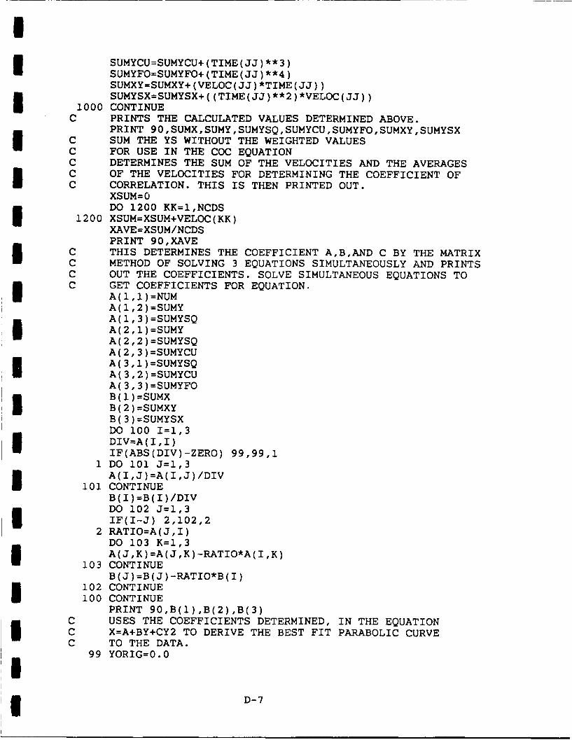
ISUMYCU=SUMYCU+(TIME(JJ)**3)SUMYFO=SUMYFO+(TIME(JJ)**4)SUMXY=SUMXY+(VELOC(JJ)*TIME(JJ))SUMYSX=SUMYSX+((TIME(JJ)**2)*VELOC(JJ))
1000 CONTINUEC PRINTS THE CALCULATED VALUES DETERMINED ABOVE.
PRINT 90,SUMX,SUMY,SUMYSQ,SUMYCU,SUMYFO,SUMXY,SUMYSXC SUM THE YS WITHOUT THE WEIGHTED VALUESC FOR USE IN THE COC EQUATIONC DETERMINES THE SUM OF THE VELOCITIES AND THE AVERAGESC OF THE VELOCITIES FOR DETERMINING THE COEFFICIENT OFC CORRELATION. THIS IS THEN PRINTED OUT.
XSUM=0DO 1200 KK=I,NCDS
1200 XSUM=XSUM+VELOC(KK)XAVE=XSUM/NCDSPRINT 90,XAVE
C THIS DETERMINES THE COEFFICIENT A,B,AND C BY THE MATRIXC METHOD OF SOLVING 3 EQUATIONS SIMULTANEOUSLY AND PRINTSC OUT THE COEFFICIENTS. SOLVE SIMULTANEOUS EQUATIONS TOC GET COEFFICIENTS FOR EQUATION.
A(1,1)=NUMA(1,2)=SUMYA(1,3)=SUMYSQA(2,1)=SUMYA(2,2)=SUMYSQA(2,3)=SUMYCU3 A(3,1)=SUMYSQA(3,2)=SUMYCUA(3,3)=SUMYFOB(1)=SUMXB(2)=SUMXYB(3)=SUMYSX
DO 100 I=1,3DIV=A(I,I)IF(ABS(DIV)-ZERO) 99,99,1
1 DO 101 J=1,3A(I,J)=A(I,J)/DIV
101 CONTINUEB(I)=B(I)/DIVDO 102 J=1,3IF(I-J) 2,102,2
2 RATIO=A(J,I)DO 103 K=1,3A(J,K)=A(J,K)-RATIO*A(I,K)
103 CONTINUEB(J)=B(J)-RATIO*B(I)
102 CONTINUE100 CONTINUE
PRINT 90,B(1),B(2),B(3)C USES THE COEFFICIENTS DETERMINED, IN THE EQUATIONSC X=A+BY+CY2 TO DERIVE THE BEST FIT PARABOLIC CURVEC TO THE DATA.
99 YORIG=0.0
I5 D-7
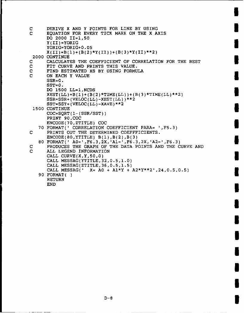
U
C DERIVE X AND Y POINTS FOR LINE BY USING 3C EQUATION FOR EVERY TICK MARK ON THE X AXIS
DO 2000 II=1,50Y(II)=YORIG 3YORIG=YORIG+0.05X(II)=B(1)+(B(2)*Y(II))+(B(3)*Y(II)**2)
2000 CONTINUEC CALCULATES THE COEFFICIENT OF CORRELATION FOR THE BESTC FIT CURVE AND PRINTS THIS VALUE.C FIND ESTIMATED XS BY USING FORMULAC ON EACH Y VALUE 5
SSR=0.SST=0.DO 1500 LL=1,NCDSXEST(LL)=B(1)+(B(2)*TIME(LL))+(B(3)*TIME(LL)**2)SSR=SSR+(VELOC(LL)-XEST(LL))**2SST=SST+(VELOC(LL)-XAVE)**2
1500 CONTINUECOC=SQRT(1-(SSR/SST))PRINT 90,COCENCODE(70,ZTITLE) COC
70 FORMAT(' CORRELATION COEFFICIENT PARA= ',F5.3)C PRINTS OUT THE DETERMINED COEFFFICIENTS.
ENCODE(80,YTITLE) B(1),B(2),B(3)80 FORMAT(' AO=',F6.3,2X,'AI=',F6.3,2X,'A2=',F6.3)
C PRODUCES THE GRAPH OF THE DATA POINTS AND THE CURVE ANDC ALL LEGEND INFORMATION
CALL CURVE(X,Y,50,0) UCALL MESSAG(YTITLE,32,0.5,1.0)CALL MESSAG(ZTITLE,36,0.5,1.5)CALL MESSAG(' X= AO + AI*Y + A2*Y**2',24,0.5,0.5)
90 FORMAT( )RETURNEND 3
IIIIII
D- 8 3
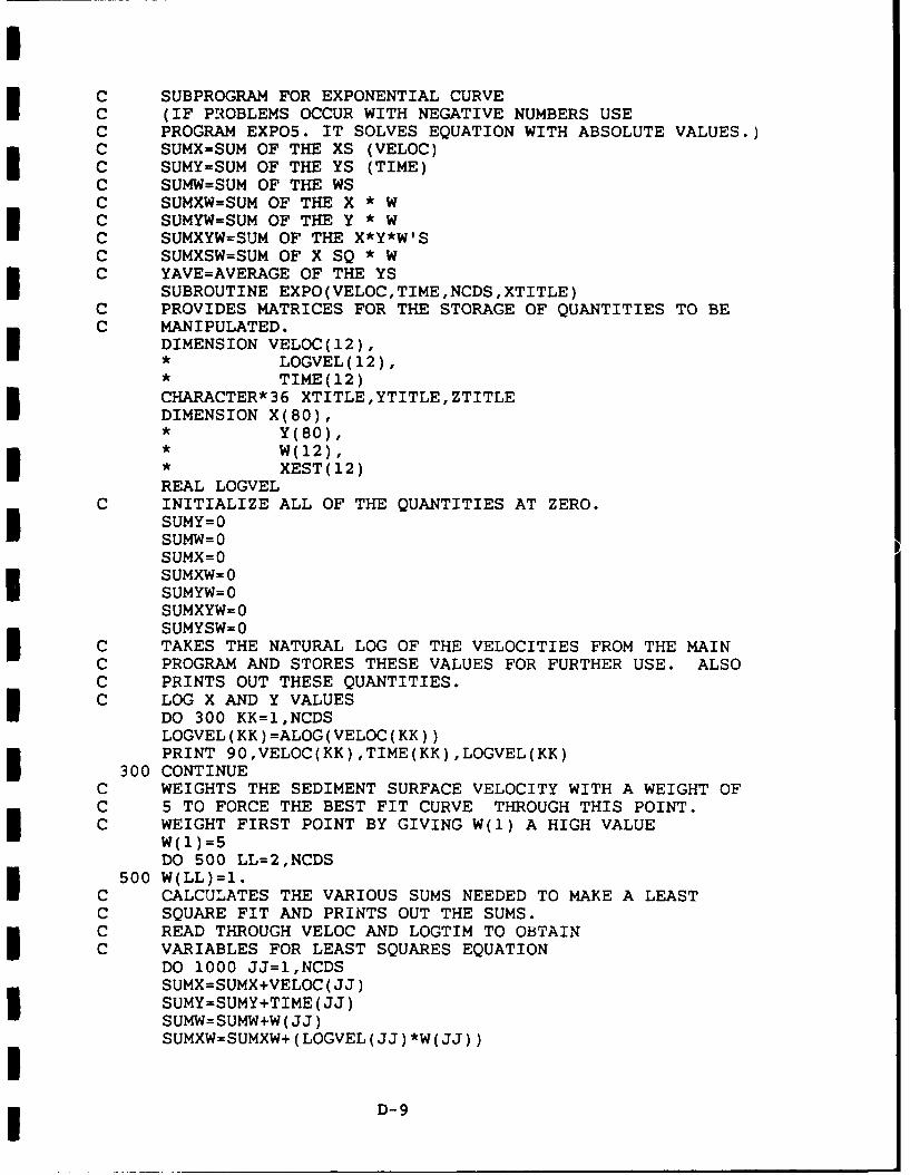
II
C SUBPROGRAM FOR EXPONENTIAL CURVEC (IF PROBLEMS OCCUR WITH NEGATIVE NUMBERS USEC PROGRAM EXPO5. IT SOLVES EQUATION WITH ABSOLUTE VALUES.)C SUMX=SUM OF THE XS (VELOC)C SUMY=SUM OF THE YS (TIME)C SUMW=SUM OF THE WS
C SUMXW=SUM OF THE X * WC SUMYW=SUM OF THE Y * WC SUMXYW=SUM OF THE X*Y*W'SC SUMXSW=SUM OF X SQ * wC YAVE=AVERAGE OF THE YS
SUBROUTINE EXPO(VELOC,TIME,NCDS,XTITLE)C PROVIDES MATRICES FOR THE STORAGE OF QUANTITIES TO BEC MANIPULATED.
DIMENSION VELOC(12),• LOGVEL(12),* TIME(12)
CHARACTER*36 XTITLE,YTITLE,ZTITLEDIMENSION X(80),• Y(80),S* W(12),
• XEST(12)REAL LOGVEL
C INITIALIZE ALL OF THE QUANTITIES AT ZERO.SUMY=0SUMW=ISUMX=0SUMXW=0
SUMYW=0SUMXYW=0SUMYSW=0
C TAKES THE NATURAL LOG OF THE VELOCITIES FROM THE MAINC PROGRAM AND STORES THESE VALUES FOR FURTHER USE. ALSOC PRINTS OUT THESE QUANTITIES.C LOG X AND Y VALUES
DO 300 KK=1,NCDSLOGVEL(KK)=ALOG(VELOC(KK))PRINT 90,VELOC(KK),TIME(KK),LOGVEL(KK)
300 CONTINUEC WEIGHTS THE SEDIMENT SURFACE VELOCITY WITH A WEIGHT OFC 5 TO FORCE THE BEST FIT CURVE THROUGH THIS POINT.C WEIGHT FIRST POINT BY GIVING W(l) A HIGH VALUE
W(1)=WDO 500 LL=2,NCDS
500 W(LL)=I.C CALCULATES THE VARIOUS SUMS NEEDED TO MAKE A LEASTC SQUARE FIT AND PRINTS OUT THE SUMS.C READ THROUGH VELOC AND LOGTIM TO OBTAINC VARIABLES FOR LEAST SQUARES EQUATION
DO 1000 JJ=1,NCDSSUMX=SUMX+VELOC(JJ)SUMY=SUMY+TIME(JJ)SUMW=SUMW+W(JJ)SUMXW=SUMXW+(LOGVEL(JJ)*W(JJ))
D-9
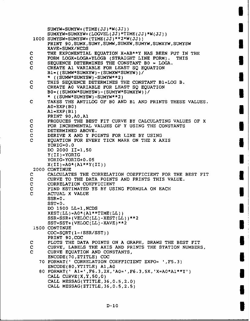
I
SUMYW=SUMYW+(TIME(JJ)*W(JJ)) 3SUMXYW=SUMXYW+(LOGVEL(JJ)*TIME(JJ)*W(JJ))
1000 SUMYSW=SUMYSW+(TIME(JJ)**2*W(JJ))PRINT 90,SUMX,SUMY,SUMW,SUMXW,SUMYW,SUMXYW,SUMYSW 3XAVE=SUMX/NCDS
C THE EXPONENTIAL EQUATION X=AB**Y HAS BEEN PUT IN THEC FORM LOGX=LOGA+YLOGB (STRAIGHT LINE FORM). THISC SEQUENCE DETERMINES THE CONSTANT BO = LOGA.C CREATE Al VARIABLE FOR LEAST SQ EQUATION
Bl=((SUMW*SUMXYW)-(SUMXW*SUMYW))/ I* ((SUMW*SUMYSW)-SUMYW**2)
C THIS SEQUENCE DETERMINES THE CONSTANT B1=LOG B.C CREATE AO VARIABLE FOR LEAST SQ EQUATION
BO=((SUMXW*SUMYSW)-(SUMYW*SUMXYW))/ 3* ((SUMW*SUMYSW)-SUMYW**2)
C TAKES THE ANTILOG OF BO AND B1 AND PRINTS THESE VALUES.AO=EXP(BO)A1=EXP(BI)PRINT 90,AO,AI
C PRODUCES THE BEST FIT CURVE BY CALCULATING VALUES OF XC FOR INCREMENTAL VALUES OF Y USING THE CONSTANTSC DETERMINED ABOVE.C DERIVE X AND Y POINTS FOR LINE BY USINGC EQUATION FOR EVERY TICK MARK ON THE X AXIS
YORIG=0.0DO 2000 II=1,50Y(II)=YORIGYORIG=YORIG+0.05X(II)=AO*(A1**Y(II))
2000 CONTINUEC CALCULATES THE CORRELATION COEFFICIENT FOR THE BEST FITC CURVE TO THE DATA POINTS AND PRINTS THIS VALUE.C CORRELATION COEFFICIENTC FIND ESTIMATED YS BY USING FORMULA ON EACHC ACTUAL X VALUE U
SSR=0.SST=0.DO 1500 LL=1,NCDSXEST(LL)=AO*(A1**TIME(LL))SSR=SSR+(VELOC(LL)-XEST(LL))**2SST=SST+(VELOC(LL)-XAVE)**2
1500 CONTINUECOC=SQRT(1-(SSR/SST))PRINT 90,COC
C PLOTS THE DATA POINTS ON A GRAPH, DRAWS THE BEST FITC CURVE, LABELS THE AXIS AND PRINTS THE STATION NUMBERS,C CURVE EQUATION AND CONSTANTS,
ENCODE(70,ZTITLE) COC 570 FORMAT(' CORRELATION COEFFICIENT EXPO= ',F5.3)
ENCODE(80,YTITLE) A1,AO80 FORMAT(' AI=',F6.3,2X,'AO=',F6.3,5X,'X=AO*AI**Y')
CALL CURVE(X,Y,50,0)CALL MESSAG(YTITLE,36,0.5,2.0)CALL MESSAG(ZTITLE,36,0.5,2.5) 5
D-10 3

90 FORMAT(CALL ENDPL(1)RETURN
* END
IIIIIIIIIIIIIII
i D-II
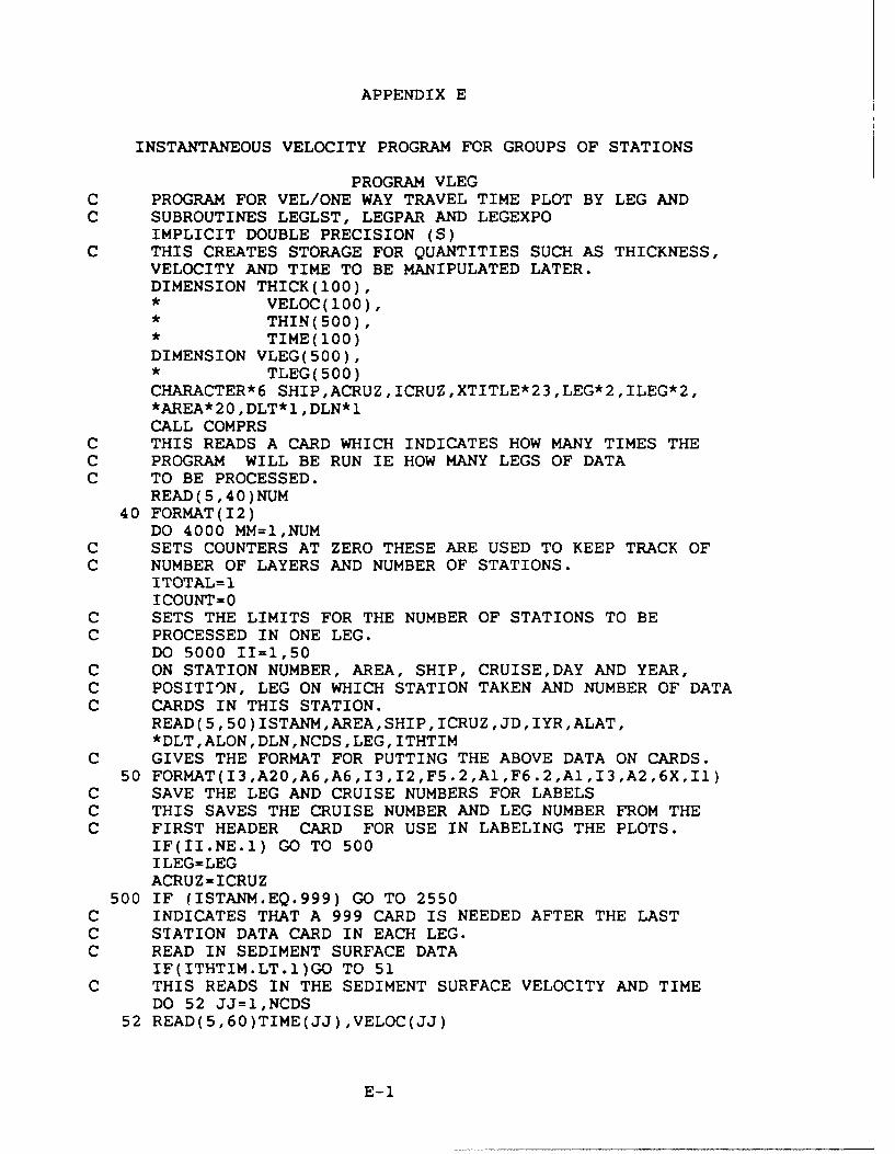
APPENDIX E
INSTANTANEOUS VELOCITY PROGRAM FOR GROUPS OF STATIONS
PROGRAM VLEGC PROGRAM FOR VEL/ONE WAY TRAVEL TIME PLOT BY LEG ANDC SUBROUTINES LEGLST, LEGPAR AND LEGEXPO
IMPLICIT DOUBLE PRECISION (S)C THIS CREATES STORAGE FOR QUANTITIES SUCH AS THICKNESS,
VELOCITY AND TIME TO BE MANIPULATED LATER.DIMENSION THICK(100),
VELOC(100),THIN(500),TIME(100)
DIMENSION VLEG(500),TLEG(500)
CHARACTER*6 SHIPACRUZICRUZXTITLE*23,LEG*2,ILEG*2,*AREA*20,DLT*1,DLN*lCALL COMPRS
C THIS READS A CARD WHICH INDICATES HOW MANY TIMES THEC PROGRAM WILL BE RUN IE HOW MANY LEGS OF DATAC TO BE PROCESSED.
READ(5,40)NUM40 FORMAT(I2)
DO 4000 MM=1,NUMC SETS COUNTERS AT ZERO THESE ARE USED TO KEEP TRACK OFC NUMBER OF LAYERS AND NUMBER OF STATIONS.
ITOTAL=lICOUNT=O
C SETS THE LIMITS FOR THE NUMBER OF STATIONS TO BEC PROCESSED IN ONE LEG.
DO 5000 II=1,50C ON STATION NUMBER, AREA, SHIP, CRUISEDAY AND YEAR,C POSITION, LEG ON WHICH STATION TAKEN AND NUMBER OF DATAC CARDS IN THIS STATION.
READ(5,50)ISTANMAREASHIPICRUZJDIYRALAT,*DLTALONDLNNCDSLEGITHTIM
C GIVES THE FORMAT FOR PUTTING THE ABOVE DATA ON CARDS.50 FORMAT(I3,A20,A6,A6,I3,I2,F5.2,AlF6.2,AlI3,A2,6XIl)
C SAVE THE LEG AND CRUISE NUMBERS FOR LABELSC THIS SAVES THE CRUISE NUMBER AND LEG NUMBER FROM THEC FIRST HEADER CARD FOR USE IN LABELING THE PLOTS.
IF(II.NE.1) GO TO 500ILEG=LEGACRUZ=ICRUZ
500 IF (ISTANM.EQ.999) GO TO 2550C INDICATES THAT A 999 CARD IS NEEDED AFTER THE LASTC STATION DATA CARD IN EACH LEG.C READ IN SEDIMENT SURFACE DATA
IF(ITHTIM.LT.1)GO TO 51C THIS READS IN THE SEDIMENT SURFACE VELOCITY AND TIME
DO 52 JJ=1,NCDS52 READ(5,60)TIME(JJ),VELOC(JJ)
E-1
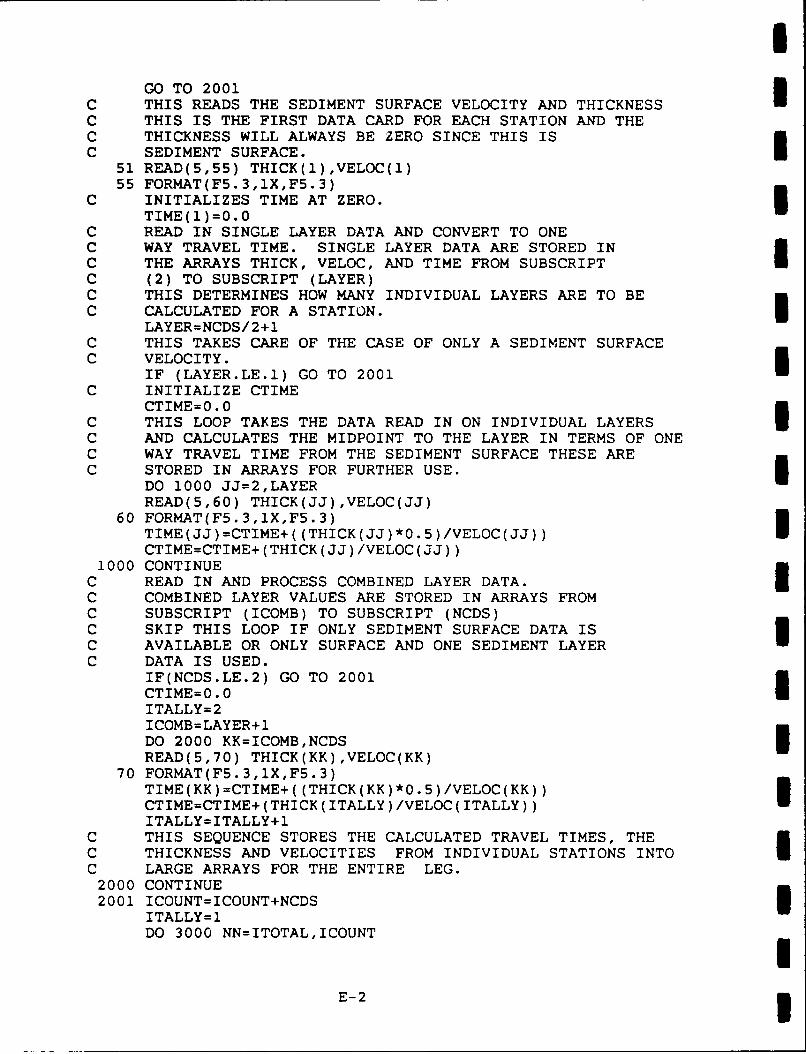
I
GO TO 2001C THIS READS THE SEDIMENT SURFACE VELOCITY AND THICKNESSC THIS IS THE FIRST DATA CARD FOR EACH STATION AND THEC THICKNESS WILL ALWAYS BE ZERO SINCE THIS ISC SEDIMENT SURFACE. I
51 READ(5,55) THICK(1),VELOC(1)55 FORMAT(F5.3,1X,F5.3)
C INITIALIZES TIME AT ZERO.TIME(1)=0.0
C READ IN SINGLE LAYER DATA AND CONVERT TO ONEC WAY TRAVEL TIME. SINGLE LAYER DATA ARE STORED INC THE ARRAYS THICK, VELOC, AND TIME FROM SUBSCRIPT IC (2) TO SUBSCRIPT (LAYER)C THIS DETERMINES HOW MANY INDIVIDUAL LAYERS ARE TO BEC CALCULATED FOR A STATION. I
LAYER=NCDS/2+1C THIS TAKES CARE OF THE CASE OF ONLY A SEDIMENT SURFACEC VELOCITY.
IF (LAYER.LE.1) GO TO 2001C INITIALIZE CTIME
CTIME=0.0C THIS LOOP TAKES THE DATA READ IN ON INDIVIDUAL LAYERSC AND CALCULATES THE MIDPOINT TO THE LAYER IN TERMS OF ONEC WAY TRAVEL TIME FROM THE SEDIMENT SURFACE THESE AREC STORED IN ARRAYS FOR FURTHER USE. 5
DO 1000 JJ=2,LAYERREAD(5,60) THICK(JJ),VELOC(JJ)
60 FORMAT(F5.3,1X,F5.3)TIME(JJ)=CTIME+((THICK(JJ)*0.5)/VELOC(JJ))CTIME=CTIME+(THICK(JJ)/VELOC(JJ))
1000 CONTINUEC READ IN AND PROCESS COMBINED LAYER DATA.C COMBINED LAYER VALUES ARE STORED IN ARRAYS FROMC SUBSCRIPT (ICOMB) TO SUBSCRIPT (NCDS)C SKIP THIS LOOP IF ONLY SEDIMENT SURFACE DATA IS 3C AVAILABLE OR ONLY SURFACE AND ONE SEDIMENT LAYERC DATA IS USED.
IF(NCDS.LE.2) GO TO 2001CTIME=0.0ITALLY=2ICOMB=LAYER+IDO 2000 KK=ICOMB,NCDSREAD(5,70) THICK(KK),VELOC(KK)
70 FORMAT(F5.3,1XF5.3)TIME(KK)=CTIME+((THICK(KK)*0.5)/VELOC(KK))CTIME=CTIME+(THICK(ITALLY)/VELOC(ITALLY))ITALLY=ITALLY+I
C THIS SEQUENCE STORES THE CALCULATED TRAVEL TIMES, THEC THICKNESS AND VELOCITIES FROM INDIVIDUAL STATIONS INTOC LARGE ARRAYS FOR THE ENTIRE LEG.
2000 CONTINUE2001 ICOUNT=ICOUNT+NCDS I
ITALLY=1DO 3000 NN=ITOTAL,ICOUNT
E-2 3
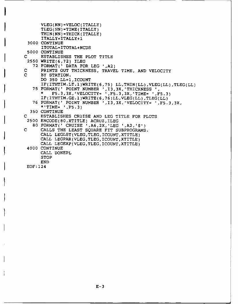
IVLEG(NN)=VELOC(ITALLY)TLEG(IIN)=TIME(ITALLY)THIN(NN)=THICK(ITALLY)ITALLY=ITALLY+1
3000 CONTINUEITOTAL=ITOTAL+NCDS
5000 CONTINUEC ESTABLISHES THE PLOT TITLE
2550 WRITE(6,72) ILEG72 FORMAT(' DATA FOR LEG ',A2)
C PRINTS OUT THICKNESS, TRAVEL TIME, AND VELOCITYC BY STATION.
DO 350 LL=1,ICOUNTIF(ITHTIM.LT.1)WRITE(6,75) LL,THIN(LL),VLEG(LL),TLEG(LL)
75 FORMAT(' POINT NUMBER ',13,3X,'THICKNESS ',F5.3,3X,'VELOCITY= ',F5.3,3X,'TIME= ',F5.3)
IF(ITHTIM.GE.1)WRITE(6,76)LL,VLEG(LL),TLEG(LL)76 FORMAT(' POINT NUMBER ',13,3X,'VELOCITY= ',F5.3,3X,
*'TIME= ',F5.3)350 CONTINUE
C ESTABLISHES CRUISE AND LEG TITLE FOR PLOTS2500 ENCODE(80,XTITLE) ACRUZ,ILEG
80 FORMAT(' CRUISE ',A6,2X,'LEG ',A2,'$')C CALLS THE LEAST SQUARE FIT SUBPROGRAMS.
CALL LEGLST(VLEG,TLEG,ICOUNT,XTITLE)CALL LEGPAR(VLEG,TLEG,ICOUNT,XTITLE)CALL LEGEXP(VLEG,TLEG,ICOUNT,XTITLE)
4000 CONTINUECALL DONEPLSTOPEND
EOF:124
E-3
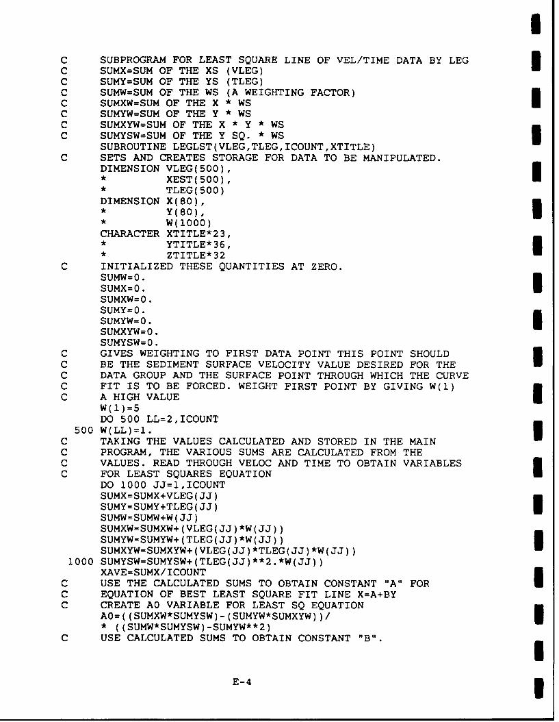
IC SUBPROGRAM FOR LEAST SQUARE LINE OF VEL/TIME DATA BY LEGC SUMX=SUM OF THE XS (VLEG)IC SUMY=SUM OF THE YS (TLEG)
C SUMW=SUM OF THE WS (A WEIGHTING FACTOR)C SUMXW=SUM OF THE X * WSC SUMYW=SUM OF THE Y * WSC SUMXYW=SUM OF THE X * Y * WSC SUMYSW=SUM OF THE Y SQ. * WS 3
SUBROUTINE LEGLST(VLEG,TLEG,ICOUNT,XTITLE)C SETS AND CREATES STORAGE FOR DATA TO BE MANIPULATED.
DIMENSION VLEG(500),• XEST(500),• TLEG(500)
DIMENSION X(80),* ~Y(80),I
• W(1000)
CHARACTER XTITLE*23,YTITLE*36,
• ZTITLE*32C INITIALIZED THESE QUANTITIES AT ZERO.
SUMW=0.SUMX=0.SUMXW=0.SUMY=O.SUMYW=O.SUMXYW=0.SUMYSW=0.
C GIVES WEIGHTING TO FIRST DATA POINT THIS POINT SHOULDC BE THE SEDIMENT SURFACE VELOCITY VALUE DESIRED FOR THEC DATA GROUP AND THE SURFACE POINT THROUGH WHICH THE CURVEC FIT IS TO BE FORCED. WEIGHT FIRST POINT BY GIVING W(1)C A HIGH VALUE I
W(1)=5DO 500 LL=2,ICOUNT
500 W(LL)=I. 3C TAKING THE VALUES CALCULATED AND STORED IN THE MAINC PROGRAM, THE VARIOUS SUMS ARE CALCULATED FROM THEC VALUES. READ THROUGH VELOC AND TIME TO OBTAIN VARIABLESC FOR LEAST SQUARES EQUATION
DO 1000 JJ=1,ICOUNTSUMX=SUMX+VLEG(JJ)SUMY=SUMY+TLEG(JJ)SUMW=SUMW+W(JJ)SUMXW=SUMXW+(VLEG(JJ)*W(JJ))SUMYW=SUMYW+(TLEG(JJ)*W(JJ))SUMXYW=SUMXYW+(VLEG(JJ)*TLEG(JJ)*W(JJ))
1000 SUMYSW=SUMYSW+(TLEG(JJ)**2.*W(JJ))XAVE=SUMX/ICOUNT
C USE THE CALCULATED SUMS TO OBTAIN CONSTANT "A" FORC EQUATION OF BEST LEAST SQUARE FIT LINE X=A+BYC CREATE AO VARIABLE FOR LEAST SQ EQUATION
AO=((SUMXW*SUMYSW)-(SUMYW*SUMXYW))/* ((SUMW*SUMYSW)-SUMYW**2)
C USE CALCULATED SUMS TO OBTAIN CONSTANT "B".
E-4 3
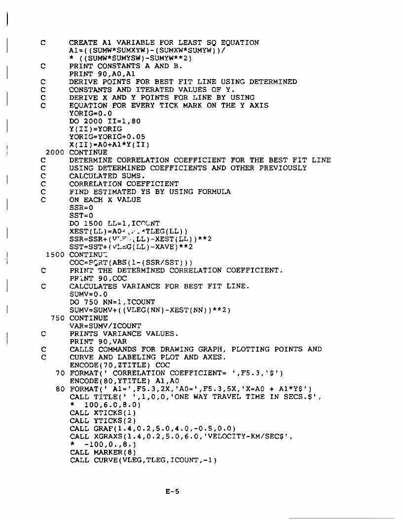
C CREATE Al VARIABLE FOR LEAST SQ EQUATIONAl=((SUMW*SUMXYW)-(SUMXW*SUMYW))/* ((SUMW*SUMYSW)-SUMYW**2)
C PRINT CONSTANTS A AND B.PRINT 90,AO,Al
C DERIVE POINTS FOR BEST FIT LINE USING DETERMINEDC CONSTANTS AND ITERATED VALUES OF Y.C DERIVE X AND Y POINTS FOR LINE BY USINGC EQUATION FOR EVERY TICK MARK ON THE Y AXIS
YORIG=0.0DO 2000 II=1,80Y(II)=YORIGYORIG=YORIG+0.05X(II)=AO+Al*Y(II)
2000 CONTINUEC DETERMINE CORRELATION COEFFICIENT FOR THE BEST FIT LINEC USING DETERMINED COEFFICIENTS AND OTHER PREVIOUSLYC CALCULATED SUMS.C CORRELATION COEFFICIENTC FIND ESTIMATED YS BY USING FORMULAC ON EACH X VALUE
SSR=0SST=0DO 1500 LL=1,IC(ThNTXEST(LL)=A0J, ,--TLEG(LL))SSR=SSR+(VL'F-(LL)-XEST(LL))**2SST=SST+(VLrG(LL)-XAVE)**2
1500 CONTINU•COC=SQRT(ABS(1-(SSR/SST)))
C PRINT THE DETERMINED CORRELATION COEFFICIENT.PPiNT 90,COC
C CALCULATES VARIANCE FOR BEST FIT LINE.SUMV=0.0DO 750 NN=I,ICOUNTSUMV=SUMV+((VLEG(NN)-XEST(NN))**2)
750 CONTINUEVAR=SUMV/ICOUNT
C PRINTS VARIANCE VALUES.PRINT 90,VAR
C CALLS COMMANDS FOR DRAWING GRAPH, PLOTTING POINTS ANDC CURVE AND LABELING PLOT AND AXES.
ENCODE(70,ZTITLE) COC70 FORMAT(' CORRELATION COEFFICIENT= ',F5.3,'$')
ENCODE(80,YTITLE) Al,AO80 FORMAT(' A1=',F5.3,2X,'AO=',F5.3,5X,'X=AO + Al*Y$')
CALL TITLE(' ',1,0,0,'ONE WAY TRAVEL TIME IN SECS.$'.* 100,6.0,8.0)
CALL XTICKS(1)CALL YTICKS(2)CALL GRAF(l.4,0.2,5.0,4.0,-0.5,0.0)CALL XGRAXS(1.4,0.2,5.0,6.0,'VELOCITY-KM/SEC$',* -100,0.,8.)CALL MARKER(8)CALL CURVE(VLEG,TLEG,ICOUNT,-l)
E-5
CALL CURVE(X,Y,19,0)CALL HESSAG(YTITLE, 100,0. 5,-O. 5)CALL MESSAG(XTITLE, 100,0.5,9.0)CALL MESSAG( ZTITLE, 100,0.5/0.0)
90 FORMAT(IRETURNEND
E-6

C SUBPROGRAM FOR PARABOLIC CURVE ON VEL/TIME DATA BY LEGSUBROUTINE LEGPAR(VLEG,TLEG,ICOUNT,XTITLE)
C SUMX=SUM OF THE XS (VELOC)C SUMY=SUM OF THE YS (TIME)C SUMYSQ=SUM OF THE Y SQUAREDSC SUMYCU=SUM OF THE Y CUBEDSC SUMYFO=SUM OF THE Y TO THE FOURTHSC SUMXY=SUM OF THE X*YSC SUMYSX=SUM OF THE Y SQ. * XSC XAVE= AVERAGE OF XS (WITHOUT WEIGHTED PTS.)C ESTABLISH LIMIT AND STORAGE FOR DATA TO BE MANIPULATED.
DIMENSION VLEG(500),• TLEG(500)
DIMENSION X(80),• Y(80),• A(3,3),• B(3),• WTVEL(5),• WTTIM(5),• XEST(500)
CHARACTER XTITLE*23,• YTITLE*30,• ZTITLE*32
C INITIALIZES SUMS TO ZERO.SUMX=O.SUMY=Q.SUMYSQ=O.SUMYCU=O.SUMYFO=O.SUMXY=O.SUMYSX=Q.ZERO=1.OE-06
C THIS WEIGHTS THE INITIAL DATA POINT (SEDIMENT SURFACEC VELOCITY) WITH A WEIGHT AS SPECIFIED IN LINE 276 WHILEC ALL OTHER DATA POINTS HAVE A VALUE OF ONE.C WEIGHTING FOR SPECIFIC POINTSC VALUES TO BE WEIGHTED ARE ADDED ONTO THE END OFC EXISTING DATA ARRAYS AND PROCESSED AS ACTUAL POINTSC ISED=NUMBER OF POINTS BEING WEIGHTEDC WTVEL AND WTTIM ARE ARRAYS THAT HOLD THE VALUESC THAT ARE TO BE WEIGHTEDC IWT IS AN ARRAY WHICH HOLDS THE WEIGHT FACTORC FOR THE WTVEL AND WTTIM VALUES OF THE CORRESPONDINGC SUBSCRIPT.C NOTE: AN IWT VALUE OF 1 MEANS THAT A VALUE IS BEINGC WEIGHTED BY 2 SINCE THE VALUE HAS ALREADY BEEN READC INTO VLEG AND TLEG ARRAYS ON THE INITIAL READC NUM= FINAL NUMBER OF POINTS AFTER WEIGHTING
WTTIM(1)=0.000WTVEL(1)=VLEG(1)IWT=5ITALLY=ICOUNT+INUM=ICOUNT+IWTDO 500 NN=ITALLY,NUM
E-7

I
VLEG(NN)=WTVEL(1)TLEG(NN)=WTTIM(1)
500 CONTINUEC THIS CALCULATES THE SUM OF THE VARIOUS SUMS NEEDED FORC MAKING THE LEAST SQUARE PARABOLIC FIT TO THE DATA. DATAC IS PULLED FROM THE MAIN PROGRAM.C READ THROUH VELOC AND TIME TO OBTAIN SUMS
DO 1000 JJ=1,NUM USUMX=SUMX+VLEG(JJ)SUMY=SUMY+TLEG(JJ)SUMYSQ=SUMYSQ+(TLEG(JJ) **2)SUMYCU=SUMYCU+(TLEG(JJ)**3)SUMYFO=SUMYFO+(TLEG(JJ)**4)SUMXY=SUMXY+(VLEG(JJ)*TLEG(JJ))SUMYSX=SUMYSX+((TLEG(JJ)**2)*VLEG(JJ))
1000 CONTINUEC CALCULATES THE SUM OF THE VELOCITIES FOR USE LATER INC THE COEFFICIENT OF CORRELATION COMPUTATION. iC SUM THE XS WITHOUT THE WEIGHTED VALUES TOC FIND A TRUE AVERAGE FOR THE COC EQUATION
XSUM=0.DO 1200 KK=1,ICOUNT
1200 XSUM=XSUM+VLEG(KK)XAVE=XSUM/ICOUNT
C DETERMINE COEFFICIENT OF LEAST SQUARE BEST FIT PARABOLAC CURVE X=A+BY+CY2 USING METHOD OF SIMULTANEOUS SOLUTIONC OF THREE EQUATIONS BY MATRIX METHOD . PRINT THE THREEC COEFFICIENTS. SOLVE SIMULTANEOUS EQUATIONS FORC COEFFICIENTS OF PARABOLIC EQUATION
A(1,1)=NUMA(1,2)=SUMYA(1,3)=SUMYSQA(2,1)=SUMYA(2,2)=SUMYSQA(2,3)=SUMYCUA(3,1)=SUMYSQA(3,2)=SUMYCUA(3,3)=SUMYFOB(1)=SUMXB(2)=SUMXY
B(3)=SUMYSXDO 100 I=1,3DIV=A(I,I)IF(ABS(DIV)-ZERO) 99.99,1
1 DO 101 J=1,3A(I,J)=A(I,J)/DIV
101 CONTINUEB(I)=B(I)/DIVDO 102 J=1,3IF(I-J) 2,102,2
2 RATIO=A(J,I)DO 103 K=1,3A(J,K)=A(J,K)-RATIO*A(I,K)
103 CONTINUE
E-8 1
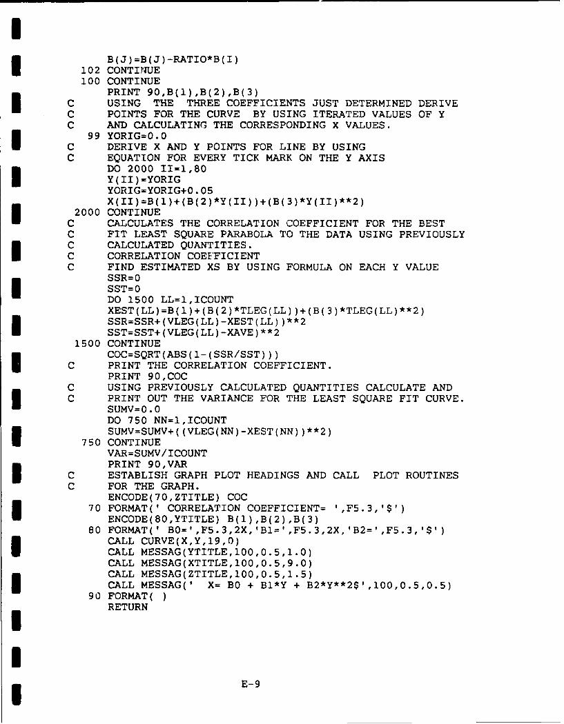
IB(J)=B(J)-RATIO*B(I)
102 CONTINUE100 CONTINUE
PRINT 90,B(1),B(2),B(3)C USING THE THREE COEFFICIENTS JUST DETERMINED DERIVEC POINTS FOR THE CURVE BY USING ITERATED VALUES OF YC AND CALCULATING THE CORRESPONDING X VALUES.
99 YORIG=0.0C DERIVE X AND Y POINTS FOR LINE BY USINGC EQUATION FOR EVERY TICK MARK ON THE Y AXIS
DO 2000 II=1,80Y(II)=YORIGYORIG=YORIG+0.05X(II)=B(1)+(B(2)*Y(II))+(B(3)*Y(II)**2)
2000 CONTINUEC CALCULATES THE CORRELATION COEFFICIENT FOR THE BESTC FIT LEAST SQUARE PARABOLA TO THE DATA USING PREVIOUSLYC CALCULATED QUANTITIES.C CORRELATION COEFFICIENTC FIND ESTIMATED XS BY USING FORMULA ON EACH Y VALUE
SSR=0SST=0DO 1500 LL=1,ICOUNTXEST(LL)=B(1)+(B(2)*TLEG(LL))+(B(3)*TLEG(LL)**2)SSR=SSR+(VLEG(LL)-XEST(LL))**2SST=SST+(VLEG(LL)-XAVE)**2
1500 CONTINUECOC=SQRT(ABS(1-(SSR/SST)))
C PRINT THE CORRELATION COEFFICIENT.PRINT 90,COC
C USING PREVIOUSLY CALCULATED QUANTITIES CALCULATE ANDC PRINT OUT THE VARIANCE FOR THE LEAST SQUARE FIT CURVE.
SUMV=0.0DO 750 NN=1,ICOUNTSUMV=SUMV+((VLEG(NN)-XEST(NN))**2)
750 CONTINUEVAR=SUMV/ICOUNT
PRINT 90,VARC ESTABLISH GRAPH PLOT HEADINGS AND CALL PLOT ROUTINESC FOR THE GRAPH.
ENCODE(70,ZTITLE) COC70 FORMAT(' CORRELATION COEFFICIENT= ',F5.3,'$')
ENCODE(80,YTITLE) B(1),B(2),B(3)80 FORMAT(' BO=',F5.3,2X,'B1=',F5.3,2X,'B2=',F5.3,'$')
CALL CURVE(X,Y,19,0)CALL MESSAG(YTITLE,100,0.5,1.0)CALL MESSAG(XTITLE,100,0.5,9.0)CALL MESSAG(ZTITLE,100,0.5,1.5)CALL MESSAG(' X= BO + B1*Y + B2*Y**2$',100,0.5,0.5)
90 FORMAT(RETURN
I* E- 9
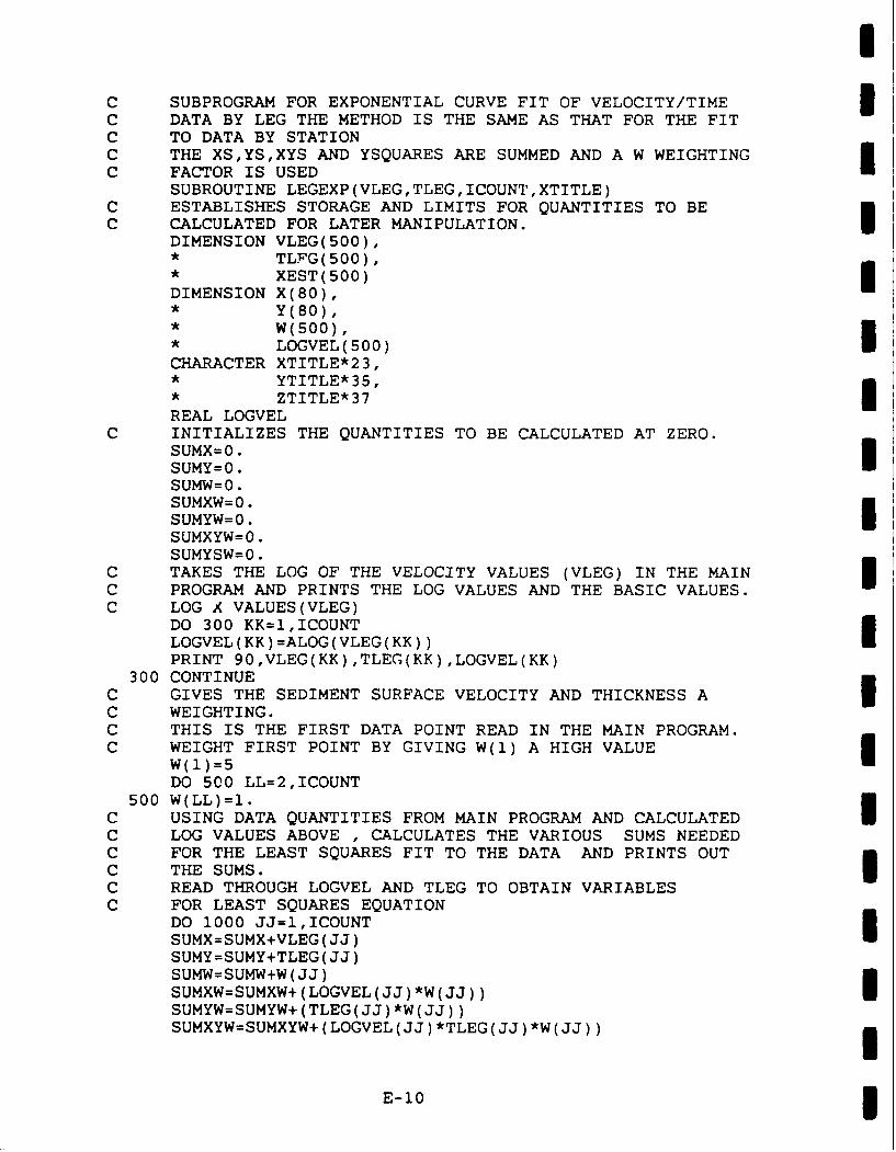
C SUBPROGRAM FOR EXPONENTIAL CURVE FIT OF VELOCITY/TIMEC DATA BY LEG THE METHOD IS THE SAME AS THAT FOR THE FITC TO DATA BY STATIONC THE XS,YS,XYS AND YSQUARES ARE SUMMED AND A W WEIGHTINGC FACTOR IS USED
SUBROUTINE LEGEXP(VLEG,TLEG,ICOUNT,XTITLE)C ESTABLISHES STORAGE AND LIMITS FOR QUANTITIES TO BEC CALCULATED FOR LATER MANIPULATION.
DIMENSION VLEG(500),* TLPG(500),
XEST(500) IDIMENSION X(80),* Y(80),* W(500),
* LOGVEL(500)CHARACTER XTITLE*23,* YTITLE*35,
, ZTITLE*37REAL LOGVEL
C INITIALIZES THE QUANTITIES TO BE CALCULATED AT ZERO.SUMX=0.SUMY=0.SUMW=0.SUMXW=0.SUMYW=O.SUMXYW=0.
SUMYSW=0.C TAKES THE LOG OF THE VELOCITY VALUES (VLEG) IN THE MAINC PROGRAM AND PRINTS THE LOG VALUES AND THE BASIC VALUES.C LOG X VALUES(VLEG)
DO 300 KK=1,ICOUNTLOGVEL(KK)=ALOG(VLEG(KK))PRINT 90,VLEG(KK),TLEG(KK),LOGVEL(KK)
300 CONTINUEC GIVES THE SEDIMENT SURFACE VELOCITY AND THICKNESS AC WEIGHTING.C THIS IS THE FIRST DATA POINT READ IN THE MAIN PROGRAM.C WEIGHT FIRST POINT BY GIVING W(1) A HIGH VALUE
W(1)=5DO 500 LL=2,ICOUNT
500 W(LL)=I.C USING DATA QUANTITIES FROM MAIN PROGRAM AND CALCULATEDC LOG VALUES ABOVE , CALCULATES THE VARIOUS SUMS NEEDEDC FOR THE LEAST SQUARES FIT TO THE DATA AND PRINTS OUTC THE SUMS. IC READ THROUGH LOGVEL AND TLEG TO OBTAIN VARIABLESC FOR LEAST SQUARES EQUATION
DO 1000 JJ=1,ICOUNTSUMX=SUMX+VLEG(JJ)SUMY=SUMY+TLEG(JJ)SUMW=SUMW+W(JJ)SUMXW=SUMXW+(LOGVEL(JJ)*W(JJ))SUMYW=SUMYW+(TLEG(JJ)*W(JJ))SUMXYW=SUMXYW+(LOGVEL(JJ)*TLEG(JJ)*W(JJ))
E-10 3
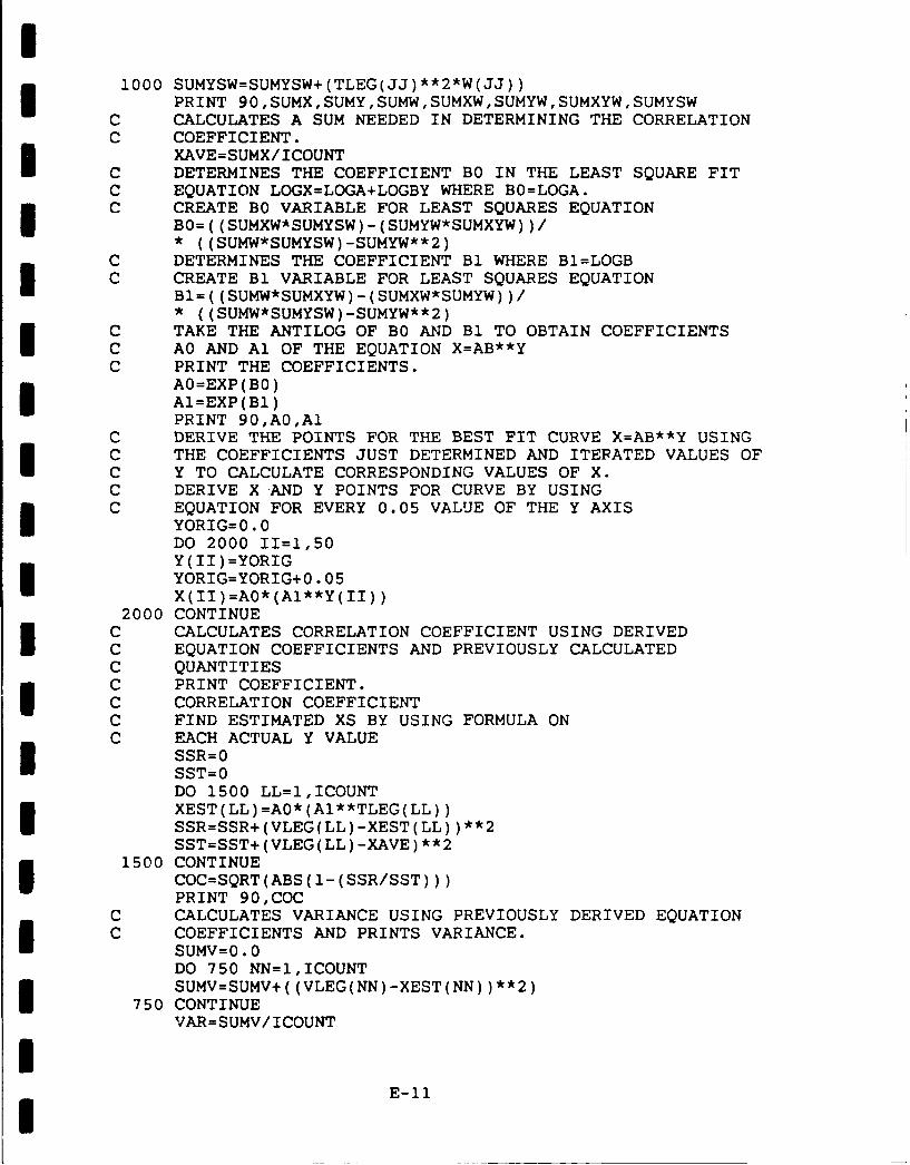
I1000 SUMYSW=SUMYSW+(TLEG(JJ)**2*W(JJ))
PRINT 90,SUMX,SUMY,SUMW,SUMXW,SUMYW,SUMXYW,SUMYSWC CALCULATES A SUM NEEDED IN DETERMINING THE CORRELATIONC COEFFICIENT.
XAVE=SUMX/ICOUNTC DETERMINES THE COEFFICIENT BO IN THE LEAST SQUARE FITC EQUATION LOGX=LOGA+LOGBY WHERE BO=LOGA.C CREATE BO VARIABLE FOR LEAST SQUARES EQUATION
BO=((SUMXW*SUMYSW)-(SUMYW*SUMXYW))/* ((SUMW*SUMYSW)-SUMYW**2)
C DETERMINES THE COEFFICIENT B1 WHERE B1=LOGBC CREATE B1 VARIABLE FOR LEAST SQUARES EQUATION
BI=((SUMW*SUMXYW)-(SUMXW*SUMYW))/* ((SUMW*SUMYSW)-SUMYW**2)
C TAKE THE ANTILOG OF BO AND B1 TO OBTAIN COEFFICIENTSC AO AND Al OF THE EQUATION X=AB**YC PRINT THE COEFFICIENTS.
AO=EXP(BO)AI=EXP(B1)PRINT 90,AO,AI
C DERIVE THE POINTS FOR THE BEST FIT CURVE X=AB**Y USINGC THE COEFFICIENTS JUST DETERMINED AND ITERATED VALUES OFC Y TO CALCULATE CORRESPONDING VALUES OF X.C DERIVE X AND Y POINTS FOR CURVE BY USINGC EQUATION FOR EVERY 0.05 VALUE OF THE Y AXIS
YORIG=0.0DO 2000 II=1,50Y(II)=YORIGYORIG=YORIG+0.05X(II)=AO*(AI**Y(II))
2000 CONTINUEC CALCULATES CORRELATION COEFFICIENT USING DERIVEDC EQUATION COEFFICIENTS AND PREVIOUSLY CALCULATEDC QUANTITIESC PRINT COEFFICIENT.C CORRELATION COEFFICIENTC FIND ESTIMATED XS BY USING FORMULA ONC EACH ACTUAL Y VALUE
SSR=0SST=0DO 1500 LL=1,ICOUNTXEST(LL)=AO*(AI**TLEG(LL))SSR=SSR+(VLEG(LL)-XEST(LL))**2SST=SST+(VLEG(LL)-XAVE)**2
1500 CONTINUECOC=SQRT(ABS(1-(SSR/SST)))PRINT 90,COC
C CALCULATES VARIANCE USING PREVIOUSLY DERIVED EQUATIONC COEFFICIENTS AND PRINTS VARIANCE.
SUMV=0.0DO 750 NN=1,ICOUNTSUMV=SUMV+((VLEG(NN)-XEST(NN))**2)
750 CONTINUEVAR=SUMV/ICOUNT
I ! E-ll
I
PRINT 90,VARC CALL VARIOUS CURVE PLOTTING AND TITLE PLOTTINGC RJUTINES, PLOT GRAPH AND BEST FIT CURVE WITH AXESC TITLES AND GRAPH TITLES.
ENCODE(70,ZTITLE) COC70 FORMAT(' CORRELATION COEFFICIENT EXPO= ',F5.3,'$')
ENCODE(80,YTITLE) AI,AO80 FORMAT(' A1=',F5.3,2X,'AO=',F5.3,5X,'X=AO*A1**Y$')
CALL CURVE(X,Y,50,0)CALL MESSAG(YTITLE,100,0.5,2.0)CALL MESSAG(ZTITLE,100,0.5,2.5)
90 FORMAT( )CALL ENDPL(1)RETURNEND
IIIIIIIIIIII
E-12I
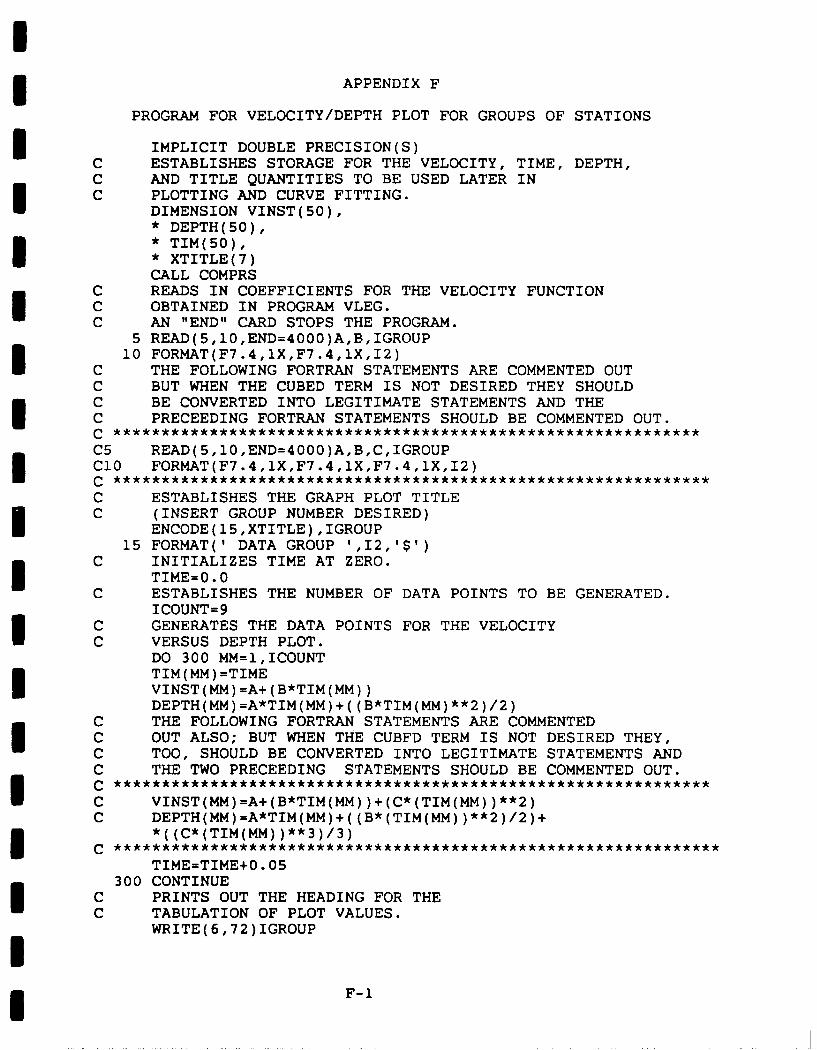
I
* APPENDIX F
PROGRAM FOR VELOCITY/DEPTH PLOT FOR GROUPS OF STATIONS
IMPLICIT DOUBLE PRECISION(S)C ESTABLISHES STORAGE FOR THE VELOCITY, TIME, DEPTH,C AND TITLE QUANTITIES TO BE USED LATER INC PLOTTING AND CURVE FITTING.
DIMENSION VINST(50),* DEPTH(50),* TIM(50),
* XTITLE(7)CALL COMPRS
C READS IN COEFFICIENTS FOR THE VELOCITY FUNCTIONC OBTAINED IN PROGRAM VLEG.C AN "END" CARD STOPS THE PROGRAM.
5 READ(5,10,END=4000)A,B,IGROUP10 FORMAT(F7.4,1X,F7.4,1X,I2)
C THE FOLLOWING FORTRAN STATEMENTS ARE COMMENTED OUTC BUT WHEN THE CUBED TERM IS NOT DESIRED THEY SHOULDC BE CONVERTED INTO LEGITIMATE STATEMENTS AND THEC PRECEEDING FORTRAN STATEMENTS SHOULD BE COMMENTED OUT.C *C5 READ(5,10,END=4000)A,B,C,IGROUPClo FORMAT(F7.4,1X,F7.4,1X,F7.4,1X,I2)CC ESTABLISHES THE GRAPH PLOT TITLEC (INSERT GROUP NUMBER DESIRED)
ENCODE(15,XTITLE),IGROUP15 FORMAT(' DATA GROUP ',12,'$')
C INITIALIZES TIME AT ZERO.TIME=0.0
C ESTABLISHES THE NUMBER OF DATA POINTS TO BE GENERATED.ICOUNT=9
C GENERATES THE DATA POINTS FOR THE VELOCITYC VERSUS DEPTH PLOT.
DO 300 MM=1,ICOUNTTIM(MM)=TIMEVINST(MM)=A+(B*TIM(MM))DEPTH(MM)=A*TIM(MM)+((B*TIM(MM)**2)/2)
C THE FOLLOWING FORTRAN STATEMENTS ARE COMMENTEDC OUT ALSO; BUT WHEN THE CUBFD TERM IS NOT DESIRED THEY,C TOO, SHOULD BE CONVERTED INTO LEGITIMATE STATEMENTS ANDC THE TWO PRECEEDING STATEMENTS SHOULD BE COMMENTED OUT.CC VINST(MM)=A+(B*TIM(MM))+(C*(TIM(MM))**2)C DEPTH(MM)=A*TIM(MM)+((B*(TIM(MM))**2)/2)+
*((C*(TIM(MM))**3)/3)C *
TIME=TIME+0.05300 CONTINUE
C PRINTS OUT THE HEADING FOR THEC TABULATION OF PLOT VALUES.
WRITE(6,72)IGROUP
F-i

I72 FORMAT(' DATA FOR GROUP ',12) I
C PRINTS OUT THE PLOT VALUES.DO 350 LL=1,ICOUNTWRITE(6,75)LL,DEPTH(LL),VINST(LL),TIM(LL)
75 FORMAT(' POINT NUMBER ',13,3X,' DEPTH 1,* F6.4,3X,' VELOCITY= ',F5.3,3X,' TIME= ',F4.2)
350 CONTINUEC CALLS THE PARABOLIC LEAST SQUARES CURVEC FITTING SUB PROGRAM.
CALL LEGPAX(VINST,DEPTH,ICOUNT,XTITLE)C CALL LSTPAX(VINST,DEPTH,ICOUNT,XTITLE)C CALLS THE PLOTTING ROUTINE.
CALL ENDPL(1)C RETURNS TO THE START OF THE PROGRAM TO PROCESSC ANOTHER SET OF DATA.I
GO TO 54000 CONTINUE
C ENDS THE PROGRAM.CALL DONEPLSTOPEND
IIIIIIIIII
F-2I
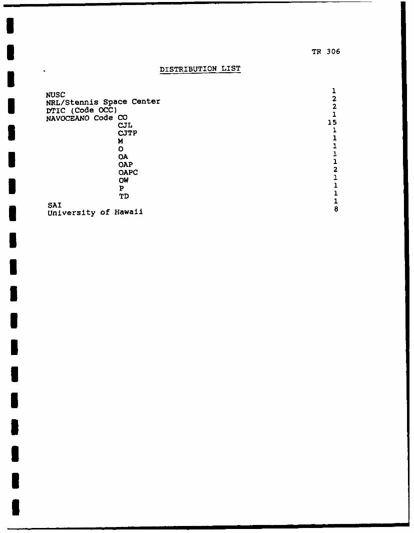
i TR 306
DISTRIBUTION LIST
NUSC 1
NRL/Stennis Space Center 2
I DTIC (Code OCC) 2
NAVOCEANO Code CO 1CJL 15CJTP 1M 10 1I OA 1
OAP 1OAPC 2
IOW 1
p 1TD 1
SAI 1
university of Hawaii 8
IiIIIIIIiII