Embed Size (px)
Citation preview
HAL Id: inria-00182005https://hal.inria.fr/inria-00182005
Submitted on 24 Oct 2007
HAL is a multi-disciplinary open accessarchive for the deposit and dissemination of sci-entific research documents, whether they are pub-lished or not. The documents may come fromteaching and research institutions in France orabroad, or from public or private research centers.
L’archive ouverte pluridisciplinaire HAL, estdestinée au dépôt et à la diffusion de documentsscientifiques de niveau recherche, publiés ou non,émanant des établissements d’enseignement et derecherche français ou étrangers, des laboratoirespublics ou privés.
Characterization of the Inevitable Collision States for aCar-Like vehicle
Rishikesh Parthasarathi
To cite this version:Rishikesh Parthasarathi. Characterization of the Inevitable Collision States for a Car-Like vehicle.[University works] 2006. �inria-00182005�

Master 2 Recherche
Imagerie, Vision et Robotique
Characterization of the Inevitable Collision
States for a Car-Like vehicle
Submitted By : Parthasarathi Rishikesh
Supervisor : Thierry Fraichard
Team: E-Motion
GRAVIR Laboratory
l’INRIA Rhône-Alpes


Abstract
Navigation is an important aspect of mobile robotics. Recently, we see a trend in roboticsystems leaving laboratories and clean rooms and moving to real world environments. Atthis point, it is critical to ensure the safety of the robotic system and the environment inwhich it moves.
In this work, the topic of “safe navigation” of a robotic system in a highly dynamicenvironment is considered. It is suggested that the dynamics of the robotic system andof the moving obstacles must be taken into account while performing navigation. It isillustrated that the idea of using a time-horizon for calculating a navigation plan doesnot guarantee safety. Developing on these points as the motivation, the novel concept ofInevitable Collision States (ICS) is introduced. An inevitable collision state is a statefrom which any action taken by the robotic system will lead to a collision. A theoreticalextension, the notion of imitating manoeuvres is proposed and proved to be efficient incalculating the ICS for a robotic system.
A case study involving the characterization of the ICS for a car-like vehicle is per-formed. A polynomial complexity algorithm complexity is proposed for an efficient com-putation of the ICS . The algorithm is implemented in C++. Experimental resultsobtained in various environments are presented.

Contents
Acknowledgements 1
1 Introduction and Overview 21.1 Motivations . . . . . . . . . . . . . . . . . . . . . . . . . . . . . . . . . . 2
1.1.1 Motivation 1: Considering Dynamics . . . . . . . . . . . . . . . . 41.1.2 Motivation 2: Avoiding Time-Horizons . . . . . . . . . . . . . . . 5
1.2 Objectives . . . . . . . . . . . . . . . . . . . . . . . . . . . . . . . . . . . 51.3 Contributions of the report . . . . . . . . . . . . . . . . . . . . . . . . . . 61.4 Report Outline . . . . . . . . . . . . . . . . . . . . . . . . . . . . . . . . 6
2 Literature Review 82.1 Basic Concepts . . . . . . . . . . . . . . . . . . . . . . . . . . . . . . . . 8
2.1.1 Configuration Space Formulation . . . . . . . . . . . . . . . . . . 82.1.2 State Space Formulation . . . . . . . . . . . . . . . . . . . . . . . 92.1.3 Configuration-Time Space Formulation . . . . . . . . . . . . . . . 102.1.4 State-Time Space Formulation . . . . . . . . . . . . . . . . . . . . 11
2.2 Deliberative Aprroaches . . . . . . . . . . . . . . . . . . . . . . . . . . . 122.3 Reactive Approaches . . . . . . . . . . . . . . . . . . . . . . . . . . . . . 12
2.3.1 Potential Field Approaches . . . . . . . . . . . . . . . . . . . . . . 132.3.2 Vector Field Histograms . . . . . . . . . . . . . . . . . . . . . . . 142.3.3 Dynamic Window Approach . . . . . . . . . . . . . . . . . . . . . 142.3.4 Linear Velocity Obstacles . . . . . . . . . . . . . . . . . . . . . . 15
2.4 k-step Approaches . . . . . . . . . . . . . . . . . . . . . . . . . . . . . . . 162.5 Conclusion . . . . . . . . . . . . . . . . . . . . . . . . . . . . . . . . . . . 17
3 Inevitable Collision States and Obstacles 193.1 Notations and Preliminary Definitions . . . . . . . . . . . . . . . . . . . 203.2 Inevitable Collision States and Obstacles . . . . . . . . . . . . . . . . . . 213.3 Calculating ICO(B) . . . . . . . . . . . . . . . . . . . . . . . . . . . . . 23
4 Case Study: Car-Like Vehicle 244.1 Characterization of the ICS . . . . . . . . . . . . . . . . . . . . . . . . . 24
4.1.1 Statement of the Problem . . . . . . . . . . . . . . . . . . . . . . 244.1.2 Trajectory Parameterization . . . . . . . . . . . . . . . . . . . . . 254.1.3 ICO calculation for a point obstacle moving in a straight line . . 264.1.4 ICO calculation for a solid obstacle moving in a straight line . . . 284.1.5 ICO calculation, for a stationary point and solid obstacle . . . . 28
1

4.2 On the Conservative Approximation . . . . . . . . . . . . . . . . . . . . . 294.3 Imitating Manoeuvres . . . . . . . . . . . . . . . . . . . . . . . . . . . . 30
4.3.1 Catching-up manoeuvre . . . . . . . . . . . . . . . . . . . . . . . 324.4 Catching-up manoeuvres for the car-like vehicle . . . . . . . . . . . . . . 32
4.4.1 ICO calculation for an obstacle moving in a straight line . . . . . 324.4.2 Optimal Control . . . . . . . . . . . . . . . . . . . . . . . . . . . 324.4.3 Optimal Catching-up Manoeuvre . . . . . . . . . . . . . . . . . . 33
5 Algorithm and Software Implementation 365.1 Algorithm for ICS-Checker . . . . . . . . . . . . . . . . . . . . . . . . . 36
5.1.1 Input . . . . . . . . . . . . . . . . . . . . . . . . . . . . . . . . . . 365.1.2 Output . . . . . . . . . . . . . . . . . . . . . . . . . . . . . . . . . 365.1.3 Algorithm . . . . . . . . . . . . . . . . . . . . . . . . . . . . . . . 365.1.4 Complexity of the Algorithm . . . . . . . . . . . . . . . . . . . . . 37
5.2 Software . . . . . . . . . . . . . . . . . . . . . . . . . . . . . . . . . . . . 385.2.1 Programming . . . . . . . . . . . . . . . . . . . . . . . . . . . . . 385.2.2 Experimental Results . . . . . . . . . . . . . . . . . . . . . . . . . 39
6 Conclusion and Future work 41
References 43
2

Acknowledgements
I would like to take this opportunity to thank a number of people who have played animportant role during the past one year. Firstly, I would like to thank the French Embassyof Singapore for granting me a scholarship to pursue my Masters degree in France andDr. Christian Laugier for giving me an opportunity to work in the E-Motion team.
I would like to thank my supervisor Dr. Thierry Fraichard for all the discussions,suggestions and guidance that he has provided me during this internship. I am sure thatI have learnt a lot about research from him. I would like to thank my colleague Ronanwhose every suggestion in programming improved my software. I also extend my thanksto Christopher and Pierre for discussions concerning various topics, including work.
Finally, I would like to thank Chen Cheng and Ronan for helping me proof-read thereport.
1

Chapter 1
Introduction and Overview
1.1 Motivations
Autonomous robotic systems are a major undertaking in robotics. In the recent years,robotic systems have started leaving laboratories, clean rooms, restricted environmentsand have started moving towards real world environments. Examples include indoor andoutdoor robots performing various tasks from sweeping floors (Probotics Cye-R, GeckoCarebot, iRobot Roomba, etc.), tour-guiding people in museums (Rhino, Minerva, Robox,etc.), helping people with disabilities, transporting humans in the form of intelligentvehicles in urban areas (Cycab, Parkshuttle), and traversing unstructured terrains (TheGrand DARPA Challenge) etc.
Autonomous system designing requires tackling a number of challenging problemsin perception, localization, modeling, reasoning under uncertainty, decision making, etc.Whatever the problem considered, the final decision is made on choosing a control actionto produce motion. Hence, motion is of prime importance in autonomous sytems. Themore sophisticated the applications become, the more concerned we ought to be aboutthe safety of these robotic systems and the environment in which these interact, be itwith people, vehicles or other autonomous systems. The characteristic of a real worldenvironment, irrespective of whether it is structured or unstructured, hostile or friendly, isthat it is dynamic. That is to say that it contains objects that move. The desired roboticsystem is expected to move in an environment that may contain moving obstacles, staticobstacles in the from of buildings etc.
If we would like to create robotic systems that can reach a destination with no or leasthuman intervention (by least human intervention we mean that the input descriptionswill only be what we want the vehicle to do rather than how to do it), we must be ableto achieve navigation (by navigation, we basically mean the problem of determining theelementary motion that the robotic system should perform during the next time-step) ina dynamic environment. As soon as the size and dynamics of the robotic system makeit potentially harmful to itself or it’s environment, the system should strive to avoidcollision. Now, as advancement in tourist guide vehicles and intelligent transportationvehicles continues, we must ask ourselves one important question. “How safe are thesevehicles in a dynamic environment with people, other moving obstacles ?” It is importantto understand this operational safety issue.
This is the focus of collision avoidance in motion planning and navigation. In fact
2
navigation approaches for mobile robotic systems can be broadly classified into threecategories, reactive, k-step and deliberative approaches. The deliberative approaches cal-culate a complete trajectory from the initial point to goal point. These can be computedoffline and there is no need to perform any additional obstacle avoidance at executiontime. A major disadvantage of these approaches is that they are too slow because of thecalculations involved in determining the obstacle-free space. Examples of deliberativeapproached include road-map approaches, cell decomposition, approximate cell decom-position [1], potential field approaches [2]etc.
A robotic system in a dynamic environment faces a hard real-time constraint and isobliged to make a decision within a bounded time. This constraint rules out the usage ofdeliberative approaches in navigation. Thus our study of real-time navigation in dynamicenvironments will mostly focus on the other two categories.
Reactive approaches, in contrast with deliberative approaches, generate only controlactions that are to be performed at the next time instant. The key advantage of thereactive methods is their low computational load which is particularly more importantin a dynamically changing environment. Reactive approaches perform the calculationsat execution time unlike the deliberative approach where obstacle avoidance is done off-line. This comes at an obvious disadvantage that they cannot yield optimal solutions.Another not so obvious disadvantage is the tendency to be stuck at local minima like inthe cases of Vector Field Histograms (VFH) [3] and its derivative VFH+ [4], potentialfield methods, Dynamic Window Approach [5] etc.
The primary concern of navigation is to ensure safety of the robotic system. Inan environment with moving obstacles this concern is critical as there is a necessity totake into concern the dynamics and the future behavior of the obstacles and the roboticsystem. A number of research papers [6], [7], [8] have addressed this issue. Another topicof interest under the framework of navigation is to incorporate the idea of a time horizonas in [7]. Before discussing the problems of incorporating a time-horizon, it is necessaryto explain how it is implemented or rather what characterizes a time-horizon. Let ussay we a model of the environment from the current time instant (t = 0) till t = ∞.If we use a time-horizon of say, t = 100, the model of the environment at t = 101 andthen on is just truncated. It is assumed that the model is not available. The reason forincorporating a time-horizon normally is mainly to reduce computational load. While[7], uses a time-horizon, [8] and [6] assume that a complete trajectory to the goal can becomputed when considering the dynamics of the robotic system and the moving obstacles.
The k-step approach is in between the deliberative and reactive approaches. Theseapproaches cater to the hard real time constraint and calculate a partial plan of k -steps.They also take into consideration the environment changes into their planning. Examplesinclude the Partial Motion Planning (PMP) scheme [9] and the VFH* [10] variation ofthe VFH method. PMP has an any-time flavor i.e., it returns the best trajectory whenrequested. In general, the look-ahead of k-step methods is shorter than deliberativeapproaches but better than reactive approaches and hence the chance of getting trappedin a local mininma is lower. They also claim that a complete trajectory to the goalcannot be calculated under hard real-time constraints. One important issue concerningthe k-step methods is that it is necessary to guarantee the safety of the system at theend of the k steps. By safety we mean that the system should not end in a state whereit cannot avoid a collision.
3

Before going into the safety issue in k -step methods, let us show that there is in facta need to consider the dynamics of the system and of the moving obstacles. We will alsodiscuss why it is correct to avoid using time-horizons in order to ensure safety of therobotic system. It takes a couple of simple examples such as the ones depicted in Fig. 1.1and Fig. 1.2 to illustrate this.
1.1.1 Motivation 1: Considering Dynamics
To explain the necessity of considering the dynamics of the system and of the movingobstacles, let us asumme the following case. A is considered to be a point mass capable oftranslating only to its right and is also capable of accelerating and decelerating. A is alsoassumed to be forward-moving only, as opposed to being able to reverse the direction ofmotion. The obstacle B is moving with a constant velocity vB in the opposite direction.
���������������������������������������������������������������
���������������������������������������������������������������
By
x
A
���������������������������������������������������������������
���������������������������������������������������������������
By
x
A
d(v)
����������
� � � � � � � � � � � � � � � � � � � � � � � � � � �
���������������������������������������������������������������
By
x
d(v)
A
d(B) d(B)
Figure 1.1: A translates along x without any rotation. The obstacle B (striped re-gion)translates with constant velocity -vB along the x axis. The plane (x,y) denotes Wwhere the objects move. a) The case where both A’s dynamics and B’s dynamics arenot considered. b) A’s dynamics is alone considered. c) The case where the dynamics ofboth A and B are considered.
Let us now discuss the different cases where dynamics of the objects in the workspaceare either considered or neglected.
Not considering any system dynamics:
If the system dynamics of A and B are not considered, then the region occupied by theobstacle is the only forbidden area. In Fig.1.1a, this is represented by the striped area.In this case, the precaution is to not be inside this striped area.
Considering only the dynamics of A
If the dynamics of A alone is considered, we will take into account the distance d(v) inFig, 1.1b,that it takes A to break according to the current velocity. This produces theextended region of B along the direction of A’s velocity. It is obvious that the dynamicsor the future motion of the obstacle are not taken into consideration and the precautionis not to be inside this new area from where A cannot stop before hitting B.
Considering the dynamics of both A and B
In this case, both A’s and B’s dynamics are taken into consideration. We will havethe distance d(v) that it takes A to break according to the current velocity and alsothe distance B will travel d(B). Hence the collision region is a distance d(v) + d(B)
4

(Fig, 1.1c,)from the current position of B. This is bad news since A is already in thisregion. Hence a collision with B is inevitable.
Hence, if a naive collision avoidance system that doesn’t take into consideration boththe dynamics of A and of B is used, it would assume that the current state is safe andwould eventually lead to a collision. This simple but neat example emphazises the lackof safety in most of the current algorithms in literature like [5],[10],[2],[3] etc.
1.1.2 Motivation 2: Avoiding Time-Horizons
When it comes to the issue of time-horizon, it is argued that whenever a robotic systemdecides it future motion by restricting the reasoning to a finite time-horizon, collisions maypotentially happen beyond this time-horizon and safety is not guaranteed. This argumentis supported with the following example. Let us consider the example in Fig.1.2
Figure 1.2: A is in a situation to choose one among the four trajectories. In reality,trajectory A is the only safe trajectory, but incorporation of a time-horizon at h2 makesB a safe trajectory and at h1 makes C a safe trajectory, which are obviously fatal.Example taken from [11].
Now in our example, it is assumed that A can choose between four trajectories onlyto reach it’s goal, A,B,C or D. Evaluating each of these trajectories with a time-horizonat h1, leads A to eliminate trajectory D and choose between A,B and C. If B or C isunfortunately chosen, A is definitely in trouble. It should be noted that increase of thetime-horizon will not solve the problem. Only a time-horizon infinite or at least greaterthan the time to reach the goal state guarantees A’s safety (assuming that A can restsafely at the goal).
1.2 Objectives
The main objective of this project is to consider the dynamics of the robotic system,the dynamics of the moving objects and to avoid the incorporation of a time-horizon innavigation. The navigation method that will be used is the k-step navigation. Althoughtechnically sound and computationally fast, the key question that arises whenever we usek-step methods is How sure can we be that the system will never end up in a state (at theend of k-steps) from where a collision is inevitable?.
5

The solution proposed in this document is the concept of Inevitable Collision States(ICS) introduced in [12]. An ICS for a robotic system is a state for which, no matterwhat the future trajectory is, a collision eventually occurs. So the safety of the system isguaranteed by never being in an ICS . A theoretical solution for the safety of a roboticsystem is offered in Chapter 3.
1.3 Contributions of the report
The basic study of this concept was done in [13]. Formal definitions of the inevitablecollision states and obstacles, properties fundamental for their characterisation and casestudy with simple static objects, etc were introduced in [12]. This report extends thisconcept to moving objects.
On the theoretical side, the concept of imitating manoeuvres that produce a compactapproximation of the ICS is proposed. These manoeuvres are suitable for systems thatare capable of reproducing the trajectory of the obstacles. They are comprised of acatching-up part, in which the system orients itself along the direction of the obstacle,and an imitating part, in which the system follows the control inputs of the obstacle. Itis proved that the ICS region depends on the time taken for the catching-up part. Anoptimization procedure that uses bang-controls is performed to take the robotic systemthrough the catching-up part as fast as possible, thus reducing the ICS region as muchas possible. This concept is further explored to encompass braking trajectories, a popularconcept in collision avoidance literature, as a special case of imitating manoeuvres.
On the practical side, the ICS concept is applied to a car-like vehicle case study. Analgorithm for an ICS-Checker is proposed. In short, the algorithm is a predicate ICS(s)that returns true if and only if the state s is an ICS . The algorithm has a polynomialcomplexity. The algorithm is implemented in software with the braking trajectories andimitating manoeuvres. Typical environments, both cluttered and highly dynamic, aredefined. Examples include a highway scenario and a city scenario with pedestrians andbuildings etc. A maze environment for a cycle, which could be considered as the piano-mover problem’s (in configuration space) equivalent in state space, is also presented. Theidea is to calculate if a given trajectory is collision free or whether there exists a safetrajectory.
1.4 Report Outline
This document is organized as follows.
• Chapter 2 introduces the basic concepts and formalization for solving navigationproblems. A literature review details the current state of the art. Although variousalgorithms exist, only algorithms that are relevant to the one proposed in thisdocument are reviewed. This chapter concludes with a statement of problem forwhich a solution is proposed in this document.
6

• Chapter 3 introduces the concept of Inevitable Collision States (ICS) and formaldefinitions of the inevitable collision states and obstacles are presented. Propertiesfundamental for their characterisation are established.
• Chapter 4 describes the characterization the ICS for a car-like vehicle. Extensionsto the concepts in Chapter 3 (concept of imitating manoeuvres) are proposed. Theproposed concept is extensively detailed and it’s capability to improve the qualityof conservativeness in approximating the ICS is theoretically proved.
• Chapter 5 discusses the overall algorithm for generating the ICS region and alsofor collision-checking in the form of predicate ICS(s). A software implementationof the proposed algorithm is then described. Typical environments and classicalproblems are introduced and implemented using the software. A laborious analysisof the complexity of the algorithm is performed.
• Chapter 6 concludes the document, and proposes ideas for further work that canbe performed.
7

Chapter 2
Literature Review
The robotics literature presents many approaches to collision-free motion for robots.They are generally categorized according to their underlying methodology. Historically,navigation was generally an off-line task, as only stationary environments were considered.Methods used were also purely geometry-based. The problem was formalized in highdimensional spaces rather than the workspace W. The advantage is that the roboticsystem can be replaced by a point in higher dimensions and hence navigation for thesystem is reduced to a problem involving a point object. An extensive review is providedin [1].
Research in this area is mature and the notion of configuration space (C) proposed in[14] has been the most successful way of solving these problems. Later extensions to thisformulation resulted in the notion of State space (S), Configuration-Time space (CT ),State-Time space (T S) etc, according to whether the dynamics of the robotic system andmoving obstacles are taken into consideration.
2.1 Basic Concepts
2.1.1 Configuration Space Formulation
The underlying idea of the C-space is to represent A as a point in an appropriate space-A’sC-space, and to map the obstacles in this space. This mapping transforms the problemfrom plannin a motion for a dimensioned object, in this case A, to planning a motion fora point object in the new space. In other words, it make the constraints on the motionsof A more explicit.
Notion of C-space
Let A be represented as a closed polygonal region, a subset of W , the workspace, whichin turn is the physical space on which A moves. W is either R2 or R3 as the case may be.The obstacles Bi’s are considered fixed closed polygonal regions of W.FA is the movingframe with A and FW is fixed. By definition, since A is rigid, every point a in A has afixed position in FA. But a’s position in W depends on the position of FA in FW . TheBi’s are fixed and hence every point on each Bi has a fixed position w.r.t FW .
8

A configuration q of A is a set of parameters that uniquely determine the positionof every point on A. In other words, q specifies the position and orientation of FA inFW . The set of all configurations q’s forms the configuration space C, and a configurationis represented as a point in C. A configuration q is collision-free if A placed at q doesnot collide with obstacles in the workspace or with itself. The free configurations form asubset F of C.
The configuration space of a robotic system is the appropriate framework to addresspath planning problems where the focus is on the geometric aspects of motion planning(no collision between the system and the fixed obstacles of the workspace).
Obstacles in C-space
The Bi’s in the previous section were the workspace image of the obstacles. To plan apath in the configuration space, the obstacles have to be mapped to the C-space. Everyobstacle Bi in W maps in C to a region:
CBi = {q ∈ C/A(q) ∩ Bi 6= ∅} (2.1)
This region CBi is called the C-obstacle of Bi. The union of all the C-obstacles:
q⋃
i=1
CBi (2.2)
is called the C-obstacle region and the set
Cfree = C/q⋃
i=1
CBi = {q ∈ C/A(q) ∩ (q⋃
i=1
Bi) = ∅} (2.3)
is called the free space. Any configuration q in Cfree is called a free configuration.
Figure 2.1: Obstacle representation in configuration space
2.1.2 State Space Formulation
Notion of S-Space
The C-space is apt for geometric path planning, i.e., it takes into consideration thekinematic constraints of A but as soon as we talk about real systems like vehicles, the
9

dynamic constraints like maximum velocity and acceleration. play a critical role. TheS-space takes into consideration these constraints. Or in other words the S-space hasboth the C-space parameters and their derivatives for parameters. In the most generalcase it could be s = (x, y, θ, v).
Obstacles in S-space
The obstacles whose image in W are Bi’s map to a region SBi in S.
SBi = {s ∈ S/A(s) ∩ Bi 6= ∅} (2.4)
This region is also called the S-obstacle of Bi. The union of all the S-obstacles:
N⋃
i=1
SBi (2.5)
is called the S-obstacle region and the set
Sfree = S/N⋃
i=1
SBi = {s ∈ S/A(s) ∩ (N⋃
i=1
Bi) = ∅} (2.6)
is called the free space. Any state s in Sfree is called a free state. Not surprisingly, theSBi is same as the CBi for all obstacles. This is due to the fact that irrespective of thevelocity or other derivative parameters of C that are incorporated in S, as long as theposition is the same there is a collision. For example, it does not matter if the collisionbetween A and Bi takes place when A has a velocity vA = 0 or 50 m/s.
2.1.3 Configuration-Time Space Formulation
Notion of CT -space
The C and S-space formulation of the motion planning does not extend to deal with timeconstraints, for example, if some of the Bi’s are moving, the CBi corresponding to theobstacle is time-dependant. Hence, there is a need to incorporate the time dimension.The easiest extension is the CT -space [1]. Here, Bi(t) represents the region of W occupiedby Bi at time t and we assume that the regions Bi(t) are known ∀ i. This assumptionrequires that the future behavior of the obstacles is not affected by the movement of A.
Obstacles in CT -space
Now, since the location of the C-obstacles may vary with t, it impossible to representthem in C, in such a way that we can still reduce the motion of A to the motion of apoint among fixed constraints. Hence we add the time dimension to C. This results in thenew space CT =C x [0,+∞). A maps in CT to a configuration-time (q,t) meaning thatA’s configuration at time t is q. Every obstacle Bi maps in CT to a stationary regionCT Bi called a CT -obstacle defined by:
CT Bi = {(q, t)/A(q) ∩ Bi(t) 6= ∅} (2.7)
10

Figure 2.2: A translates freely without any rotation in the plane. The obstacle B trans-lates at fixed orientation with constant velocity vB between the time instants t1 and t2.vB is parallel to the y-axis and points upwards. At any other time t /∈ [t1, t2], B is mo-tionless. The CT -obstacle is obtained by sweeping CB along a line that is perpendicularto the xy-plane when t /∈ [t1, t2] and oriented along the vector (0, vB, 1) when t ∈ [t1, t2].
Fig.2.2 shows an example of obstacle representation in the CT -space. We define freespace in CT as:
CT free = CT /N⋃
i=1
CT Bi (2.8)
2.1.4 State-Time Space Formulation
The T S-space is a tool to formulate problems of trajectory planning in dynamic workspaces.This concept was proposed in [15]. T S-space permits the study of the different aspects ofdynamic trajectory planning, i.e. moving obstacles and dynamic constraints in an unifiedway. It stems from two concepts we have already seen: the CT -space and the S-space,the space of the configuration parameters and their derivatives. In this framework, theconstraints imposed by both the moving obstacles and the dynamic constraints can berepresented by static forbidden regions.
A state-time of A is represented by adding the time dimension to a state, henceit is represented as A(s,t). As explained in the case of S, where the S-obstacles wassame as the C-obstacles, here again we have the T SB same as the CT -obstacle. On theother hand, a state-time (s,t) is admissible if and only if it does not violate the dynamicconstraints on the maximum velocities and acceleration.
In fact in order to perform navigation, we are not obliged to follow the above men-tioned formulations. For example, most of the recent algorithms in the literature do notalways use these formulations, but other notions of space, for example the velocity spaceetc (e.g., Velocity obstacles, [7], Dynamic Window Approach, [5], Global Dynamic Win-dow Approach, [16] etc,) but a knowledge of these formalizations is important to analyseand understand the different approaches.
11

2.2 Deliberative Aprroaches
C-space formulations were widely used during the 80’s. Navigation methods like theVisibility graph method, Retraction method, Freeway method, Silhouette method, [1]calculate the obstacle free area of C which is then used for motion planning. The interestedreader is referred to [1] for an extensive review of these algorithms.
Advantages
On the whole, these algorithms share an advantage in the sense that, the safety issue istaken care of during the free space calculating stage. Hence it is done only once and canbe performed off-line.
Disadvantages
• A major disadvantage is that the calculation of free space is computationally veryexpensive. In higher dimensions, it is almost impossible to capture the free spaceconnectivity.
• A second disadvantage is that, if the assumed model of the environment changes to asmall extent, the free space connectivity is altered. Hence it has to be re-calculated.This is a major issue especially in highly dynamic environments.
Hence, global methods are not of much practical use for a dynamic environment andfor the same reason we will not go into the details of these methods.
2.3 Reactive Approaches
These methods calculate only a local (small region around the robotic system) free spaceconnectivity rather than the entire free space connectivity.
Advantages
• The locality is a characterisitc feature of reactive methods that helps reduce thecomputational effort.
• Dynamic environments and static environments are given same treatment.
• It is easy to incorporate reactive methods with a motion planner such that we canrapidly verify if a state is a collision state, unlike the deliberative methods.
Disadvantages
• The reactive nature of the algorithms make them susceptible to local minima prob-lems and sometimes may not be able to reach the goal, if used with a motionplanner.
• The path calculated by a reactive motion planner is not an optimal solution. Hencethis is an issue if the problem requirement demands an optimal solution.
12

Despite these disadvantages, reactive methods are the only methods that can work indynamic environments and can be incorporated with motion planners. Few algorithmsthat perform reactive navigation are reviewed below.
2.3.1 Potential Field Approaches
Potential Field methods introduced in [2], can be classified under both the categoriesof deliberative and reactive methods depending on the potential function involved. Forexample, a simple distance from the goal potential would only result in a reactive methodetc. More complex potentials (with special attention to degenerate cases) can make ita global method. Using the notion of C-space, A is viewed as a point. A path in thisspace is constructed by exploring the C-space with heuristics. The heuristics used in thepotential field method is based on the physical potentials. Obstacles exert a repulsiveforce on A and the goal exerts an attractive force. All potentials at each point in C areadded vectorially to produce a resultant force acting on that point. This potential valueimplicitly defines a path by acting as a direction value. The path then forms a gradientdescent to the goal.
Figure 2.3: a)Workspace W, also the C-space in this case, containing two obstacles. b)After calculating the attractive and repulsive forces at each point of C.
Advantages
• The path is not calculated in advance; rather the path is implicitly represented bythe potential function. Hence, the computational complexity is low and motioncommands can be generated very easily.
Disadvantages
• In some cases, there is a possibility that the net force on the robot sums up to bezero at places other than the goal position. Although these cases can be dealt withseparately by providing a slight motion (considering it as a degenerate case of thealgorithm) in some direction, there are other possibilities of the robot being stuckin the local minima.
13

• No consideration is given to the dynamics of A and of the moving obstacles. Hencethe same reasoning in Section 1.1.1 is applicable here.
2.3.2 Vector Field Histograms
This methods compute a direction for A to head in (action to be performed at the nexttime step), in W or C. The inputs to the algorithm are the sensor values at time instant t.The controller builds a histogram (Vector Field Histogram (VFH) [3], VFH+ [4], VFH*[10] etc,) using the sensor values and looks for gaps in the histograms which could helpin identifying possible directions of motion. This method is very efficient for identifyinga directional command for collision-free movement in real-time.
Certain defects of the first proposed VFH method were identified and rectified in thefuture versions. For instance, VFH+ considers the size of the robot and expands theobstacles in the histogram (quite similar to idea of C-spaces, but does not explicitly buildthe configuration space), it also takes into account the robot trajectory using parameterslike the minimum steering radius etc. Finally, it uses a cost function to determine thebest action among the available (maximum of three) actions.
Disadvantages
• This method too does not take into account the dynamics of the robot, and theobstacles.
• Another problem with the VFH methods in general is that they build the histogramin the angle space. They also choose an action in the wide collision-free angle space.This could be a problem, for example, when the robot is near an obstacle even asmall collision-free distance will be seen as a large collision-free angle. On the otherhand, if the robot is far from the same opening, it will regard the same collision-freedistance as a small collision-free angle.
2.3.3 Dynamic Window Approach
This approach proposed by [5] works on the velocity space of the robotic system A. Theadvantage of working in the velocity space is that the kinematic and dynamic constraintscan easily be taken into consideration by restricting the search space only to the reachablevelocity space. The search space is the set of tuples (v, ω) the translational and rotationalvelocities that are achievable by A. Among all the tuples, those are selected that, ifselected and executed would allow A to come to a stop before hitting the obstacle. Thesevelocities are called admissible velocities.
The search is further restricted by a dynamic window giving this method the name.This reflects the dynamic limitations of A, i.e. given A’s current velocity and accelerationcapabilities, the dynamic window has those velocities that can be achieved within a giventime interval. Fig.2.4 illustrates the subdivision of the search space in the DWA.
Disadvantages
• The DWA does not take into consideration the dynamics of the obstacles although
14

Figure 2.4: Search space in the DWA. The space of all possible velocity commandsis divided into admissible and blocked regions. The small rectangle corresponds to thedynamic window consisting of velocities reachable by A within the specified time interval.
it takes into account the dynamics of the robotic system. The disadvatages of notconsidering the dynamics of the obstacles was already illustrated in Fig.1.1. Thesame problem exists here.
The reactive nature of this algorithm was overcome by the Global Dynamic WindowApproach in [16], but even this method does not take into consideration any dynamics.
2.3.4 Linear Velocity Obstacles
This interesting method proposed in [7], assumes that all obstacles in W move alongarbitrary trajectories and their instantaneous state (position or velocity) are known or atleast measurable (model assumption). Like the DWA, this method too operates in thevelocity space. A and all Bs are assumed to be circular, so that C is easy to calculate.A colliding relative velocity cone is defined with respect to every moving obstacle (as theCB s are always circular, it is definitely a cone). Velocities in this cone lead to a collisionwith the obstacle at arbitrary times. This is calculated for all Bs in W. This whole setof velocities forms the set of non-admissible velocities.
The dynamic constraints are used to reduce the search space to only the set of reach-able velocities depending on the acceleration limits and current velocity of A. The com-plement set of the non-admissible velocities in the set of reachable velocities is the set ofvelocities that avoid all obstacles.
Fig.2.5 shows geometrically how the non-admissible velocities region is calculated.
Advantages
• This is one of the few algorithms that takes into consideration the dynamics of bothA and Bs. Hence it does not suffer from the short comings discussed in Section1.1.1.
15

Figure 2.5: Velocity space in the VO. The space of all velocity commands is dividedinto admissible and non-admissible regions. Here RVC is the relative velocity cone thatwill lead to a collision between A and B constituing the non-admissible region. B has avelocity vB shown as vb. To calculate the absolute velocity of A that induces a collision,a Minkowski sum is performed between RVC and vb. Hence, here velocity va1 avoids acollision with B while velocity va2 causes a collision.
• The method is computationally very efficient as the search space is not high-dimensional (velocity space).
• It can take into account any number of obstacles, both dynamic and stationary.
• The motion command is generated as a velocity selected from the set of reachableadmissible velocities which in turn is generated using simple boolean operations onsets.
Disadvantages
Although this is one of the most popular and efficient methods, the following problem isidentified.
• For implementation issues, the VO method uses a time-horizon th calculated usingthe distance proximity between obstacles and A. The idea is based on clipping theset of non-admissible velocities, with th i.e.. all velcoties that lead to a collisionafter th are moved to set of admissible velocities. This is a typical situation asshown in Fig.1.2. Collision free trajectory is gauranteed until time th but we haveno idea if we can find another velocity after time th to gaurantee collision. Hencefor the reasons mentioned in Section 1.1.2, this method too does not ensure safety.
2.4 k-step Approaches
These approaches bridge the gap between the deliberative and reactive approaches. Theirlook ahead is more than the latter but less than the former. Instead of planning only the
16

next time instant, they plan a few steps (say k) ahead. Such an extension to the VFH+method discussed in Section 2.3.2 resulted in VFH*, which tries to address the issue ofthe susceptibility to local minima. VFH* takes into account the local nature of VFHi.e., the lack of a look ahead, and circumnavigates the problem by building a search treeat a given robot position. It takes into consideration the primary candidate directions(current action) and the projected candidate directions (future actions) by constructinga VFH+ histogram at each projected state to bring in a flavor of look-ahead.
Even though some of these work address real time motion planning a few only considerhighly changing environment, performing fast replanning using probabilistic techniques,though for simple systems e.g., [6] and [17]. It is argued in [9] that when complex roboticsystems and environments are considered, the real time constraints have to be explicitlyinto account in the form of a time-bound for making a decision, etc. In such a case acomplete trajectory to the goal cannot be computed in general and only partial plans canbe found. They have thus introduced the Partial Motion Planning (PMP) method withan any-time flavor that returns the best trajectory planned (till that instant) wheneverit is polled for a solution. This is the framework that this project assumes for navigation.
On the other hand, when dealing with partial plans, it becomes of the utmost im-portance to consider the behaviour of the system at the end of the trajectory. What ifa car ends its trajectory in front of a wall at high speed? It becomes clear that strongguarantees should be given to this trajectory in order to handle the safety issues raisedby such a partial planning.
Hence, there is a need for a collision-checker module that takes in a state si of therobotic system as input and produces a boolean output as to whether si is safe. Now,how do we define safe for a robotic system in a dynamic environment?
Def. 1 A state si is defined as safe iff it is not already in collision with an obstacle andthere is at least one control input φi ∈ Φ, such that, the terminal state sj, the result ofapplying φi at si is also safe.
This work proposes a collision-checker that takes into consideration the dynamics of thesystem and of the moving obstacles, does not incorporate a time-horizon and returns aboolean value for a state verifying if it is safe.
2.5 Conclusion
The methods we have reviewed in this chapter have their own merits and de-meritsaccording to their respective assumptions. In general, the earliest reactive methods didnot take into account the dynamics of the system, or the dynamics of the obstacles. Themethods using the velocity space take into account the dynamics and the kinematics,thanks to the simplicity of the velocity space. But these methods use a time horizonwhich leads to problems mentioned in Section 1.1.2. How can we be sure that afterchoosing a velocity and executing it, we can always find another velocity in the reachableadmissable region at the next time instant? What if we end the trajectory at an instantwhere the set of reachable admissible velocities is a null set? This ambiguity caused bythe time-horizon is one that this work aims to overcome.
17

Hence, in conclusion, there is a need to develop a navigation algorithm that takesinto consideration the dynamics of the robot and of the moving obstacles and does notincorporate a time horizon. The navigation approach taken in this project is the PMPframework, and the collision checker proposed is the Inevitable Collision State-checkeror, ICS-checker. The theoretical framework for calculating the ICS is presented in thenext Chapter.
18

Chapter 3
Inevitable Collision States andObstacles
An inevitable collision state, proposed in [12] for a robotic system can be defined as astate for which, no matter what the future trajectory followed by the system is, a collisionwith an obstacle eventually occurs. An inevitable collision state takes into account thedynamics of both the system and the obstacles, fixed or moving. This concept is verygeneral and can be useful both for navigation and motion planning purposes: for its ownsafety, a robotic system should never find itself in an inevitable collision state.
����������������������������������������
������������������������
PSfrag replacements
P
Wall
v
d(v)
Collision states
xW
yW
W Inevitable collision states
Figure 3.1: Collision states vs inevitable collision states.
Consider Fig.3.1, let P be a point mass that can only move to the right with a variablespeed. A state of P is characterised by its position (x, y) and its speed v. If the workspaceW features a wall, the states whose position corresponds to the wall are obviously collisionstates. On the other hand, assuming that it takes P a certain distance d(v) to slow downand stop, the states corresponding to the wall and the states located at a distance lessthan d(v) left of the wall are such that, when P is in such a state, no matter what itdoes in the future, a collision will occur. These states are inevitable collision states forP . Clearly, for P ’s own safety, when it is moving at speed v, it should never be in oneof these inevitable collision states. The size of the inevitable collision states region, i.e.the grey region located to the left of the wall, depends on the distance d(v) which inturns depends on the current speed of P . Assuming that d(v) varies linearly with v, thecomplete set of inevitable collision states is a prism embedded in the state space S of P(Fig.3.2).
In general, an inevitable collision state for a given robotic system can be defined as astate for which, no matter what the future trajectory followed by the system is, a collision
19

�������������������������������������������������������
�������������������������������������������������������
PSfrag replacements
xS
yS
vS
S
d(v)v
Collision states
Inevitable collision states
Figure 3.2: Full representation in the xyv state space S of P of the inevitable collisionstates corresponding to the situation depicted in Fig.3.1.
eventually occurs with an obstacle of the environment. Similarly, it is possible to definean inevitable collision obstacle as the set of inevitable collision states yielding a collisionwith a particular obstacle.
3.1 Notations and Preliminary Definitions
Before defining the inevitable collision states and obstacles, useful definitions and nota-tions are introduced. Let A denote a robotic system. It is assumed that its dynamicscan be described by a differential equation such as: s = f(s, u) where s ∈ S is the stateof A, s its time derivative and u ∈ U a control. S and U respectively denote the statespace and the control space of A. Let φ ∈ Φ denote a control input, i.e. a time-sequenceof controls. φ represents a trajectory for A. Starting from an initial state s0 (at time 0)and under the action of a control input φ, the state of A at time t is denoted by φ(s0, t)
Given a control input φ and a state s0 (at time 0), a state s is reachable from s0 by φiff ∃t, φ(s0, t) = s. Let R(s0, φ) denote the set of states reachable from s0 by φ. Likewise,R(s0) denotes the set of states s reachable from s0, i.e. such that ∃φ, s ∈ R(s0, φ):
R(s0, φ) = {s ∈ S|∃t, φ(s0, t) = s}
R(s0) = {s ∈ S|∃φ, s ∈ R(s0, φ)}
Introducing φ−1(s0, t) to denote the state s such that φ(s, t) = s0, it is possible todefine R−1(s0) (resp. R−1(s0, φ)), as the set of states from which it is possible to reachs0 (resp. to reach s0 by φ):
R−1(s0, φ) = {s ∈ S|∃t, φ(s, t) = s0 ⇔ φ−1(s0, t) = s}
20

R−1(s0) = {s ∈ S|∃φ, s ∈ R−1(s0, φ)}
Let WB denote an obstacle. When WB is moving, WB(t) represents the subset of Woccupied by WB at time t. When WB is fixed, the time index is omitted: ∀t,WB(t) =WB(0) = WB . Every obstacle has an image in the state space: the set of states yielding acollision between the robotic system and an obstacle WB(t) determines the state obstacleof WB(t) which is denoted B(t). B(t) = {s ∈ S|A(s)∩WB(t) 6= ∅}, where A(s) denotesthe closed subset of W occupied by A in state s. Once again, when WB is fixed, thetime index is omitted. A state s is a collision state at time t iff ∃B, s ∈ B(t). In this case,s is a collision state at time t with B.
The document places itself in the state space framework unless otherwise mentioned.For the sake of simplicity, state obstacles are called obstacles only and the time index isindicated only when necessary.
3.2 Inevitable Collision States and Obstacles
Based on the definitions and notations introduced in the previous section, the inevitablecollision states and the inevitable collision obstacles are formally defined.
Def. 2 (Inevitable Collision State) Given a control input φ, a state s is an in-
evitable collision state for φ iff ∃t such that φ(s, t) is a collision state at time t.Now, a state s is an inevitable collision state iff ∀φ, ∃t such that φ(s, t) is a collisionstate at time t. Likewise, s is an inevitable collision state with B for φ iff ∃t suchthat φ(s, t) is a collision state at time t with B. Finally, s is an inevitable collision
state with B iff ∀φ, ∃t such that φ(s, t) is a collision state at time t with B.
Def. 3 (Inevitable Collision Obstacle) Given an obstacle B and a control input φ,ICO(B, φ), the inevitable collision obstacle of B for φ is defined as:
ICO(B, φ) = {s ∈ S|s is an inevitable collision state with B for φ}
= {s ∈ S|∃t, φ(s, t) is a collision state at time t with B}
= {s ∈ S|∃t, φ(s, t) ∈ B(t)}
Now, ICO(B), the inevitable collision obstacle of B, is defined as:
ICO(B) = {s ∈ S|s is an inevitable collision state with B}
= {s ∈ S|∀φ, ∃t, φ(s, t) is a collision state at time t with B}
= {s ∈ S|∀φ, ∃t, φ(s, t) ∈ B(t)}
Based upon the two definitions above, the following property can be established. Itshows that ICO(B) can be derived from the ICO(B, φ) for every possible control inputφ.
21

Property 1 (Control Inputs Intersection)
ICO(B) =⋂
ΦICO(B, φ)
Proof:
s ∈ ICO(B) ⇔ ∀φ, ∃t, φ(s, t) is a collision state at time t with B
⇔ ∀φ, s ∈ ICO(B, φ)
⇔ s ∈⋂
ΦICO(B, φ)
Assuming now that B is the union of a set of obstacles, B =⋃
i Bi, the followingproperty can be established. It shows that ICO(B, φ) can be derived from ICO(Bi, φ)for every subset Bi.
Property 2 (Obstacles Union)
ICO(⋃
i
Bi, φ) =⋃
i
ICO(Bi, φ)
Proof:
s ∈ ICO(⋃
i Bi, φ) ⇔ ∃t, φ(s, t) is a collision state at time t with⋃
i Bi
⇔ ∃Bi, ∃t, φ(s, t) is a collision state at time t with Bi
⇔ ∃Bi, s ∈ ICO(Bi, φ)
⇔ s ∈⋃
i ICO(Bi, φ)
Combining the two properties above, the following property is derived. It is theproperty that permits the formal characterisation of the inevitable collision obstacles fora given robotic system.
Property 3 (ICO Characterisation) Let B =⋃
i Bi,
ICO(B) =⋂
Φ
⋃
i
ICO(Bi, φ)
Proof:
ICO(B)1=
⋂
ΦICO(B, φ)
2=
⋂
Φ
⋃
i
ICO(Bi, φ)
22

Consider property 1 (and property 3), it establishes that ICO(B) can be derived fromthe ICO(B, φ) for every possible control input φ. In general, there is an infinite numberof control inputs which leaves little hope of being actually able to compute ICO(B).Fortunately, it is possible to establish a property which is of a vital practical value sinceit shows how to compute a conservative approximation of ICO(B) by using a subset onlyof the whole set of possible control inputs.
Property 4 (ICO Approximation) Let I denote a subset of the set of possible controlinputs Φ,
ICO(B) ⊂⋂
I
ICO(B, φ)
Proof:
ICO(B)1=
⋂
I∪I
ICO(B, φ)
=⋂
I
ICO(B, φ) ∩⋂
I
ICO(B, φ)
⊆⋂
I
ICO(B, φ)
3.3 Calculating ICO(B)
Given A’s state space equation, in order to calculate the ICO for the obstacles in W ,we move on to the S-space of A. Initially we decide on the control inputs that willbe considered to approximate the ICO. These can be (but are not limited to) brakingtrajectories, where A starts at the current state si and breaks until the velocity is zero.The braking trajectories also depend on A’s dynamic and kinematic constraints.
Next we calculate the ICO(Bi, φj) for each obstacle in W and take the union of thesesets for each φj in Φ. Then we calculate the intersection of all these sets to identify theICO for each obstacle.
The interest of these properties to characterise inevitable collision obstacles for ob-stacles in W appears in the next chapter which discusses a car-like vehicle case study.
23

Chapter 4
Case Study: Car-Like Vehicle
A car-like vehicle is a typical example of system subject to kinematic constraints sinceit cannot translate and rotate freely in the workspace W. The constraints affecting themotion of a car-like robotic system translate into an equation and an inequation involvingthe velocity parameters of the robot. They are said to be non-holonomic. They do notrestrict the set of configurations reachable from a given configuration, but they do restrictthe space of velocities achievable at any configuration of the robotic system which followsthe constraint below,
y cos θ = x sin θ (4.1)
where x and y are the coordinates of the midpoint R between the two rear wheels andθ ∈ [0, 2π) is the angle between the x-axis of FW attached to the workspace and mainaxis of the car. This is shown in the bicycle model in Fig.4.1.
PSfrag replacements
x
y
θ
ξ
v
b
Figure 4.1: The car-like vehicle A (bicycle model).
4.1 Characterization of the ICS
4.1.1 Statement of the Problem
Let us consider a robotic system A that moves like a car-like vehicle and whose dynamicsfollow a bicycle model. A state of A is defined by the 4-tuple s = (x, y, θ, v) where (x, y)
24

are the coordinates of the rear wheel, θ is the main orientation of A, and v is the linearvelocity of the front wheel (Fig. 4.1). A control of A is defined by the couple (uξ, uv)where uξ is the steering angle and uv the linear acceleration. The motion of A is governedby the following differential equations:
x = v cos θ cos uξ
y = v sin θ cos uξ
θ = v sin uξ/bv = uv
with |uξ| ≤ ξmax and |uv| ≤ uvmax. b is the wheelbase of A. A moves on a planarworkspace W cluttered up with a set of polygonal obstacles WB i. Although the statespace S of A is four-dimensional, it is not attempted to compute the inevitable collisionobstacles in the full four dimensional state space. Instead, the structure of S is exploitedand the inevitable collision obstacles are computed in two-dimensional slices of S only.The slices considered are slices with constant θ and v. Such slices are interesting becauseit is straightforward to compute, for such a slice, the state obstacles Bi.
4.1.2 Trajectory Parameterization
The trajectory of a car-like robot with non-zero steering angle and constant velocity canbe parameterized in terms of its (v0,θ0) slice, where v0 and θ0 are the initial values ofvelocity and orientation. Considering this slice we can integrate the above differentialequations to get,
θ(t) = θ0 +v0
bsin uξt (4.2)
x(t) = x(0) +b
tanuξ(sin(θ0 +
v0
bsin uξt) − sin θ0) (4.3)
y(t) = y(0) −b
tanuξ(cos(θ0 +
v0
bsin uξt) − cos θ0) (4.4)
Detecting collision states
Thanks to these equations, it is easy to find the position of A at time t = 0 for collisionwith the obstacle at any arbitrary time t. We just need to backpropagate in time from thevalues of Bx(t) and By(t) for (x(t),y(t)) and solve for (x(0),y(0)). Thus, s0=(x(0),y(0))is an ICS for B for this control input.
Now, let ICOI(B) denote⋂
I ICO(B, φ). ICOI(B) is the conservative approximationof ICO(B). In order to calculate the ICS , only a finite subset I of the whole set ofpossible control inputs Φ is considered (Property 4). The subset I selected contains thecontrol inputs φ of arbitrary duration with constant steering angle uξ and constant linearacceleration uv. First, I is split into two subsets IS and IT corresponding respectively tocontrol inputs for which A is moving straight, i.e. uξ = 0, and control inputs for whichA is turning, i.e. uξ 6= 0. Then, the set of control inputs IξT is introduced. It is the setof control inputs for which A is turning with the steering angle uξ.
25

4.1.3 ICO calculation for a point obstacle moving in a straightline
Let B be a moving point obstacle. Recall that B(t) gives the position of B at time t.In order to characterize ICO(B), we consider B as the union ∪tB(t). We proceed tocalculate ICO(B, φ) = ∪tICO(B(t), φ). Now, according to Definition 2 in Section 2,ICO(B(t), φ) is the set of states s such that if A starts from s (at time 0) and is subjectto the control input φ it reaches B(t) (at time t). Such a state s belongs to R−1(B(t), φ)and is actually the unique solution of the equation φ(s, t) = B(t) ⇔ s = φ−1(B(T ), t).Hence, in conclusion ICO(B, φ) = ∪tφ
−1(B(t), t)
Computing ICOI
ξ
T
(B) (A is turning)
Now, to calculate the ICS for a uξ analytically, we need to find all states in the (θ, v)slice from where ∃tA(t) ∩ B(t) 6= ∅. This is nothing other than solving the equations 4.3and 4.4 for various values of t. Solving for x(0) and y(0) we obtain the result illustratedin Fig.4.2.
0 5 10 15 20 25 30 35 40 45 50−8
−6
−4
−2
0
2
4
6
8
0 5 10 15 20 25 30 35 40 45 50−8
−6
−4
−2
0
2
4
6
8
Figure 4.2: Left: ICOIξ
T
(B) when A is turning with constant uξ and zero uv. The line
across the curve is the trajectory of the obstacle. A’s velocity vA is assumed to be twotimes that of the obstacle’s velocity vB . Right: The same situation except, here A is
turning with constant uξ and decelerating with a braking distance d(v)
The curve on the left is a cycloid. On the right is ICOIξ
T
(B). When A is turning
and decelerating it collides with B iff it is on a collision course and its distance to Bi isless than the braking distance d(v). The straight line part is due to the fact that, whenvA is zero, it stops on the path of the obstacle. This control input is also known as thebraking trajectory.
Generalizing for all steering commands
We repeat the same process for the extreme steering angles (maximum positive andmaximum negative angles). Now, the analysis is complete except that it lacks the ICO(B)characterization for straight motion of A (uξ = 0), which is the topic of the next section.
26

Computing ICOIs(B) (A is moving straight)
Again, we have to parameterize the trajectory of A by time t. Generalization to otherslices is direct. The main issues we have to take into consideration are cases in whichvA(t) ≤ 0, 0 < vA(t) < vAMax
,vA(t) ≥ vAMaxaccording to whether A is decelerating
or accelerating. vAMaxhere is A’s maximum velocity and vA(t) = vi + uvmaxt, gives the
velocity at time t. Like in the case of steering angles, here too, we consider trajectorieswith maximum acceleration and deceleration only.In the decelerating case, as we consider forward moving car-like robot, we don’t allowvA(t) < 0. Hence, as long as vA(t) > 0,
y(t) = y(0) − v0t+1
2uvmaxt
2 (4.5)
where, v0 is the (v,θ) slice we are considering and uvmax is absolute value of the maximumdeceleration. But if vA(t) = 0
y(t) = y(0) +v0
2
2uvmax(4.6)
In the accelerating case, we shouldn’t allow vA(t) > vAMax. Hence, as long as vA(t) <
vAMax
y(t) = y(0) − vt−1
2uvmaxt
2 (4.7)
But if vA(t) = vAMax, then
y(t) = y(0) − vAMaxt (4.8)
Using these equations, we get an ICO(B) characterization as shown in Fig.4.3 for thestraightline motion of A.
0 1 2 3 4 5 6 7 8 9 10−60
−50
−40
−30
−20
−10
0
10
maximum deceleration
constant velocity
maximum acceleration
obstacle trajectory
Figure 4.3: ICOIS(B) when A is moving straight (uξ=0) with maximum acceleration,
uvmax, constant speed, uv=0, and maximum deceleration, -uvmax. The straight line y=0, isthe obstacle’s trajectory.
27
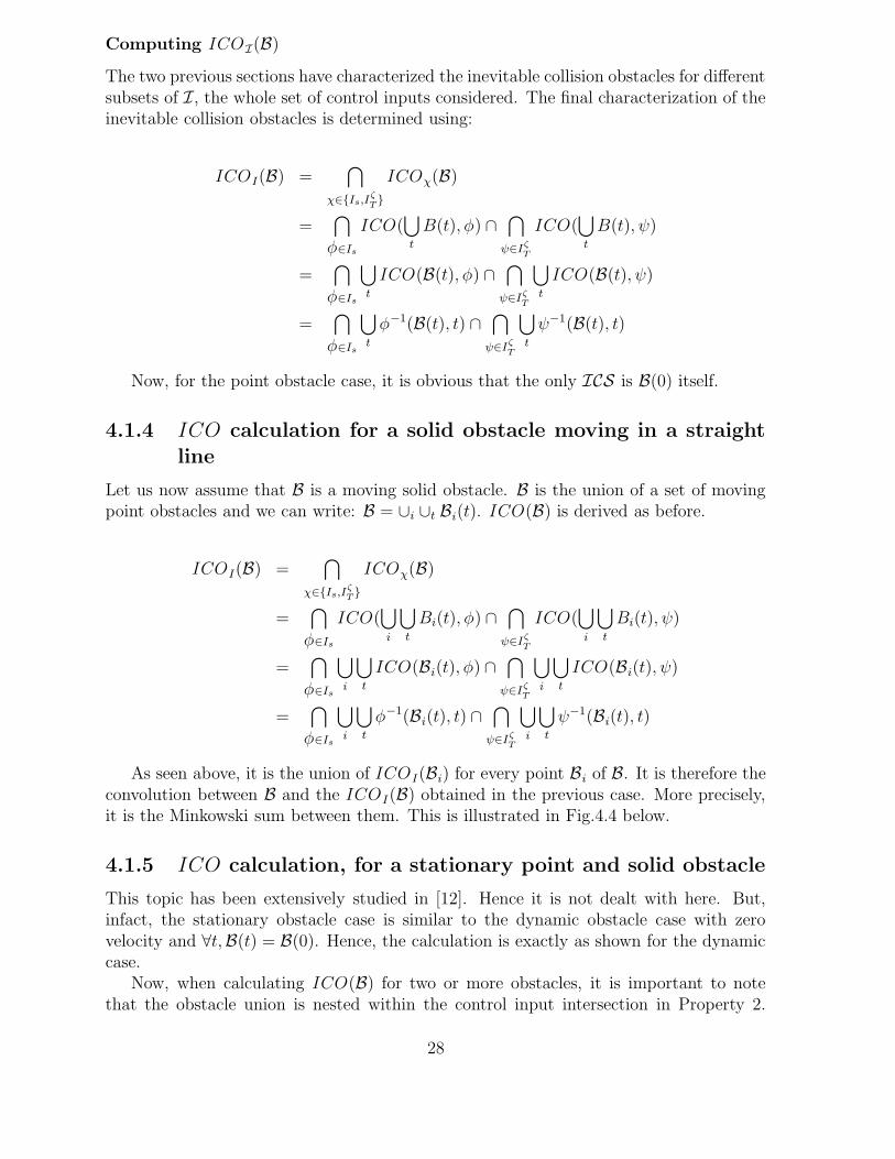
Computing ICOI(B)
The two previous sections have characterized the inevitable collision obstacles for differentsubsets of I, the whole set of control inputs considered. The final characterization of theinevitable collision obstacles is determined using:
ICOI(B) =⋂
χ∈{Is,Iζ
T}
ICOχ(B)
=⋂
φ∈Is
ICO(⋃
t
B(t), φ) ∩⋂
ψ∈Iζ
T
ICO(⋃
t
B(t), ψ)
=⋂
φ∈Is
⋃
t
ICO(B(t), φ) ∩⋂
ψ∈Iζ
T
⋃
t
ICO(B(t), ψ)
=⋂
φ∈Is
⋃
t
φ−1(B(t), t) ∩⋂
ψ∈Iζ
T
⋃
t
ψ−1(B(t), t)
Now, for the point obstacle case, it is obvious that the only ICS is B(0) itself.
4.1.4 ICO calculation for a solid obstacle moving in a straightline
Let us now assume that B is a moving solid obstacle. B is the union of a set of movingpoint obstacles and we can write: B = ∪i ∪t Bi(t). ICO(B) is derived as before.
ICOI(B) =⋂
χ∈{Is,Iζ
T}
ICOχ(B)
=⋂
φ∈Is
ICO(⋃
i
⋃
t
Bi(t), φ) ∩⋂
ψ∈Iζ
T
ICO(⋃
i
⋃
t
Bi(t), ψ)
=⋂
φ∈Is
⋃
i
⋃
t
ICO(Bi(t), φ) ∩⋂
ψ∈Iζ
T
⋃
i
⋃
t
ICO(Bi(t), ψ)
=⋂
φ∈Is
⋃
i
⋃
t
φ−1(Bi(t), t) ∩⋂
ψ∈Iζ
T
⋃
i
⋃
t
ψ−1(Bi(t), t)
As seen above, it is the union of ICOI(Bi) for every point Bi of B. It is therefore theconvolution between B and the ICOI(B) obtained in the previous case. More precisely,it is the Minkowski sum between them. This is illustrated in Fig.4.4 below.
4.1.5 ICO calculation, for a stationary point and solid obstacle
This topic has been extensively studied in [12]. Hence it is not dealt with here. But,infact, the stationary obstacle case is similar to the dynamic obstacle case with zerovelocity and ∀t,B(t) = B(0). Hence, the calculation is exactly as shown for the dynamiccase.
Now, when calculating ICO(B) for two or more obstacles, it is important to notethat the obstacle union is nested within the control input intersection in Property 2.
28

Figure 4.4: Left: ICOI(B) for A, taking into account both IS and IT . So, whenever Afinds itself in the highlighted region at t = 0, it will eventually collide with B. Right:ICOI(B) for A in the case of two obstacles. Notice regions r1, r2 and r3. From r1,all control inputs lead to collision with B1, similarly from r2 with B2 but from r3, somecontrol inputs lead to a collision with B1 and others with B2.
Theoretically, this property is complete for computing the ICO(B), but in some cases, asthe one shown in Fig.4.4b, we find regions of ICS , (for example r1 r2 and r3 in this case).Among these regions, r3 is created due to the intersection of infinite strips of ICO(B) fordifferent control inputs leading to collision with different obstacles.
4.2 On the Conservative Approximation
In fact, every point in the set of ICS has it’s own time-to-collision and most often, ICSthat lie far away from the obstacles are mainly due to collision after a long time. Statesin these regions (e.g. r3), although correctly characterized as ICS for the considered setof control inputs, I, can be made to vanish by considering a larger set I
′
, (shown later).On the other hand, regions r1 and r2 can only be reduced (by considering many controlinputs) but not made to vanish unless we assume trajectories uncharacteristic to A.
This issue could be easily fixed by incorporating a time-horizon, but the objective ofthis project is precisely to avoid the notion of time-horizon as it renders the system unsafe.How else could we get rid of these regions which are too conservative an approximation?First, we begin by defining conservativeness which will help us formalize this issue.
Def. 4 A set of control inputs I is considered to be more conservative than a set I ′
iff VOI > VOI′, where VO is the volume of the ICS region calculated using these controlinputs.
It is to be noted that the VO not only depends on the cardinality of set I but also thequality of the control input in evading the obstacles. The fact that VO is minimum(VOmin) in the case where we consider the set of all possible control inputs, (practicallyinfinite) is evident. We call this volume to be conservative of order zero, or exact ICS .Hence the lower the order, the smaller the volume (closer to the exact ICS). In the samelines, we also define the quality of the approximation.
29

Def. 5 The quality of the approximation of a set of control inputs I is given as the ratioVOmin/VOI . A quality value of 0 means the approximation is too conservative, while aquality of 1 is the best one can achieve.
Now, getting back to the question, is it possible to completely get rid of ICS that arefar away from the obstacles, only by considering a fixed number of control inputs?. Theanswer is no, as will be seen below.
Property 5 If the number of control inputs considered for the robotic system is fixed,the quality reduces with increase in the number of obstacles.
Proof: Assume I = {I1,I2} be the set of all control inputs available to the roboticsystem and ∀φ ∈ I1, ∃t, φ(s0, t) ∈ B1(t) and ∀ψ ∈ I2, ∃t, ψ(s0, t) ∈ B2(t), or in otherwords, state s0 is an ICS .
Now, let G =⋂
I1 ICO(B1(t), φ) ∩⋂
I2 ICO(B2(t), ψ). G defines the set of states fromwhere one set of control inputs lead to a collision with one obstacle and another setof control inputs lead to a collision with another obstacle. Now, to avoid this region,we can add another trajectory φnew to I in such a way that G ∩ ICO(B1(t), φnew) andG ∩ ICO(B2(t), φnew) = ∅.In other words, this seems to provide a solution that theaddition of the new trajectory avoids the region G. But, now let us fix the number ofcontrol inputs, and start adding obstacles to W . Theoretically it is easy to carefully placean obstacle, to make G ∩ ICO(B3(t), φnew) 6= ∅
Thus as we keep on adding obstacles to W , the order of conservativeness increases i.e.the ICS volume increases. The main reason for this behavior is the presence of infinitestrips of ICO’s. Hence, there is a need to have a control input that produces only a finiteICO(B) region. To this we introduce the idea of imitating manoeuvres.
4.3 Imitating Manoeuvres
Imitating manoeuvres are control inputs in which the robot tries to imitate the obstacle’strajectory. They consist of two parts:
• The “catching-up” part, during which the robot from an arbitrary state tries toachieve a zero relative velocity with the obstacle.
• The “following” part, during which the robot duplicates the obstacle’s control in-puts.
The interest in these imitating manoeuvres is that, the ICO(B) for these control inputstend to cloud around a fixed radius of the obstacle (under the condition that the roboticsystem is physically capable of duplicating the obstacle’s trajectory).
The Fig.4.5 illustrates this idea. A is the robotic system and B is the obstacle. Theyhave the same velocity and orientation (zero relative velocity). Hence in this case, thereis no need for a catching-up manoeuvre. If from this time instant, A applies the samecontrol inputs as B (the following manoeuvre), they will have a collision iff A(0) andB(0) intersect. In other words, ICO(B) region is finite and limited only to B(0). On theother hand, A’ and B have a non-zero relative velocity. To have a finite ICO(B) region,
30

W
B
Acatching−up
A’
Figure 4.5: A and B have the same velocity and heading angle. Heading angle of A’is different. The catching-up manoeuvre consists of orienting A’ with B in the shortestpossible time. W denotes the workspace.
a catching-up manoeuvre is necessary (shown as the dotted line). Once the catching-upmanoeuvre is successfully accomplished, the following manoeuvre is executed.
This is analytically proved below.
Property 6 A catching-up manoeuvre that results in a zero relative velocity between therobotic system A and the obstacle B gives rise to a finite ICO(B) region.
Let tc denote the catching-up time, φc denote the control input corresponding to thecatching-up manoeuvre and φf denote the control input corresponding to the followingmanoeuvre (φf is same as the obstacle’s control inputs).
Proof:
ICO(B) =⋃
t
ICO(B(t))
=⋃
0≤t≤tc
ICO(B(t), φc) ∪⋃
t≥tc
ICO(B(t), φf)
=⋃
0≤t≤tc
φc−1(B(t), t) ∪ φc
−1(⋃
t≥tc
φf−1(B(t), t))
=⋃
0≤t≤tc
φc−1(B(t), t) (4.9)
It is clear that the ICO(B) is the union of the ICO(B) due to the catching-up and thefollowing manoeuvre. When the robotic system has the same control inputs as that of theobstacle, the following manoeuvre’s ICO(B) reduces to φc
−1(B(tc), tc) (because for twoobjects having a zero relative velocity a collision can take place only if they start at thesame point on the workspace. Thus the ICO(B) is reduced to a finite region representedby the first term based on the catching-up manoeuvre alone.
31

4.3.1 Catching-up manoeuvre
The key to have a good quality ICS region is to avoid infinite strips of ICO(B). This isaccomplished by the imitating manoeuvre. In fact, the following inferences can be madefrom Property 6:
• If the robot is capable of reproducing the obstacles behavior, a combination of acatching-up and following manoeuvres can improve the quality of ICS approxima-tion.
• The catching-up part is different for different slices of the (v,θ) plane and hence itis of prime importance to characterize it in terms of v and θ values.
• And, the shorter the time taken by the catching-up manoeuvre is, the smaller theICO region.
With these points, we can go ahead to define the best possible manoeuvre for therobot to execute the catching-up manoeuvre in the shortest possible time.
4.4 Catching-up manoeuvres for the car-like vehicle
4.4.1 ICO calculation for an obstacle moving in a straight line
Consider a (v0,θ0) slice in the (v,θ) space. The equation that relates the change in θ valuew.r.t time is given as,
θ(t) = θ0 +v0t sin(uξ)
b(4.10)
Consider an obstacle B moving in a straightline with an orientation θobs and velocity vobs.The distance to be travelled by A to reach the orientation is fixed at r(θobs-θ0), the lengthof the arc Larc, where r = b
tan(uξ). According to the previous section, the idea of the
catching-up manoeuvre is to make the relative velocity between A and B zero as soon aspossible. This makes it neccessary to accelerate or decelerate according to whether v0 islesser or greater than vobs respectively. But what exactly is the optimal way to cover thedistance and satisfy the velocity constraint at the same time ?
4.4.2 Optimal Control
According to the Pontryagin Maximum Principle [18], optimal controls are typically hardlimited and piecewise continuous. That is to say that, they are hard against the constraintboundaries and switch abruptly between limits at certain critical points in the time axis.These optimal controls are also called Bang-Bang controls for the same reason.
A simple example of bang-bang control is to cover a fixed distance starting fromrest state and stopping at the final state in the shortest possible time. The solution forthis problem is to accelerate as hard as possible to reach maximum speed (MaximumAcceleration Phase), travel as fast as possible for as long as we can (Maximum VelocityPhase) just in time to brake as hard as possible to stop at the destination (MaximumDeceleration Phase), all assuming that the distance is large enough to allow all three
32

phases to be executed. The bangs divide the problem into sub-tasks and the optimalsolution is locally optimal in the sense that at each instant we should do as well as wecan for the current subtask to achieve a globally optimal solution.
4.4.3 Optimal Catching-up Manoeuvre
In our case, the catching-up manoeuvre can hence be characterized in three phases, phaseI to reach vAMax
from vA (not from 0 like in the example), phase II at the maximumvelocity and phase III to reach vobs (not 0 again).
1. Phase I: Time needed to accelerate to vAMax
t1 =vAMax
− v0
uvMax
(4.11)
2. Phase III: Time needed to decelerate to vB
t3 =vB − vAMax
−uvMax
(4.12)
3. Distance traveled in Phase I
d1 = v0t1 +1
2uvMaxt
21 (4.13)
4. Distance traveled in Phase III
d3 = vAMaxt3 −
1
2uvMaxt
23 (4.14)
5. Time needed to reach the vB from v0
tAB =|v0 − vB|
uvMax
(4.15)
6. Distance traveled in time t0B
d0B = v0t0B ±
1
2uvMaxt
20B (4.16)
± according to whether v0 is greater or lesser than vB
Now, with these constraint equations, we have the following equations to verify thefeasibility of executing the three phases.
1. d1 + d3 < LarcIn this case, A should execute Phase II for t2 = Larc−(d1+d3)
vAMax
seconds. This is
illustrated in Fig.4.6
2. d1 + d3 = LarcIn this case, A cannot execute Phase II, and hence t2 = 0, but A will reach therequired velocity and orientation.
33

Ac
Velocity
VB
VA
Vs
As
Vmax
T1+T2+T3T1 T1+T2 Ts time
Af
Figure 4.6: Velocity-Time graph of A. (vB is the velocity of the obstacle (to be achieved
at the end of the catching up manoeuvre),v0 is the current velocity of the A, (vs, Ts) thevelocity of A and the best time to cover the distance (maximum acceleration all the way).The time taken by the catching up manoeuvre is Tf = t1 + t2 + t3, where t1 is the timetaken to reach maximum velocity, t2 is the time traveled at maximum velocity and t3 isthe time taken to decelerate to vB from the maximum velocity. Although the best time
Ts is shorter than Tf , it is to be noted that the speed Vs (> vAMax) is not attainable by
A. To travel an equivalent distance of Larc, the area Af should be equal to As. Area Ac
denotes the common area. Obviously, As + Ac = Larc
3. d1 + d3 > LarcIn this case, A will actually travel a distance of d1 +d3−Larc in the direction of themotion of the obstacle if we want to execute both phases I and III to completion.But the optimal solution is to accelerate for a time t′1 (< t1) and then decelerate tovB in time to exactly cover the distance. This is a special case and we will need towork out the following possibilities.
• For the sub-case where d0B < Larc, the optimal solution is as explained above.
Two cases exist, one when v0 < vB and the other when v0 > vB . It isnecessary to find ti that gives an area equal to the distacne to be traveled.Fig.4.7a. illustrates this case
• On the other hand, the case where d0B > Larc occurs when the distance
traveled on applying the control action (maximum acceleration or deceleration)to reach the vB is already greater than the length of the arc. In this case it is
best (the only option) to provide control action to reach vB and a distance ofd
0B − Larc is traveled along the trajectory of the obstacle. This is explainedin Fig.4.7b.
34

ToTi Ts Tf
Af
VB
VA
Vi
Vs
Ac
D2O
As
time
Velocity
To
Af
VB
VA
D2O
time
Velocity
Vs
As
Ts =Tf
Figure 4.7: Velocity-Time graph of A. a) (vB , To) are the velocity of the obstacle (to be
achieved at the end of the catching up part) and the time taken to attain this velocity(directly) resp. (vs, Ts) are the velocity of A and the best time to cover the distance(maximum acceleration all the way) resp. and (vi, Ti) the maximum velocity which alsosatisfies property 1, and time to reach this velocity. The time taken by this catchingup manoeuvre is Tf . To travel an equivalent distance of Larc, the area Af should beequal to As. Area Ac denotes the common area. Obviously, As + Ac = Larc. b) Hered
0B > As+ Ac = Larc, hence Tf = To
Finally, we have to calculate the ICO for the imitating manoeuvre for every obstacleBi in the scene. An example of the imitating manoeuvre for an obstacle moving in astraight line is shown below in Fig.4.8. Notice the finite ICO(B) region.
ICO(B)
Y
X
A
B
Figure 4.8: Obstacle B is moving in a straight line towards the right. A has an headingangle of θ=90. The catching-up manoeuvre consists of reaching a state where θ is 0and v is vB in the shortest time possible. The following manoeuvre consists of applying
zero linear acceleration. The finite region of ICO(B) is the set of states from where thecatching-up trajectory would lead to a collision.
In conclusion, this Chapter has studied the characterization of ICS for a car-likevehicle and proposed the concept of imitating manoeuvres that are critical for the qualityof the approximation of the ICS set. The next Chapter describes an algorithm for thesoftware implementation of this case-study.
35

Chapter 5
Algorithm and SoftwareImplementation
This Chapter presents an algorithm to realize the ICS characterization for a car-likevehicle discussed in Chapter 4. The proposed algorithm is then implemented in software.A complexity analysis shows that collision checking can be performed in polynomial time.
5.1 Algorithm for ICS-Checker
The algorithm takes the form of a predicate ICS(si) that is true iff si is an ICS .
5.1.1 Input
• si, the state that is to be checked for collision. The values passed are xi,yi,θi andvi. Here (xi,yi) is the workspace position of A and (θi,vi) are the heading angleand velocity of A respectively. (They also correspond to an unique slice in the4-dimensional state space).
• A set B of Ns static obstacles and Nd dynamic obstacles, the positions in the caseof static obstacles and the predicted future behavior (velocity and heading angle)in the case of dynamic obstacles.
5.1.2 Output
A boolean value saying whether si is an ICS .
5.1.3 Algorithm
By definition, whenever A is inside the region ICO(B) at time 0, no matter what actionit takes, it eventually collides with B. Hence, when the ICS checker (collision checker) isprovided with a state si (which will be reached by A at time t′), the time axis is translatedto commence from t′ as 0 and the obstacle’s positions at t = t′ are assumed to be theirpositions at 0 and the ICO(B) is calculated. And, if si is inside this calculated regionICO(B) at time 0 (t′), we return a boolean value true to signify that si is infact an ICS .
36

After adding imitating manoeuvres, the ICO characterization in Section 4.1.4 is al-tered as,
ICOI(B) =⋂
χ∈{I∫ ,ITζ ,IE}
ICOχ(B) (5.1)
=⋂
φ∈I∫
ICO(⋃
i
⋃
t
Bi(t), φ) ∩⋂
ψ∈ITζ
ICO(⋃
i
⋃
t
Bi(t), ψ) ∩⋂
µ∈IE
ICO(⋃
i
⋃
t
Bi(t), µ)
=⋂
φ∈I∫
⋃
i
⋃
t
ICO(Bi(t), φ) ∩⋂
ψ∈ITζ
⋃
i
⋃
t
ICO(Bi(t), ψ) ∩⋂
µ∈IE
⋃
i
⋃
t
ICO(Bi(t), µ)
=⋂
φ∈I∫
⋃
i
⋃
t
φ−1(Bi(t), t) ∩⋂
ψ∈ITζ
⋃
i
⋃
t
ψ−1(Bi(t), t) ∩⋂
µ∈IE
⋃
i
⋃
t
µ−1(Bi(t), t)
where, I is the complete set of control inputs considered, Is is the sub-set of controlinputs where A moves in a straight line, IζT is the sub-set of control inputs where Amoves in with a non-zero steering angle, and IE is the sub-set of imitating manoeuvres.The cardinality of each sub-set is explained in the next section.
Steps involved in calculating the ICS for a given (θ, v) slice
1. Minkowski Sum calculation: The obstacles are grown w.r.t the θ slice of the vehicle.
2. ICO calculation for each obstacle: Calculate ICO(B,φ) for any one point on eachobstacle. The control inputs considered for each obstacle are,
• Braking trajectories with steering angles {−uξmax, 0, uξmax}. (3 control inputs)
• Trajectory with maximum acceleration uvmax.(this considerably reduces theICO for a dynamic obstacle).
• Imitating manoeuvre of each dynamic obstacle. (Nd control inputs)
3. Minkowski Sum calculation: The obstacles are further grown by calculating theminkowski sum between the ICO generated by the control inputs for the pointconsidered and the grown obstacle in step 1.
4. In case of more than one obstacle, calculate ICO(B, φj) =⋃Ni=1
⋃
t ICO(Bi(t), φj),where N = Nd + Ns is the number of obstacles, for ∀j = 1 . . .M control inputswhere M = Nd + 4, the total number of control inputs.
5. Calculate⋂M
φj=1ICO(B, φj) to find the ICO(B) or the ICS for the slice
6. Point Location: Check if the workspace position (x, y) is inside the ICS region
5.1.4 Complexity of the Algorithm
1. Step 1 of the algorithm: Let nB and nA be the number of vertices of the obstacles(all obstacles together) and the vehicle respectively, the minkowski sum then has acomplexity of O(nB + nA) if both polygons are convex, O(nBnA) if one of them is
37

convex and the other non-convex and O(n2BN
2A), if both of them are non-convex. In
our implementation, although we have a choice of considering vehicles of any type,in the general case a rectangle representation of the vehicle is chosen. Hence thecomplexity is O(4nB) or O(nB).
2. Step 2 of the algorithm: While calculating the ICO for any point, we use arcs (withknown radius and arc length) and straight lines as a part of the trajectory. Hence,we add 1 vertex to denote the end of the arc (the arc begins at the point on theobstacle) and another to denote the end of the straight line (the line begins at theend of the arc). Hence for each point on the obstacle, we add a maximum of O(M)points for M control inputs.
3. Step 3 of the algorithm: In this step, the minkowski sum between the grown ob-stacles in step 1 and the trajectories in step 2 is performed. The result of step 1is generally not convex, neither is the result of step 2. Hence the complexity isO(M2n2
B)
4. Step 4 of the algorithm: Union and intersection operations can be computed inO(nlogn + klogn), where n is total number vertices of the two polygons and k isthe complexity of the output. In our case, M(N − 1) union operations will haveto be performed. In the worst case, there are nB vertices for each union operation.Hence the complexity is O(nBlognB + klognB) for each union operation and step 4has a complexity of O(MN(nBlognB + klognB)). A constraint on N , the numberof obstacles is that, N ≤ nB/3 as all polygonal obstacles have atleast 3 vertices.Hence the complexity of calculating the union is O(MnB(nBlognB + klognB))
5. Step 5 has the same complexity as step 4.
6. Step 6, the point location query has a complexity O(logn), where n is the numberof vertices. In our case the maximum number of vertices is O(M 2n2
B)
5.2 Software
The above mentioned algorithm has been implemented in software, typical environmentshave been defined, for example, highway environment with lanes, and a maze environmentfor a cycle, that could be considered as the piano-mover problem’s equivalent in statespace, are proposed.
5.2.1 Programming
The programming is done using C++ and the graphics interface was designed usingFLTK [19]. Commercially available software like LEDA [20] etc, have built-in functionsto perform the steps highlighted in the algorithm. In this project no commercial softwarewas used. The source codes for the Minkowski sum, Planar point localization etc, wereadapted from [21] and changed to suit the application.
38

Environment Number of Number of Total number ExecutionStatic obstacles Dynamic obstacles of vertices time (in ms)
Highway 8 4 48 ≈ 98 8 64 ≈ 17.58 16 96 ≈25
Maze 2 0 8 ≈ 14 0 16 ≈ 1.58 0 32 ≈2
Table 5.1: Execution time
5.2.2 Experimental Results
Maze Environment
The Maze environment, consists of two rectangular stationary obstacles. The roboticsystem considered is a bicycle. The environment depicts the scenario where the twoobstacles act as a barricade for the cyclist and the navigation problem is to find if agiven trajectory is feasible i.e. to verify that none of the states is an ICS . The mazeenvironment is depicted in the Fig.5.1. This problem is the state space equivalent of theclassical piano mover’s problem in the configuration space. The goal there is to identifyif there exists a “path” between two configurations.
Figure 5.1: Maze environment
Highway Environment
The highway model, depicts a scenario with both stationary obstacles (limits of theroadway) and moving obstacles (other vehicles). It is assumed that the moving obstaclesare also car-like vehicles and that they obey the highway code and therefore follow theenvironment lanes at prescribed speeds. Here the maximum allowed speed is 55 m/s(≈ 200km/h). Fig.5.2 shows the output at different stages of execution of the algorithm.
Execution Time
The time of execution for a single query w.r.t number of obstacles was studied. Theresults are presented in Table 5.1
39

Figure 5.2: a) The environment for which the set of ICS is calculated. b) The result ofthe minkowski sum of the robotic system with obstacles. Note that we are in the (30, 0)slice. c) The ICO(B,φ) for each control input. d) ICS region calculated using thesecontrol inputs. e) ICO(B,φim) where φim are the imitating manoeuvres. f) ICS aftertaking into account the imitating manoeuvres. Notice the difference in the quality ofapproximation.
Hence, in conclusion a polynomial time algorithm for collision detection in navigationis proposed and it’s efficiency is verified by means of a software implementation. Thealgorithm is fast and assures safety of the robotics system when used with a k-stepnavigation method.
40

Chapter 6
Conclusion and Future work
A solution to the safety issue concerning the navigation of a robotic system in a highlydynamic environment has been proposed in this work. Initially, the importance of con-sidering the dynamics of the robotic system and the moving obstacles while performingnavigation was highlighted. Secondly, the problems posed by incorporating a time-horizonin navigation algorithms was explained. A review of the deliberative, reactive and k -stepapproaches to navigation were presented. The recent and popular algorithms for reactivenavigation were reviewed and their drawbacks with respect to the navigation problemwere described.
The concepts of Inevitable Collision States and Obstacles were formalized and variousproperties relevant to their characterization were presented. The novel idea of imitatingmanoeuvres were introduced. Thanks to these manoeuvres, the quality of approximationof the ICS is improved. The imitating manoeuvres are based on the relative velocitybetween the obstacle and the robotic system. It is argued that if the relative velocitybetween the obstacle and the robotic system is zero, then they will collide if and onlyif they start at the same workspace position. Hence, for every other non-zero relativevelocity, the imitating manoeuvre consists of a catching-up part when the robotic systemtries to attain a zero relative velocity w.r.t to the obstacle.
Then it was proved that the ICS region corresponding to this manoeuvre depends onthe time taken by the catching-up part. Hence, to minimize the ICS region, a constrainedoptimization procedure was performed to find the best bang controls that minimize thetime taken. The “quality” of the ICS approximation was defined and it was shown thatthe imitating manoeuvres help improve the quality of the approximation. An algorithmfor the characterization of the ICS for a car-like vehicle was proposed. The algorithm wasimplemented in C++. Typical environments that test the robustness and the executiontime of the algorithm were defined. A classical problem of verifying the safety of atrajectory of a bicycle in a maze environment, was described.
Further work on the ICS topic will be carried out on studying the imitating manoeu-vres for obstacles moving arbitrarily in an environment. Thoeretical work on determiningthe quality of a set of control inputs in approximating the ICS will be performed. Highlydynamic and cluttered environments will be considered to study the dependence of theexecution time on the number of static and dynamic obstacles. Complexity of the algo-rithm is another area where further work has to be performed. It is conjectured that thecomplexity will depend more on the number of dynamic obstacles as they contribute one
41

more control input in contrast with the number of static obstacles. Theoretical analysiswith experimental results will have to suppliment this conjecture. Lastly, the proposedalgorithm will be coupled with the Partial Motion Planner and implemented on the Cycabvehicle.
42

Bibliography
[1] J.C. Latombe. Robot motion planning. Kluwer Academic Publishers, 1991.
[2] O. Khatib. Real-time obstacle avoidance for manipulators and mobile robots. Int.Journal of Robotics Research, 5(1):90–98, Spring 1986.
[3] J. Borenstein and Y. Koren. The vector field histogram - fast obstacle avoidance formobile robots. Robotics and Automation, 7(3):278–288, June 1991.
[4] I. Ulrich and J. Borenstein. Vfh+: Reliable obstacle avoidance for fast mobile robots.In Proc. of the IEEE Int. Conf. on Robotics and Automation, pages 1572–1577, May1998.
[5] D. Fox, W. Burgard, and S. Thrun. The dynamic window approach to collisionavoidance. IEEE Robotics and Automation Magazine, 4(1):23–33, March 1997.
[6] D. Hsu, R. Kindel, J.-C. Latombe, and S. Rock. Randomized kinodynamic mo-tion planning with moving obstacles. In Proc. of the Workshop on the AlgorithmicFoundations of Robotics, pages 233–255, Hanover, March 2000.
[7] P. Fiorini and Z. Shiller. Motion planning in dynamic environments using velocityobstacles. Int. Journal of Robotics Research, 17(7):760–772, July 1998.
[8] F. Large, S. Sekhavat, Z. Shiller, and C. Laugier. Towards real-time global mo-tion planning in a dynamic environment using the NLVO concept. In Proc. of theIEEE-RSJ Int. Conf. on Intelligent Robots and Systems, pages 607–612, Lausanne,September-October 2002.
[9] S. Petti and Th. Fraichard. Safe motion planning in dynamic environments. In Proc.of the IEEE-RSJ Int. Conf. on Intelligent Robots and Systems, Edmonton, AB (CA),August 2005.
[10] I. Ulrich and J. Borenstein. Vfh*: Local obstacle avoidance with look-ahead verifica-tion. In Proc. of the IEEE Int. Conf. on Robotics and Automation, pages 2505–2511,San Francisco, CA, April 2000.
[11] Th. Fraichard. Contributions a la planification de mouvement. Habilitation a dirigerdes recherches, Inst. Nat. Polytechnique de Grenoble, Grenoble (FR), March 2006.
[12] Th. Fraichard and H. Asama. Inevitable collision states - a step towards safer robots?Advanced Robotics, 18(10):1001–1024, 2004.
43
[13] S. Blondin. Planification de mouvements pour vhicule automatis en environnementpartiellement connu. Master thesis, Inst. Nat. Polytechnique de Grenoble, Grenoble(FR), June 2002.
[14] T. Lozano-Perez. Spatial planning, a configuration space approach. IEEE Trans. onComputing., 32(2):108–120, February 1983.
[15] Th. Fraichard. Trajectory planning in a dynamic workspace: a ‘state-time space’approach. Advanced Robotics, 13(1):75–94, 1999.
[16] O. Brock and O. Khatib. High-speed navigation using the global dynamic windowapproach. In Proc. of the IEEE Int. Conf. on Robotics and Automation, pages 341–346, Detroit, May 1999.
[17] J. Bruce and M. Veloso. Real-time randomized path planning for robot navigation.In Proc. of the IEEE-RSJ Int. Conf. on Intelligent Robots and Systems, Switzerland,2002.
[18] L.S Pontryagin. The mathematical theory of optimal processses. International Seriesof Monographs in Pure and Applied Mathematics, 55, 1986.
[19] Fast light toolkit. http://www.easysw.com/ mike/fltk/index.php.
[20] Algorithmic Solutions Software GMBH. Leda : Library of efficient data types andalgorithms. http://www.algorithmic-solutions.com/enleda.htm.
[21] J. O Rourke. Computational Geometry in C (Second Edition). Cambridge UniversityPress, 1998.
44