Embed Size (px)
Citation preview

Characterizing spatial–temporal tree mortality patterns
associated with a new forest disease
Desheng Liu a,*, Maggi Kelly b,c, Peng Gong c, Qinghua Guo d
a Department of Geography and Department of Statistics, The Ohio State University, 1036 Derby Hall, 154 North Oval Mall,
Columbus, OH 43210-1361, United Statesb Geospatial Imaging and Informatics Facility, University of California, Berkeley, 111 Mulford Hall, Berkeley, CA 94720-3114, United States
c Department of Environmental Science, Management and Policy, University of California, Berkeley, 145 Mulford Hall,
Berkeley, CA 94720-3114, United Statesd School of Engineering, University of California at Merced, P.O. Box 2039, Merced, CA, 95344, United States
Received 1 March 2007; received in revised form 19 July 2007; accepted 19 July 2007
Abstract
A new forest disease called Sudden Oak Death, caused by the pathogen Phytophthora ramorum, occurs in coastal hardwood forests in California
and Oregon. In this paper, we analyzed the spatial–temporal patterns of overstory oak tree mortality in China Camp State Park, CA over 4 years using
the point patterns mapped from high spatial resolution remotely sensed imagery. Both univariate and multivariate spatial point pattern analyses were
performed with special considerations paid to the spatial trends illustrated in the mapped point patterns. In univariate spatial point pattern analyses, we
investigated inhomogeneous K-functions and Neyman–Scott point processes to characterize and model the spatial dependence among dead oak trees in
each year. The results showed that the point patterns of dead oak trees are significantly clustered at different scales and spatial extents through time; and
that both the extent and the scale of the clustering patterns decrease with time. In multivariate spatial point pattern analyses, we developed two
simulation methods to test the spatial–temporal dependence among dead oak trees over time and the spatial dependence between dead oak trees and
California bay trees, an important host for the pathogen. The results showed that new dead oak trees tend to be located within up to 300 m of past dead
oak trees; and that a strong spatial association between oak tree mortality and California bay trees exists 150 m away.
Published by Elsevier B.V.
Keywords: Sudden Oak Death; Spatial–temporal patterns; Spatial point pattern analysis; Inhomogeneous K function; Neyman–Scott point process
www.elsevier.com/locate/foreco
Forest Ecology and Management 253 (2007) 220–231
1. Introduction
Spatial pattern analysis is a common tool in plant ecology
used for detecting spatial patterns of species distribution,
understanding interactions between plants and the environ-
ment, and inferring important ecological processes or
mechanisms of plant population dynamics (Franklin et al.,
1985; Welden et al., 1990; Dale, 1999; Goreaud et al., 2002;
Arevalo and Fernandez-Palacios, 2003; Schurr et al., 2004). In
studying plant disease epidemics, quantifying and under-
standing the spatial pattern of disease establishment and spread
is fundamental to understand disease dynamics because spatial
pattern reflects the environmental forces acting on the dispersal
and life cycles of a pathogen (Ristaino and Gumpertz, 2000;
* Corresponding author. Tel.: +1 614 247 2775; fax: +1 614 292 6213.
E-mail address: [email protected] (D. Liu).
0378-1127/$ – see front matter. Published by Elsevier B.V.
doi:10.1016/j.foreco.2007.07.020
Suzuki et al., 2003). For this reason, and because plant diseases
can operate at large spatial scales, researchers are increasingly
using landscape approaches (e.g. remote sensing, spatial
statistics) to quantify and model spatial patterns of disease
spread in order to understand the basic factors that influence
pathogen dispersal and infection processes (Cole and Syms,
1999; Holdenrieder et al., 2004; Wulder et al., 2004).
Many spatial statistical methods have been developed to
quantify and model spatial patterns of forest diseases (Reich
and Lundquist, 2005). Typically, the locations of unaffected,
diseased and dead trees are analyzed for spatial pattern; usually,
such populations of trees are represented by various spatial
point data derived through field sampling or mapping from
remotely sensed imagery. As such, spatial point pattern analysis
has been intensively investigated to reveal the scale, extent, and
dynamics of mortality patterns and test potential hypotheses
related to spatial mechanisms of disease spread. For example,
Batista and Maguire (1998) modeled the spatial structure of tree

D. Liu et al. / Forest Ecology and Management 253 (2007) 220–231 221
mortality as a ‘‘thinning’’ process on the existing live trees in
tropical stands. Cole and Syms (1999) applied various spatial
analysis techniques to differentiate between climate-induced
and pathogen-induced mass mortalities of the kelp Ecklonia
radiata in north-eastern New Zealand. Kelly and Meentemeyer
(2002) quantified the scale and extent of spatial clustering of
oak mortality in a selected portion of a hardwood forest
associated with Sudden Oak Death forest disease using Ripley’s
K-function in California.
Sudden Oak Death (SOD) has been known as a new forest
disease in coastal central California and southern Oregon since
the middle 1990s. The disease caused by a recently discovered
pathogen Phytophthora ramorum has been killing hundreds of
thousands of tanoak (Lithocarpus densiflorus), coast live oak
(Quercus agrifolia), and black oak (Quercus kelloggii) trees
(Rizzo et al., 2002; Rizzo and Garbelotto, 2003). The disease
has imposed serious impacts on coastal forests in California,
and it is necessary to study the disease distribution and spread
and provide scientific understanding on the disease dynamics
for better disease control and management. Particularly, the
spatial behavior of this disease is one of the most important
components for us to understand disease dynamics. The trees
mentioned above are terminal hosts for the disease, with spread
occurring primarily from one or more ‘‘foliar hosts’’, such as
California bay (Umbellularia californica) and Madrone
(Arbutus menziesii). Recent field studies indicated that these
foliar hosts are probably the most durable and persistent source
of the pathogen and the pathogen has also been found in
rainwater, soil, litter, and streamwater (Davidson et al., 2002,
2005). Short distance pathogen movement is likely influenced
by wind and rain from foliar hosts to uninfested trees, but to
fully understand the disease spread, it is necessary to examine
the disease infection over broader spatial and temporal scales.
Earlier, Kelly and Meentemeyer (2002) presented a land-
scape approach to examining the spatial–temporal patterns of
oak mortality in a relatively small area over 2 years. This paper
takes further steps to characterize and model the spatial–
temporal patterns of oak mortality at a larger spatial extent and
across a longer temporal frame and examines explicitly the
spatial association between dead trees and one important foliar
host—California bay. Specifically, we consider two types of
spatial point pattern analyses in order to characterize and model
the spatial–temporal variability of mortality patterns associated
with SOD. The first type of analysis, referred to as univariate
spatial point pattern analysis, considers the interaction or
dependence among points in a single spatial point pattern of oak
mortality at a particular time period. The second type of
analysis, referred to as multivariate spatial point pattern
analysis, considers the spatial–temporal interaction among
points in multiple spatial point patterns of oak mortality across
different time frames and the interaction between dead oak
trees and their foliar host—California bay.
2. Study area
The study area is located at the China Camp State Park
(CCSP) in Marin County, California. This area has been a
hotspot for SOD research as it displays extensive overstory
mortality of coast live oaks and black oaks (Rizzo and
Garbelotto, 2003; Kelly et al., 2004a,b; McPherson et al.,
2005). The park is about 600 ha in size, with elevations ranging
from sea level at San Francisco Bay to 290 m. Average slopes in
the park are around 30–40%, and extreme slopes can approach
100%. Vegetation in the park is varied but is dominated by
mixed hardwood forest. Coast live (Quercus agrifolia), black
(Quercus kelloggii) and valley oaks (Quercus lobata) are
common, and occur with mature madrone (Arbutus menziesii)
and California bay (Umbellularia californica) trees. The
understory is comprised of shrubs and small trees and
vines, including manzanita, (Arctostaphylos manzanita), toyon
(Heteromeles arbutifolia), hazel (Corylus cornuta), and buck-
eye (Aesculus californica). All of these plants with the
exception of valley oak are hosts for P. ramorum (McPherson
et al., 2005; www.suddenoakdeath.org).
3. Methods
3.1. Remote sensing data and mapped point patterns
Multi-temporal high spatial resolution airborne images,
ADAR 5500 (Airborne Data Acquisition and Registration),
acquired in 2000, 2001, 2002, and 2003 were used as the
primary source to derive mapped point data for further spatial
point pattern analyses. The average ground spatial resolution of
the ADAR images is 1 m, which permits sufficient spatial
details for mapping individual dead crowns from the imagery.
Liu et al. (2006) developed a new spatial–temporal classifica-
tion algorithm using the first 2 years’ ADAR images for
mortality mapping and generated very accurate classification
results (about 95%). In this study, we applied the same
classification algorithm to the multi-temporal ADAR images to
map the SOD mortality over 4 years.
The spatial point patterns of mortality were generated from
the four classified images in the following three steps: firstly,
neighboring pixels classified as dead trees were aggregated to
objects for each classified image; secondly, objects that are too
small or irregular (Guo et al., 2007) to be dead crowns are
removed in order to eliminate pseudo dead trees due to
classification errors; thirdly, the centroid of each object was
derived as the final point location of the dead tree. Because dead
trees can remain more than 1 year if not removed, some dead
trees derived from one image may also exist on the later images.
To create multi-temporal point patterns of mortality marked by
time, the points which have been recorded in all the previous
spatial point patterns were eliminated from each present point
pattern so that each point pattern only contained newly dead
trees since the last image acquisition. The four mapped spatial
point patterns of oak mortality are shown in Fig. 1, where the
numbers of dead trees are 4614 in 2000, 1213 in 2001, 247 in
2002, and 191 in 2003. The exploratory analysis of the first
order intensity using kernel smoothing with bandwidth of
400 m estimated the corresponding intensity maps in Fig. 1,
indicating the presence of a large scale trend from northeast to
southwest in all the mapped spatial point patterns.

Fig. 1. Mapped spatial point patterns and the estimated intensities.
D. Liu et al. / Forest Ecology and Management 253 (2007) 220–231222
To investigate the spatial relationship between oak
mortality and its major foliar hosts, we mapped point patterns
of one major type of overstory foliar host, California bay
(Umbellularia californica), by digitizing points on the ADAR
imagery of year 2001 based on field experience and data used
in a previous study (Kelly and Meentemeyer, 2002). This
generated 1814 bay trees in the study area. Other types of
foliar hosts are not considered here because they are mainly
understory and hard to map from the remotely sensed imagery.
The spatial point pattern for bay trees and its intensity map are
shown in Fig. 1. Similarly, a spatial trend can be identified from
the map.
3.2. Univariate spatial point pattern analysis
3.2.1. Characterizing SOD point patterns by K-functions
Ripley’s K-function (Ripley, 1977) is a powerful technique
for assessing within-pattern point interactions at multiple scales
through the analysis of a wide range of within-pattern point
distances. It has been used in various forest spatial pattern
analyses (Diggle, 1983; Cressie, 1991; Penttinen et al., 1992;
Moeur, 1993; Haase, 1995; Vacek and Leps, 1996; Kelly and
Meentemeyer, 2002).
Consider a stationary point process S = {s1,. . .,sn} with
constant intensity l, K-function K(h) is defined such that lK(h)
equals the expected number of random points within a distance
of h to an arbitrary point in the process S and is estimated
as:
KðhÞ ¼ 1
jRjXn
i¼1
Xj 6¼ i
wi jIðdi j � hÞl2
(1)
where jRj denotes the area of study region R; dij is the distance
between point si and point sj; I(dij � h) equals to 1 if dij � h and
0 otherwise; wi j is an edge-correction term to remove the bias
introduced by the edge of R (Ripley, 1977); the intensity l can
be estimated by l ¼ n=jRj. K-function makes the assumption
of stationarity and isotropic point process, so it is frequently
used as a valid second order statistic to test for the null
hypothesis of complete spatial randomness (CSR), under which
a point process is assumed as a homogeneous Poisson process
(HPP). However, the assumption of stationarity may not hold
due to the existence of hidden spatial covariates to the intensity
function (Stoyan and Stoyan, 1994; Berndtsson, 1989; Brodie
et al., 1995; Wu et al., 2000). Under such circumstances, the
interpretation of K-function can be misleading because any
spatial dependence or departure from CSR could be a result of
small scale variation of the intensity of an inhomogeneous point
process rather than within-pattern point interaction. As all the
mapped SOD point patterns exhibit spatial trends, they are non-
stationary patterns and it is necessary to consider the spatial
trend effects when testing the hypothesis on second order

D. Liu et al. / Forest Ecology and Management 253 (2007) 220–231 223
spatial dependencies. To do this, we used in this paper a
relatively new technique, inhomogeneous K-function (Badde-
ley et al., 2000) with our mapped point patterns. The inhomo-
geneous K-function denoted by Kinhom is a generalization of
Ripley’s K-function to an inhomogeneous point process where
second-order intensity-reweighted stationarity is assumed
(Baddeley et al., 2000). As a non-stationary analogy of K-
function, Kinhom is used to examine the spatial dependence of a
point pattern with non-constant intensities by adjusting the
spatial heterogeneity of the point pattern. Given a non-station-
ary spatial process S = {s1,. . .,sn} with spatially varying inten-
sity function l(s), the inhomogeneous K-function is estimated
as:
KinhomðhÞ ¼1
jRjXn
i¼1
Xj 6¼ i
wi jIðdi j � hÞlðsiÞlðs jÞ
; (2)
where l(si) and l(sj) are the values of the intensity function l(s)
at point si and point sj, respectively. Specifically, the intensity
function l(s) was modeled as a log linear function of spatial
coordinates:
lðsÞ ¼ expðbT XðsÞÞ; (3)
where X(s) is a vector of polynomials of Cartesian coordinates
x, y of point s. The model fitting can be solved using maximum
pseudo-likelihood methods (Besag, 1975).
To assess the strength of the within-pattern point interactions
of the non-stationary SOD point patterns, we generalized the
simple HPP under the standard CSR assumption to a more
realistic inhomogeneous Poisson process (IPP) (Diggle, 1983),
and tested the mapped point patterns with the null hypothesis of
IPP using the inhomogeneous K-function and Monte Carlo
simulations. To detect the departure from IPP, we constructed
99% confidence envelopes of IPP characterized by the
estimated intensity function by 99 Monte Carlo simulations
in the following two steps (Diggle, 1983):
(1) R
andomly generate HPP over the region of mappedpoints, R, with maximum intensity of the study area:
lmax ¼ sups2R½lðsÞ�;
(2) S tochastically thin the simulated HPP (s1, s2,. . .,sn) byremoving the generated points si(i = 1,2,. . .,n) with prob-
ability 1 � l(si)/lmax.
3.2.2. Modeling SOD point patterns by Neyman–Scott
processes
The estimates of K-function (or inhomogeneous K-function)
together with the confidence envelopes constructed from Monte
Carlo simulation of HPP (or IPP) can only assess the strength of
interaction or dependence between points against Poisson
models. When point patterns significantly depart from Poisson
processes, alternative stochastic processes should be developed
to model the interactions within point patterns. Neyman–Scott
processes represent a large class of stochastic models for spatial
clustering. As aggregation dominates the spatial patterns of oak
mortality, we modeled the aggregated SOD point patterns
as Neyman–Scott processes (Diggle, 1983; Cressie, 1991).
Specifically, the Neyman–Scott processes considered in this
paper are based on the following definition:
1. P
arent events C are generated by a HPP with intensity r.2. E
ach parent c 2 C independently produces a random numberS of offspring Yc, where S follows a Poisson distribution with
mean m.
3. T
he offspring events Yc are distributed relative to their parentc according to a bivariate Gaussian density function with
mean 0 and variance matrix s2I.
4. T
he final process is composed of the superposition of theoffspring only (i.e. Y ¼ [ c2CYc).
The above definition essentially determines a homogeneous
Neyman–Scott process (HNSP) because the parent events are
HPP and the offspring events are radically symmetric about 0
(Cressie, 1991). It is easy to show that the constant intensity
function of the HNSP Y is lY = rm. The theoretical K-function
of the HNSP is
KHNSPðh; s; rÞ ¼ ph2 þ 1� expð�h2=4s2Þr
: (4)
Given a user-specified maximum distance h0, the model
parameters for Y can be estimated by minimizing the
‘‘discrepancy measure’’ D(s,r) of the empirical K-function
KðhÞ of Y and the expected value KHNSP(h,s,r) (Diggle, 1983):
Dðs; rÞ ¼Z h0
0
ðKðhÞ0:25 � KHNSPðh; s; rÞ0:25Þ2dh: (5)
To account for the non-stationarity of the mapped oak
mortality patterns, we further modeled the SOD point patterns
as inhomogeneous Neyman–Scott processes (INSP) (Waage-
petersen, 2007). The inhomogeneous Neyman–Scott process X
can be thought of as a thinned process of the homogeneous
Neyman–Scott process Y (Waagepetersen, 2007), where the
spatially varying thinning probability f(s) is related to the
spatially varying intensity function l(s) in (3) as f(s) = l(s)/
max{l(s)}. Accordingly, the intensity function of the INSP is
lX(s) = lY(s)f(s). Since the mapped oak mortality patterns are
non-stationary, they should be regarded as X. We are interested
in the model parameters of the hidden HNSP Y which generates
the observed INSP X. As the inhomogeneous K-function for X
coincides with the K-function for Y (Baddeley et al., 2000;
Waagepetersen, 2007), the model parameters of the underlying
HNSP Y can be estimated by minimizing the ‘‘discrepancy
measure’’ D(s,r) of the empirical inhomogeneous K-function
KinhomðhÞ of X and the expected value KHNSP(h,s,r) (Waage-
petersen, 2007):
Dðs; rÞ ¼Z h0
0
ðKinhomðhÞ0:25 � KHNSPðh; s; rÞ0:25Þ2dh: (6)
3.3. Multivariate spatial point pattern analysis
A multivariate spatial point pattern refers to a point pattern
consisting of two or more types of points, which are

D. Liu et al. / Forest Ecology and Management 253 (2007) 220–231224
characterized by different marks. In this paper, we consider two
types of multivariate spatial point pattern interactions: (1)
the multivariate point patterns marked by time; specifically, the
interaction of SOD point patterns through time, and (2) the
multivariate point patterns marked by tree species; specifically,
the interaction between the SOD point patterns and the point
pattern of one major foliar host, California bay trees.
The spatial dependence between point patterns in a
multivariate point process is related to the second order
properties of the multivariate spatial point process, which can
be defined by cross second-moment measures (Cressie, 1991).
A direct generalization of Ripley’s K-function to a multivariate
point process is the reduced cross-second moment measure
(Hanisch and Stoyan, 1979), called the cross-K-function. Given
a stationary multivariate spatial point process where the
intensity of the sub-process marked as i is li, the cross-K-
function K(i, j; h) is defined so that ljK(i, j; h) equals the
expected number of random points of sub-process j within a
distance h of an arbitrary point of sub-process i. As is the case
for the K-function in univariate spatial point pattern analysis,
the cross-K-function may not be applicable to a multivariate
spatial point process where any one of the sub-processes is not
stationary. The between-pattern point interaction could be a
result of the spatial variation of a sub-process point intensity
function. To account for the spatial trends in the mapped point
patterns, we investigated the inhomogeneous version of the
cross-K-function, called inhomogeneous cross-K-function
(Møller and Waagepetersen, 2004). The inhomogeneous
cross-K-function is formulated to adjust the spatially varying
intensity of a non-stationary multivariate point process in a
similar way as the adjustment of the inhomogeneous K-function
to Ripley’s K-function. Consider a non-stationary multivariate
spatial point process consisting of p sub-processes, denoted by:
S ¼ fS1; . . . ; S pg ¼ ffs11; . . . ; s1N1g; . . . ; fs p1; . . . ; s pN pgg;
(7)
with spatially varying intensity function li(s) for sub-process i,
the inhomogeneous cross-K-function between sub-process Sm
and sub-process Sn is estimated as:
Kinhomðm; n; hÞ ¼ 1
jRjXNm
i¼1
XNn
j¼1
wi jIðdi j � hÞlmðsm;iÞlnðsn; jÞ
; (8)
where Nm, Nn are the total numbers of points for sub-processes
Sm and Sn, respectively; dij is the distance between point sm,i in
sub-process Sm and point sn,j in sub-process Sn.
Formal assessment of the interaction between non-stationary
multivariate spatial point patterns can be developed by
calculating the inhomogeneous cross-K-function and testing
the null hypothesis that the multivariate point patterns are
spatially independent. To detect the departure from indepen-
dence, the 99% confidence envelopes of independence can be
constructed by 99 Monte Carlo simulations of independent non-
stationary multivariate point patterns. In doing so, we
investigated two approaches to simulating independent non-
stationary multivariate point patterns: a direct approach and an
indirect approach. The direct approach assumes that the
marginal distribution of the sub-processes can be modeled as
INSP. Thus, it simulates the joint realization of independent
non-stationary multivariate point patterns by independently
generating sub-processes from the modeled INSP (see Section
3.2.2). The effectiveness of this approach relies on the
goodness-of-fit of the models.
When the exact models of the sub-processes are unknown,
an indirect approach can be developed to simulate independent
point patterns. ‘‘Random toroidal shifting’’ (Lotwick and
Silverman, 1982) is such an indirect approach to simulating
independence between mulivariate point patterns. This
approach randomly shifts one sub-process with respect to the
other within a torus area wrapped by a rectangular region R,
where points shifted out of R will reappear to a new position in
R from the opposite side (Smith, 2004). However, the ‘‘random
toroidal shifting’’ is not applicable to non-stationary multi-
variate spatial point processes because it assumes that the
underlying sub-processes are stationary. To account for the non-
stationarity of our mapped point patterns, we developed a new
indirect approach to simulating independent realizations of
non-stationary multivariate point patterns. The new approach,
denoted as ‘‘random rotating’’, does not require stationarity. It
generates independent point patterns by randomly rotating one
sub-process with respect to its centroid whereas keeping
another sub-process fixed. The random rotation is implemented
in the two steps: (1) approximate the original study region R
using a circular region Rc centered on the centroid of R, and (2)
randomly rotate one sub-process with respect to the centroid.
4. Results
4.1. Univariate spatial point pattern analysis
4.1.1. Characterizing SOD point patterns by K-functions
The Ripley’s K-functions assuming HPP were first
calculated for each of the four SOD point patterns to
demonstrate the influence of spatial trend when testing for
the within-pattern point interactions. The empirical K-functions
and the 99% confidence envelops of the simulated HPP are
plotted against distances in Fig. 2. Linear transformations
(LðhÞ ¼ffiffiffiffiffiffiffiffiffiffiffiffiffiffiffiKðhÞ=p
p� h) are applied to all K-functions for
visualization purposes. For point patterns in 2000 and 2001, the
transformed empirical K-functions keep increasing with
distance and significantly exceed the upper bound at all
distances, indicating strong spatial trends at large scales. For
point patterns in 2002 and 2003, the transformed empirical K-
functions level off at larger distances but still significantly
exceed the upper bound at all distances, indicating less strong
spatial trends at large scales compared to the first 2 years.
The spatial trends were accounted for by the non-stationary
intensity functions l(s) which were estimated as log linear
functions of second order polynomials of Cartesian coordinates
x, y of location s after model selection. The model parameters
listed in Table 1 were estimated using the R package called
spatstat (Baddeley and Turner, 2005). The inhomogeneous K-
functions were then calculated based on the estimated non-
stationary intensity functions. The empirical inhomogeneous

Fig. 2. K-functions of the SOD point patterns assuming HPP. The solid thick lines represent the empirical values of L(h) (=ffiffiffiffiffiffiffiffiffiffiffiffiffiffiffiKðhÞ=p
p� h) and the dotted (dashed)
lines represent the upper (lower) bounds of the 99% confidence envelops constructed with 99 Monte Carlo simulations of the fitted HPP.
D. Liu et al. / Forest Ecology and Management 253 (2007) 220–231 225
K-functions and the 99% confidence envelopes of the simulated
IPP are plotted against distances in Fig. 3. Linear transforma-
tions (LðhÞ ¼ffiffiffiffiffiffiffiffiffiffiffiffiffiffiffiffiffiffiffiffiffiffiffiffiK inhomðhÞ=p
p� h) are applied to all inhomo-
geneous K-functions. The difference between the K-functions in
Fig. 2 and the inhomogeneous K-functions in Fig. 3 indicates the
influence of spatial trends in the estimation of second-order
statistic. For all the point patterns in Fig. 3, the transformed
empirical inhomogeneous K-function significantly exceeds the
upper bound up to certain extent, indicating strong within-pattern
point dependence or clustering with respect to non-stationary
point process. The extent of clustering, determined as the
maximum distance beyond which empirical L(h) fall into the
99% confidence bounds of IPP, varies across the 4 years as
follows: (1) up to 700 m in 2000, (2) up to 550 m in 2001, (3) up
to 380 m in 2002, and (4) up to 350 m in 2003. The scale of the
dominant clustering, determined as the distance hmax corre-
sponding to the peak value of all L(h), varies across the four point
patterns as follows: (1) 200 m in 2000, (2) 160 m in 2001, (3)
80 m in 2002, and (4) 60 m in 2003. The variations of the extent
and dominant scale of clustering among 4 years present some
interesting findings: (1) both the extent and the scale decrease
Table 1
Model parameters of the SOD point patterns assuming Poisson process (the mode
b0 b1 b2
2000 �4.75e5 3.27e�1 5.29e�1
2001 �4.53e5 3.18e�1 4.90e�1
2002 �3.17e5 2.36e�1 3.03e�1
2003 �1.21e5 1.14e�1 5.17e�2
with time, and (2) both values in 2000 and 2001 are significantly
larger than those in 2002 and 2003. This may indicate a
possible disease progression from disease establishment to
disease spread. Given our 4-year observations, a dividing point
can be drawn between the first 2 years and the second 2 years: the
early stage (before summer of 2001) of disease development is
mainly focused on the initial disease establishment which is
characterized by larger extent and scale of mortality clustering;
the later stage (after summer of 2001) of disease development is
shifted to disease spread from the established mortality which is
characterized by decreased spatial extent and scale of clustering.
McPherson et al. (2005) found that survival time for Q. agrifolia
declined rapidly with disease severity, from 29 to 2.7 years, thus
we think we might have a time-span sufficient to capture spread.
We also acknowledge that we might be seeing difference in
disease expression across the park.
4.1.2. Modeling SOD point patterns by Neyman–Scott
processes
For comparison purposes, we present the results for both
HNSP and INSP fitted to the mapped oak mortality patterns.
l: l(s) = exp(b0 + b1x + b2y + b3x2 + b4xy + b5y2))
b3 b4 b5
�1.02e�7 6.82e�8 �4.89e�7
�8.42e�8 �1.53e�8 �3.45e�7
�5.24e�8 �6.63e�8 �1.36e�7
�4.82e�8 9.32e�8 �1.66e�7

Fig. 3. K-functions of the SOD point patterns assuming IPP. The solid thick lines represent the empirical values of L(h) (=ffiffiffiffiffiffiffiffiffiffiffiffiffiffiffiffiffiffiffiffiffiffiffiffiK inhomðhÞ=p
p� h) and the dotted (dashed)
lines represent the upper (lower) bounds of the 99% confidence envelops constructed with 99 Monte Carlo simulations of the fitted IPP.
D. Liu et al. / Forest Ecology and Management 253 (2007) 220–231226
The model parameters estimated by spatstat are listed in
Tables 2 and 3. The interpretations of the model parameters in
the two tables are slightly different: the parameters in Table 2
correspond to the fitted HNSP under the assumption that the
mapped SOD point patterns are HNSP; in contrast, the
parameters in Table 3 correspond to the fitted hidden HNSP
under the assumption that the mapped SOD point patterns are
INSP generated by thinning the hidden HNSP. The minimized
‘‘discrepancy measures’’ Dðs; rÞ in Table 3 are much smaller
than those in Table 2 for the four point patterns, indicating that
INSP are better fits to the mapped mortality patterns. This result
reflects the influence of spatial trends as showed in the K-
function analysis in Section 4.1.1. We hereby only discuss the
model parameters in Table 3. The estimated intensity r of the
parent events in the hidden HNSP increases from 2000 to 2003.
This is equivalent to the increase in the number of clusters from
2000 to 2003, indicating the decreasing aggregations over time.
The estimated displacement parameter s decreases from 2000
to 2003. As s determines the spatial dispersion of the offspring,
it is proportional to the cluster size. Therefore, the decreasing s
Table 2
Model parameters of the SOD point patterns assuming HNSP
2000 2001 2002 2003
r 2.9e�6 4.3e�6 7.6e�6 6.9e�6
s 197.1 172.2 57.9 54.2
Dðs; rÞ 67.2 102.5 211.4 353.6
indicates that the cluster size of the mortality pattern decreases
with time. Moreover, the contrast of s between the first 2 years
and the last 2 years is noticeable. These results are consistent
with those showed in Fig. 3. Comparatively, the model fitting in
2003 is not as good as other years because the minimized
‘‘discrepancy measure’’ in 2003 is much larger than the other
years.
The empirical K-functions (or inhomogeneous K-functions),
the fitted K-functions, and the 99% confidence envelopes
constructed by 99 simulations of fitted HNSP (or fitted hidden
HNSP) are plotted against distances in Fig. 4 (or Fig. 5). For all
the point patterns in Figs. 4 and 5, nearly all the transformed
empirical values fall well within the 99% confidence envelopes.
However, the differences between the empirical values and
fitted values are smaller in Fig. 5 than those in Fig. 4 for all
years, which are indicated by the smaller minimized
‘‘discrepancy measures’’ in Table 3 than in Table 2. Similarly,
there is a large difference between the empirical values and
fitted values in 2003 as indicated by its larger minimized
‘‘discrepancy measure’’.
Table 3
Model parameters of the SOD point patterns assuming INSP
2000 2001 2002 2003
r 5.5e�6 1.1e�5 1.5e�5 1.7e�5
s 108.2 81.7 39.8 31.6
Dðs; rÞ 43.7 53.8 92.9 200.9

Fig. 4. K-functions of the SOD point patterns assuming HNSP. The solid thick lines represent the empirical values of L(h) (=ffiffiffiffiffiffiffiffiffiffiffiffiffiffiffiKðhÞ=p
p� h); the solid lines represent
the fitted values of the HNSP; and the dotted (dashed) lines represent the upper (lower) bounds of the 99% confidence envelops constructed with 99 Monte Carlo
simulations of the fitted HNSP.
Fig. 5. K-functions of the SOD point patterns assuming INSP. The solid thick lines represent the empirical values of L(h) (=ffiffiffiffiffiffiffiffiffiffiffiffiffiffiffiffiffiffiffiffiffiffiffiffiK inhomðhÞ=p
p� h); the solid lines
represent the fitted values of the INSP; and the dotted (dashed) lines represent the upper (lower) bounds of the 99% confidence envelops constructed with 99 Monte
Carlo simulations of the fitted INSP.
D. Liu et al. / Forest Ecology and Management 253 (2007) 220–231 227

Fig. 6. Inhomogeneous cross-K-functions of all pairwise SOD point patterns. The solid thick lines represent the empirical values of L12(h) (=ffiffiffiffiffiffiffiffiffiffiffiffiffiffiffiffiffiffiffiffiffiffiffiffiffiffiffiffiffiffiffiffiffiK inhomð1; 2; hÞ=p
p� h)
and the dotted (dashed) lines represent the upper (lower) bounds of the 99% confidence envelops constructed with 99 Monte Carlo simulations of independent joint
point processes using the fitted INSP.
D. Liu et al. / Forest Ecology and Management 253 (2007) 220–231228
4.2. Multivariate spatial point pattern analysis
4.2.1. Independence test among SOD point patterns across
time
The inhomogeneous cross-K-functions of pairwise SOD
point patterns were calculated based on the non-stationary
intensity functions estimated in Section 4.1.1. In Figs. 6 and
7, the empirical inhomogeneous K-functions and the 99%
confidence envelopes are plotted against distances. The
confidence envelopes were constructed with 99 Monte Carlo
simulations of independent joint point processes using the
fitted INSP in Fig. 6 and using the proposed ‘‘random rotating’’
method in Fig. 7. Linear transformations (L12ðhÞ ¼ffiffiffiffiffiffiffiffiffiffiffiffiffiffiffiffiffiffiffiffiffiffiffiffiffiffiffiffiffiffiffiffiffiK inhomð1; 2; hÞ=p
p� h) are applied to all inhomogeneous
cross-K-functions. The results from Figs. 6 and 7 are consistent
in the relationships between the empirical inhomogeneous K-
functions and the 99% confidence envelopes except that the
confidence envelopes in Fig. 6 are narrower than those in Fig. 7.
Both figures show that the transformed empirical cross-
inhomogeneous K-functions of all pairwise point patterns
significantly exceed the 99% upper bound, indicating strong
evidence of between-pattern point dependence (i.e. attraction).
The scales of the dependence, determined as the distance at
which the peak values of all L12(h) are achieved, vary among
different pairwise point patterns: (1) the attractions between
2000 and the later 3 years (2001, 2002, and 2003) are
approximately at the scale of 150 m, and (2) the attractions
among the later 3 years have multiple scales ranging from 100
to 300 m. The strong dependence between earlier years and
later years indicates that new dead oak trees tend to locate
within up to 300 m to past dead oak trees. This positive
dependence may indicate that the environmental niche of
the pathogen is spatially varied in a similar way at different time
of disease development.
4.2.2. Independence test between SOD and California bay
trees
The inhomogeneous cross-K-functions between SOD and
the foliar host, California bay trees, were calculated based on
the stack of 4 years’ SOD point patterns and the bay tree point
pattern. The plots of the empirical inhomogeneous K-functions
and the 99% confidence envelopes against distances are shown
in Fig. 8. The confidence envelopes were constructed with 99
Monte Carlo simulations of independent joint point processes
using the fitted INSP in Fig. 8(a) and the proposed ‘‘random
rotating’’ method in Fig. 8(b). The results showed that strong
attraction existed between SOD mortality and California bay
trees, in which the transformed empirical inhomogeneous

Fig. 7. Inhomogeneous cross-K-functions of all pairwise SOD point patterns. The solid thick lines represent the empirical values of L12(h) (=ffiffiffiffiffiffiffiffiffiffiffiffiffiffiffiffiffiffiffiffiffiffiffiffiffiffiffiffiffiffiffiffiffiK inhomð1; 2; hÞ=p
p� h)
and the dotted (dashed) lines represent the upper (lower) bounds of the 99% confidence envelops constructed with 99 Monte Carlo simulations of independent joint
point processes using ‘‘random rotating’’.
D. Liu et al. / Forest Ecology and Management 253 (2007) 220–231 229
cross-K-functions significantly lie above the 99% upper bound.
The value of L12(h) is peaked around 150 m, indicating that the
dominant scale of the dependence is at 150 m. The strong
dependence between SOD and California bay trees indicates
Fig. 8. Inhomogeneous cross-K-functions of SOD and California bay trees
(=ffiffiffiffiffiffiffiffiffiffiffiffiffiffiffiffiffiffiffiffiffiffiffiffiffiffiffiffiffiffiffiffiffiK inhomð1; 2; hÞ=p
p� h) and the dotted (dashed) lines represent the upper (lowe
simulations of independent joint point processes using (a) fitted INSP, and (b) ‘‘ra
that SOD points tend to locate within 150 m of the bay tree
points. This positive dependence may confirm that the presence
of foliar hosts is contributing to the disease spread by serving as
the medium for the pathogen over large spatial scales.
(CBT). The solid thick lines represent the empirical values of L12(h)
r) bounds of the 99% confidence envelops constructed with 99 Monte Carlo
ndom rotating’’.
D. Liu et al. / Forest Ecology and Management 253 (2007) 220–231230
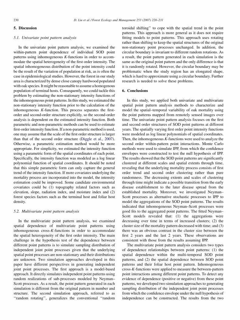
5. Discussion
5.1. Univariate point pattern analysis
In the univariate point pattern analysis, we examined the
within-pattern point dependence of individual SOD point
patterns using inhomogeneous K-functions in order to accom-
modate the spatial heterogeneity of the first order intensity. The
spatial inhomogeneous distribution of the point intensity could
be the result of the variation of population at risk, as is often the
case in epidemiological studies. However, the forest in our study
area is characterized by dense close canopy hardwood populated
with oak species. It might be reasonable to assume a homogenous
population of terminal hosts. Consequently, we could tackle this
problem by estimating the non-stationary intensity functions of
the inhomogeneous point patterns. In this study, we estimated the
non-stationary intensity function prior to the calculation of the
inhomogeneous K-function. This process separates the first-
order and second-order structure explicitly, so the second-order
analysis is dependent on the estimated intensity function. Both
parametric and non-parametric methods can be used to estimate
first-order intensity function. If a non-parametric method is used,
one may assume that the scale of the first order structure is larger
than that of the second order structure (Diggle et al., 2007).
Otherwise, a parametric estimation method would be more
appropriate. For simplicity, we estimated the intensity function
using a parametric form of the spatial coordinates of each point.
Specifically, the intensity function was modeled as a log linear
polynomial function of spatial coordinates. It should be noted
that this simple parametric form can only capture the general
trend of the intensity function. If more covariates underlying the
mortality process are incorporated into the model, the intensity
estimation could be improved. Some candidate environmental
covariates could be (1) topography related factors such as
elevation, slope, radiation index, and moisture index and (2)
forest species factors such as the terminal host and foliar host
density.
5.2. Multivariate point pattern analysis
In the multivariate point pattern analysis, we examined
spatial dependence of multivariate point patterns using
inhomogeneous cross-K-functions in order to accommodate
the spatial heterogeneity of the first order intensity. The main
challenge in the hypothesis test of the dependence between
different point patterns is to simulate sampling distribution of
independent joint point processes given that the underlying
spatial point processes are non-stationary and their distributions
are unknown. Two simulation approaches developed in this
paper have different perspectives in generating independent
joint point processes. The first approach is a model-based
approach. It directly simulates independent point patterns using
random realizations of sub-processes modeled by Neyman–
Scott processes. As a result, the point pattern generated in each
simulation is different from the original pattern in number and
structure. The second simulation approach, referred to as
‘‘random rotating’’, generalizes the conventional ‘‘random
toroidal shifting’’ to cope with the spatial trend in the point
patterns. This approach is more general as it does not require
fitting models to point patterns. This approach uses rotating
rather than shifting to keep the spatial structures of the original
non-stationary point processes unchanged. In addition, the
circular boundary is invariant to different random rotations. As
a result, the point pattern generated in each simulation is the
same as the original point pattern and the only difference is that
it is randomly rotated. However, the circular boundary may be
problematic when the study region has an elongated shape,
which is hard to approximate using a circular boundary. Further
research is needed to solve these problems.
6. Conclusions
In this study, we applied both univariate and multivariate
spatial point pattern analysis methods to characterize and
model the spatial–temporal variability of oak mortality using
the point patterns mapped from remotely sensed images over
time. The univariate point pattern analysis focuses on the first
and second order structures of SOD point patterns at different
years. The spatially varying first order point intensity functions
were modeled as log linear polynomials of spatial coordinates.
Then, the inhomogeneous K-functions were used to analyze the
second order within-pattern point interactions. Monte Carlo
methods were used to simulate IPP, from which the confidence
envelopes were constructed to test the null hypothesis of IPP.
The results showed that the SOD point patterns are significantly
clustered at different scales and spatial extents through time,
revealing that the underlying mortality process consists of first
order trend and second order clustering rather than pure
randomness. The decreasing extents and scales of clustering
through time might indicate a possible transition from the early
disease establishment to the later disease spread from the
established mortality. Moreover, we investigated Neyman–
Scott processes as alternative stochastic processes to IPP to
model the aggregations of the SOD point patterns. The results
indicated that inhomogeneous Neyman–Scott processes were
good fits to the aggregated point patterns. The fitted Neyman–
Scott models revealed that: (1) the aggregations were
decreasing over time in terms of increased clusters; (2) the
cluster size of the mortality pattern decreased with time; and (3)
there was an obvious contrast in the cluster size between the
first 2 years and the last 2 years. These observations are
consistent with those from the results assuming IPP.
The multivariate point pattern analysis considers two types
of dependence relationships between point patterns: (1) the
spatial dependence within the multi-temporal SOD point
patterns, and (2) the spatial dependence between SOD point
patterns and their foliar host point pattern. Inhomogeneous
cross-K-functions were applied to measure the between-pattern
point interactions among different point patterns. To detect any
evidence of dependence (positive or negative) from these point
patterns, we developed two simulation approaches to generating
sampling distribution of the independent joint point processes
from which the confidence envelope under the null hypothesis of
independence can be constructed. The results from the two

D. Liu et al. / Forest Ecology and Management 253 (2007) 220–231 231
approaches were similar and showed that there exist strong
positive dependencies (i.e. attraction) within multi-temporal
SOD point patterns through time, and importantly between SOD
and California bay trees.
Acknowledgements
This work was supported by NASA Headquarters under
the Earth System Science Fellowship Grant NGT5-30493 to
D. Liu. The paper was strengthened with the comments of
anonymous reviewers. The suggestions by Dr. Noel Cressie and
Dr. Adrian Baddeley are appreciated.
References
Arevalo, J.R., Fernandez-Palacios, J.M., 2003. Spatial patterns of trees and
juveniles in a laurel forest of tenerife, canary islands. Plant Ecol. 165, 1–10.
Baddeley, A., Møller, J., Waagepetersen, R., 2000. Non- and semi-parametric
estimation of interaction in inhomogeneous point patterns. Stat. Neerlandica
54, 329–350.
Baddeley, A., Turner, R., 2005. Spatstat: an R package for analyzing spatial
point patterns. J. Stat. Software 12, 1–42.
Batista, J.L.F., Maguire, D.A., 1998. Modeling the spatial structure of tropical
forests. Forest Ecol. Manage. 110, 293–314.
Berndtsson, R., 1989. Topographical and coastal influence of spatial precipita-
tion patterns in tunisia. Int. J. Climatol. 9, 357–369.
Besag, J., 1975. Statistical analysis of non-lattice data. The Statistician 24, 179–
195.
Brodie, C., Houle, G., Fortin, M.J., 1995. Development of a populus balsamifera
clone in subarctic quebec reconstructed from spatial analyses. J. Ecol. 83,
309–320.
Cole, R.G., Syms, C., 1999. Using spatial pattern analysis to distinguish causes
of mortality: an example from kelp in north-eastern New Zealand. J. Ecol.
87, 963–972.
Cressie, N., 1991. Statistics for Spatial Data. Wiley, New York.
Dale, M.R.T., 1999. Spatial Pattern Analysis in Plant Ecology. Cambridge
University Press, Cambridge, United Kingdom.
Davidson, J.M., Wickland, A.C., Patterson, H., Falk, K., Rizzo, D.M., 2005.
Transmission of Phytophthora ramorum in mixed-evergreen forests in
California. Phytopathology 95 (5), 587–596.
Davidson, J.M., Rizzo, D.M., Garbelotto, M., Tjosvold, S., Slaughter, G.W.,
2002. Phytophthora ramorum and sudden oak death is California. II.In:
Transmission and survival, Fifth Symposium on Oak Woodlands, USDA-
Forest Service, San Diego, CA.
Diggle, P.J., 1983. Statistical Analysis of Spatial Point Patterns. Academic
Press, London.
Diggle, P.J., Gomez-Rubio, V., Brown, P.E., Chetwynd, A.G., Gooding, S.,
2007. Second-order analysis of inhomogeneous spatial point processes
using case-control data. Biometrics 63, 550–557.
Franklin, J., Michaelsen, J., Strahler, A.H., 1985. Spatial analysis of density
dependent patterns in coniferous forest stands. Vegetation 64, 29–36.
Goreaud, F., Loreau, M., Millier, C., 2002. Spatial structure and the survival of
an inferior competitor: a theoretical model of neighbourhood competition in
plants. Ecol. Model. 158, 1–19.
Guo, Q., Kelly, M., Gong, P., Liu, D., 2007. An object-based classification
approach in mapping tree mortality using high spatial resolution imagery.
GISci. Remote Sens. 44, 24–47.
Haase, P., 1995. Spatial pattern analysis in ecology based on Ripley’s K-
function: introduction and methods of edge correction. J. Vegetation Sci. 6,
575–582.
Hanisch, K.H., Stoyan, D., 1979. Formulas for second-order analysis of marked
point processes. Math. Operationsforschung Stat. Ser. Stat. 10, 555–560.
Holdenrieder, O., Pautasso, M., Weisberg, P., Lonsdale, D., 2004. Tree diseases
and landscape processes: the challenge of landscape pathology. Trends
Ecol. Evol. 19, 446–452.
Kelly, M., Meentemeyer, R.K., 2002. Landscape dynamics of the spread of
Sudden Oak Death. Photogrammetric Eng. Remote Sens. 68 (10), 1001–
1009.
Kelly, M., Shaari, D., Guo, Q., Liu, D., 2004a. A comparison of standard and
hybrid classifier methods for mapping hardwood mortality in areas affected
by ‘‘sudden oak death’’. Photogrammetric Eng. Remote Sens. 70, 1229–
1239.
Kelly, M., Tuxen, K., Kearns, F., 2004b. Geospatial informatics for management
of a new forest disease: sudden oak death. Photogrammetric Eng. Remote
Sens. 70, 1001–1004.
Liu, D., Kelly, M., Gong, P., 2006. A spatial–temporal approach to monitoring
forest disease spread using multi-temporal high spatial resolution imagery.
Remote Sens. Environ. 101 (2), 167–180.
Lotwick, H.W., Silverman, B.W., 1982. Methods for analyzing spatial processes
of several types of points. J. R. Stat. Soc. B 44, 406–413.
McPherson, B.A., Mori, S.R., Wood, D.L., Storer, A.J., Svihra, P., Kelly, N.M.,
Standiford, R.B., 2005. Sudden oak death in California: disease progression
in oaks and tanoaks. Forest Ecol. Manage. 213, 71–89.
Moeur, M., 1993. Characterizing spatial patterns of trees using stem-mapped
data. Forest Sci. 39 (4), 756–775.
Møller, J., Waagepetersen, R.P., 2004. Statistical Inference and Simulation for
Spatial Point Processes. Chapman and Hall, London.
Penttinen, A., Stoyan, D., Henttonen, H.M., 1992. Marked point process in
forest statistics. Forest Sci. 38 (4), 806–824.
Ristaino, J.B., Gumpertz, M., 2000. New frontiers in the study of dispersal and
spatial analysis of epidemics caused by species in the genus phyophthora.
Annu. Rev. Phytopathol. 38, 541–576.
Rizzo, D., Garbelotto, M., 2003. Sudden oak death: endangering California and
Oregon forest ecosystems. Frontiers Ecol. Environ. 1 (5), 197–204.
Reich, R.M., Lundquist, J.E., 2005. Use of spatial statistics in assessing forest
diseases. pp. 127–143. In: Lundquist, J.E., Hamelin, R.C. (Eds.), Forest
Pathology: From Genes to Landscapes. American Phytopathological
Society Press, St. Paul, MN, 175 pp.
Rizzo, D., Garbelotto, M., Davidson, J.M., Slaughter, G.W., Koike, S.T.,
2002. Phytophthora ramorum as the cause of extensive mortality of
Quercus spp. and Lithocarpus densiflorus in California. Plant Dis. 86
(3), 205–213.
Ripley, B.D., 1977. Modelling spatial patterns. J. R. Stat. Soc. Ser. B 39, 172–
212.
Schurr, F.M., Bossdorf, O., Milton, S.J., Schumacher, J., 2004. Spatial pattern
formation in semi-arid shrubland: a priori predicted versus observed pattern
characteristics. Plant Ecol. 173, 271–282.
Smith, T.E., 2004. A scale-sensitive test of attraction and repulsion between
spatial point patterns. Geogr. Anal. 36 (4), 315–331.
Stoyan, D., Stoyan, H., 1994. Fractals, Random Shapes and Point Field. John
Wiley & Sons Ltd., England.
Suzuki, R.O., Kudoh, H., Kachi, N., 2003. Spatial and temporal variations in
mortality of the biennial plant, Lysimachia rubida: effects of intraspecific
competition and environmental heterogeneity. J. Ecol. 91, 114–125.
Vacek, S., Leps, J., 1996. Spatial dynamics for forest decline: the role of
neighboring trees. J. Vegetation Sci. 7, 789–798.
Waagepetersen, R.P., 2007. An estimation function approach to inference for
inhomogeneous Neyman–Scott processes. Biometrics 63, 252–258.
Welden, C., Slauson, W., Ward, R., 1990. Spatial pattern and interference in
Pinon-Juniper woodlands of northwest Colorado. Great Basin Nat. 50 (4),
313–319.
Wu, X.B., Thurow, T.L., Whisenant, S.G., 2000. Fragmentation and changes in
hydrologic function of tiger bush landscapes, south-west niger. J. Ecol. 88,
790–800.
Wulder, M.A., Hall, R.J., Coops, N.C., Franklin, S.E., 2004. High spatial
resolution remotely sensed data for ecosystem characterization. BioScience
54, 511–521.