FULL PAPER

Charge Neutral Fermionic States and Current Oscillationin a Graphene–Superconductor Hybrid Structure

Wenye Duan, Wei Wang, Chao Zhang, Kuijuan Jin, and Zhongshui Ma

J. Phys. Soc. Jpn. 85, 104713 (2016)

Reprinted from

© 2016 The Physical Society of Japan

Person-to-person distribution by the author only. Not permitted for publication for institutional repositories or on personal Web sites.

Charge Neutral Fermionic States and Current Oscillationin a Graphene–Superconductor Hybrid Structure

Wenye Duan1, Wei Wang1, Chao Zhang2, Kuijuan Jin3,4, and Zhongshui Ma3,4

1School of Physics, Peking University, Beijing 100871, China2School of Physics, University of Wollongong, New South Wales 2522, Australia3Beijing National Laboratory for Condensed Matter Physics, Institute of Physics,

Chinese Academy of Sciences, Beijing 100190, China4Collaborative Innovation Center of Quantum Matter, Beijing 100871, China

(Received May 26, 2016; accepted August 31, 2016; published online September 27, 2016)

The proximity properties of edge currents in the vicinity of the interface between the graphene and superconductor inthe presence of magnetic field are investigated. It is shown that the edge states introduced by Andreev reflection at thegraphene–superconductor (G=S) interface give rise to the charge neutral states in all Landau levels. We note that in atopological insulator–superconductor (TI=S) hybrid structure, only N = 0 Landau level can support this type of chargeneutral states. The different interface states of a G=S hybrid and a TI=S hybrid is due to that graphene consists of twodistinct sublattices. The armchair edge consists of two inequivalent atoms. This gives rise to unique electronic propertiesof edge states when connected to a superconductor. A direct consequence of zero charge states in all Landau levels isthat the current density approaches zero at interface. The proximity effect leads to quantum magnetic oscillation of thecurrent density in the superconductor region. The interface current density can also be tuned with a finite interfacepotential. For sharp δ-type interface potential, the derivative of the wavefunction is discontinuous. As a result, we foundthat there is current density discontinuity at the interface. The step of the current discontinuity is proportional to thestrength of the interface potential.

1. Introduction

A graphene–superconductor (G=S) hybrid structure canexhibit interesting physics not seen in any other systems, e.g.,the specular Andreev reflection (SAR).1,2) Prior to thediscovery of graphene, only the Andreev retro-reflectioncan occur in a normal metal–superconductor (N=S) inter-face.3,4) SAR provides a basis to experimental investigationsof the proximity effect and supercurrent flow in G=S system.So far, most theoretical analysis on the G=S hybrid structureare carried out in absence of a magnetic field.5–8) The edgestates and distribution of edge currents in semi-infinitegraphene under strong magnetic field provide a directevidence of the connection between the edge states andtopological properties of relativistic fermions.9) Under amagnetic field smaller than the critical field of super-conductor, but still large enough, the energy levels of thebulk states are quantized10,11) and the edge states sprawl outat the interface. Under the magnetic field B, the unusualLandau levels (LLs) of graphene have a square-rootdependence on both magnetic field and level indexEN ¼ sgnðNÞ

ffiffiffiffiffiffiffiffiffiffiffiffiffiffiffiffiffiffiffiffiffi2eħv2FjNjB

p, where N is any integer.12) Gen-

erally, the strong magnetic field makes the energy spacingbetween adjacent LLs larger than (or of the same order of)the typical superconducting pair potential (�0 ≲ 1meV). Asa consequence, the magnetic field is expected to affect theAndreev reflection (AR) in G=S junction. Akhmerov andBeenakker propose a method to detect the valley polarizationof quantum Hall edge states, using a superconducting contactas a probe.13,14) In their work the edges are assumed to besmooth on the scale of a magnetic length, lB ¼

ffiffiffiffiffiffiffiffiffiffiffiffiffiħ=jeBj

p, so

that they may be treated locally as a straight line with ahomogeneous boundary condition. For a G=S junction undera strong magnetic field, edge states are formed due to theconfinement introduced by both the external magnetic fieldand the superconducting pair potential. These edge states

produce the Hall current in the direction parallel to theinterface. Physically, these edge states are a coherentsuperposition of electron and hole-like edge excitationssimilar to those realized in finite pn-junction quantum-Hallsamples.14,15)

In this paper, we will demonstrate that the interplay of theAR and skipping cyclotron orbits at the G=S interface givesrise to the charge neutral quasiparticles. Such a charge neutralstate in a topological insulator–superconductor (TI=S) hybridis a topic of intensive current research. Probing zero-modesusing charge transport16) and using quantum Hall edgestates17) have been established. Recently chiral edge stateswith neutral fermions has been observed in synthetic Hallribbons.18) We show a theoretical evidence that the chargeneutral states do exist. Furthermore, in a TI=S hybrid, thecharge neutral quasiparticles only exist in the N ¼ 0 Landaulevel.19) In the present G=S hybrid structure, the chargeneutral quasiparticles can also exist in the high LLs, whichsignificantly enhances the probability of experimentallyobserving the states. Our analysis is based on a hybrid wheregraphene has an armchair edge at the boundary, as shown inFig. 1. The hybrid with a zigzag boundary can be analyzedwith the same method upon a suitable transformation.

Fig. 1. (Color online) Schematic experimental setup with an armchairboundary.

Journal of the Physical Society of Japan 85, 104713 (2016)

http://doi.org/10.7566/JPSJ.85.104713

104713-1 ©2016 The Physical Society of Japan

Person-to-person distribution by the author only. Not permitted for publication for institutional repositories or on personal Web sites.

The paper is organized as follows. In Sect. 2, we discussthe Hamiltonian and formulate the boundary conditions forthe G=S hybrid. In Sect. 3 we analyse the wave-number-dependent excitation spectra and the effective charges ofLandau levels. Section 4 is devoted to the analysis of edgecurrent and Sect. 5 is a brief summary.

2. Hamiltonian and Boundary Conditions

The G=S hybrid with a contact in an armchair configurationis illustrated in Fig. 1, where a uniform magnetic field isapplied in the direction perpendicular to the plane. Weconsider a type-I superconductor in our study so that themagnetic field is absent in the superconductor due to theMeissner effect. For simplicity, we also neglect the effect ofmagnetic penetration to the superconductor and the inhomo-geneity of the magnetic field in the vicinity of the interface.The magnetic field is, then, expressed approximately in form ofBðxÞ ¼ B�ð�xÞ, where �ðxÞ is the Heaviside’s step function.

For honeycomb hexagon lattice with two valley degrees offreedom (K and K0) in the reciprocal space, the Hamiltonianof the system is given as

bH ¼bh � EF � � I4�� � I4 EF � TbhT �1

!; ð1Þ

and the states are described by Dirac–Bogoliubov–de Gennes(DBdG) equation1,20) bH� ¼ E�; ð2Þwhere

bh ¼bhK 0

0 bhK0

!þ UðxÞ þbVðxÞ ð3Þ

is the Dirac Hamiltonian in a form of 4 � 4 matrix acting ontwo inequivalent sublattices and two valley degrees offreedom K and K0, respectively; I4 is a four-dimensionalidentity matrix; Δ is the superconductor pair potential �ðrÞ ¼�0e

i��ðxÞ with �0 the excitation gap and ϕ is the phase of

�ðrÞ in the superconductor; T is the time-reversal operator; Uis the potential UðxÞ ¼ UG�ð�xÞ þ US�ðxÞ which is used tocontrol the difference of Fermi energies in the two regions;bVðxÞ ¼ bV�ðxÞ is a 4 � 4 matrix for the interface potentialwhich describes the barrier effect of an interval insulator layerbetween the graphene and superconductor.

The two inequivalent Dirac cones are given as K ¼ð4�=ð3

ffiffiffi3

paÞ; 0Þ and K0 ¼ ð�4�=ð3

ffiffiffi3

paÞ; 0Þ, where a is the

distance between neighbouring carbon atoms. For the contactof G=S in the armchair configuration, both inequivalentsublattices are on the interface. The wavefunction of DBdGequation can be written in the form

�A ¼ eiKRA AK þ eiK0RA AK0 ; ð4Þ

�B ¼ eiKRB BK þ eiK0RB BK0 ; ð5Þ

where ðA=BÞðK=K0Þ are the components of the spinor ¼ ðu; vÞT, in which u and v ¼ Tu represent electron andhole excitations, respectively. The HamiltonianbhK andbhK0 inthe vicinity of K and K0 points can be derived based on thenearest-neighbor tight-binding model with the k � p methodor with the effective-mass approximation.21,22) Near the Diraccones, bhK and bhK0 are found as

bhK ¼ vFð�x�x þ �y�yÞ ¼ vF0 �x � i�y

�x þ i�y 0

!ð6Þ

and bhK0 ¼ vFð��x�x þ �y�yÞ

¼ vF0 ��x � i�y

��x þ i�y 0

!; ð7Þ

where � ¼ p þ eA and vF ¼ vGF�ð�xÞ þ vSF�ðxÞ, vDF and vSFare the Fermi velocities in the graphene and superconductor.The time reversal operator in Eq. (1) takes the form T ¼ð 0 I2�2I2�2 0

ÞC ¼ T �1 with C the operator of complex conjuga-tion. According to the Hamiltonian, the wave function can bewritten as,

� ¼ ðeÞAK; ðeÞ

BK; ðeÞAK0 ; ðeÞ

BK0 ; ðhÞAK0 ; ðhÞ

BK0 ; ðhÞAK; ðhÞ

BK

� �T;

where T stands for transpose. Because both inequivalentsublattices are on the interface for the armchair configuration,the interface potential is presented by delta potentialsVAKðrÞ ¼ V0�ðx ¼ 0Þ, VBKðrÞ ¼ V0�ðx ¼ 0Þ, VAK0 ðrÞ ¼V0�ðx ¼ 0Þ, and VBK0 ðrÞ ¼ V0�ðx ¼ 0Þ for the atoms at Aand B sublattices. Employing the wavefunctions given inEqs. (4) and (5), the interfance potential in the basis ðeÞA=B;K=K0 , ðhÞ

A=B;K=K0 is given as

V̂ ¼ V0

I2�2 I2�2

I2�2 I2�2

!: ð8Þ

For convenient calculations, we introduce an unitarytransformation,

� ¼�4�4 0

0 �4�4

!ð9Þ

with

�4�4 ¼I2�2 0

0 �z

!: ð10Þ

Under this unitary transformation, the Hamiltonian in Eq. (1)becomes,

cH0 ¼ �bH�y ¼bh0 � EF � � I4�� � I4 EF � T 0bh0T 0�1

!; ð11Þ

where

bh0 ¼ bh0K 0

0 bh0K0

!þUðxÞ þ bV0ðxÞ ð12Þ

and

bV0 ¼ �4�4bV�y4�4 ¼ V0

I2�2 �z

�z I2�2

!ð13Þ

with bh0K ¼ vFð�x�x þ �y�yÞ; ð14Þbh0K0 ¼ vFð�x�x � �y�yÞ: ð15Þ

Here we notice that T 0bV0T 0�1 ¼ bV0. Correspondingly, thewavefunction is given by e� ¼ �4�4�, i.e.,

J. Phys. Soc. Jpn. 85, 104713 (2016) W. Duan et al.

104713-2 ©2016 The Physical Society of Japan

Person-to-person distribution by the author only. Not permitted for publication for institutional repositories or on personal Web sites.

e� ¼ ðeÞAK; ðeÞ

BK; ðeÞAK0 ; � ðeÞ

BK0 ; ðhÞAK0 ; ðhÞ

BK0 ; ðhÞAK; � ðhÞ

BK

� �T:

In the spinor representation ¼ ðu; vÞT, it corresponds to a transformed forme� ¼ euAK; euBK; euAK0 ; euBK0 ; evAK0 ; evBK0 ; evAK; evBK� �T:

To obtain the boundary conditions for the electron andhole excitations, we integrate DBdG equation cross over theinterface. Due to the features of a delta-type of interfacepotential and first order differential equation of DBdG, thewavefunctions are discontinuous crossing the interfacebetween the graphene and superconductor. Consequently,the particle-like and hole-like components require to satisfyfollowing boundary conditionseuAKð0þÞ þeuAK0 ð0þÞ ¼euAKð0�Þ þeuAK0 ð0�Þ;evAKð0þÞ þevAK0 ð0þÞ ¼evAKð0�Þ þevAK0 ð0�Þ;euBKð0þÞ �euBK0 ð0þÞ ¼euBKð0�Þ �euBK0 ð0�Þ;evBKð0þÞ �evBK0 ð0þÞ ¼evBKð0�Þ �evBK0 ð0�Þ;euAKð0þÞ �euAKð0�Þ ¼ �ieV0½euBKð0Þ �euBK0 ð0Þ�;evAK0 ð0þÞ �evAK0 ð0�Þ ¼ �ieV0½�evBKð0Þ þevBK0 ð0Þ�;euBKð0þÞ �euBKð0�Þ ¼ �ieV0½euAKð0Þ þeuAK0 ð0Þ�;evBK0 ð0þÞ �evBK0 ð0�Þ ¼ �ieV0½evAKð0Þ þevAK0 ð0Þ�; ð16Þ

where eV0 ¼ V0=2ħððvGF Þ�1 þ ðvSFÞ�1Þ. This implies that theboundary conditions manifest a linear combination of statesfrom two valleys in the armchair configuration. This stemsfrom that fact that both inequivalent sublattices appear at theinterface. For simplify, we will omit the wavy line above thewavefunction from now on.

3. Energy Spectra and Effective Charges

3.1 Wavefunctions in the graphene and superconductorregions

The eigenstates in graphene and superconductor can beobtained by solving the DBdG equations in these two regionsseparately. We assume that the excitation gap is real andisotropic, �ðrÞ ¼ �0�ðxÞ, in both the sublattice and the valleydegrees of freedom. In addition, the energies of chargecarriers in graphene is restricted in a window jEj � �0, sothat electron and hole excitations with jEj � �0 are confinedon the graphene side in a width of a magnetic length lB in thevicinity of interface by the magnetic field. For a magneticfield perpendicular to the graphene sheet, B ¼ ð0; 0; BÞ, thevector potential is given as A ¼ ð0; Bx; 0Þ�ð�xÞ.

The eigenvalues of the DBdG equation in the region of agraphene (x < 0) are found as En;�� ¼ ��

ffiffiffiffiffiffi2n

pþ ð�1Þ�EF,

where n is any positive integer, � ¼ 1; 2 indicate theelectrons and holes, respectively, and �� ¼ �1 representthe solutions for the conduction band and the valence band.Based on the eigenstates the wavefunction for the energy E(i.e., z) and the wavevector ky in the graphene side can bewritten as

�G�;ðx; y; ky; zÞ ¼

1ffiffiffiffiffiLy

p eikyy�G�;ðx; ky; zÞ ð17Þ

with

�G�þ;þðx; ky; zþÞ ¼ i

ffiffiffiffiffizþ

pDzþ�1ð�

ffiffiffi2

pðx þ kyÞÞ; Dzþð�

ffiffiffi2

pðx þ kyÞÞ; 0; 0; 0; 0; 0; 0

� �T;

�G��;þðx; ky; zþÞ ¼ 0; 0; Dzþð�

ffiffiffi2

pðx þ kyÞÞ; i

ffiffiz

pDzþ�1ð�

ffiffiffi2

pðx þ kyÞÞ; 0; 0; 0; 0

� �T;

�G��;�ðx; ky; z�Þ ¼ 0; 0; 0; 0; Dz�ð�

ffiffiffi2

pðx � kyÞÞ; �i ffiffiffiffiffi

z�p

Dz��1ð�ffiffiffi2

pðx � kyÞÞ; 0; 0

� �T;

�G�þ;�ðx; ky; z�Þ ¼ 0; 0; 0; 0; 0; 0; �i ffiffiffiffiffi

z�p

Dz��1ð�ffiffiffi2

pðx � kyÞÞ; Dz�ð�

ffiffiffi2

pðx � kyÞÞ

� �T; ð18Þ

where z ¼ ðE þ EFÞ2=2 is parameter to be obtained self-consistently from the boundary conditions, and DzðxÞ is a paraboliccylinder function. � ¼ �1 for the pseudospin A (+) and B (−) subspaces, ¼ �1 for the K (+) and K0 (−) valleys, and ¼ �1for electrons (+) and holes (−), respectively. Here, we use the unit where the length is scaled by lB and the energy is scaled byE0 ¼ ħvGF =lB, respectively. We also define the guiding-center coordinates Xky ¼ �kyl2B and �Xky for the cyclotron motion ofelectrons and holes in the normal region.

In the same way, the eigenvalues of the DBdG equation in the superconductor side are found as E�� ¼�

ffiffiffiffiffiffiffiffiffiffiffiffiffiffiffiffiffiffiffiffiffiffiffiffiffiffiffiffiffiffiffiffiffiffiffiffiffiffiffiffiffiffiffiffiffiffiffiffiffiffiffiffiffiffiffiffiffiffiffi½U0 þ EF þ �ðvSF=vGF Þk�2 þ�2

0

p, where � ¼ �1 for the electron and hole bands, respectively, � ¼ �1 and k ¼

ffiffiffiffiffiffiffiffiffiffiffiffiffiffik2x þ k2y

p.

The wavefunction for the energy E and the wavevector ky in the superconductor side can be written as,

�S�;ðx; y; ky; EÞ ¼

1ffiffiffiffiffiLy

p e�ikðÞx xþikyy�S�

;ðky; EÞ; ð19Þ

with

�S�þ;ðky; EÞ ¼ exp i

� þ �

2

� ��kðÞx � iky

kexp i

� þ �

2

� �; 0; 0; exp �i� þ �

2

� ��kðÞx � iky

k; exp �i� þ �

2

� �; 0; 0

� �T

;

�S��;ðky; EÞ ¼ 0; 0; exp i

� þ �

2

� ��kðÞx þ iky

kexp i

� þ �

2

� �; 0; 0; exp �i� þ �

2

� ��kðÞx þ iky

k; exp �i� þ �

2

� �� �T

; ð20Þ

where the meaning of κ and λ are defined as those for the graphene, � ¼ tan�1ffiffiffiffiffiffiffiffiffiffiffiffiffiffiffiffiffiffiffiffiffiffiffiffiffið�0=EÞ2 � 1

p. kðÞx ¼ k0 þ ik00 with

k0 ¼ sign½U0 þ EF�ðvGF =vSFÞffiffiffiffiffiffiffiffiffiffiffiffiffiffiffiffiffiffiffiffiffiffiffiffiffiffiffiffiffiffiffiffiffiffiffiffiffiffiðjU0 þ EFjÞð� þ Þ

p, k00 ¼ ðvGF =vSFÞ

ffiffiffiffiffiffiffiffiffiffiffiffiffiffiffiffiffiffiffiffiffiffiffiffiffiffiffiffiffiffiffiffiffiffiffiffiffiffiðjU0 þ EFjÞð � �Þ

p, � ¼ ½ðU0 þ EFÞ2 ��2

0 þ E2 �ðvSF=vGF Þ2k2y�=½2jU0 þ EFj�, and ¼

ffiffiffiffiffiffiffiffiffiffiffiffiffiffiffiffiffiffiffiffiffiffiffiffiffiffiffi�2

0 � E2 þ �2p

.

J. Phys. Soc. Jpn. 85, 104713 (2016) W. Duan et al.

104713-3 ©2016 The Physical Society of Japan

Person-to-person distribution by the author only. Not permitted for publication for institutional repositories or on personal Web sites.

Using �G�;ðx; y; ky; EÞ and �S�

;ðx; y; ky; EÞ, the wavefunc-tions in the graphene and superconductor regions canthen be expressed in the form �Nðx; y; ky; EÞ ¼P

;;� c�;�

G�;ðx; y; ky; EÞ and �Sðx; y; ky; EÞ ¼P

;;� d�;�

S�;ðx; y; ky; EÞ, respectively. The coefficients c�;

and d�; can be determined by the boundary conditions. For�G�; those with � ¼ þ1 are divergent when x ! �1, so

cþ; ¼ 0. Similarly, d�; ¼ 0. In general, the boundaryconditions yield an homogeneous linearity equation of c�;and d�;. We can found the energy spectrum from thecondition for existing nonzero solution. The remainingcoefficient (for example c�þ;þ) can be decided by thenormalization condition

Rþ1�1

RLydx�yðx; yÞ�ðx; yÞ ¼ 1, i.e.,

1 ¼X

¼�;¼�jc�;j2

Z 0

�1dxfD2

zð�

ffiffiffi2

pðx þ kyÞÞ

þ zD2z�1ð�

ffiffiffi2

pðx þ kyÞÞg

þX¼�

ðjdþ;þj2 þ jdþ;�j2Þ1

k00kþx � iky

kþ

���� ����2 þ 1

!

þ 2X¼�

Re�idþ�þd

þ�

E

�0k�x

� kþx � ikykþ

� ��k�x � iky

k�þ 1

�: ð21Þ

After performing these procedures, we can obtain the energyspectrum and wavefunctions for whole region.

3.2 Xky -dependence of energy spectrum ENðXkyÞBy including a delta-function potential of strength V0 at

the interface, the contact of graphene and superconductorcan be regarded as a metallic contact for V0 ¼ 0 and atunneling junction for a finite value of V0. The Xky -dependence of ENðXkyÞ manifests the existence of edgestates. The dispersion of edge states is sensitive to both theFermi energy EF and the strength of the interface potentialV0.

In this work our purpose is to demonstrate that for astrongly coupled G=S system, charge neutral Fermionic statescan exist in all LLs. The necessary conditions for strong G=Scoupling and charge neutral states in high LLs are a near zeroFermi energy and a small superconductor pair potential. Fortypical s-wave superconductors, the pair potential is verysmall �0=E0 1. There is a significant difference betweenthe energy spectra for large �0 and small �0. We firstexamine the spectra with a large (unrealistic) �0=E0 1.This situation was previously studied in Ref. 13. The inset ofFig. 2 shows the energy spectra for �0=E0 ¼ 10 under twodifferent interface potentials, V0 ¼ 0 and V0 ¼ 10000 (allenergies are in unit of E0). For V0 ¼ 0, there is a valleydegeneracy. The left side is for the electron-like particleswhile right side is for the hole-like particles. For non-zerointerface potential V0 ¼ 10000 the valley degenerate is liftedand energy levels are split in the region of the intermediatevalues of Xky . In general, the splitting enlarges as the V0

increases. The AR induced mixing between electron- andhole-like levels becomes weaker with V0 increasing, or thenormal reflection turns to stronger. For larger jXky j theselevels trend to the same asymptotic degenerate levels. So thedelta potential strength V0 could tune the proportion of the

AR at the boundary. The Xky -dependent energy spectrum hasthe symmetry ENðXkyÞ ¼ �E�Nð�XkyÞ.

The interplay of cyclotron motion in the graphene regionand the AR from the interface with the superconductor regionresults in the formation of chiral Dirac–Andreev edge stateswith guiding-center-dependent electric charge19) for jEj <�0. These solutions can be described as interface states in thesense that they are localized electron states in the directionperpendicular to the interface and propagate along theinterfaces, in analogy to the edge states of a semi-infinitegraphene in a magnetic field. In contrast with conventionaledge states, the V0 ¼ 0 interface does not cause splitting ofthe dispersion. This is a consequence that at the G=S interfacewith V0 ¼ 0, the wave function is finite and continuousand the associated probability density can be finite in thesuperconductor region.

We found that for a small (more realistic) Δ and EF ¼ 0

(for AR to dominate) G=S coupling becomes very strong andqualitatively alters the energy dispersion. Figure 2 shows theclear and convincing evidence of the G=S coupling of thehybrid. For EF ¼ 0 the reflection is in the SAR regime. For alarge superconductor pair potential, the G=S coupling is veryweak. Therefore the energy levels are approximately theLandau levels of graphene. This is shown with blue curves.For a small superconductor pair potential, the coupling of thegraphene with the superconductor results in a decrease of theenergy levels. The coupling is stronger where the carrierdensity is higher in the graphene. Since the density of aLandau level varies with Xky , the energy becomes dispersivewith Xky . For N ¼ 1, the carrier concentration peaks atXky ¼ 0 and thus the energy minimum occurs at Xky ¼ 0. ForN ¼ 2 the carrier concentration has two peaks at finite Xkyand the energy dispersion has two minima at finite Xky . Forthe Nth Landau level, there are N concentration maxima. Thenumber of energy minima equals the number of concentrationmaxima.

3.3 Effective electrical charge of the single-particleexcitations

As in the case for Bogoliubov quasiparticles in aconventional superconductor, the Dirac–Andreev edge states

Fig. 2. (Color online) The energy dispersion for EF ¼ 0, the red dash lineis for the pair potential �0 ¼ 2:5 and the blue line is for �0 ¼ 10. Inset:Energy dispersion relation ENðXky Þ for Fermi energy EF ¼ 1 and the pairpotential �0 ¼ 10. The blue line is for V0 ¼ 0. The red lines represent the Kand KA valleys, respectively, for V0 ¼ 10000.

J. Phys. Soc. Jpn. 85, 104713 (2016) W. Duan et al.

104713-4 ©2016 The Physical Society of Japan

Person-to-person distribution by the author only. Not permitted for publication for institutional repositories or on personal Web sites.

are coherent superpositions of particles and holes. Con-sequently, their effective electrical charge generally has anonquantized value and is given by

eð�Þ ¼Zd2r½�ðrÞ�yz�ðrÞ; ð22Þ

where z ¼ ð I4 0

0 �I4Þ.

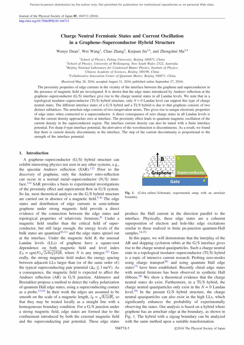
The calculated effective charges eðN;Xky Þ of states �NðXkyÞfor N ¼ 0, 1, 2, 3 with V0 ¼ 0 are shown in Fig. 3 as afunction of Xky . The effective charge changes the sign, whichindicates the presence of a neutral Fermionic mode at a finitevalue of Xky . The neutral Fermionic mode has beendemonstrated recently in a TI=S hybrid.19) The mechanismand properties of the neutral Fermionic states presented herefor the G=S hybrid are quite different to that in a TI=S hybrid.The neutral Fermionic state in a G=S hybrid is due to thecoupling between orbital motion and the pseudo spin. Themathematical structure of the Hamiltonian is very similarfor both systems. For N ¼ 0 mode, eð0;�Xky Þ ¼ �eð0;Xky Þ. TheN ¼ 0 state has zero effective charge at Xky ¼ 0. The moreremarkable picture here is that, for a zero Fermi level, theneutral Fermionic state can also exist in higher Landau levels,i.e., eð�N;�Xky Þ ¼ �eðN;Xky Þ. This results in a zero effectivechange at Xky ¼ 0 for N ≠ 0. This effect is totally missing ina TI=S hybrid. The result is a direct consequence of DBdGequation. As mentioned early the definition of the effectivecharge given by Eq. (5) is not a quantum number and it ispossible for it to acquire any value. For the N ¼ 0 LL, the

charge neutral state has a unique property that its antiparticleis itself. For the charge neutral states in high LLs, thisrequirement is not satisfied. In the present system, thesymmetry eðN;�Xky Þ ¼ �eðN;Xky Þ is maintained but clearly theantiparticle of the charge neutral state in the Nth LL is notitself. We note that the effective charge in the high LL canalso acquire a zero value in a TI=S hybrid.19) However, in theTI=G hybrid it occurs at finite wavenumbers and does nothave the symmetry of eðN;�Xky Þ ¼ �eðN;Xky Þ. This symmetry inthe G=S hybrid is a direct consequence of valley degeneracyin the graphene and the Andreev reflection at the interface.Formation of charge neutral states is of importance inunderstanding the nature of the interface states in a G=Shybrid. At the G=S interface, an incident electron in the K-valley can only pair with another electron in the KA-valley.

Although the charge neutral Fermionic states reported herehave the property of eðN;0Þ ¼ 0, they are not strictly Majoronamode. Such non-Majorona charge neutral modes can result ininteresting physical properties. For example, a totally differ-ent type of charge neutral Fermionic modes have beenproposed and detected in fractional quantum Hall states.23,24)

These modes played an important role in understanding thefractional quantum Hall states of ¼ 8=3; 7=3. Recentlychiral edge states with neutral fermions has been observed insynthetic Hall ribbons.18)

A solution of electronic state being electrically neutral isnot only important conceptually in understanding why theybehave as they do, it is also useful in the quantitativeanalysis, because it provides a link between the concen-trations of the incident electrons and the reflected holes. Amost important consequence of this principle is that it is notpossible to add a single species of electron to a solution all byitself. Some other species of opposite charge (reflection hole)must always be added at the same time, and its amount andidentity must be incorporated into calculations of effectivecharge.

4. Edge Current in the Vicinity of G=S Interface

4.1 Formulation of charge current densityThe edge states can produce the current in the vicinity of

both sides of interface. Starting from the time-dependentversion of the DBdG Eq. (1)

iħ@

@t� ¼ bH� ð23Þ

with the wave function:

� ¼ uAK; uBK; uAK0 ; uBK0 ; vAK0 ; vBK0 ; vAK; vBK� �T

¼ uK; uK0 ; vK0 ; vK� �T ¼ u; v

� �T; ð24Þ

the following continuity equation for the probability current

@t�u

�

!þ @y

Ju

J

!¼

S

�S

!ð25Þ

are got, where

S ¼ 2Imð�uyvÞħ

: ð26Þ

Specific to the NS graphene junction described in this paper,the current flows in y-direction. So, we look at the currents

near the interface where for each quasiparticle state M ¼½Xky ; EðXkyÞ� in the spectrum the electron-like and hole-likeexcitations probability currents density25) JuM and JvM are

JuM ¼ vF½uyK�yuK � uyK0�yuK0 � ð27Þand

JvM ¼ �vF½vyK�yvK � vyK0�yvK0 �: ð28ÞSum over all quasiparticle states and the charge currentdensity at the interface is found as

Fig. 3. (Color online) Effective electric charge eðN;Xky Þ of the single-particle excitations as a function of Xky (in units of lB) for N ¼ 0; 1; 2; 3

Landau branches as shown in the legend. The delta potential strength isV0 ¼ 0 and �0 ¼ 2:5.

J. Phys. Soc. Jpn. 85, 104713 (2016) W. Duan et al.

104713-5 ©2016 The Physical Society of Japan

Person-to-person distribution by the author only. Not permitted for publication for institutional repositories or on personal Web sites.

J ¼ eXM

ð fMJuM þ ð1 � fMÞJvMÞ

¼ evFXM

ð fMðuyK�yuK � uyK0�yuK0 Þ

� ð1 � fMÞðvyK�yvK � vyK0�yvK0 ÞÞ

¼ evFXM

ð fMðuyK�yuK � uyK0�yuK0 þ vyK�yvK � vyK0�yvK0 Þ

� ðvyK�yvK � vyK0�yvK0 ÞÞ; ð29Þwhere fM ¼ f0ðE � �EFÞ, f0ðEÞ ¼ 1

e�Eþ1 is the Fermi–Diracdistribution, EF is the Fermi energy at the superconductivityregion, and � ¼ 1 (−1) for the electron (hole) component.The formulation for the current of BdG equation is defined inRef. 26 by written in terms of a sum over quasiparticle states,J ¼ JBdG þ JVAC where the BdG quasiparticle component ofthe electron current is given by the term linear in ffMg and onthe other hand, the condensate vacuum current is identifiedwith the term which is independent of the occupationprobabilities f fMg, i.e.,

JBdG ¼ eXM

½JuM � JvM� fM ð30Þ

and

JVAC ¼ eXM

JvM: ð31Þ

All the states below the Fermi energy can contribute to thecurrent. Taking account all the states, the spatial distributionsof charge currents can written in the form

JL ¼Zdky

XEðXky Þ

fFðEÞðjc�þþj2 þ jc��þj2Þ

ðE þ EFÞffiffiffi2

p

�Dzþ�1ð�ffiffiffi2

pðx þ kyÞÞDzþð�

ffiffiffi2

pðx þ kyÞÞ

� ð1 � fFðEÞÞðjc�þ�j2 þ jc���j2ÞðE � EFÞ=ffiffiffi2

pDz��1

� ð�ffiffiffi2

pðx � kyÞÞDz�ð�

ffiffiffi2

pðx � kyÞÞ

ð32Þ

in the graphene region and

JR ¼ vSFvGF

XEðkyÞ

Zdky e

�2k00x2X¼�

(ð fFðEÞ � 1Þðjdþþj2

þ jdþ�j2Þ ImkðþÞx � iky

kþ

� �þ fFðEÞ2 cos � Im dþþd

þ��e

2ik0x ðkðþÞx � ikyÞkþ

� 2 Im dþþdþ��e

2ik0xe�i�ðkðþÞx � ikyÞ

kþ

)ð33Þ

in the superconductor region.

4.2 Distribution of equilibrium edge currentBecause we are interested in those contributions due to the

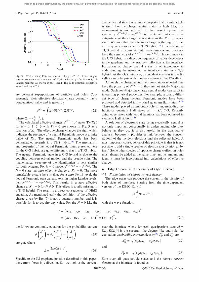
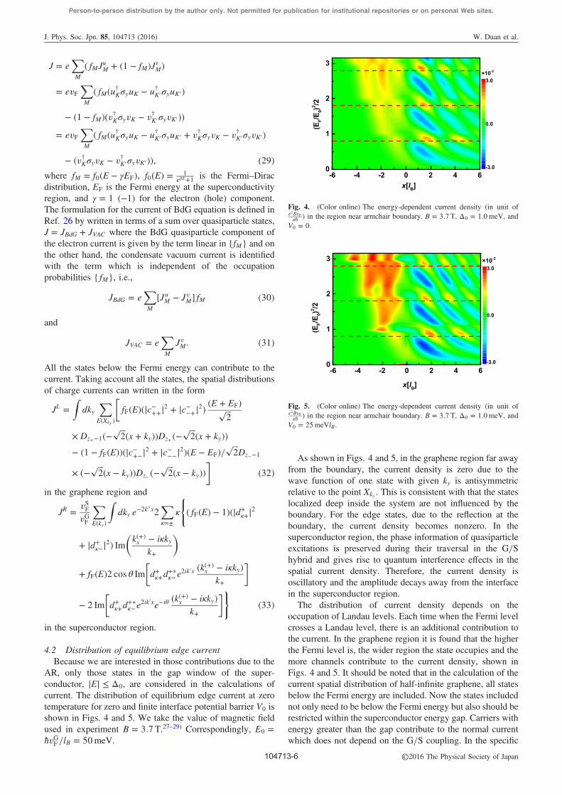
AR, only those states in the gap window of the super-conductor, jEj � �0, are considered in the calculations ofcurrent. The distribution of equilibrium edge current at zerotemperature for zero and finite interface potential barrier V0 isshown in Figs. 4 and 5. We take the value of magnetic fieldused in experiment B ¼ 3:7T.27–29) Correspondingly, E0 ¼ħvGF =lB ¼ 50meV.

As shown in Figs. 4 and 5, in the graphene region far awayfrom the boundary, the current density is zero due to thewave function of one state with given ky is antisymmetricrelative to the point Xky . This is consistent with that the stateslocalized deep inside the system are not influenced by theboundary. For the edge states, due to the reflection at theboundary, the current density becomes nonzero. In thesuperconductor region, the phase information of quasiparticleexcitations is preserved during their traversal in the G=Shybrid and gives rise to quantum interference effects in thespatial current density. Therefore, the current density isoscillatory and the amplitude decays away from the interfacein the superconductor region.

The distribution of current density depends on theoccupation of Landau levels. Each time when the Fermi levelcrosses a Landau level, there is an additional contribution tothe current. In the graphene region it is found that the higherthe Fermi level is, the wider region the state occupies and themore channels contribute to the current density, shown inFigs. 4 and 5. It should be noted that in the calculation of thecurrent spatial distribution of half-infinite graphene, all statesbelow the Fermi energy are included. Now the states includednot only need to be below the Fermi energy but also should berestricted within the superconductor energy gap. Carriers withenergy greater than the gap contribute to the normal currentwhich does not depend on the G=S coupling. In the specific

Fig. 4. (Color online) The energy-dependent current density (in unit ofe2BvF�ħ ) in the region near armchair boundary. B ¼ 3:7T, �0 ¼ 1:0meV, andV0 ¼ 0.

Fig. 5. (Color online) The energy-dependent current density (in unit ofe2BvF�ħ ) in the region near armchair boundary. B ¼ 3:7T, �0 ¼ 1:0meV, andV0 ¼ 25meVlB.

J. Phys. Soc. Jpn. 85, 104713 (2016) W. Duan et al.

104713-6 ©2016 The Physical Society of Japan

Person-to-person distribution by the author only. Not permitted for publication for institutional repositories or on personal Web sites.

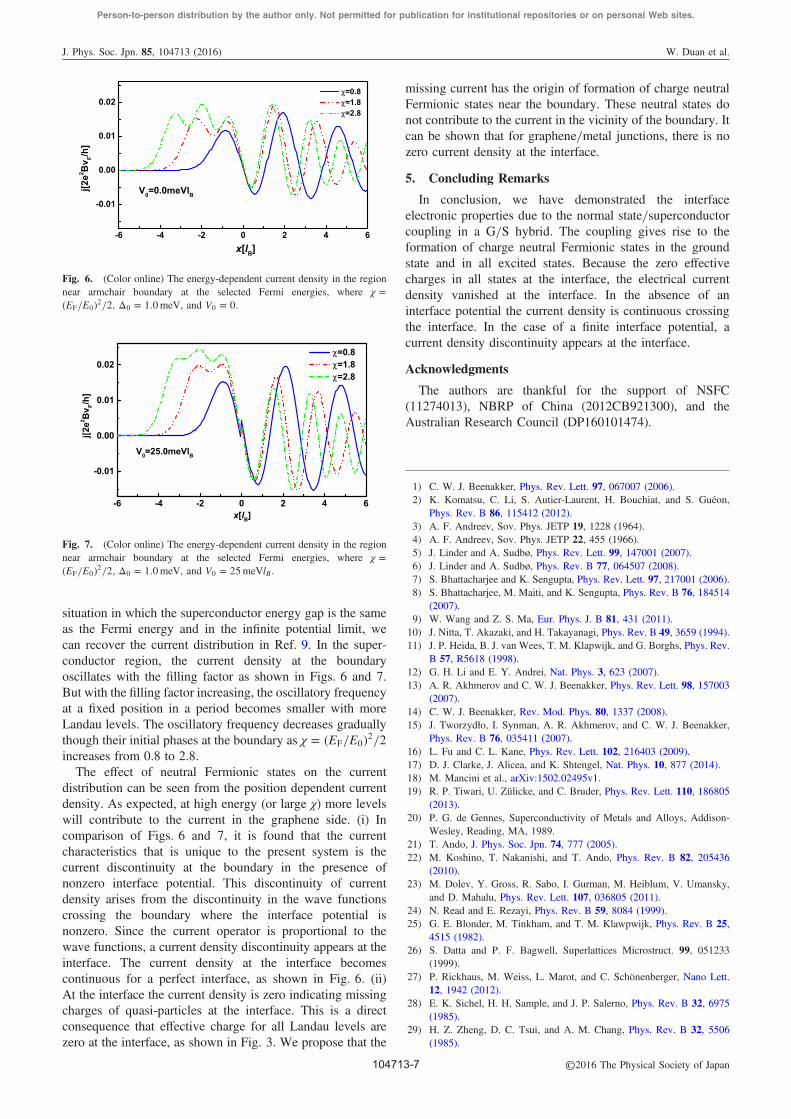
situation in which the superconductor energy gap is the sameas the Fermi energy and in the infinite potential limit, wecan recover the current distribution in Ref. 9. In the super-conductor region, the current density at the boundaryoscillates with the filling factor as shown in Figs. 6 and 7.But with the filling factor increasing, the oscillatory frequencyat a fixed position in a period becomes smaller with moreLandau levels. The oscillatory frequency decreases graduallythough their initial phases at the boundary as � ¼ ðEF=E0Þ2=2increases from 0.8 to 2.8.

The effect of neutral Fermionic states on the currentdistribution can be seen from the position dependent currentdensity. As expected, at high energy (or large χ) more levelswill contribute to the current in the graphene side. (i) Incomparison of Figs. 6 and 7, it is found that the currentcharacteristics that is unique to the present system is thecurrent discontinuity at the boundary in the presence ofnonzero interface potential. This discontinuity of currentdensity arises from the discontinuity in the wave functionscrossing the boundary where the interface potential isnonzero. Since the current operator is proportional to thewave functions, a current density discontinuity appears at theinterface. The current density at the interface becomescontinuous for a perfect interface, as shown in Fig. 6. (ii)At the interface the current density is zero indicating missingcharges of quasi-particles at the interface. This is a directconsequence that effective charge for all Landau levels arezero at the interface, as shown in Fig. 3. We propose that the

missing current has the origin of formation of charge neutralFermionic states near the boundary. These neutral states donot contribute to the current in the vicinity of the boundary. Itcan be shown that for graphene=metal junctions, there is nozero current density at the interface.

5. Concluding Remarks

In conclusion, we have demonstrated the interfaceelectronic properties due to the normal state=superconductorcoupling in a G=S hybrid. The coupling gives rise to theformation of charge neutral Fermionic states in the groundstate and in all excited states. Because the zero effectivecharges in all states at the interface, the electrical currentdensity vanished at the interface. In the absence of aninterface potential the current density is continuous crossingthe interface. In the case of a finite interface potential, acurrent density discontinuity appears at the interface.

Acknowledgments

The authors are thankful for the support of NSFC(11274013), NBRP of China (2012CB921300), and theAustralian Research Council (DP160101474).

1) C. W. J. Beenakker, Phys. Rev. Lett. 97, 067007 (2006).2) K. Komatsu, C. Li, S. Autier-Laurent, H. Bouchiat, and S. Guéon,

Phys. Rev. B 86, 115412 (2012).3) A. F. Andreev, Sov. Phys. JETP 19, 1228 (1964).4) A. F. Andreev, Sov. Phys. JETP 22, 455 (1966).5) J. Linder and A. Sudbø, Phys. Rev. Lett. 99, 147001 (2007).6) J. Linder and A. Sudbø, Phys. Rev. B 77, 064507 (2008).7) S. Bhattacharjee and K. Sengupta, Phys. Rev. Lett. 97, 217001 (2006).8) S. Bhattacharjee, M. Maiti, and K. Sengupta, Phys. Rev. B 76, 184514

(2007).9) W. Wang and Z. S. Ma, Eur. Phys. J. B 81, 431 (2011).10) J. Nitta, T. Akazaki, and H. Takayanagi, Phys. Rev. B 49, 3659 (1994).11) J. P. Heida, B. J. van Wees, T. M. Klapwijk, and G. Borghs, Phys. Rev.

B 57, R5618 (1998).12) G. H. Li and E. Y. Andrei, Nat. Phys. 3, 623 (2007).13) A. R. Akhmerov and C. W. J. Beenakker, Phys. Rev. Lett. 98, 157003

(2007).14) C. W. J. Beenakker, Rev. Mod. Phys. 80, 1337 (2008).15) J. Tworzydło, I. Synman, A. R. Akhmerov, and C. W. J. Beenakker,

Phys. Rev. B 76, 035411 (2007).16) L. Fu and C. L. Kane, Phys. Rev. Lett. 102, 216403 (2009).17) D. J. Clarke, J. Alicea, and K. Shtengel, Nat. Phys. 10, 877 (2014).18) M. Mancini et al., arXiv:1502.02495v1.19) R. P. Tiwari, U. Zülicke, and C. Bruder, Phys. Rev. Lett. 110, 186805

(2013).20) P. G. de Gennes, Superconductivity of Metals and Alloys, Addison-

Wesley, Reading, MA, 1989.21) T. Ando, J. Phys. Soc. Jpn. 74, 777 (2005).22) M. Koshino, T. Nakanishi, and T. Ando, Phys. Rev. B 82, 205436

(2010).23) M. Dolev, Y. Gross, R. Sabo, I. Gurman, M. Heiblum, V. Umansky,

and D. Mahalu, Phys. Rev. Lett. 107, 036805 (2011).24) N. Read and E. Rezayi, Phys. Rev. B 59, 8084 (1999).25) G. E. Blonder, M. Tinkham, and T. M. Klawpwijk, Phys. Rev. B 25,

4515 (1982).26) S. Datta and P. F. Bagwell, Superlattices Microstruct. 99, 051233

(1999).27) P. Rickhaus, M. Weiss, L. Marot, and C. Schönenberger, Nano Lett.

12, 1942 (2012).28) E. K. Sichel, H. H. Sample, and J. P. Salerno, Phys. Rev. B 32, 6975

(1985).29) H. Z. Zheng, D. C. Tsui, and A. M. Chang, Phys. Rev. B 32, 5506

(1985).

Fig. 7. (Color online) The energy-dependent current density in the regionnear armchair boundary at the selected Fermi energies, where � ¼ðEF=E0Þ2=2, �0 ¼ 1:0meV, and V0 ¼ 25meVlB.

Fig. 6. (Color online) The energy-dependent current density in the regionnear armchair boundary at the selected Fermi energies, where � ¼ðEF=E0Þ2=2, �0 ¼ 1:0meV, and V0 ¼ 0.

J. Phys. Soc. Jpn. 85, 104713 (2016) W. Duan et al.

104713-7 ©2016 The Physical Society of Japan