Embed Size (px)
Citation preview
doi.org/10.26434/chemrxiv.11294480.v1
ChemEnv : A Fast and Robust Coordination Environment IdentificationToolDavid Waroquiers, Janine George, Matthew Horton, Stephan Schenk, Kristin Persson, Gian-MarcoRignanese, Xavier Gonze, Geoffroy Hautier
Submitted date: 28/11/2019 • Posted date: 17/12/2019Licence: CC BY-NC-ND 4.0Citation information: Waroquiers, David; George, Janine; Horton, Matthew; Schenk, Stephan; Persson,Kristin; Rignanese, Gian-Marco; et al. (2019): ChemEnv : A Fast and Robust Coordination EnvironmentIdentification Tool. ChemRxiv. Preprint. https://doi.org/10.26434/chemrxiv.11294480.v1
Coordination or local environments have been used to describe, analyze, and understand crystal structuresfor more than a century. Here, we present a new tool called ChemEnv, which can identify coordinationenvironments in a fast and robust manner. In contrast to previous tools, the assessment of the coordinationenvironments is not biased by small distortions of the crystal structure. Its robust and fast implementationenables the analysis of large databases of structures. The code is available open source within the pymatgenpackage and the software can as well be used through a web app available on http://crystaltoolkit.org throughthe Materials Project.
File list (2)
download fileview on ChemRxivpaper.pdf (4.27 MiB)
download fileview on ChemRxivsupplementary_information.pdf (159.36 KiB)

1
ChemEnv : A fast and robust coordination environmentidentification tool
David Waroquiers,a Janine George,a Matthew Horton,b,c
Stephan Schenk,d Kristin A. Persson,b,c Gian-Marco Rignanese,a
Xavier Gonzea,e and Geoffroy Hautier a*
aInstitute of Condensed Matter and Nanosciences, Universite catholique de Louvain,
Chemin des Etoiles 8, 1348 Louvain-la-Neuve, Belgium, bEnergy Technologies Area,
Lawrence Berkeley National Laboratory, Berkeley, CA 94720, USA, cDepartment of
Materials Science and Engineering, University of California, Berkeley, CA 94720,
USA, dBASF SE, Digitalization of R&D, Carl-Bosch-Str. 38, 67056 Ludwigshafen,
Germany, and eSkolkovo Institute of Science and Technology, Skolkovo Innovation
Center, Nobel St. 3, Moscow, 143026, Russia. E-mail: [email protected]
Abstract
Coordination or local environments have been used to describe, analyze, and under-
stand crystal structures for more than a century. Here, we present a new tool called
ChemEnv, which can identify coordination environments in a fast and robust manner.
In contrast to previous tools, the assessment of the coordination environments is not
biased by small distortions of the crystal structure. Its robust and fast implementation
enables the analysis of large databases of structures. The code is available open source
within the pymatgen package and the software can as well be used through a web app
available on http://crystaltoolkit.org through the Materials Project.
PREPRINT: Acta Crystallographica Section A A Journal of the International Union of Crystallography

2
1. Introduction
Inorganic crystal structures are typically described by their structure prototype or
by a more local concept of “coordination environment”.(Muller, 2007; Allmann &
Hinek, 2007) Coordination environments or local environments (e.g., octahedral, tetra-
hedral, etc. . . ) are often used in structure visualisation as they clarify the crystal
arrangement. These environments can also be used to understand crystal structures
and their properties. P. Pfeiffer was the first to transfer this concept of coordination
environments from coordination complexes to crystals to rationalize crystals as large
molecules.(Pfeiffer, 1915; Pfeiffer, 1916) Very often these coordination environments
are determined in a non-automatic manner by the individual researcher. Local envi-
ronments play a major role in solid state chemistry and physics as well as materials
science. For instance, the famous Pauling rules, that have been used to understand and
rationalize crystal structures for 90 years, rely heavily on this concept.(Pauling, 1929)
In the Pauling rules, the analysis of the coordination environments is used to deter-
mine the stability of a material. Electronic, optical, magnetic, and other properties
of crystals have also been related to and explained by local environments.(Hoffmann,
1987; Hoffmann, 1988; Lueken, 2013; Peng et al., 2015) In recent years, coordina-
tion environments have been discussed and used as structural descriptors to derive
structure-property relationships via machine-learning methods.(Jain et al., 2016; Zim-
mermann et al., 2017) Some of us have analyzed the coordination environments present
in oxides in a statistical manner.(Waroquiers et al., 2017) Such large-scale analy-
ses require an easily reproducible, robust and automatic determination of coordina-
tion environments. Since the transfer of the concept of coordination environments
from coordination complexes to crystals, various approaches to determine coordina-
tion numbers, coordination environments, or the distortion of coordination environ-
ments have been developed.(Brunner & Schwarzenbach, 1971; Hoppe, 1979; Pinsky &
IUCr macros version 2.1.11: 2019/01/14

3
Avnir, 1998; Stoiber & Niewa, 2019) However, the methods mentioned so far are very
sensitive to small structural distortions and not well suited for a robust and automatic
assessment of coordination environments in very large databases consisting of several
thousands of crystal structures such as the ICSD,(Bergerhoff & Brown, 1987) Pearson
database,(Villars & Cenzual, 2018) or CCDC.(Groom & Allen, 2014) To fill this gap,
we developed ChemEnv – a fast and robust tool to identify coordination environments.
It has already been applied in the study of coordination environments of oxides that
was mentioned above.(Waroquiers et al., 2017) It is embedded in pymatgen – a Python
library for materials analysis which is part of the Materials Project that aims at the
accelerated design of new materials.(Ong et al., 2013; Jain et al., 2013) Our approach
relies on the similarity of such distorted polyhedron present in the crystal structure to
ideal reference polyhedra. After a neighbor analysis, we identify potential local envi-
ronments and compare them through a distance metric to a database of perfect local
environments. Different algorithms called strategies are then used to decide on a local
environment assignment and the final result can present a unique environment or a
mixture of several environments. This approach which is robust to distortion will be
described in details in this paper.
2. Method/Algorithm
2.1. Aspects of coordination environments identification
In the process of identifying coordination environments of a given atom, two main
questions have to be considered :
1. What are the neighbors of this atom ?
2. What is the overall arrangement of these neighbors around this atom ?
The first question refers to what is called the coordination number while the second
IUCr macros version 2.1.11: 2019/01/14

4
corresponds to the coordination or local environment. The answer to these questions
is very clear when the local structure of the atom is close to a perfect environment.
However, when relatively large distortions are present, the identification can be much
more difficult. In particular, a given local environment can be identified as a mix of two
or more coordination environments (which can be of the same coordination number
or not).
2.2. Voronoı analysis
The neighbors of a given atom in a given structure are determined using a modified
Voronoı approach similar to what was proposed by O’Keefe (O’Keefe, 1979). The
Voronoı analysis allows for the splitting of the space into regions that are closer to one
atom than to any other one. In the standard Voronoı approach for determining the
neighbors of a given atom X, all the atoms Y1, . . . , Yn whose regions are contiguous
to the region of atom X are considered as coordinated to atom X. The distances
between atom X and each of its neighbors are written dXY1, . . . dXYn. The common
faces fXY1, . . . fXYn between the region of atom X and each of the regions of atoms
Y1, . . . , Yn define solid angles ΩXY1, . . .ΩX
Yn subtended by these faces at atom X.
The Voronoı regions are easily understood by drawing the perpendicular area bisec-
tors for each pair of atoms X and Y . Figure 1 illustrates the concept in two dimensions
(in which area bisectors are thus replaced by line bisectors). The example shown is a
slightly distorted square lattice (see Fig. 1 a) where the atoms at the corners (atoms 1,
3, 6 and 8) are displaced towards the central green atom (atom 0). The perfect square
lattice is shown by the grey atoms. In Fig. 1 b, the perpendicular line bisectors (in
red) are drawn for each segment from the central (green) atom and all other (black)
atoms around it. The Voronoı region of the central atom corresponds to the region in
light green in Fig. 1 c. Figure 1 d shows the faces f01 , . . . f
08 attributed to each pair
IUCr macros version 2.1.11: 2019/01/14

5
of atoms 0-i with i = 1 . . . 8. The solid angle is illustrated for neighbors 1 and 5 by Ω01
and Ω05 respectively.
Fig. 1. Voronoı construction (see text).
In our modified approach, two additional cut-offs can be added as shown schemat-
ically in two dimensions in Fig. 2 :
1. The first cut-off excludes neighbors on the basis of the distance (Fig. 2 a). Let
dXmin = min(dXY1, . . . dXYn) be the distance to the closest neighbor of atom X and
κ ≥ 1.0 be the distance cut-off parameter. All atoms lying inside the sphere of
radius κ×dXmin are considered as coordinated neighbors while those lying outside
IUCr macros version 2.1.11: 2019/01/14

6
are disregarded. We define the normalized distance dXYi of each neighbor Yi as
dXYidXmin
.
2. The second cut-off is based on the solid angles ΩXY1, . . .ΩX
Yn introduced before
(Fig. 2 b). Let ΩXmax = max(ΩX
Y1, . . .ΩX
Yn) be the biggest solid angle to a
neighbor for atom X and γ ≤ 1.0 be the angle cut-off parameter. All neighboring
atoms with a solid angle smaller than γ×ΩXmax are not considered as coordinated
to atom X. We define the normalized angle ΩXYi
of each neighbor Yi asΩX
Yi
ΩXmax
.
Fig. 2. Schematic representation of the cut-off parameters used in the Voronoı anal-ysis of neighbors : (a) distance cut-off and (b) angle cut-off. (a) Distance cut-offparameter κ. dXmin is the distance to the closest neighbor (one of the dark blueatoms). Any atom that lies outside the sphere of radius κ×dXmin (in dashed orange)is not considered as a coordinated neighbor. Atoms at the corner (in light blue)are not considered as neighbors. (b) Angle cut-off parameter γ. ΩX
max is the largestsolid angle to a neighbor atom. Any atom for which the solid angle is smaller thanγ × ΩX
max (in orange) is not considered as a coordinated neighbor. Atoms at thecorner (in light blue) are not considered as neighbors. (Adapted with permissionfrom D. Waroquiers et al., Chemistry of Materials 29, 8346, 2017. Copyright (2017)American Chemical Society).
It is possible to use both cut-offs at the same time in which case a given atom is
not considered as a coordinated neighbor if either one of the cut-offs disregards it as
IUCr macros version 2.1.11: 2019/01/14

7
a coordinated neighbor.
The modified Voronoı procedure presented above allows for the determination of
the coordinated neighbors of a given atom X for a given set of distance/angle param-
eters. The identification of the coordinated neighbors of atom X defines the local
environment of this atom. The identification of the model environment which this
local environment resembles the most is described in the next section.
2.3. The shape recognition problem and the continuous symmetry measure
The shape recognition problem consists in the identification of the model environ-
ment to which a local and possibly distorted environment resembles the most. Figure 3
illustrates this problem. A distorted octahedron is shown in Fig. 3 a. Whether this
distorted octahedron is more similar to a perfect octahedron (see Fig. 3 b) than to
any other (model) shape is precisely the purpose of the shape recognition. This inher-
ently implies that a list of model polyhedra to be compared to is known a priori. We
stick to the list of coordination environments recommended by the IUPAC (Hartshorn
et al., 2007) and by the IUCr (Lima-de Faria et al., 1990). This list of environments,
their symbol, coordinates and additional meta-information is given as supplementary
information.
IUCr macros version 2.1.11: 2019/01/14

8
Fig. 3. The shape recognition problem. It consists in identifying whether the distortedoctahedron in (a) is more similar to the perfect (model) octahedron in (b) thanto any other model polyhedron. This presupposes that there exists a list of modelpolyhedra to be compared to.
In order to measure the closeness of a local environment to each perfect model
environment, the Continuous Symmetry Measure (CSM) is used, as proposed by Pin-
sky and Avnir (Pinsky & Avnir, 1998). This CSM can be interpreted as a measure
of similarity between shapes. For a given structure Q composed of N = NQ atoms
(vertices) with coordinates qk, k = 1, 2, . . . , N, the CSM SP [Q] with respect to a
model polyhedron P with N = NP = NQ vertices pk, k = 1, 2, . . . , N is defined as :
SP [Q] = min
N∑k=1|qk − pk|2
N∑k=1|qk − q|2
× 100 (1)
with q = 1N
N∑k=1
qk.
With this definition, the value of the CSM is guaranteed to be in the [0.0, 100.0]
interval. A value of 0.0 for the CSM indicates that the two shapes are identical, i.e.
the structure Q corresponds to the perfect structure P. Instead, when the structure
IUCr macros version 2.1.11: 2019/01/14

9
is distorted, the value of the CSM gives a degree of distortion of the structure Q
with respect to the perfect structure P. As such, the CSM can be understood as one
definition of a distance to a shape.
In Eqn. 1, the minimization has to be performed with respect to four different
degrees of freedom :
1. Translation (see Fig. 4 a)
This minimization is easily addressed by translating the local structures to their
center of mass.
2. Ordering of the atoms (see Fig. 4 b)
The simplest method is to test all possible permutations of indices. This guar-
antees a correct value for the CSM but the number of permutations scales as
N ! making it time-consuming for large (N > 6) coordination numbers. The
symmetry of the model polyhedra is used to reduce the number of independent
permutations for N ≤ 6. For larger N , a different approach is adopted (see
section 2.4).
3. Orientation of the structure (see Fig. 5 a)
The local (distorted) structure is rotated in order to minimize the numera-
tor in Eqn. 1 by using an alignment procedure based on the singular value
decomposition(Kabsch, 1976; Kabsch, 1978).
4. Size of the structure (see Fig. 5 b)
A scaling factor is applied to the local structure to avoid size effects : the local
structure is normalized to the root-mean square distance from the center of mass
of the structure to all vertices.
IUCr macros version 2.1.11: 2019/01/14

10
Fig. 4. Translational and ordering degrees of freedom for the minimization in Eqn. 1.
IUCr macros version 2.1.11: 2019/01/14

11
Fig. 5. Rotational and size degrees of freedom for the minimization in Eqn. 1.
The minimization process presented above is equivalent to the point set registra-
tion algorithms used in shape or pattern recognition.(Francois Pomerleau & Sieg-
wart, 2015) The main challenge comes from the fact that the correspondence between
points in Q and P (i.e. the ordering problem described above) is unknown. In pattern
recognition in which the number of points is usually large, algorithms based on pair
correlation functions combined with statistical analysis are widely used (see (Maiseli
et al., 2017) and references therein). On the contrary, for small number of points, a
different approach has to be adopted. As briefly outlined above, the simplest solution
(which is used for N ≤6) is to test all possible permutations of indices (ignoring sym-
metrically identical ones), while for larger N the number of permutations is reduced
using the separation-plane algorithm (see section 2.4). In any case, for a given permu-
IUCr macros version 2.1.11: 2019/01/14

12
tation of points, the CSM can be obtained thanks to algorithm 1 (see Figure 6, points
in Q have been translated such that their center of mass coincide with that of P). The
exact CSM is then the smallest one of all the CSM computed for each permutation
considered.
Algorithm 1 Computation of the CSM for a given permutation
1: procedure CSM(qk,pk; k = 1, 2, . . . , N)2: R← FindRotation(qk,pk) . Find the rotation matrix.
This is performed using a least-square-like alignment procedure based onthe singular value decomposition. See references (Kabsch, 1976 ; Kabsch,1978) for a complete description of the algorithm.
3: for k ← 1, N do4: q∗
k ← Rqk . Rotate the points.5: end for6: A←
∑Nk=1 q∗
k·pk∑Nk=1 q∗
k·q∗k
. Find the scaling factor.
See reference (Pinsky & Avnir, 1998) for a detailed derivation of the terms,as well as a proof of the interchangeability of the rotation and scaling min-imizations.
7: for k ← 1, N do8: q∗
k ← Aq∗k . Scale the points.
9: end for10: for k ← 1, N do11: dk ← pk − q∗
k . Get the difference between the aligned points andthe perfect points.
12: end for13: M ← 100×
∑Nk=1 dk·dk∑Nk=1 pk·pk
. Compute the CSM.
14: return M . Return the CSM.15: end procedure
1
Fig. 6. Algorithm 1. Computation of the CSM for a given permutation
2.4. Separation plane algorithm
When the number N of coordinated neighbors increases, the number of permuta-
tions needed to minimize Eqn. 1 scales as N !. When the correspondence of vertices
between the local distorted structure and the perfect model polyhedron is not known
(which is usually the case for the application of the procedure to large databases of
structures), this makes the computation of the CSM almost infeasible for N > 10 and
very time-consuming for 6 > N ≥ 10 with the standard procedure (e.g. 9! = 362880,
IUCr macros version 2.1.11: 2019/01/14

13
12! = 479001600).
In order to overcome this difficulty, the separation plane algorithm has been devised
to drastically reduce the computational time needed. The basic idea is to identify
possible planes in the distorted structure that can be assigned to a plane in the model
polyhedron in order to reduce the number of permutations needed to find the right
correspondence between points and hence the correct CSM. This idea is illustrated in
Fig. 7 for a 2-dimensional case. The points of the perfect model shape are separated
into three different groups : the set of points supposed to lie within the plane and the
two sets of points on either side of the plane. The permutation space is thus reduced
because N ! is always larger than N1!N2!N3! if at least two of N1, N2, N3 are larger
than or equal to 1. For the example in Fig. 7, the number of permutations is reduced
from 6! = 720 to 2! × 2! × 2! = 8. Additionally, for larger environments in which the
separating plane contains more than 3 points, these can be ordered using clockwise or
counterclockwise ordering, hence reducing the number of permutations even further.
IUCr macros version 2.1.11: 2019/01/14

14
Fig. 7. Illustration of the separation plane algorithm.
A separation is defined by its separation plane Pperf passing through at least three
points of the perfect polyhedron P, and by the two separated groups of points Sperf
and Tperf located on either side of the plane. The set of points in the plane is written
IUCr macros version 2.1.11: 2019/01/14

15
as P = pj , j = 1, . . . NP while S = sm,m = 1, . . . NS and T = tn, n = 1, . . . NT
stand for the two sets of points on either side of the plane. By construction, qk =
pj ∪ sm ∪ tn and N = NP + NS + NT . We use Υperf = (NS , NP , NT ) as
an abridged notation for the separation. For the example illustrated in Fig. 7, the
separation is noted (2, 2, 2). An illustration of two separation planes for the cubic and
cuboctahedral environments is provided in Fig. 8.
Fig. 8. Examples of separation planes. (a) Separation (2, 4, 2) in the cubic environment:points A, B, H and E (in red) belong to the plane that separates points D and F (ingreen) from points C and G (in blue). (b) Separation (3, 6, 3) in a cuboctahedron: points A, I, G, D, L and F (in red) belong to the plane that separates points C,E and J (in blue) from points H, K and B (in green).
The procedure for the computation of the CSM of environments with more than
six atoms is described in algorithm 2 which is shown in Fig. 9. Separation planes have
been defined for all the perfect model environments above six atoms. Usually, more
than one separation plane can be defined in a given model polyhedron. In practice, the
overall algorithm tests all the available separation planes that have been defined for
the polyhedron under consideration. The list of separation planes for each coordination
environment is available as SI and is also easily viewable with a script provided in the
ChemEnv subpackage of pymatgen.
IUCr macros version 2.1.11: 2019/01/14

16
Algorithm 2 The separation plane algorithm
. For a given perfect environment P, a separation plane Pperf is used toreduce the number of permutations. Such a plane has to be defined foreach perfect environment, as well as its abridged notation Υperf (see in theSI and in the pymatgen package for the description of the planes used foreach environment). The algorithm searches for similar planes in the local(probably distorted) environment Q.
1: procedure CSMSeparationPlane(Q,P, Pperf‖Υperf )2: Mmin = 100.0 . Initialize the CSM to its maximum possible value.3: for qa,qb ← Combinations(qk, 2) do . Loop on all possible
combinations of 2 points.4: Ptrial ← SetupPlane(c,qa,qb) . Set up the test plane based on
the center c and the two points qa and qb.5: Υtrial ← GetSeparation(Ptrial, δ) . Get the
separation for the local environment Q. Points are considered in the planeif their distance to the plane is less than δ.
6: if Υtrial 6= Υperf then7: continue . Skip separation planes in Q that do not correspond
to the separation plane in P.8: end if
. Multiple loop on all combinations of the separation :9: for each permutation σS of the points in Strial do
10: for each permutation σP of the points in Ptrial do11: for each permutation σT of the points in Ttrial do12: σ ← concatenation of permutations σS , σP and σT13: qσk ← σ-permuted qk points
. Get the CSM for this permutation :14: M ← CSM(qσk ,pk)
. Update value of the minimum CSM if applicable :15: Mmin = min(Mmin,M)16: end for17: end for18: end for19: end for20: return Mmin . Return the CSM.21: end procedure
1
Fig. 9. Algorithm 2. The separation plane algorithm.
The algorithm has been optimized by ordering the points of the separation plane
in a clockwise or counterclockwise direction whenever possible. This makes it possible
IUCr macros version 2.1.11: 2019/01/14

17
to reduce the number of permutations related to the separation plane. For example,
for the separation (3, 6, 3) of the cuboctahedron shown in Fig. 8 b, the number of
permutations of the points in the plane is 6! = 720. Ordering the points in the perfect
and local environments makes it possible to reduce the number of trials to six. A
similar optimization is also possible for the two separated groups of points for the
separations in which these groups contain a sufficient number of points (e.g. in the
icosahedral environment, the separation plane contains four points and splits the other
points into two groups of four points each).
2.5. Neighbor sets and distance/angle parameters maps
The distance and angle parameters defined in Sect. 2.2 are very sensitive parameters
for the determination of the neighbors of a given atom. Indeed, a very slight change
in one of the parameters can change the atoms considered as neighbors and hence
the coordination. Each neighbor set of atom A with coordination N is denoted by
ΞN, j(A). The j index comes from the fact that two different neighbor sets can have
the same coordination N . A two-dimensional example of such a case is illustrated
in Fig. 10 in which two sets of distance and angle cut-off parameters result in two
different neighbor sets of the same coordination.
IUCr macros version 2.1.11: 2019/01/14

18
Fig. 10. Illustration in two dimensions of two sets of neighbors having the same coordi-nation number. (a) Local environment of atom 0. Normalized distances to neighbors
1, 2, 3 and 4 are d01 = d0
3 = 1.0, d02 = 1.15 and d0
4 = 1.35. Normalized angles to
neighbors 1, 2, 3 and 4 are Ω04 = 1.0, Ω0
1 = Ω03 ≈ 0.924 and Ω0
2 ≈ 0.42. (b) Set ofneighbors (1, 2 and 3) of atom 0 with N=3. This set of neighbors is obtained withe.g. κ = 1.25 and γ = 0.3 cut-offs. (c) Another set of neighbors (1, 3 and 4) of atom0 with N=3. This set of neighbors is obtained with e.g. κ = 1.4 and γ = 0.5 cut-offs.
IUCr macros version 2.1.11: 2019/01/14
19
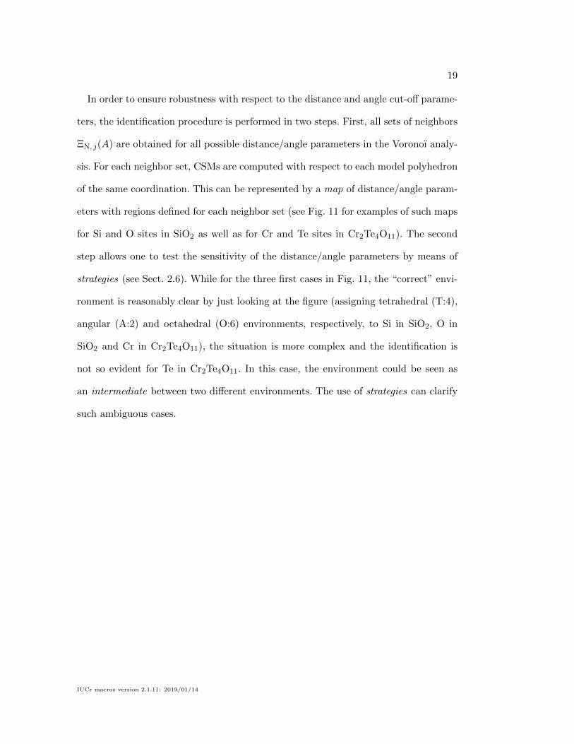
In order to ensure robustness with respect to the distance and angle cut-off parame-
ters, the identification procedure is performed in two steps. First, all sets of neighbors
ΞN, j(A) are obtained for all possible distance/angle parameters in the Voronoı analy-
sis. For each neighbor set, CSMs are computed with respect to each model polyhedron
of the same coordination. This can be represented by a map of distance/angle param-
eters with regions defined for each neighbor set (see Fig. 11 for examples of such maps
for Si and O sites in SiO2 as well as for Cr and Te sites in Cr2Te4O11). The second
step allows one to test the sensitivity of the distance/angle parameters by means of
strategies (see Sect. 2.6). While for the three first cases in Fig. 11, the “correct” envi-
ronment is reasonably clear by just looking at the figure (assigning tetrahedral (T:4),
angular (A:2) and octahedral (O:6) environments, respectively, to Si in SiO2, O in
SiO2 and Cr in Cr2Te4O11), the situation is more complex and the identification is
not so evident for Te in Cr2Te4O11. In this case, the environment could be seen as
an intermediate between two different environments. The use of strategies can clarify
such ambiguous cases.
IUCr macros version 2.1.11: 2019/01/14

20
Fig. 11. Examples of distance/angle parameters maps for Si and O in α-SiO2 (MaterialsProject id : mp-7000) and Cr and Te in Cr2Te4O11 (Materials Project id : mp-540537). Each neighbor set corresponds to a region in which any distance/angleparameters combination result in the same set. The color level of each region givesan indication of the CSM value of the model polyhedron to which the correspondingneighbor set resembles the most (i.e. for which the CSM is the lowest). For the largerregions, this model polyhedron is indicated by its symbol. The square and trianglesymbols correspond to fixed distance and angle parameters respectively of 1.3/0.6and 1.6/0.4, showing a clear ambiguity for the Te site in Cr2Te4O11 (see Sect. 2.6on how to clarify such cases).
The neighbors in each set, the CSMs for each model polyhedron in each set, and
other data related to each neighbor set are stored in a so-called StructureEnviron-
IUCr macros version 2.1.11: 2019/01/14

21
ments (see also Sect. 3) or SE (hereafter also symbolized by ΦA for atom A) object.
As exemplified in Fig. 11, this SE is not very useful as such as it contains a lot of
information that is difficult to interpret directly. In the second step presented below,
strategies are used to analyze the SE and extract usable and valuable information
from the SE.
2.6. Strategies
For the final step of the identification procedure, strategies are used to reliably
analyze the SE object and extract a useful and usable result. Reliability refers to
the robustness of our algorithm in which the sensitivity of the identification to the
distance/angle parameters is tested and challenged. Hence, the local environments
can be interpreted as one unique environment or as an intermediate between two (or
more) coordination environments, each of which being attributed a fraction or per-
centage. Different strategies can be used depending on the goals, needs and constraints
required by the user. This flexibility provided by the strategies is one of the strengths
of our identification procedure. For visualisation purposes, a strategy resulting in the
identification of a single coordination environment for each site has to be used while
reviewing the most commonly observed environments can be done with a strategy
allowing for multiple environments for the same site. One can also favour specific or
larger/smaller environments depending on the project. In the following, two strategies
are developed further.
2.6.1. Fixed distance/angle cut-offs strategy The simplest way to identify the environ-
ment is to use fixed distance and angle cut-off parameters. In this SimplestChemenv-
Strategy, the set of neighbors is thus unique and the environment is identified as the one
for which the CSM is the lowest. The advantage of such a simple procedure is that it
IUCr macros version 2.1.11: 2019/01/14

22
makes it possible to describe a local environment by its unique corresponding model
environment, which is easier to use for visualisation purposes. However, some (dis-
torted or very distorted) local environments can be considered to be an intermediate
between two or more model coordination polyhedra. In such cases, this strategy will
simply “choose” one environment, depending on the distance and angle parameters.
As a simple illustration, Fig. 12 shows the sudden switch from the square-pyramidal
environment to the octahedral environment when the distance cut-off is increased.
Similarly, for fixed distance and angle cut-offs, when an octahedron is smoothly dis-
torted by moving away one of the atoms, the resulting environment from this simplest
strategy changes abruptly from octahedral to square-pyramidal as shown in Fig. 13
(thin lines correspond to the SimplestChemenvStrategy). It is thus very sensitive to
small changes in the positions of the atoms. Nevertheless, with decent distance and
angle parameters (e.g. κ = 1.4 and γ = 0.3), the identified environment is reasonably
correct in about 85% of the cases.
IUCr macros version 2.1.11: 2019/01/14

23
1.0 1.2 1.4 1.6 1.8 2.0Distance cut-off
0.0
0.2
0.4
0.6
0.8
1.0Co
ordi
natio
n en
viro
nmen
ts fr
actio
ns3D view
Side view
=0
=0.45
=1Octahedral Squarepyramidal
Fig. 12. Coordination environments for a distorted octahedron in which the bottomatom is at distance 1.45 times larger than the other 5 neighbors. When the distancecut-off is lower than 1.45, the bottom atom is not considered as a neighbor and theenvironment is identified as a square pyramid. When the distance cut-off is largerthan 1.45, the bottom atom is taken into account and the environment is identifiedas an octahedron.
Another illustration of this strategy is shown in Fig. 14 in which a triangular prism is
smoothly distorted towards an octahedron by rotating the upper and lower triangular
planes in opposite directions (thin lines correspond to the SimplestChemenvStrategy).
In this case, the number of neighbors remains the same while the actual identified
environment switches abruptly from triangular prismatic to octahedral when the CSM
of latter becomes smaller than that of the former. Once again, the sensitivity with
respect to small changes in the positions of the atoms is critical in this strategy.
IUCr macros version 2.1.11: 2019/01/14

24
0.0 0.2 0.4 0.6 0.8 1.0
Deformation parameter α
0.0
0.2
0.4
0.6
0.8
1.0
α
OctahedralSquarepyramidalOctahedralSquarepyramidal
Side view
α=0
α=1
Coo
rdin
atio
nen
viro
nmen
tsfra
ctio
ns
Fig. 13. Smooth distortion from octahedral to square-pyramidal environment by mov-ing away the bottom atom. The deformation parameter α = 0 corresponds to theperfect octahedron while for α = 1, the bottom atom has been moved to a dis-tance that is twice that of the distance to the other neighbors. The thin lines givesthe fractions of octahedral and square-pyramidal environments obtained with theSimplestChemenvStrategy (with a distance cut-off of 1.4) while the thick lines corre-spond to the fractions obtained with the MultiWeightsChemenvStrategy. Octahedraland square-pyramidal are respectively shown as solid and dashed lines.
IUCr macros version 2.1.11: 2019/01/14

25
0.0 0.2 0.4 0.6 0.8 1.0
Deformation parameter α
0.0
0.2
0.4
0.6
0.8
1.0
OctahedralTriangularprismOctahedralTriangularprism
Side view
α0
α0α0
α1α1
α1
α1
α1α1
Coo
rdin
atio
nen
viro
nmen
tsfra
ctio
ns
Fig. 14. Smooth distortion from triangular prismatic to octahedral environment bytwisting the triangular prism around the principal axis. The deformation parameterα = 0 corresponds to the perfect trigonal prism while for α = 1, the upper (red →orange) and lower (green→ cyan) triangles have been rotated respectively clockwiseand counterclockwise by 30, corresponding to an octahedron. The thin lines givesthe fractions of triangular prismatic and octahedral environments obtained with theSimplestChemenvStrategy while the thick lines correspond to the fractions obtainedwith the MultiWeightsChemenvStrategy. Octahedral and triangular prismatic arerespectively shown as solid and dashed lines.
2.6.2. Strategy based on multiple weights A second strategy is developed hereafter, in
which special care has been taken to remove the artificial abrupt transitions observed
with the SimplestChemenvStrategy. The idea is to smooth these transitions using a
combination of smooth step functions. A given local environment can thus be identified
either as one unique coordination environment if distortions are small, or as a mix of
two or more environments for larger distortions. In practice, the local environment is
described as a list of environments, each being assigned a fraction or percentage.
IUCr macros version 2.1.11: 2019/01/14

26
The percentage or fraction fE(A) of a given model coordination environment E
depends on the results (CSMs, Voronoı parameters, . . . ) for each possible set of neigh-
bors contained in ΦA.
fE(A) = f [ΦA](E) (2)
The procedure used to get the fraction of a model polyhedron E for a given local
environment is then obtained as the product of two terms. Suppose E occurs in a given
neighbor set Ξ. The first term results from the relative weight of the neighbor set (as
compared to the other neighbor sets) displaying model environment E . The second
term comes from the relative weight of the model polyhedron E within that specific
neighbor set.
f [ΦA](E) = fouter[ΦA]× f inner[ΞNA ](E) (3)
In the following, the first term is referred to as the outer weight (i.e. the weight that
depends on other so-called outer neighbor sets) and the second term is referred to as
the inner weight (i.e. the weight inside a specific neighbor set).
Inner weight For a given neighbor set ΞNA of atom A in a given coordination N , the
relative weight (and hence fraction) of each model polyhedron is not straightforward.
Let ΘN be the set of K model environments with coordination N :
ΘN = EN1 , . . . , ENi , . . . , ENK (4)
For example, the set Θ6 of six-coordinated model polyhedra (as reported in Refs. (Hartshorn
et al., 2007) and (Lima-de Faria et al., 1990) and implemented in the ChemEnv pack-
age) is composed of the octahedron (symbolized O:6), the trigonal prism (symbolized
T:6) and the pentagonal pyramid (symbolized PP:6).
IUCr macros version 2.1.11: 2019/01/14

27
For each model polyhedron ENi , the CSM SENi[ΞNA ] with respect to the local envi-
ronment ΞNA is used to assign a weight to each model polyhedron thanks to the use
of an adequately shaped function. Model environments with a lower CSM (i.e. more
similar to the local environment) are assigned a larger weight. In particular, if one
of the model environments has a CSM of 0.0 (i.e. the local environment is perfect),
its weight should be infinite so that it is the only model environment identified. The
function should also allow for the assignment of a zero weight to a model polyhedron
for which the CSM is larger than a given maximum value Smax. One example of such
a function is the “modified” inverse function defined in Eqn. 5 and shown in Fig. 15.
wSmax(S) =
1/Smax × (S−Smax)2
S if S ≤ Smax,
0.0 if S > Smax.(5)
in which the numerator (S − Smax)2 ensures the continuity at S = Smax while the
prefactor 1/Smax arises from the normalization of the [0, Smax] to [0, 1].
0 2 4 6 8 10 12
Continuous symmetry measure
0
2
4
6
8
10
12
Wei
ght
fun
ctio
n
O:6
T :6PP :6
Continuous symmetry measures :
SO:6 = 0.78ST :6 = 4.3SPP :6 = 11.5
Weights :
wO:6 = 8.354wT :6 = 0.398wPP :6 = 0.0
Weights sum : 8.752
Fractions :fO:6 = 8.354/8.752 = 0.955fT :6 = 0.398/8.752 = 0.045fPP :6 = 0.0/8.752 = 0.0
Example
Fig. 15. Weight function for the inner weight of model polyhedra. In this example,Smax is set to 8.0, so that the weight of any model polyhedron with a CSM largerthan 8.0 is zero.
IUCr macros version 2.1.11: 2019/01/14

28
Fractions of each model environment E i are then obtained from these weights:
f inner[ΞNA ](E i) =wSmax(SEi)∑j=Kj=1 wSmax(SEj )
(6)
A small example is also given in Fig. 15 in which CSMs for a fictitious six-coordinated
case are provided.
When the coordination is clearly defined (i.e. when only one neighbor set is identified
using the procedure outlined in 2.5), the fractions of each model polyhedron are solely
determined by this inner weight. On the other hand, when different neighbor sets are
identified, an additional complexity arises from the fact that smaller environments
usually tend to be more easily recognized as similar (i.e. having smaller CSMs). The
extreme case is the single neighbor which is always assigned a CSM of zero. For cases
in which more than one neighbor set is present, the outer weight is used to determine
the relative predominance of each of the neighbor sets (and hence their corresponding
model polyhedron).
Outer weight The outer weight or neighbor set weight refers to the weight of a given
neighbor set with respect to the other neighbor sets. This outer weight is defined as a
product of several “partial weights” (the definition being general enough to allow for
flexibility in the choice of the weights) :
wouter[ΨA](ΞA) =i=nw∏
i=1
wi[ΨA](ΞA) (7)
in which nw is the number of partial weights used.
Some of the partial neighbor set weights compare the CSMs of this neighbor set with
the ones for the other neighbor sets. The simplest approach is to take the smallest
CSM for each of the neighbor sets. In practice, to ensure continuity, an effective CSM
is defined. The effective CSM of a given neighbor set ΞNA , denoted Seff(ΞNA ), is obtained
IUCr macros version 2.1.11: 2019/01/14
29
from a weighted average using the “modified” inverse function defined in Eqn. 5.
Seff(ΞNA ) =
∑E∈ΘN
wSmax(SE)× SE∑E∈ΘN
wSmax(SE)(8)
in which SE is a short form for SE(ΞNA ), i.e. the CSM of the neighbor set with respect
to the perfect environment E .
Partial weights In the following, the partial weights used in the “default” multi-
weights strategy (used in a previous publication (Waroquiers et al., 2017)) are described.
The strategy with these default parameters is easily obtained with the following class
method (see examples in the tutorials provided in the supplementary material):
MultiWeightsChemenvStrategy.stats article weights parameters()
Other weights have also been implemented in the ChemEnv package in pymatgen.
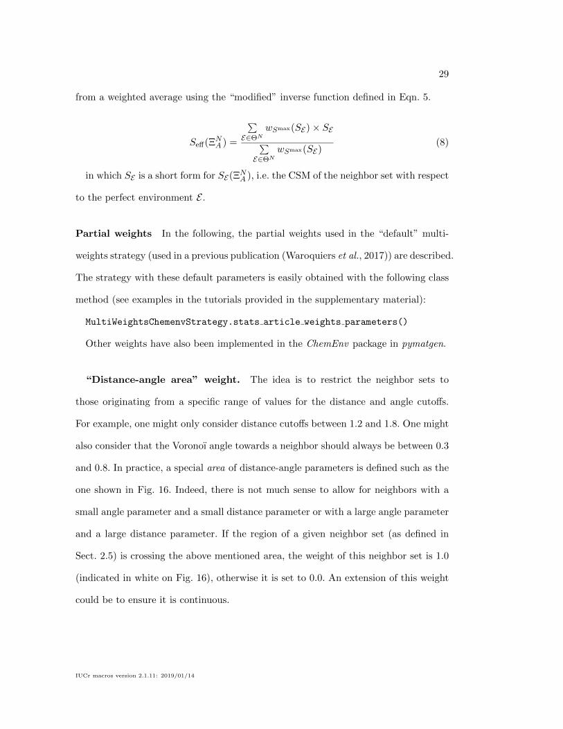
“Distance-angle area” weight. The idea is to restrict the neighbor sets to
those originating from a specific range of values for the distance and angle cutoffs.
For example, one might only consider distance cutoffs between 1.2 and 1.8. One might
also consider that the Voronoı angle towards a neighbor should always be between 0.3
and 0.8. In practice, a special area of distance-angle parameters is defined such as the
one shown in Fig. 16. Indeed, there is not much sense to allow for neighbors with a
small angle parameter and a small distance parameter or with a large angle parameter
and a large distance parameter. If the region of a given neighbor set (as defined in
Sect. 2.5) is crossing the above mentioned area, the weight of this neighbor set is 1.0
(indicated in white on Fig. 16), otherwise it is set to 0.0. An extension of this weight
could be to ensure it is continuous.
IUCr macros version 2.1.11: 2019/01/14

30
1.0 1.2 1.4 1.6 1.8 2.0 2.2 2.4
Distance parameter : κ
0.0
0.2
0.4
0.6
0.8
1.0
An
gle
par
amet
er:γ
0
2
4
6
8
10
CS
M
Fig. 16. Schematic of the distance-angle area weight. The shaded area is used todetermine which neighbor sets are considered. If the region of a given neighbor setis crossing the shaded area, the set is assigned a “distance-angle area” weight of1.0. In the opposite case, the set is assigned a weight of 0.0 (white regions).
“Self CSM” weight. This weight makes use of the effective CSM Seff of each
neighbor set defined in Eqn. 8. Each neighbor set is assigned a weight depending on
the value of this effective Seff . The idea is to disfavour neighbor sets that are globally
more distorted than others. One example function used to estimate this weight is
defined in Eqn. 9 and shown in Fig. 17.
wSmax,λ(Seff) =
(Seff − 1.0)2 × e−λSeff if Seff ≤ 1.0,
0.0 if Seff > 1.0.(9)
where Seff is the normalized effective CSM defined as SeffSmax
.
IUCr macros version 2.1.11: 2019/01/14

31
0 2 4 6 8 10 12Effective Continuous symmetry measure Seff
0.0
0.2
0.4
0.6
0.8
1.0W
eigh
tfu
nct
ion
Smax = 8.0λ = 1.0Smax = 5.0λ = 1.0Smax = 8.0λ = 0.2
Fig. 17. Weight function for the Self-CSM outer weight of neighbor sets as defined inEqn. 9. The default parameters for this weight are shown as blue while the greenand purple curves illustrate other parameters. Arrows indicate thresholds abovewhich values (i.e. Smax) of the effective CSM Seff each of the weight functions areset to zero.
“Delta CSM” weight. The goal of this neighbor set weight is to reduce the
importance of a given neighbor set ΞN1 if another neighbor set ΞN2 of larger coordi-
nation number N2 > N1 is present and not too distorted with respect to the first one.
In practice, this weight depends on the difference ∆Seff between the effective CSMs
(as defined in Eqn. 8) of the neighbor sets ΞN2 and ΞN1 :
∆Seff(ΞN1 ,ΞN2) = Seff(ΞN2)− Seff(ΞN1) (10)
The Delta CSM weight is defined as :
wdeltaχ;∆min,∆max [ΦA](ΞA) = minΞi∈ΦA;
N(Ξi)>N(ΞA)
χ∆min,∆max (∆Seff(ΞA,Ξi)) (11)
IUCr macros version 2.1.11: 2019/01/14

32
in which χ is a sigmoid-like function (e.g. a smooth step or smoother step function),
N(Ξ) is the coordination of neighbor set Ξ and ∆min, ∆max are the edges used in the
χ function.
An example of a χ function is the smoother step function shown in Fig. 18 and
defined as :
χsmootherstepa,b (x) =
0.0 if x ≤ a,6x5 − 15x4 + 10x3 if a < x < b,
1.0 if x ≥ b.(12)
in which x = (x − a)/(b − a) is the scaled value of x mapping the [a, b] interval to
the [0, 1] interval.
0 2 4 6 8
∆Seff (Ξ1,Ξ2) = Seff (Ξ2)− Seff (Ξ1)
0.0
0.2
0.4
0.6
0.8
1.0
Del
taC
SM
Wei
ght
ofΞ
1
∆min = 1.0∆max = 4.0
∆min = 4.0∆max = 6.0
∆min = 3.0∆max = 8.0
Fig. 18. Smoother step function used in the Delta CSM weight. The ”Delta CSM”weight assigned to the Ξ1 neighbor set is equal to 0.0 if the difference ∆Seff(Ξ1,Ξ2)between the effective CSM Seff(Ξ2) of the Ξ2 neighbor set and its own effective CSMSeff(Ξ1) is lower than ∆min. If the difference ∆Seff(Ξ1,Ξ2) is larger than ∆min, theΞ1 set is assigned a weight of 1.0. The smoother step function is used between thesetwo extremes. The ∆min and ∆max values can be changed if needed and examplesof smoother step functions for different values are shown.
IUCr macros version 2.1.11: 2019/01/14

33
Choice of partial weights The default list of outer weights consists of the three
above-mentioned partial weights. As an example and in particular to illustrate the
need to use both the Self CSM weight and the Delta CSM weight, Fig. 19 shows the
fractions of environments obtained for different choices of weights in the case of the
smooth distortion from octahedral to square-pyramidal environment (see Fig. 13).
0.0
2.0
4.0
6.0
8.0
CS
M
OctahedralSquare pyramidal
0.0
0.2
0.4
0.6
0.8
1.0
Env
ironm
ents
fract
ions
Strategy including onlythe SelfCSM weight
0.0
0.2
0.4
0.6
0.8
1.0
Sel
fCS
Mw
eigh
t
0.0
0.2
0.4
0.6
0.8
1.0
Env
ironm
ents
fract
ions
Strategy including onlythe DeltaCSM weight
0.0 0.2 0.4 0.6 0.8 1.0
0.0
0.2
0.4
0.6
0.8
1.0
Del
taC
SM
wei
ght
0.0 0.2 0.4 0.6 0.8 1.0
0.0
0.2
0.4
0.6
0.8
1.0
Env
ironm
ents
fract
ions
Strategy includingboth weights
0.0 0.2 0.4 0.6 0.8 1.0
Deformation parameter α
0.0
0.2
0.4
0.6
0.8
1.0
Fig. 19. Choice of partial weights: comparison and combination of Self CSM andDelta CSM weights in the case of the smooth distortion from octahedral tosquare-pyramidal environment. Curves in blue (green) correspond to the octahe-dral (square-pyramidal) environment. See text for details.
The upper left panel shows the CSM of the octahedral (increasing with the dis-
tortion) and square-pyramidal (always equal to 0.0). The middle left and lower left
IUCr macros version 2.1.11: 2019/01/14

34
panels show the Self CSM and Delta CSM weights for both environments. The Self
CSM weight for the square-pyramidal environment is always 1.0 as its CSM is always
0.0. Conversely, the Delta CSM weight for the octahedral environment is always 1.0
as there is no larger neighbor set to be compared to. As shown in the upper right
panel, when the sole Self CSM weight is included, the fractions obtained are 50%
octahedral and 50% square-pyramidal when no or little distortion is applied (while
one would expect to have 100% octahedral and 0% square-pyramidal). Indeed, for both
environments, the value of the CSM is 0.0 and hence the Self CSM weight is 1.0. At
variance, the middle right panel illustrates the fractions obtained when the sole Delta
CSM weight is included. In that case, for large distortions, the fractions obtained are
also 50% for each environment. Indeed, when the distortion is large, the Delta CSM
weight for the square-pyramidal environment reaches 1.0 as the larger environment is
too distorted to disfavour the square-pyramidal environment. The lower right panel
illustrates the case when both the Self CSM and Delta CSM weights are included.
3. Description of the package
The ChemEnv module is written in Python and can be found in the pymatgen package
(Ong et al., 2013) as part of the analysis submodule. The organisation of the package
is shown diagrammatically in Fig. 20. The description of each of the objects referenced
as circled numbers in this figure is given hereafter :
1 LocalGeometryFinder
Main class used to identify the local environments in a structure.
2 AllCoordinationGeometries
Class containing the list of all the available model coordination geometries (as
CoordinationGeometry objects, see 3).
IUCr macros version 2.1.11: 2019/01/14

35
3 CoordinationGeometry
Generic class for the description of all the model coordination geometries. An
instance of this class is created for each model environment (from the json files
stored in the coordination geometry files directory). It contains information
about its perfect coordinates as well as its edges and faces, name(s), symbol(s),
technical details for the identification procedure, . . .
4 StructureEnvironments
Class containing the information (CSMs, neighbors, . . . ) on all possible neighbor
sets for all sites in the structure as introduced in Sect. 2.5. This object is meant
to be post-processed with a strategy in order to get relevant and usable data
about the local environments of the structure.
5 LightStructureEnvironments
Class containing the processed data from the StructureEnvironments class using
one strategy. This object lists the environment(s) and their corresponding frac-
tions (in case of a strategy allowing for mixtures of environments) for each site
of the structure.
6 DetailedVoronoiContainer
Class containing the information on the Voronoı analysis (see Sect. 2.2) per-
formed at the beginning of the identification procedure in order to define the
different possible neighbor sets.
7 SimplestChemenvStrategy
Class used to apply the fixed distance/angle cutoff strategy introduced in Sect. 2.6.1.
8 MultiWeightsChemenvStrategy
IUCr macros version 2.1.11: 2019/01/14

36
Class used to apply the strategy based on multiple weights as introduced in
Sect. 2.6.2.
IUCr macros version 2.1.11: 2019/01/14

37
pymatgen
analysis
chemenv
coordination environments
coordination geometry files
A#2.json
AC#12.json
...
strategy files
...
tests
...
coordination geometry finder.py
LocalGeometryFinder 1
. . .
coordination geometries.py
AllCoordinationGeometries 2
CoordinationGeometry 3
. . .
structure environments.py
StructureEnvironments 4
LightStructureEnvironments 5
. . .
voronoi.py
DetailedVoronoiContainer 6
chemenv strategies.py
SimplestChemenvStrategy 7
MultiWeightsChemenvStrategy 8
. . .
utils
tests
......
Fig. 20. Organisation of the ChemEnv package. Directories are indicated in black andsurrounded by a rectangle. Files are indicated in typewriter (blue for python files,purple for other files). The most important python objects are indicated in italic(green). See text for more information.
IUCr macros version 2.1.11: 2019/01/14
38
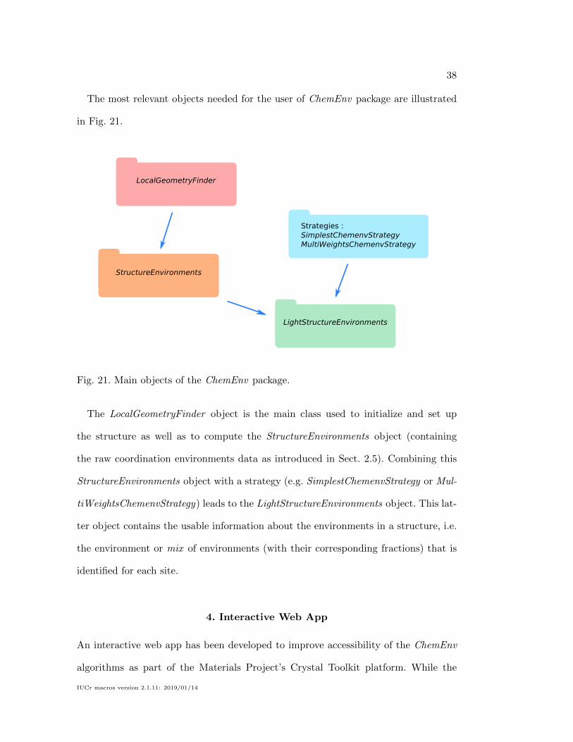
The most relevant objects needed for the user of ChemEnv package are illustrated
in Fig. 21.
Fig. 21. Main objects of the ChemEnv package.
The LocalGeometryFinder object is the main class used to initialize and set up
the structure as well as to compute the StructureEnvironments object (containing
the raw coordination environments data as introduced in Sect. 2.5). Combining this
StructureEnvironments object with a strategy (e.g. SimplestChemenvStrategy or Mul-
tiWeightsChemenvStrategy) leads to the LightStructureEnvironments object. This lat-
ter object contains the usable information about the environments in a structure, i.e.
the environment or mix of environments (with their corresponding fractions) that is
identified for each site.
4. Interactive Web App
An interactive web app has been developed to improve accessibility of the ChemEnv
algorithms as part of the Materials Project’s Crystal Toolkit platform. While the
IUCr macros version 2.1.11: 2019/01/14

39
Python interface is intuitive and well-documented, not all scientists are Python users,
and the web app enables use of ChemEnv by any user without installing custom soft-
ware. The web app supports uploading of any file format supported by the pymatgen
code, including Crystallographic Information Format (CIF). Alternatively, structures
can be loaded directly from the Materials Project database containing more than
100,000 inorganic materials.
The web app is designed to offer one-to-one equivalent functionality to ChemEnv by
directly calling the corresponding pymatgen interface, specifically using the LightStruc-
tureEnvironments and SimplestChemenvStrategy, and allowing the user full interactive
control over the distance and angle cut-offs. Each symmetrically distinct chemical envi-
ronment is shown in 3D using a custom atomic visualizer, along with Wyckoff label,
IUPAC symbol, CSM, and human-readable environment label. Oxidation states will
be used in the analysis if atoms are appropriately annotated in the uploaded file or,
if these are not supplied, oxidation states can be guessed on-the-fly using pymatgen’s
bond valence analysis algorithms. It will be hosted by the Materials Project, and is
available at http://crystaltoolkit.org .
5. Conclusion
We have developed a tool that can analye coordination or local environments of large
numbers of crystal structures in a fast and robust manner. The analysis of the neigh-
boring atoms relies on a modified Voronoı approach on a grid of distance and angle
cutoffs. On this grid of different distance and angle cutoffs, the coordination envi-
ronments are determined with the help of a similtarity metric to the shape of ideal
polyhedra. Two different strategies are implemented to arrive at the final assignment
of the coordination environments. One of these strategies is especially robust against
small distortions of the crystal structures making the algorithm particularly useful for
IUCr macros version 2.1.11: 2019/01/14

40
automatic, unsupervised, local environment assignment. This new tool can be used as
part of the open-source Python library (pymatgen) and within an interactive web app
available on http://crystaltoolkit.org through the Materials Project.
6. Supplementary Information
A tutorial for the ChemEnv package both in pdf- and jupyter-notebook format is avail-
able in the Supplementary Information. The list of all environments as well as some
details about the implementation are also available in the Supplementary Information.
J. G. acknowledges funding from the European Union’s Horizon 2020 research and
innovation program under the Marie Sk lodowska-Curie grant agreement No 837910.
Integration with the Materials Project infrastructure was supported by by the U.S.
Department of Energy, Office of Science, Office of Basic Energy Sciences, Materials
Sciences and Engineering Division under Contract No. DE-AC02-05CH11231 (Mate-
rials Project program KC23MP).
References
Allmann, R. & Hinek, R. (2007). Acta Cryst. A, 63(5), 412–417.URL: https://doi.org/10.1107/S0108767307038081
Bergerhoff, G. & Brown, I. D. (1987). Crystallographic databases, vol. 360, pp. 77–95.
Brunner, G. O. & Schwarzenbach, D. (1971). Z. Kristallogr. - Cryst. Mater. 133(1-6), 127.URL: https://www.degruyter.com/view/j/zkri.1971.133.issue-1-6/zkri.1971.133.16.127/zkri.1971.133.16.127.xml
Lima-de Faria, J., Hellner, E., Liebau, F., Makovicky, E. & Parthe, E. (1990). Acta Cryst. A,46(1), 1–11.URL: http://dx.doi.org/10.1107/S0108767389008834
Francois Pomerleau, F. C. & Siegwart, R. (2015). A Review of Point Cloud Registration Algo-rithms for Mobile Robotics.
Groom, C. R. & Allen, F. H. (2014). Angew. Chem. Int. Ed. 53(3), 662–671.URL: http://dx.doi.org/10.1002/anie.201306438
Hartshorn, R. M., Hey-Hawkins, E., Kalio, R. & Leigh, G. J. (2007). Pure Appl. Chem. 79(10),1779–1799.URL: http://iupac.org/publications/pac/79/10/1779/
Hoffmann, R. (1987). Angew. Chem. Int. Ed. 26(9), 846.
Hoffmann, R. (1988). Solids and surfaces: a chemist’s view of bonding in extended structures.
Hoppe, R. (1979). Z. Kristallogr. - Cryst. Mater. 150(1-4), 23.URL: https://www.degruyter.com/view/j/zkri.1979.150.issue-1-4/zkri.1979.150.14.23/zkri.1979.150.14.23.xml
IUCr macros version 2.1.11: 2019/01/14

41
Jain, A., Hautier, G., Ong, S. P. & Persson, K. (2016). J. Mater. Res. 31(8), 977.
Jain, A., Ong, S. P., Hautier, G., Chen, W., Richards, W. D., Dacek, S., Cholia, S., Gunter,D., Skinner, D., Ceder, G. & Persson, K. a. (2013). APL Mater. 1(1), 011002.URL: http://link.aip.org/link/AMPADS/v1/i1/p011002/s1&Agg=doi
Kabsch, W. (1976). Acta Cryst. A32(5), 922–923.
Kabsch, W. (1978). Acta Cryst. A34(5), 827–828.
Lueken, H. (2013). Magnetochemie: Eine Einfuhrung in Theorie und Anwendung. TeubnerStudienbucher Chemie. Vieweg+Teubner Verlag.URL: https://books.google.be/books?id=JMT1BQAAQBAJ
Maiseli, B., Gu, Y. & Gao, H. (2017). J. Visual Commun. Image Represent. 46(SupplementC), 95 – 106.URL: http://www.sciencedirect.com/science/article/pii/S1047320317300743
Muller, U. (2007). Inorganic Structural Chemistry. Wiley.URL: https://books.google.de/books?id=s3KlfXCY11sC
O’Keefe, M. (1979). Acta Cryst. A, 35(1978), 772–775.
Ong, S. P., Richards, W. D., Jain, A., Hautier, G., Kocher, M., Cholia, S., Gunter, D., Chevrier,V. L., Persson, K. A. & Ceder, G. (2013). Comput. Mater. Sci. 68(0), 314–319.URL: http://www.sciencedirect.com/science/article/pii/S0927025612006295
Pauling, L. (1929). J. Am. Chem. Soc. 51(4), 1010.URL: https://doi.org/10.1021/ja01379a006
Peng, H., Ndione, P. F., Ginley, D. S., Zakutayev, A. & Lany, S. (2015). Phys. Rev. X, 5,021016.URL: https://link.aps.org/doi/10.1103/PhysRevX.5.021016
Pfeiffer, P. (1915). Z. Anorg. Allg. Chem. 92(1), 376–380.URL: https://doi.org/10.1002/zaac.19150920126
Pfeiffer, P. (1916). Z. Anorg. Allg. Chem. 97(1), 161–174.URL: https://doi.org/10.1002/zaac.19160970112
Pinsky, M. & Avnir, D. (1998). Inorg. Chem. 37(21), 5575–5582.URL: http://pubs.acs.org/doi/abs/10.1021/ic9804925
Stoiber, D. & Niewa, R. (2019). Z. Kristallogr. - Cryst. Mater. 0(0).URL: https://www.degruyter.com/view/j/zkri.ahead-of-print/zkri-2018-2115/zkri-2018-2115.xml
Villars, P. & Cenzual, K. (2018). Pearson’s Crystal Data: Crystal Structure Database forInorganic Compounds (on DVD), Release 2018/19. ASM International, Materials Park,Ohio, USA.
Waroquiers, D., Gonze, X., Rignanese, G.-M., Welker-Nieuwoudt, C., Rosowski, F., Gobel,M., Schenk, S., Degelmann, P., Andre, R., Glaum, R. & Hautier, G. (2017). Chem. Mat.29(19), 8346.URL: https://doi.org/10.1021/acs.chemmater.7b02766
Zimmermann, N. E. R., Horton, M. K., Jain, A. & Haranczyk, M. (2017). Front. Mater. 4,34.URL: https://www.frontiersin.org/article/10.3389/fmats.2017.00034
Synopsis
We present a new tool called ChemEnv, which can identify coordination environments in afast and robust manner.
IUCr macros version 2.1.11: 2019/01/14

download fileview on ChemRxivpaper.pdf (4.27 MiB)

Acta Crystallographica Section A
Foundations ofCrystallographyISSN 0108-7673
c© 0000 International Union of CrystallographyPrinted in Singapore – all rights reserved
Supporting Information for ”ChemEnv : A fast androbust coordination environment identification tool”David Waroquiers,a Janine George,a Matthew Horton,b,c Stephan Schenk,d
Kristin A. Persson,b,c Gian-Marco Rignanese,a Xavier Gonzea,e and Geof-froy Hautier a*aInstitute of Condensed Matter and Nanosciences, Universite catholique de Louvain, Chemin des Etoiles
8, 1348 Louvain-la-Neuve, Belgium, bEnergy Technologies Area, Lawrence Berkeley National Laboratory,
Berkeley, CA 94720, USA, cDepartment of Materials Science and Engineering, University of California,
Berkeley, CA 94720, USA, dBASF SE, Digitalization of R&D, Carl-Bosch-Str. 38, 67056 Ludwigshafen,
Germany, and eSkolkovo Institute of Science and Technology, Skolkovo Innovation Center, Nobel St. 3,
Moscow, 143026, Russia. Correspondence e-mail: [email protected]
This supplementary information describes the different coordination environmentsidentified by ChemEnv and provides technical details about the identification pro-cedure.
1. Model coordination environments and separationplanes
The following lists the model coordination environments foreach coordination number. For each model coordination envi-ronment, the symbol used in ChemEnv, a descriptive name, thecoordinates of the points, the IUCr and IUPAC symbols as wellas technical details about the algorithm used for the identifica-tion are provided.
Coordination 1• S:1→ Single neighbor
IUCr symbol : [1l]IUPAC symbol : NonePoints :
A 0.0000 0.0000 1.0000
Explicit permutations algorithm
Coordination 2• L:2→ Linear
IUCr symbol : [2l]IUPAC symbol : L-2Points :
A 0.0000 0.0000 1.0000B 0.0000 0.0000 −1.0000
Explicit permutations algorithm
• A:2→ AngularIUCr symbol : [2n]IUPAC symbol : A-2Points :
A 1.0000 0.0000 0.0000B −0.5000 0.8660 0.0000
Explicit permutations algorithm
Coordination 3• TL:3→ Trigonal plane
IUCr symbol : [3l]IUPAC symbol : TP-3Points :
A 0.0000 1.0000 0.0000B 0.8660 −0.5000 0.0000C −0.8660 −0.5000 0.0000
Explicit permutations algorithm
• TY:3→ Triangular non-coplanarIUCr symbol : [3n]IUPAC symbol : TPY-3Points :
A 0.5774 −0.5774 −0.5774B −0.5774 0.5774 −0.5774C −0.5774 −0.5774 0.5774
Explicit permutations algorithm
• TS:3→ T-shapedIUCr symbol : NoneIUPAC symbol : TS-3Points :
A −1.0000 0.0000 0.0000B 1.0000 0.0000 0.0000C 0.0000 0.0000 1.0000
Explicit permutations algorithm
Acta Cryst. (0000). A00, 000000 LIST OF AUTHORS · (SHORTENED) TITLE 1

Coordination 4• T:4→ Tetrahedron
IUCr symbol : [4t]IUPAC symbol : T-4Points :
A 0.5774 −0.5774 −0.5774B −0.5774 0.5774 −0.5774C −0.5774 −0.5774 0.5774D 0.5774 0.5774 0.5774
Explicit permutations algorithm
• S:4→ Square planeIUCr symbol : [4l]IUPAC symbol : SP-4Points :
A 1.0000 0.0000 0.0000B −1.0000 0.0000 0.0000C 0.0000 1.0000 0.0000D 0.0000 −1.0000 0.0000
Explicit permutations algorithm
• SY:4→ Square non-coplanarIUCr symbol : [4n]IUPAC symbol : SPY-4Points :
A 0.9258 0.0000 0.3780B −0.9258 0.0000 0.3780C 0.0000 0.9258 0.3780D 0.0000 −0.9258 0.3780
Explicit permutations algorithm
• SS:4→ See-sawIUCr symbol : NoneIUPAC symbol : SS-4Points :
A 1.0000 0.0000 0.0000B 0.0000 0.8660 0.5000C 0.0000 0.0000 −1.0000D −1.0000 0.0000 0.0000
Explicit permutations algorithm
Coordination 5• PP:5→ Pentagonal plane
IUCr symbol : [5l]IUPAC symbol : PP-5Points :
A 1.0000 0.0000 0.0000B 0.3090 0.9511 0.0000C −0.8090 0.5878 0.0000D −0.8090 −0.5878 0.0000E 0.3090 −0.9511 0.0000
Explicit permutations algorithm
• S:5→ Square pyramidIUCr symbol : [5y]IUPAC symbol : SPY-5Points :
A 1.0000 0.0000 0.0000B −1.0000 0.0000 0.0000C 0.0000 1.0000 0.0000D 0.0000 −1.0000 0.0000E 0.0000 0.0000 1.0000
Explicit permutations algorithm
• T:5→ Trigonal bipyramidIUCr symbol : [5by]IUPAC symbol : TBPY-5Points :
A 0.0000 1.0000 0.0000B 0.8660 −0.5000 0.0000C −0.8660 −0.5000 0.0000D 0.0000 0.0000 1.0000E 0.0000 0.0000 −1.0000
Explicit permutations algorithm
Coordination 6• O:6→ Octahedron
IUCr symbol : [6o]IUPAC symbol : OC-6Points :
A 0.0000 0.0000 1.0000B 0.0000 0.0000 −1.0000C 1.0000 0.0000 0.0000D −1.0000 0.0000 0.0000E 0.0000 1.0000 0.0000F 0.0000 −1.0000 0.0000
Separation plane algorithms :
Ô E / ACBD / F
Ô ∅ / ACE / FBD
• T:6→ Trigonal prismIUCr symbol : [6p]IUPAC symbol : TPR-6Points :
A −0.6547 −0.3780 0.6547B 0.6547 −0.3780 0.6547C 0.0000 0.7559 0.6547D −0.6547 −0.3780 −0.6547E 0.6547 −0.3780 −0.6547F 0.0000 0.7559 −0.6547
Separation plane algorithms :
Ô ∅ / ABED / CF
Ô ∅ / ABC / DEF
2 LIST OF AUTHORS · (SHORTENED) TITLE Acta Cryst. (0000). A00, 000000
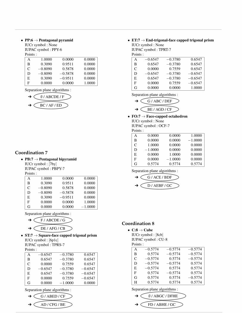
• PP:6→ Pentagonal pyramidIUCr symbol : NoneIUPAC symbol : PPY-6Points :
A 1.0000 0.0000 0.0000B 0.3090 0.9511 0.0000C −0.8090 0.5878 0.0000D −0.8090 −0.5878 0.0000E 0.3090 −0.9511 0.0000F 0.0000 0.0000 1.0000
Separation plane algorithms :
Ô ∅ / ABCDE / F
Ô BC / AF / ED
Coordination 7• PB:7→ Pentagonal bipyramid
IUCr symbol : [7by]IUPAC symbol : PBPY-7Points :
A 1.0000 0.0000 0.0000B 0.3090 0.9511 0.0000C −0.8090 0.5878 0.0000D −0.8090 −0.5878 0.0000E 0.3090 −0.9511 0.0000F 0.0000 0.0000 1.0000G 0.0000 0.0000 −1.0000
Separation plane algorithms :
Ô F / ABCDE / G
Ô DE / AFG / CB
• ST:7→ Square-face capped trigonal prismIUCr symbol : [6p1c]IUPAC symbol : TPRS-7Points :
A −0.6547 −0.3780 0.6547B 0.6547 −0.3780 0.6547C 0.0000 0.7559 0.6547D −0.6547 −0.3780 −0.6547E 0.6547 −0.3780 −0.6547F 0.0000 0.7559 −0.6547G 0.0000 −1.0000 0.0000
Separation plane algorithms :
Ô G / ABED / CF
Ô AD / CFG / BE
• ET:7→ End-trigonal-face capped trigonal prismIUCr symbol : NoneIUPAC symbol : TPRT-7Points :
A −0.6547 −0.3780 0.6547B 0.6547 −0.3780 0.6547C 0.0000 0.7559 0.6547D −0.6547 −0.3780 −0.6547E 0.6547 −0.3780 −0.6547F 0.0000 0.7559 −0.6547G 0.0000 0.0000 1.0000
Separation plane algorithms :
Ô G / ABC / DEF
Ô BE / AGD / CF
• FO:7→ Face-capped octahedronIUCr symbol : NoneIUPAC symbol : OCF-7Points :
A 0.0000 0.0000 1.0000B 0.0000 0.0000 −1.0000C 1.0000 0.0000 0.0000D −1.0000 0.0000 0.0000E 0.0000 1.0000 0.0000F 0.0000 −1.0000 0.0000G 0.5774 0.5774 0.5774
Separation plane algorithms :
Ô G / ACE / BDF
Ô D / AEBF / GC
Coordination 8• C:8→ Cube
IUCr symbol : [8cb]IUPAC symbol : CU-8Points :
A −0.5774 −0.5774 −0.5774B 0.5774 −0.5774 −0.5774C −0.5774 0.5774 −0.5774D −0.5774 −0.5774 0.5774E −0.5774 0.5774 0.5774F 0.5774 −0.5774 0.5774G 0.5774 0.5774 −0.5774H 0.5774 0.5774 0.5774
Separation plane algorithms :
Ô ∅ / ABGC / DFHE
Ô FD / ABHE / GC
Acta Cryst. (0000). A00, 000000 LIST OF AUTHORS · (SHORTENED) TITLE 3

• SA:8→ Square antiprismIUCr symbol : [8acb]IUPAC symbol : SAPR-8Points :
A 0.0000 0.8595 0.5111B 0.0000 −0.8595 0.5111C 0.8595 0.0000 0.5111D −0.8595 0.0000 0.5111E 0.6078 0.6078 −0.5111F 0.6078 −0.6078 −0.5111G −0.6078 0.6078 −0.5111H −0.6078 −0.6078 −0.5111
Separation plane algorithms :
Ô ∅ / ACBD / EFHG
Ô E / ACFG / DBH
• SBT:8→ Square-face bicapped trigonal prismIUCr symbol : NoneIUPAC symbol : TPRS-8Points :
A −0.6547 −0.3780 0.6547B 0.6547 −0.3780 0.6547C 0.0000 0.7559 0.6547D −0.6547 −0.3780 −0.6547E 0.6547 −0.3780 −0.6547F 0.0000 0.7559 −0.6547G 0.8660 0.5000 0.0000H −0.8660 0.5000 0.0000
Separation plane algorithms :
Ô ∅ / ABED / CGFH
Ô H / ACFD / BGE
• TBT:8→ Triangular-face bicapped trigonal prismIUCr symbol : [6p2c]IUPAC symbol : TPRT-8Points :
A −0.6547 −0.3780 0.6547B 0.6547 −0.3780 0.6547C 0.0000 0.7559 0.6547D −0.6547 −0.3780 −0.6547E 0.6547 −0.3780 −0.6547F 0.0000 0.7559 −0.6547G 0.0000 0.0000 1.0000H 0.0000 0.0000 −1.0000
Separation plane algorithm :
Ô AD / CFHG / BE
• DD:8→ Dodecahedron with triangular facesIUCr symbol : [8do]IUPAC symbol : DD-8Points :
A −0.5000 0.0000 −0.7839B 0.5000 0.0000 −0.7839C 0.0000 −0.6446 −0.2056D 0.0000 0.6446 −0.2056E −0.6446 0.0000 0.2056F 0.6446 0.0000 0.2056G 0.0000 −0.5000 0.7839H 0.0000 0.5000 0.7839
Separation plane algorithm :
Ô CG / ABFE / DH
• DDPN:8→ Dodecahedron with triangular faces - p2345 planenormalizedIUCr symbol : NoneIUPAC symbol : NonePoints :
A −0.5000 0.0000 −0.7839B 0.5000 0.0000 −0.7839C 0.0000 −0.9068 −0.2056D 0.0000 0.9068 −0.2056E −0.9068 0.0000 0.2056F 0.9068 0.0000 0.2056G 0.0000 −0.5000 0.7839H 0.0000 0.5000 0.7839
Separation plane algorithm :
Ô CG / ABFE / DH
• HB:8→ Hexagonal bipyramidIUCr symbol : [8by]IUPAC symbol : HBPY-8Points :
A 1.0000 0.0000 0.0000B 0.5000 0.8660 0.0000C −0.5000 0.8660 0.0000D −1.0000 0.0000 0.0000E −0.5000 −0.8660 0.0000F 0.5000 −0.8660 0.0000G 0.0000 0.0000 1.0000H 0.0000 0.0000 −1.0000
Separation plane algorithms :
Ô G / ABCDEF / H
Ô FE / AHDG / BC
4 LIST OF AUTHORS · (SHORTENED) TITLE Acta Cryst. (0000). A00, 000000
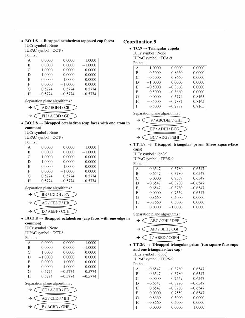
• BO 1:8→ Bicapped octahedron (opposed cap faces)IUCr symbol : NoneIUPAC symbol : OCT-8Points :
A 0.0000 0.0000 1.0000B 0.0000 0.0000 −1.0000C 1.0000 0.0000 0.0000D −1.0000 0.0000 0.0000E 0.0000 1.0000 0.0000F 0.0000 −1.0000 0.0000G 0.5774 0.5774 0.5774H −0.5774 −0.5774 −0.5774
Separation plane algorithms :
Ô AD / EGFH / CB
Ô FH / ACBD / GE
• BO 2:8 → Bicapped octahedron (cap faces with one atom incommon)IUCr symbol : NoneIUPAC symbol : OCT-8Points :
A 0.0000 0.0000 1.0000B 0.0000 0.0000 −1.0000C 1.0000 0.0000 0.0000D −1.0000 0.0000 0.0000E 0.0000 1.0000 0.0000F 0.0000 −1.0000 0.0000G 0.5774 0.5774 0.5774H 0.5774 −0.5774 −0.5774
Separation plane algorithms :
Ô BE / CGDH / FA
Ô AG / CEDF / HB
Ô D / AEBF / CGH
• BO 3:8 → Bicapped octahedron (cap faces with one edge incommon)IUCr symbol : NoneIUPAC symbol : OCT-8Points :
A 0.0000 0.0000 1.0000B 0.0000 0.0000 −1.0000C 1.0000 0.0000 0.0000D −1.0000 0.0000 0.0000E 0.0000 1.0000 0.0000F 0.0000 −1.0000 0.0000G 0.5774 −0.5774 0.5774H 0.5774 −0.5774 −0.5774
Separation plane algorithms :
Ô CE / AGHB / FD
Ô AG / CEDF / BH
Ô E / ACBD / GHF
Coordination 9• TC:9→ Triangular cupola
IUCr symbol : NoneIUPAC symbol : TCA-9Points :
A 1.0000 0.0000 0.0000B 0.5000 0.8660 0.0000C −0.5000 0.8660 0.0000D −1.0000 0.0000 0.0000E −0.5000 −0.8660 0.0000F 0.5000 −0.8660 0.0000G 0.0000 0.5774 0.8165H −0.5000 −0.2887 0.8165I 0.5000 −0.2887 0.8165
Separation plane algorithms :
Ô ∅ / ABCDEF / GHI
Ô EF / ADHI / BCG
Ô BC / ADG / FEHI
• TT 1:9 → Tricapped triangular prism (three square-facecaps)IUCr symbol : [6p3c]IUPAC symbol : TPRS-9Points :
A −0.6547 −0.3780 0.6547B 0.6547 −0.3780 0.6547C 0.0000 0.7559 0.6547D −0.6547 −0.3780 −0.6547E 0.6547 −0.3780 −0.6547F 0.0000 0.7559 −0.6547G 0.8660 0.5000 0.0000H −0.8660 0.5000 0.0000I 0.0000 −1.0000 0.0000
Separation plane algorithms :
Ô ABC / GHI / DEF
Ô AID / BEH / CGF
Ô I / ABED / CGFH
• TT 2:9 → Tricapped triangular prism (two square-face capsand one triangular-face cap)IUCr symbol : [6p3c]IUPAC symbol : TPRS-9Points :
A −0.6547 −0.3780 0.6547B 0.6547 −0.3780 0.6547C 0.0000 0.7559 0.6547D −0.6547 −0.3780 −0.6547E 0.6547 −0.3780 −0.6547F 0.0000 0.7559 −0.6547G 0.8660 0.5000 0.0000H −0.8660 0.5000 0.0000I 0.0000 0.0000 1.0000
Acta Cryst. (0000). A00, 000000 LIST OF AUTHORS · (SHORTENED) TITLE 5

Separation plane algorithms :
Ô AD / HIBE / CGF
Ô GEB / CFI / HDA
• TT 3:9 → Tricapped triangular prism (one square-face capand two triangular-face caps)IUCr symbol : [6p3c]IUPAC symbol : TPRS-9Points :
A −0.6547 −0.3780 0.6547B 0.6547 −0.3780 0.6547C 0.0000 0.7559 0.6547D −0.6547 −0.3780 −0.6547E 0.6547 −0.3780 −0.6547F 0.0000 0.7559 −0.6547G 0.0000 −1.0000 0.0000H 0.0000 0.0000 −1.0000I 0.0000 0.0000 1.0000
Separation plane algorithms :
Ô AD / IGHFC / BE
Ô CF / BEHI / AGD
• HD:9→ Heptagonal dipyramidIUCr symbol : NoneIUPAC symbol : HBPY-9Points :
A 1.0000 0.0000 0.0000B 0.6235 0.7818 0.0000C −0.2225 0.9749 0.0000D −0.9010 0.4339 0.0000E −0.9010 −0.4339 0.0000F −0.2225 −0.9749 0.0000G 0.6235 −0.7818 0.0000H 0.0000 0.0000 1.0000I 0.0000 0.0000 −1.0000
Separation plane algorithm :
Ô H / ABCDEFG / I
• TI:9→ Tridiminished icosahedronIUCr symbol : NoneIUPAC symbol : NonePoints :
A 0.0000 0.5257 0.8507B 0.0000 0.5257 −0.8507C 0.0000 −0.5257 −0.8507D 0.5257 0.8507 0.0000E 0.5257 −0.8507 0.0000F −0.5257 −0.8507 0.0000G 0.8507 0.0000 0.5257H −0.8507 0.0000 0.5257I −0.8507 0.0000 −0.5257
Separation plane algorithms :
Ô GE / AFCD / HIB
Ô B / CDI / EGAHF
• SMA:9→ Square-face monocapped antiprismIUCr symbol : NoneIUPAC symbol : SAPRS-9Points :
A 0.0000 0.8595 0.5111B 0.0000 −0.8595 0.5111C 0.8595 0.0000 0.5111D −0.8595 0.0000 0.5111E 0.6078 0.6078 −0.5111F 0.6078 −0.6078 −0.5111G −0.6078 0.6078 −0.5111H −0.6078 −0.6078 −0.5111I 0.0000 0.0000 −1.0000
Separation plane algorithms :
Ô AGE / CDI / BHF
Ô I / EFHG / CBDA
Ô CBF / EHI / ADG
• SS:9→ Square-face capped square prismIUCr symbol : NoneIUPAC symbol : CUS-9Points :
A −0.5774 −0.5774 −0.5774B 0.5774 −0.5774 −0.5774C −0.5774 0.5774 −0.5774D −0.5774 −0.5774 0.5774E −0.5774 0.5774 0.5774F 0.5774 −0.5774 0.5774G 0.5774 0.5774 −0.5774H 0.5774 0.5774 0.5774I 0.0000 0.0000 1.0000
Separation plane algorithms :
Ô BF / ADIHG / CE
Ô I / DEHF / ACGB
Ô BG / ACHF / DEI
• TO 1:9 → Tricapped octahedron (all 3 cap faces share oneatom)IUCr symbol : NoneIUPAC symbol : TOCT-9Points :
A 0.0000 0.0000 1.0000B 0.0000 0.0000 −1.0000C 1.0000 0.0000 0.0000D −1.0000 0.0000 0.0000E 0.0000 1.0000 0.0000F 0.0000 −1.0000 0.0000G 0.5774 0.5774 0.5774H 0.5774 −0.5774 0.5774I 0.5774 −0.5774 −0.5774
6 LIST OF AUTHORS · (SHORTENED) TITLE Acta Cryst. (0000). A00, 000000

Separation plane algorithms :
Ô IBF / CDH / GEA
Ô BE / CGDI / AFH
Ô DF / AHIB / GCE
• TO 2:9→ Tricapped octahedron (cap faces are aligned)IUCr symbol : NoneIUPAC symbol : TOCT-9Points :
A 0.0000 0.0000 1.0000B 0.0000 0.0000 −1.0000C 1.0000 0.0000 0.0000D −1.0000 0.0000 0.0000E 0.0000 1.0000 0.0000F 0.0000 −1.0000 0.0000G 0.5774 0.5774 0.5774H 0.5774 −0.5774 0.5774I −0.5774 −0.5774 −0.5774
Separation plane algorithms :
Ô CB / EGHFI / AD
Ô EB / CGDI / HAF
• TO 3:9 → Tricapped octahedron (all 3 cap faces aresharingone edge of a face)IUCr symbol : NoneIUPAC symbol : TOCT-9Points :
A 0.0000 0.0000 1.0000B 0.0000 0.0000 −1.0000C 1.0000 0.0000 0.0000D −1.0000 0.0000 0.0000E 0.0000 1.0000 0.0000F 0.0000 −1.0000 0.0000G 0.5774 0.5774 0.5774H −0.5774 0.5774 −0.5774I 0.5774 −0.5774 −0.5774
Separation plane algorithms :
Ô CGA / FIE / BHD
Ô AF / DGCI / HEB
Coordination 10• PP:10→ Pentagonal prism
IUCr symbol : NoneIUPAC symbol : PPR-10Points :
A 1.0000 0.0000 −0.5878B 0.3090 0.9511 −0.5878C −0.8090 0.5878 −0.5878D −0.8090 −0.5878 −0.5878E 0.3090 −0.9511 −0.5878F 1.0000 0.0000 0.5878G 0.3090 0.9511 0.5878H −0.8090 0.5878 0.5878I −0.8090 −0.5878 0.5878J 0.3090 −0.9511 0.5878
Separation plane algorithms :
Ô ∅ / ABCDE / FGHIJ
Ô BG / ACHF / EDIJ
• PA:10→ Pentagonal antiprismIUCr symbol : NoneIUPAC symbol : PAPR-10Points :
A 1.0000 0.0000 −0.4253B 0.3090 0.9511 −0.4253C −0.8090 0.5878 −0.4253D −0.8090 −0.5878 −0.4253E 0.3090 −0.9511 −0.4253F 0.8090 0.5878 0.4253G −0.3090 0.9511 0.4253H −1.0000 0.0000 0.4253I −0.3090 −0.9511 0.4253J 0.8090 −0.5878 0.4253
Separation plane algorithms :
Ô ∅ / ABCDE / FGHIJ
Ô DIH / CEJG / BAF
• SBSA:10→ Square-face bicapped square antiprismIUCr symbol : NoneIUPAC symbol : SAPRS-10Points :
A 0.0000 0.8595 0.5111B 0.0000 −0.8595 0.5111C 0.8595 0.0000 0.5111D −0.8595 0.0000 0.5111E 0.6078 0.6078 −0.5111F 0.6078 −0.6078 −0.5111G −0.6078 0.6078 −0.5111H −0.6078 −0.6078 −0.5111I 0.0000 0.0000 −1.0000J 0.0000 0.0000 1.0000
Separation plane algorithms :
Acta Cryst. (0000). A00, 000000 LIST OF AUTHORS · (SHORTENED) TITLE 7
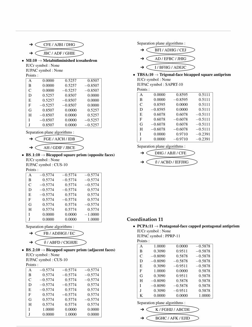
Ô CFE / AJBI / DHG
Ô JBC / ADF / GHIE
• MI:10→Metabidiminished icosahedronIUCr symbol : NoneIUPAC symbol : NonePoints :
A 0.0000 0.5257 0.8507B 0.0000 0.5257 −0.8507C 0.0000 −0.5257 −0.8507D 0.5257 0.8507 0.0000E 0.5257 −0.8507 0.0000F −0.5257 −0.8507 0.0000G 0.8507 0.0000 0.5257H −0.8507 0.0000 0.5257I −0.8507 0.0000 −0.5257J 0.8507 0.0000 −0.5257
Separation plane algorithms :
Ô FGE / AJCH / IDB
Ô AH / GDIF / JBCE
• BS 1:10→ Bicapped square prism (opposite faces)IUCr symbol : NoneIUPAC symbol : CUS-10Points :
A −0.5774 −0.5774 −0.5774B 0.5774 −0.5774 −0.5774C −0.5774 0.5774 −0.5774D −0.5774 −0.5774 0.5774E −0.5774 0.5774 0.5774F 0.5774 −0.5774 0.5774G 0.5774 0.5774 −0.5774H 0.5774 0.5774 0.5774I 0.0000 0.0000 −1.0000J 0.0000 0.0000 1.0000
Separation plane algorithms :
Ô FB / ADJHGI / EC
Ô ∅ / ABFD / CIGHJE
• BS 2:10→ Bicapped square prism (adjacent faces)IUCr symbol : NoneIUPAC symbol : CUS-10Points :
A −0.5774 −0.5774 −0.5774B 0.5774 −0.5774 −0.5774C −0.5774 0.5774 −0.5774D −0.5774 −0.5774 0.5774E −0.5774 0.5774 0.5774F 0.5774 −0.5774 0.5774G 0.5774 0.5774 −0.5774H 0.5774 0.5774 0.5774I 1.0000 0.0000 0.0000J 0.0000 1.0000 0.0000
Separation plane algorithms :
Ô BFI / ADHG / CEJ
Ô AD / EFBC / JHIG
Ô I / BFHG / ADEJC
• TBSA:10→ Trigonal-face bicapped square antiprismIUCr symbol : NoneIUPAC symbol : SAPRT-10Points :
A 0.0000 0.8595 0.5111B 0.0000 −0.8595 0.5111C 0.8595 0.0000 0.5111D −0.8595 0.0000 0.5111E 0.6078 0.6078 −0.5111F 0.6078 −0.6078 −0.5111G −0.6078 0.6078 −0.5111H −0.6078 −0.6078 −0.5111I 0.0000 0.9710 −0.2391J 0.0000 −0.9710 −0.2391
Separation plane algorithms :
Ô DHG / ABJI / CFE
Ô ∅ / ACBD / IEFJHG
Coordination 11• PCPA:11→ Pentagonal-face capped pentagonal antiprism
IUCr symbol : NoneIUPAC symbol : PPRP-11Points :
A 1.0000 0.0000 −0.5878B 0.3090 0.9511 −0.5878C −0.8090 0.5878 −0.5878D −0.8090 −0.5878 −0.5878E 0.3090 −0.9511 −0.5878F 1.0000 0.0000 0.5878G 0.3090 0.9511 0.5878H −0.8090 0.5878 0.5878I −0.8090 −0.5878 0.5878J 0.3090 −0.9511 0.5878K 0.0000 0.0000 1.0000
Separation plane algorithms :
Ô K / FGHIJ / ABCDE
Ô BGHC / AFK / EJID
8 LIST OF AUTHORS · (SHORTENED) TITLE Acta Cryst. (0000). A00, 000000

• H:11→ HendecahedronIUCr symbol : NoneIUPAC symbol : NonePoints :
A 0.0000 0.0000 2.0000B 2.0000 1.0000 1.0000C 0.0000 −1.0000 1.0000D −2.0000 1.0000 1.0000E 0.0000 2.0000 0.0000F 1.0000 −1.0000 0.0000G −1.0000 −1.0000 0.0000H 2.0000 1.0000 −1.0000I 0.0000 −1.0000 −1.0000J −2.0000 1.0000 −1.0000K 0.0000 0.0000 −2.0000
Separation plane algorithm :
Ô DGJ / EACIK / BFH
• DI:11→ Diminished icosahedronIUCr symbol : NoneIUPAC symbol : NonePoints :
A 0.0000 −1.0000 −1.6180B 0.0000 1.0000 −1.6180C 0.0000 −1.0000 1.6180D 0.0000 1.0000 1.6180E −1.0000 −1.6180 0.0000F 1.0000 −1.6180 0.0000G −1.0000 1.6180 0.0000H 1.0000 1.6180 0.0000I −1.6180 0.0000 −1.0000J −1.6180 0.0000 1.0000K 1.6180 0.0000 −1.0000
Separation plane algorithms :
Ô I / GJEAB / DCFKH
Ô FHK / ACDB / EJGI
Coordination 12• I:12→ Icosahedron
IUCr symbol : [12i]IUPAC symbol : IC-12Points :
A 0.0000 −1.0000 −1.6180B 0.0000 1.0000 −1.6180C 0.0000 −1.0000 1.6180D 0.0000 1.0000 1.6180E −1.0000 −1.6180 0.0000F 1.0000 −1.6180 0.0000G −1.0000 1.6180 0.0000H 1.0000 1.6180 0.0000I −1.6180 0.0000 −1.0000J −1.6180 0.0000 1.0000K 1.6180 0.0000 −1.0000L 1.6180 0.0000 1.0000
Separation plane algorithm :
Ô EIGJ / ABDC / FKHL
• PBP:12→ Pentagonal-face bicapped pentagonal prismIUCr symbol : NoneIUPAC symbol : PPRP-12Points :
A 1.0000 0.0000 −0.5878B 0.3090 0.9511 −0.5878C −0.8090 0.5878 −0.5878D −0.8090 −0.5878 −0.5878E 0.3090 −0.9511 −0.5878F 1.0000 0.0000 0.5878G 0.3090 0.9511 0.5878H −0.8090 0.5878 0.5878I −0.8090 −0.5878 0.5878J 0.3090 −0.9511 0.5878K 0.0000 0.0000 −1.0000L 0.0000 0.0000 1.0000
Separation plane algorithm :
Ô EJID / AFLK / BGHC
• TT:12→ Truncated tetrahedronIUCr symbol : [12tt]IUPAC symbol : NonePoints :
A −0.5774 0.5774 −1.7321B 0.5774 −0.5774 −1.7321C −0.5774 −1.7321 0.5774D 0.5774 −1.7321 −0.5774E 1.7321 0.5774 0.5774F 1.7321 −0.5774 −0.5774G −1.7321 −0.5774 0.5774H −1.7321 0.5774 −0.5774I 0.5774 1.7321 0.5774J −0.5774 1.7321 −0.5774K 0.5774 0.5774 1.7321L −0.5774 −0.5774 1.7321
Acta Cryst. (0000). A00, 000000 LIST OF AUTHORS · (SHORTENED) TITLE 9
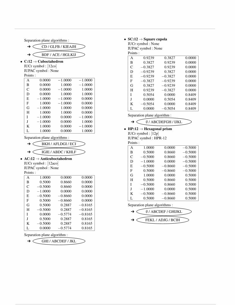
Separation plane algorithms :
Ô CD / GLFB / KIEAJH
Ô BDF / ACE / HGLKIJ
• C:12→ CuboctahedronIUCr symbol : [12co]IUPAC symbol : NonePoints :
A 0.0000 −1.0000 −1.0000B 0.0000 1.0000 −1.0000C 0.0000 −1.0000 1.0000D 0.0000 1.0000 1.0000E −1.0000 −1.0000 0.0000F 1.0000 −1.0000 0.0000G −1.0000 1.0000 0.0000H 1.0000 1.0000 0.0000I −1.0000 0.0000 −1.0000J −1.0000 0.0000 1.0000K 1.0000 0.0000 −1.0000L 1.0000 0.0000 1.0000
Separation plane algorithms :
Ô BKH / AFLDGI / ECJ
Ô IGJE / ABDC / KHLF
• AC:12→ AnticuboctahedronIUCr symbol : [12aco]IUPAC symbol : NonePoints :
A 1.0000 0.0000 0.0000B 0.5000 0.8660 0.0000C −0.5000 0.8660 0.0000D −1.0000 0.0000 0.0000E −0.5000 −0.8660 0.0000F 0.5000 −0.8660 0.0000G 0.5000 0.2887 −0.8165H −0.5000 0.2887 −0.8165I 0.0000 −0.5774 −0.8165J 0.5000 0.2887 0.8165K −0.5000 0.2887 0.8165L 0.0000 −0.5774 0.8165
Separation plane algorithm :
Ô GHI / ABCDEF / JKL
• SC:12→ Square cupolaIUCr symbol : NoneIUPAC symbol : NonePoints :
A 0.9239 0.3827 0.0000B 0.3827 0.9239 0.0000C −0.3827 0.9239 0.0000D −0.9239 0.3827 0.0000E −0.9239 −0.3827 0.0000F −0.3827 −0.9239 0.0000G 0.3827 −0.9239 0.0000H 0.9239 −0.3827 0.0000I 0.5054 0.0000 0.8409J 0.0000 0.5054 0.8409K −0.5054 0.0000 0.8409L 0.0000 −0.5054 0.8409
Separation plane algorithm :
Ô ∅ / ABCDEFGH / IJKL
• HP:12→ Hexagonal prismIUCr symbol : [12p]IUPAC symbol : HPR-12Points :
A 1.0000 0.0000 −0.5000B 0.5000 0.8660 −0.5000C −0.5000 0.8660 −0.5000D −1.0000 0.0000 −0.5000E −0.5000 −0.8660 −0.5000F 0.5000 −0.8660 −0.5000G 1.0000 0.0000 0.5000H 0.5000 0.8660 0.5000I −0.5000 0.8660 0.5000J −1.0000 0.0000 0.5000K −0.5000 −0.8660 0.5000L 0.5000 −0.8660 0.5000
Separation plane algorithms :
Ô ∅ / ABCDEF / GHIJKL
Ô FEKL / ADJG / BCIH
10 LIST OF AUTHORS · (SHORTENED) TITLE Acta Cryst. (0000). A00, 000000

• HA:12→ Hexagonal antiprismIUCr symbol : NoneIUPAC symbol : HAPR-12Points :
A 1.0000 0.0000 −0.4278B 0.5000 0.8660 −0.4278C −0.5000 0.8660 −0.4278D −1.0000 0.0000 −0.4278E −0.5000 −0.8660 −0.4278F 0.5000 −0.8660 −0.4278G 0.8660 0.5000 0.4278H 0.0000 1.0000 0.4278I −0.8660 0.5000 0.4278J −0.8660 −0.5000 0.4278K 0.0000 −1.0000 0.4278L 0.8660 −0.5000 0.4278
Separation plane algorithm :
Ô ∅ / ABCDEF / GHIJKL
Coordination 13• SH:13→ Square-face capped hexagonal prism
IUCr symbol : NoneIUPAC symbol : NonePoints :
A 1.0000 0.0000 −0.5000B 0.5000 0.8660 −0.5000C −0.5000 0.8660 −0.5000D −1.0000 0.0000 −0.5000E −0.5000 −0.8660 −0.5000F 0.5000 −0.8660 −0.5000G 1.0000 0.0000 0.5000H 0.5000 0.8660 0.5000I −0.5000 0.8660 0.5000J −1.0000 0.0000 0.5000K −0.5000 −0.8660 0.5000L 0.5000 −0.8660 0.5000M 0.9682 −0.5590 0.0000
Separation plane algorithm :
Ô ∅ / ABCDEF / GHIJKLM
Acta Cryst. (0000). A00, 000000 LIST OF AUTHORS · (SHORTENED) TITLE 11

download fileview on ChemRxivsupplementary_information.pdf (159.36 KiB)