Chemical characteristics and causes of airborne particulate pollution

Atmos. Chem. Phys., 16, 10671–10687, 2016www.atmos-chem-phys.net/16/10671/2016/doi:10.5194/acp-16-10671-2016© Author(s) 2016. CC Attribution 3.0 License.

Chemical characteristics and causes of airborne particulatepollution in warm seasons in Wuhan, central ChinaXiaopu Lyu1, Nan Chen2, Hai Guo1, Lewei Zeng1, Weihao Zhang3, Fan Shen2, Jihong Quan2, and Nan Wang4

1Department of Civil and Environmental Engineering, The Hong Kong Polytechnic University, Hong Kong, Hong Kong2Hubei Provincial Environment Monitoring Center, Wuhan, China3Department of Environmental Sciences, School of Resource and Environmental Sciences, Wuhan University, Wuhan, China4Guangdong Provincial Key Laboratory of Regional Numerical Weather Prediction, Institute of Tropical and MarineMeteorology, Guangzhou, China

Correspondence to: Hai Guo ([email protected])

Received: 8 January 2016 – Published in Atmos. Chem. Phys. Discuss.: 4 March 2016Revised: 16 August 2016 – Accepted: 16 August 2016 – Published: 29 August 2016

Abstract. Continuous measurements of airborne particlesand their chemical compositions were conducted in May,June, October, and November 2014 at an urban site inWuhan, central China. The results indicate that particle con-centrations remained at a relatively high level in Wuhan,with averages of 135.1± 4.4 (mean± 95 % confidence in-terval) and 118.9± 3.7 µg m−3 for PM10 and 81.2± 2.6 and85.3± 2.6 µg m−3 for PM2.5 in summer and autumn, respec-tively. Moreover, PM2.5 levels frequently exceeded the Na-tional Standard Level II (i.e., daily average of 75 µg m−3),and six PM2.5 episodes (i.e., daily PM2.5 averages above75 µg m−3 for 3 or more consecutive days) were capturedduring the sampling campaign. Potassium was the mostabundant element in PM2.5, with an average concentra-tion of 2060.7± 82.3 ng m−3; this finding indicates inten-sive biomass burning in and around Wuhan during the studyperiod, because almost no correlation was found betweenpotassium and mineral elements (iron and calcium). Thesource apportionment results confirm that biomass burningwas the main cause of episodes 1, 3, and 4, with contri-butions to PM2.5 of 46.6 %± 3.0 %, 50.8 %± 1.2 %, and44.8 %± 2.6%, respectively, whereas fugitive dust was theleading factor in episode 2. Episodes 5 and 6 resulted mainlyfrom increases in vehicular emissions and secondary inor-ganic aerosols, and the mass and proportion of NO−3 bothpeaked during episode 6. The high levels of NOx and NH3and the low temperature during episode 6 were responsiblefor the increase of NO−3 . Moreover, the formation of sec-ondary organic carbon was found to be dominated by aromat-

ics and isoprene in autumn, and the contribution of aromaticsto secondary organic carbon increased during the episodes.

1 Introduction

Airborne particulate pollution, also called “haze”, has sweptacross China in recent years, particularly over its northern,central, and eastern parts (Cheng et al., 2014; Kang et al.,2013; Wang et al., 2013). Due to its detrimental effects onhuman health (Anderson et al., 2012; Goldberg et al., 2001),the atmosphere (Yang et al., 2012; White and Roberts, 1977),acid precipitation (Zhang et al., 2007; Kerminen et al., 2001),and climate change (Ramanathan et al., 2001; Nemesure etal., 1995), particulate pollution has become a major concernof scientific communities and local governments. China’s na-tional ambient air quality standards issued in 2012 regulatethe annual upper limit of PM10 (i.e., particulate matter withan aerodynamic diameter of less than 10 µm) and PM2.5 (i.e.,particulate matter with an aerodynamic diameter of less than2.5 µm) as 70 and 35 µg m−3 and 24 h averages as 150 and75 µg m−3, respectively (GB 3095-2012, 2016).

Numerous studies have been conducted in China to un-derstand the spatiotemporal variations in particle concen-trations, the chemical composition, and the causes of hazeevents (Cheng et al., 2014; Cao et al., 2012; Zheng et al.,2005; Yao et al., 2002). In general, particulate pollution ismore severe in winter due to additional emissions (e.g., coalburning) and unfavorable dispersion conditions (Lyu et al.,

Published by Copernicus Publications on behalf of the European Geosciences Union.

10672 X. Lyu et al.: Chemical characteristics and causes of airborne particulate pollution

2015a; Zheng et al., 2005). Northern China often suffersheavier, longer, and more frequent haze pollution than south-ern China (Cao et al., 2012). Chemical analysis indicatesthat secondary inorganic aerosol (SIA; i.e., sulfate [SO2−

4 ],nitrate [NO−3 ], and ammonium [NH+4 ]) and secondary or-ganic aerosol (SOA) dominate the total mass of airborne par-ticles (Zhang et al., 2014, 2012). However, the compositiondiffers among the size-segregated particles. In general, sec-ondary species and mineral or sea salt components are proneto be apportioned in fine and coarse particles (Zhang et al.,2013; Theodosi et al., 2011). Indeed, the general characteris-tics of particles (e.g., toxicity, radiative forcing, acidity) areall tightly associated with their chemical compositions andphysical sizes, which therefore have been extensively studiedin the field of aerosols. To better understand and control air-borne particulate pollution, the causes and formation mech-anisms have often been investigated (Wang et al., 2014a, b;Kang et al., 2013; Oanh and Leelasakultum, 2011). Apartfrom the unfavorable meteorological conditions, emissionenhancement was often the major culprit. There is little doubtthat industrial and vehicular emissions contributed greatly tothe particle mass via direct emission and secondary forma-tion of particles from gaseous precursors, such as sulfur diox-ide (SO2), nitrogen oxides (NOx), and volatile organic com-pounds (VOCs; Guo et al., 2011a). In addition, some othersources in specific regions or during specific time periodshave also built up the particle concentrations to a remark-able degree, e.g., coal combustion in north China (Cao etal., 2005; Zheng et al., 2005) and biomass burning in South-east Asia (Deng et al., 2008; Koe et al., 2001). Furthermore,some studies have explored the possible formation mecha-nisms of the main particle components (SIA and SOA) anddistinguished the contributions of different formation path-ways. For example, Y. X. Wang et al. (2014) demonstratedthat heterogeneous oxidation of SO2 on aerosol surfaces wasan important supplementary pathway to particle-bound SO2−

4in addition to gas phase oxidation and reactions in clouds.In contrast, it was reported that homogeneous and hetero-geneous reactions dominated the formation of NO−3 duringthe day and night, respectively (Pathak et al., 2011; Lin etal., 2010; Seinfeld and Pandis, 1998). Furthermore, biogenicVOCs and aromatics were shown to be the main precursorsof SOA (Kanakidou et al., 2005; Forstner et al., 1997).

Despite numerous studies, the full components of airborneparticles have seldom been reported due to the cost of sam-pling and chemical analysis, resulting in a gap in our under-standing of the chemical characteristics of particles. In addi-tion, although the causes of particle episodes have been dis-cussed in many case studies (Y. X. Wang et al., 2014; Denget al., 2008), the contributions have rarely been quantified.Furthermore, the formation mechanisms might differ in var-ious circumstances. Therefore, an overall understanding ofthe chemical characteristics of airborne particles, the causesof the particle episodes, and the formation mechanisms of the

enhanced species would be of great value. In addition, thefrequent occurrence of haze pollution has become a regularphenomenon in central China during warm seasons, but thecauses have not been identified and the contributions havenot been quantified. Wuhan is the largest megacity in cen-tral China and has suffered from severe particulate pollutionin recent years. The data indicate that the frequency of daysin which PM2.5 exceeded the national standard level II (i.e.,a daily average of 75 µg m−3) in Wuhan reached 55.1 % in2014 (Wuhan Environmental Bulletin, 2014). In the warmseasons of 2014, the hourly maximum PM2.5 (564 µg m−3)was even higher than that in winter (383 µg m−3), as shownin Fig. S1 in the Supplement. Moreover, because the air qual-ity in Wuhan is strongly influenced by the surrounding cities,the pollution level in Wuhan also reflects the status of the cityclusters in central China. However, previous studies (Lyu etal., 2015a; Cheng et al., 2014) did not allow a complete un-derstanding of the properties of airborne particles in this re-gion, particularly during the warm seasons, nor could theyguide control strategies. It is therefore urgent to understandthe chemical characteristics of airborne particles and to ex-plore the causes and formation mechanisms of the particleepisodes in Wuhan.

This study comprehensively analyzed the chemical char-acteristics of PM2.5 in Wuhan from a full suite of com-ponent measurement data: SO2−

4 , NO−3 , NH+4 , organic car-bon (OC), including primary organic carbon (POC) and sec-ondary organic carbon (SOC), elemental carbon (EC), andelements. Furthermore, based on the analysis of meteorolog-ical conditions, chemical signatures, source apportionment,and distribution of wildfires, the causes of the PM2.5 episodesare identified and their contributions quantified. Finally, thisstudy used a photochemical box model incorporating a mas-ter chemical mechanism (PBM-MCM) and theoretical cal-culation to investigate the formation processes of NO−3 andSOC. Ours is the first study to quantify the contribution ofbiomass burning to PM2.5 and examine the formation mech-anisms of both inorganic and organic components in PM2.5in central China.

2 Methods

2.1 Data collection

The whole set of air pollutants were continuously monitoredat an urban site in the largest megacity of central China,i.e., Wuhan. The measurement covered two periods: Mayand June in summer and October and November in autumnof 2014. The measured species included particle-phase pol-lutants such as PM10, PM2.5, and particle-bound compo-nents and gas-phase pollutants, including VOCs, SO2, CO,NO, NO2, O3, HNO3(g), NH3(g), and HCl(g). Hourly datawere obtained for each species. The sampling site (30.54◦ N,114.37◦ E) was located in the Hubei Environmental Moni-

Atmos. Chem. Phys., 16, 10671–10687, 2016 www.atmos-chem-phys.net/16/10671/2016/

X. Lyu et al.: Chemical characteristics and causes of airborne particulate pollution 10673

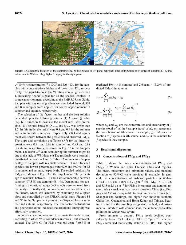
toring Center Station, as shown in Fig. 1, located in a mixedcommercial and residential area in which industries are sel-dom permitted. The instruments were housed in a room ina six-story building (∼ 18 m above ground level) adjacent toa main road at a straight-line distance of ∼ 15 m. The trafficvolume of the road was around 200 vehicles per hour. How-ever, a wall (∼ 2 m high) and several rows of trees (7 to 8 mhigh) were located between the road and the sampling site.

PM10 and PM2.5 were measured with a continuous ambi-ent particulate monitor (Thermo Fisher-1405D, USA) inte-grated with a filter dynamics measurement system to mini-mize the loss of semivolatile particulate matter. The water-soluble ions (WSIs) in PM2.5 and gases including HNO3,HCl, and NH3 were detected with an online ion chromatog-raphy monitor (Metrohm-MARGA 1S, Switzerland). How-ever, data were not available in May and June, because theinstrument was initially deployed in September. An aerosolOC/EC online analyzer (Sunset-RT-4, USA); the NIOSHthermal-optical transmission method was used to resolve thecarbonaceous aerosols (OC and EC). In addition, the ele-ments in PM2.5 were measured with a customized metalanalyzer. This instrument used a PM2.5 impactor to col-lect the airborne particulate samples, which were analyzedby the β-ray in terms of mass concentrations. The filtersloaded with particles were then sent to an X-ray fluorescenceanalysis system for quantitative analysis. K+ monitored bythe online ion chromatography correlated well (R2

= 0.88;slope= 0.80) with K monitored by the customized metal ana-lyzer. To keep consistency with other elements, K rather thanK+ was used to do the following analyses in this study. Forthe analysis of trace gases (SO2, CO, NO, NO2, and O3), weused a suite of commercial analyzers developed by ThermoEnvironmental Instruments Inc., which have been describedin detail (Lyu et al., 2016; Geng et al., 2009). Furthermore,a gas chromatography–flame ionization detector–mass spec-trometry system (TH_PKU-300) was used to resolve the realtime data of the ambient VOCs. The details of the analysistechniques, resolution, detection limits, and the protocol ofquality assurance/control were provided by Lyu et al. (2016)and H. L. Wang et al. (2014).

2.2 Theoretical calculation and model simulation

Theoretical calculation and model simulation were applied inthis study to examine the formation mechanisms of NO−3 andSOC. The particle-bound NO−3 was generally combined withNH3 or presented as HNO3 in the ammonia-deficient envi-ronment, following the processes described in Reaction (R1)through Reaction (R3) after HNO3 was formed by the ox-idation of NOx (Pathak et al., 2011; Lin et al., 2010). Theproduction of NO−3 can be calculated with Eqs. (1)–(4).

NH3(g)+HNO3(g)↔ NH4NO3(s)k1 (R1)

= exp[118.87− 24 084/T − 6.025ln(T )] (ppb2)

NH3(g)+HNO3(g)↔ NH+4 +NO−3 k2 (R2)

= (P1−P2(1− aw)+P3(1− aw)2)

× (1− aw)(1− aw)1.75k1 (ppb2)

N2O5+H2O→ 2HNO3k3 (R3)

= γ /4(8kT /πmN2O5)0.5Ap (s−1)

ln(P1)=−135.94+ 8763/T + 19.12ln(T ) (1)ln(P2)=−122.65+ 9969/T + 16.22ln(T ) (2)ln(P3)=−182.61+ 13875/T + 24.46ln(T ) (3)[NO−3

]= 0.775 (4)[NH3]+[HNO3

]−

√([NH3

]+ [HNO3]

)2− 4

([NH3][HNO3

]− k1(k2)

)2

,where Reactions (R1) and (R2) describe the homogeneousformation of NO−3 in humidity conditions lower and higherthan the deliquescence relative humidity of NH4NO3 (i.e.,62 %; Tang and Munkelwitz, 1993), respectively. Reac-tion (R3) presents the heterogeneous reaction of N2O5 onthe preexisting aerosol surfaces. k1−3 represents the rate ofReactions (R1)–(R3). T , aw, and P are the temperature, therelative humidity, and the temperature-related coefficient, re-spectively. In Reaction (R3), γ is the reaction probability ofN2O5 on aerosol surfaces, assigned as 0.05 and 0.035 on thesurface of sulfate ammonia and element carbon, respectively(Aumont et al., 1999; Hu and Abbatt, 1997). k is the Boltz-mann constant (1.38× 10−23), mN2O5 is the molecular massof N2O5 (1.79× 10−22 g), and Ap is the aerosol specific sur-face area (cm2 cm−3).

Furthermore, the PBM-MCM model was used to simu-late the oxidation products in this study, i.e., O3, N2O5, thesemi-volatile oxidation products of VOCs (SVOCs), and rad-icals such as OH, HO2, and RO2. With full consideration ofphotochemical mechanisms and real meteorological condi-tions, the model has been successfully applied in the studyof photochemistry. Details about the model construction andapplication were published by Lyu et al. (2015b), Ling etal. (2014), and Lam et al. (2013).

2.3 Source apportionment model

The positive matrix factorization (PMF) model (EPA PMFv5.0) was used to resolve the sources of PM2.5. As a re-ceptor model, PMF has been extensively used in the sourceapportionment of airborne particles and VOCs (Brown etal., 2007; Lee et al., 1999). Detailed introductions of themodel can be found in Paatero (1997) and Paatero and Tap-per (1994). Briefly, it decomposes the input matrix (X) intomatrices of factor contribution (G) and factor profile (F) inp sources, as shown in Eq. (5). The hourly concentrations ofPM2.5 components were included in the input matrix. Val-ues below the detection limit (DL; see Table S1 in the Sup-plement) were replaced with DL/2. The uncertainties were

www.atmos-chem-phys.net/16/10671/2016/ Atmos. Chem. Phys., 16, 10671–10687, 2016


Figure 1. Geographic location of the sampling site. White blocks in left panel represent total distribution of wildfires in autumn 2014, andurban area in Wuhan is highlighted in gray in the right panel.

√(10 %× concentration)2+DL2 and 5/6×DL for the sam-

ples with concentrations higher and lower than DL, respec-tively. The signal-to-noise (S/N ) ratios were all greater than1, indicating “good” signal for all the species involved insource apportionment, according to the PMF 5.0 User Guide.Samples with any missing values were excluded. In total, 807and 806 samples were applied for source apportionment insummer and autumn, respectively.

The selection of the factor number and the best solutiondepended upon the following criteria. (1) A lower Q value(Eq. 6; a function to evaluate the model runs) was prefer-able. (2) The ratio between Qrobust and Qtrue was lower than1.5. In this study, the ratios were 0.8 and 0.9 for the summerand autumn data simulation, respectively. (3) Good agree-ment was shown between the predicted and observed PM2.5.The slope and correlation coefficient (R2) for the linear re-gression were 0.91 and 0.86 in summer and 0.95 and 0.98in autumn, respectively, as shown in Fig. S2 in the Supple-ment. The lower R2 value seen during the summer might bedue to the lack of WSI data. (4) The residuals were normallydistributed between −3 and 3. Table S2 summarizes the per-centage of samples with residuals between−3 and 3 for eachspecies; the lowest percentages were 92.9 and 96.0 % for Niin summer and autumn, respectively. The scaled residuals forPM2.5 are shown in Fig. S3 in the Supplement. The percent-age of residuals between −3 and 3 was comparable betweensummer (97.5 %) and autumn (98.1 %). Data points not con-firming to the residual range (−3 to +3) were removed fromthe analysis. Finally (5), no correlation was found betweenthe factors, which was achieved by examining the G-spaceplots and controlled by the FPEAK model runs. Figures S4and S5 in the Supplement present the G-space plots in sum-mer and autumn, respectively. The low factor contributionsand poor correlations indicated that rotational ambiguity waseffectively controlled.

A bootstrap method was used to estimate the model errors,according to which 95 % confidence intervals (CIs) were cal-culated. The 95 % CI for PM2.5 was 0.6 µg m−3 (0.7 % of

predicted PM2.5) in summer and 2.6 µg m−3 (3.2 % of pre-dicted PM2.5) in autumn.

xij =

p∑k=1

gikfkj + eij (5)

Q=

n∑i=1

m∑j=1

xij −

p∑k=1

gikfkj

uij

2

, (6)

where xij and uij are the concentration and uncertainty of jspecies (total of m) in i sample (total of n), gik representsthe contribution of kth source to i sample, fkj indicates thefraction of j species in kth source, and eij is the residual forj species in the i sample.

3 Results and discussion

3.1 Concentrations of PM10 and PM2.5

Table 1 shows the mean concentrations of PM10 andPM2.5 in Wuhan and other Chinese cities and regions.The mean, maximum and minimum values, and standarddeviation or 95 % CI were provided if available. In gen-eral, the concentrations of airborne particles in Wuhan(135.1± 4.4 and 118.9± 3.7 µg m−3 for PM10; 81.2± 2.6and 85.3± 2.6 µg m−3 for PM2.5 in summer and autumn, re-spectively) were lower than those in northern China (i.e., Bei-jing and Xi’an), comparable to those in eastern China (i.e.,Shanghai and Nanjing), and higher than those in southernChina (i.e., Guangzhou and Hong Kong) and Taiwan. Bear-ing in mind that the sampling site, period, method, and instru-ment all interfere with comparisons, the ambient particulatepollution in Wuhan was severe.

From summer to autumn, PM10 levels declined con-siderably from 135.1± 4.4 to 118.9± 3.7 µg m−3, whereasPM2.5 remained statistically stable (p> 0.05). The higher



PM

(µg

m )

10-3

PM

(µg

m )

2.5

-3

1.05.2014 21.05.2014 10.06.2014 30.06.2014 01.10.2014 21.10.2014 10.11.2014 30.11.2014

Date

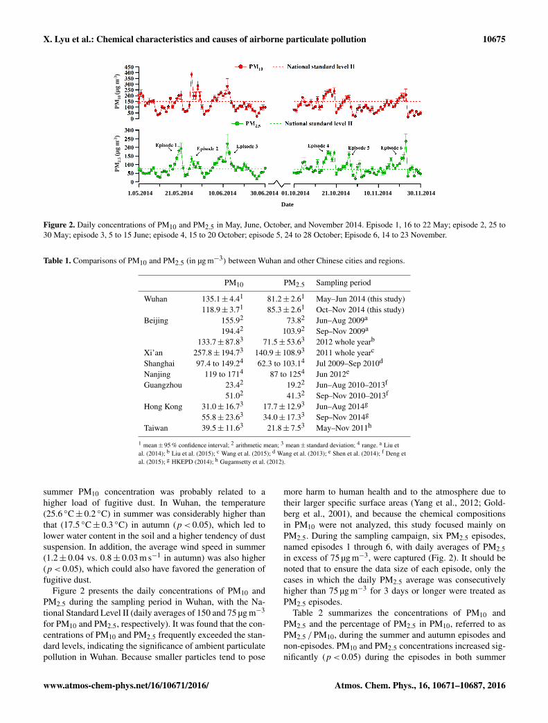
Figure 2. Daily concentrations of PM10 and PM2.5 in May, June, October, and November 2014. Episode 1, 16 to 22 May; episode 2, 25 to30 May; episode 3, 5 to 15 June; episode 4, 15 to 20 October; episode 5, 24 to 28 October; Episode 6, 14 to 23 November.

Table 1. Comparisons of PM10 and PM2.5 (in µg m−3) between Wuhan and other Chinese cities and regions.

PM10 PM2.5 Sampling period

Wuhan 135.1± 4.41 81.2± 2.61 May–Jun 2014 (this study)118.9± 3.71 85.3± 2.61 Oct–Nov 2014 (this study)

Beijing 155.92 73.82 Jun–Aug 2009a

194.42 103.92 Sep–Nov 2009a

133.7± 87.83 71.5± 53.63 2012 whole yearb

Xi’an 257.8± 194.73 140.9± 108.93 2011 whole yearc

Shanghai 97.4 to 149.24 62.3 to 103.14 Jul 2009–Sep 2010d

Nanjing 119 to 1714 87 to 1254 Jun 2012e

Guangzhou 23.42 19.22 Jun–Aug 2010–2013f

51.02 41.32 Sep–Nov 2010–2013f

Hong Kong 31.0± 16.73 17.7± 12.93 Jun–Aug 2014g

55.8± 23.63 34.0± 17.33 Sep–Nov 2014g

Taiwan 39.5± 11.63 21.8± 7.53 May–Nov 2011h

1 mean± 95 % confidence interval; 2 arithmetic mean; 3 mean± standard deviation; 4 range. a Liu etal. (2014); b Liu et al. (2015); c Wang et al. (2015); d Wang et al. (2013); e Shen et al. (2014); f Deng etal. (2015); g HKEPD (2014); h Gugamsetty et al. (2012).

summer PM10 concentration was probably related to ahigher load of fugitive dust. In Wuhan, the temperature(25.6 ◦C± 0.2 ◦C) in summer was considerably higher thanthat (17.5 ◦C± 0.3 ◦C) in autumn (p< 0.05), which led tolower water content in the soil and a higher tendency of dustsuspension. In addition, the average wind speed in summer(1.2± 0.04 vs. 0.8± 0.03 m s−1 in autumn) was also higher(p< 0.05), which could also have favored the generation offugitive dust.

Figure 2 presents the daily concentrations of PM10 andPM2.5 during the sampling period in Wuhan, with the Na-tional Standard Level II (daily averages of 150 and 75 µg m−3

for PM10 and PM2.5, respectively). It was found that the con-centrations of PM10 and PM2.5 frequently exceeded the stan-dard levels, indicating the significance of ambient particulatepollution in Wuhan. Because smaller particles tend to pose

more harm to human health and to the atmosphere due totheir larger specific surface areas (Yang et al., 2012; Gold-berg et al., 2001), and because the chemical compositionsin PM10 were not analyzed, this study focused mainly onPM2.5. During the sampling campaign, six PM2.5 episodes,named episodes 1 through 6, with daily averages of PM2.5in excess of 75 µg m−3, were captured (Fig. 2). It should benoted that to ensure the data size of each episode, only thecases in which the daily PM2.5 average was consecutivelyhigher than 75 µg m−3 for 3 days or longer were treated asPM2.5 episodes.

Table 2 summarizes the concentrations of PM10 andPM2.5 and the percentage of PM2.5 in PM10, referred to asPM2.5 /PM10, during the summer and autumn episodes andnon-episodes. PM10 and PM2.5 concentrations increased sig-nificantly (p< 0.05) during the episodes in both summer



Table 2. Mean PM10, PM2.5, and PM2.5 /PM10 with 95 % CI dur-ing PM2.5 episodes and non-episodes in Wuhan. Non-episode 1 andNon-episode 2 represent the non-episode periods in summer and au-tumn, respectively. The values during non-episodes were in bold tofacilitate comparison.

PM10 PM2.5 PM2.5 /PM10(µg m−3) (µg m−3) (%)

Episode 1 154.3± 10.1 123.0± 9.1 72.8± 2.6Episode 2 230.1± 19.1 98.9± 5.7 45.9± 2.5Episode 3 191.4± 9.8 126.7± 7.0 66.9± 1.8Non-episode 1 98.5± 3.9 56.6± 1.7 58.9± 1.5Episode 4 221.8± 8.9 148.6± 5.2 67.9± 2.0Episode 5 154.2± 10.4 108.2± 6.8 69.3± 3.1Episode 6 157.3± 9.0 120.0± 7.6 71.2± 2.1Non-episode 2 88.7± 3.4 64.2± 2.2 65.3± 1.3

and autumn. The PM2.5 /PM10 value also increased remark-ably on episode days compared to that on non-episode days,except for episode 2 (45.9 %± 2.5 %), which suggests thatmore secondary species and/or primary fine particles (e.g.,primary OC and EC generated from combustion) were gen-erated or released during the episodes. In contrast, the lowerPM2.5 /PM10 value during episode 2 might imply a strongsource of coarse particles. Indeed, this inference was con-firmed by the source apportionment analysis in Sect. 3.3.3.

3.2 Chemical composition of PM2.5

Figure 3 shows the daily variations of PM2.5 and its composi-tion. As the instrument for the analysis of WSIs was initiallydeployed in September 2014, data are not available for Mayand June. The carbonaceous aerosol (18.5± 1.2 µg m−3) andelements (6.0± 0.3 µg m−3) accounted for 19.1 %± 0.6 %and 6.2 %± 0.2 % of PM2.5 in summer, respectively. Inautumn, WSIs were the most abundant component inPM2.5 (64.4± 2.5 µg m−3; 68.6 %± 1.9 %), followed bycarbonaceous aerosol (24.3± 1.0 µg m−3; 25.5 %± 0.8 %)and elements (4.5± 0.2 µg m−3; 4.6 %± 0.1 %). The sec-ondary inorganic ions SO2−

4 (18.8± 0.6 µg m−3), NO−3(18.7± 0.8 µg m−3), and NH+4 (12.0± 0.4 µg m−3) dom-inated the WSIs, with the average contribution of34.0 %± 0.6 %, 30.1 %± 0.5 %, and 20.4 %± 0.1 %, respec-tively.

The charge balance between the anions and cations wasusually used to predict the existing forms of SIAs and theacidity of PM2.5. Figure 4 shows the relative abundance ofmolar charges of SIAs, which were located fairly close to theone-to-one line on both episode and non-episode days. Thisfinding suggests that NH4NO3 and (NH4)2SO4 were coex-isting forms of the SIAs in PM2.5 in Wuhan. When extend-ing NH+4 to total cations (NH+4 , Ca2+, Mg2+, Na+, and K+)and NO−3 and SO2−

4 to total anions (NO−3 , SO2−4 , and Cl−),

the molar charges of the cations and anions were balanced

(slope, 0.98; R2= 0.98), as shown in Fig. S6 in the Supple-

ment, indicating that PM2.5 was neutralized during autumnin Wuhan.

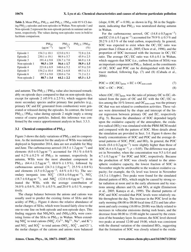
For the carbonaceous aerosol, OC (14.8± 0.5 µg m−3)

and EC (3.6± 0.1 µg m−3) accounted for 79.9 %± 0.3 % and20.2 %± 0.3 % of the total carbon, respectively. In general,SOC was expected to exist when the OC /EC ratio wasgreater than 2 (Duan et al., 2005; Chow et al., 1996), and theproportion of SOC increased with the increase in OC /ECratio. The average OC /EC ratio was 4.8± 0.1 in Wuhan,which suggests that SOC (i.e., carbon fraction of SOA) wasan important component in PM2.5. Indeed, as the constituentsof OC, SOC and POC can be distinguished with the EC-tracer method, following Eqs. (7) and (8) (Cabada et al.,2004):

POC= (OC/EC)prim×EC+OCnon-comb (7)SOC= OC−POC, (8)

where (OC /EC)prim was the ratio of primary OC to EC, ob-tained from the pairs of OC and EC with the OC /EC ra-tios among the 10 % lowest; and OCnon-comb was the primaryOC that was not related to combustion activities. These val-ues were determined by the slope and intercept of the lin-ear regression between primary OC and EC, respectively(Fig. 5). Because the abundance of SOC depended largelyupon the oxidative capacity of the atmosphere, the oxida-tive radical (HO2)was simulated with the PBM-MCM modeland compared with the pattern of SOC. More details aboutthe simulation are provided in Sect. 3.4. Figure 6 shows thehourly concentrations of SOC and POC and the average di-urnal patterns of SOC, POC, and HO2. In general, the POClevels (8.6± 0.2 µg m−3) were slightly higher than those ofSOC (6.4± 0.3 µg m−3; p< 0.05). The difference was great-est in November, when the concentration was 9.5± 0.4 and4.7± 0.3 µg m−3 for POC and SOC, respectively. Becausethe production of SOC was closely related to the atmo-spheric oxidative capacity, the lowest fraction of SOC inNovember might be attributable to the weakest oxidative ca-pacity; for example, the O3 level was lowest in November(14.3± 1.0 ppbv). Two peaks were found for the simulateddiurnal pattern of HO2, which might be caused by strong so-lar radiation at noon and in the early afternoon and by reac-tions among alkenes and O3 and NO3 at night (Emmersonet al., 2005; Kanaya et al., 1999). The diurnal patterns ofPOC and SOC revealed that POC levels were relatively sta-ble throughout the day. The increase in the POC level in theearly morning (06:00 to 08:00 local time (LT)) and late after-noon and early evening (16:00 to 20:00) was likely related toincreases in vehicular emissions during rush hours, and thedecrease from 08:00 to 15:00 might be caused by the exten-sion of the boundary layer. In contrast, the SOC level showedtwo peaks at around 12:00 and 19:00, which was consistentwith the diurnal variation of the simulated HO2, suggestingthat the formation of SOC was closely related to the oxida-



Con

cent

ratio

n (µ

g m

)-3

Me

Figure 3. Daily variations of PM2.5 and its components. Pie charts represent the composition of elements and water-soluble ions, respectively.Pink shaded areas represent episodes.

Non-episodeEpisode

One-to-one line

(µmol m )-3

(µm

ol m

)-3

Figure 4. Relative abundance of molar charges of PM2.5 duringautumn in Wuhan.

tive radicals in the atmosphere. (A detailed relationship isdiscussed in Sect. 3.4.3.)

Among the elements, potassium (K;2060.7± 82.3 ng m−3), iron (Fe; 996.5± 34.3 ng m−3),and calcium (Ca; 774.1± 39.4 ng m−3) were the most abun-dant species, accounting for 47.0 %± 2.2 %, 21.4 %± 0.3 %,and 15.6 %± 0.3 % of the total analyzed elements, respec-tively. Correlation analysis indicated that Fe had goodcorrelation with Ca (R2

= 0.66; Fig. S7 in the Supplement),whereas weak correlations of K with Fe (R2

= 0.14) and Ca(R2= 0.09) were found, suggesting that Fe and Ca shared

common sources that were different from the sources of K.Because Fe and Ca are typical crustal elements, fugitivedust (e.g., dust from traffic, construction and demolitionworks, yards, and bare soil) was their most likely source. Incontrast, apart from emissions from mineral sources, K isalso emitted from biomass burning. As such, K was believedto be mainly emitted from biomass burning in this study,

which is further supported by the moderate correlations of Kwith OC (R2

= 0.52) and EC (R2= 0.48) because biomass

burning also emits OC and EC (Saarikoski et al., 2007;Echalar et al., 1995).

3.3 Causes of PM2.5 episodes

3.3.1 Meteorological conditions

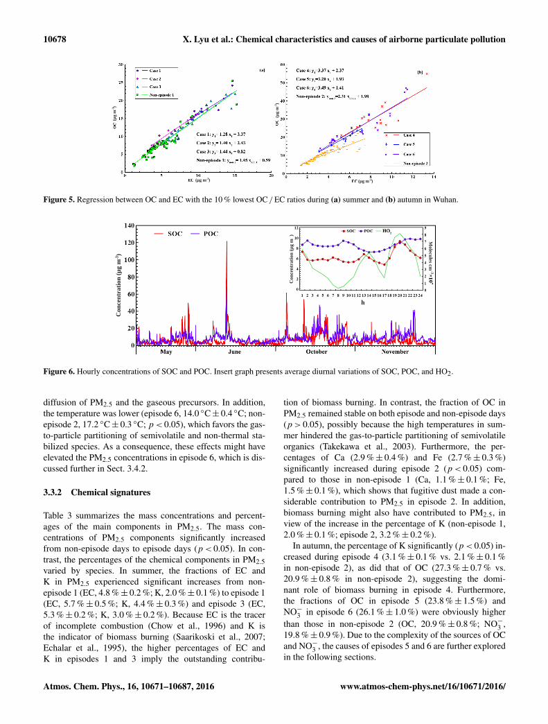
The processes of particle formation, dispersion, and de-position are closely related to meteorological conditions.To interpret the possible causes of the PM2.5 episodes,Fig. 7 shows the patterns of wind direction and speed,temperature, relative humidity, and atmospheric pressure inWuhan during the monitoring period. In general, southeastwinds prevailed at the sampling site with a wind speedof approximately 1.0 m s−1. The low wind speed indicatesthe dominance of local air masses. However, due to thehigh stability and long lifetime of PM2.5, the regional andsuper-regional impact could not be eliminated. In com-parison with those in summer, the wind speed (summer,1.1± 0.04 m s−1; autumn, 0.8± 0.03 m s−1) and tempera-ture (summer, 25.6± 0.2 m s−1; autumn, 17.5± 0.3 m s−1)were significantly (p< 0.05) lower in autumn, whereas theatmospheric pressure (summer, 1006.9< 0.2 hPa; autumn,1020.9± 0.2 hPa) was much higher. During the episodes, thewind speed was generally lower than during non-episodes,with the exception of episode 5. This might be one cause forthe episodes, but it does not fully explain the great enhance-ments of PM2.5, because the wind speeds were very lowand the differences between the episodes and non-episodeswere minor. The atmospheric pressure was not very high dur-ing episodes 1 through 5, suggesting that the synoptic sys-tem was not responsible for the occurrence of these PM2.5episodes. However, the atmospheric pressure was remarkablyhigher (p< 0.05) in episode 6 (1024± 1 hPa) than in non-episode 2 (1021± 0.3 hPa), which might have suppressed the



(µg

m )-3

(µg

m )-3

(µg m )-3 (µg m )-3

Figure 5. Regression between OC and EC with the 10 % lowest OC /EC ratios during (a) summer and (b) autumn in Wuhan.

Con

cent

ratio

n (µ

g m

)-3

Con

cent

ratio

n (µ

g m

) Molecules cm

-3

h

Figure 6. Hourly concentrations of SOC and POC. Insert graph presents average diurnal variations of SOC, POC, and HO2.

diffusion of PM2.5 and the gaseous precursors. In addition,the temperature was lower (episode 6, 14.0 ◦C± 0.4 ◦C; non-episode 2, 17.2 ◦C± 0.3 ◦C; p< 0.05), which favors the gas-to-particle partitioning of semivolatile and non-thermal sta-bilized species. As a consequence, these effects might haveelevated the PM2.5 concentrations in episode 6, which is dis-cussed further in Sect. 3.4.2.

3.3.2 Chemical signatures

Table 3 summarizes the mass concentrations and percent-ages of the main components in PM2.5. The mass con-centrations of PM2.5 components significantly increasedfrom non-episode days to episode days (p< 0.05). In con-trast, the percentages of the chemical components in PM2.5varied by species. In summer, the fractions of EC andK in PM2.5 experienced significant increases from non-episode 1 (EC, 4.8 %± 0.2 %; K, 2.0 %± 0.1 %) to episode 1(EC, 5.7 %± 0.5 %; K, 4.4 %± 0.3 %) and episode 3 (EC,5.3 %± 0.2 %; K, 3.0 %± 0.2 %). Because EC is the tracerof incomplete combustion (Chow et al., 1996) and K isthe indicator of biomass burning (Saarikoski et al., 2007;Echalar et al., 1995), the higher percentages of EC andK in episodes 1 and 3 imply the outstanding contribu-

tion of biomass burning. In contrast, the fraction of OC inPM2.5 remained stable on both episode and non-episode days(p> 0.05), possibly because the high temperatures in sum-mer hindered the gas-to-particle partitioning of semivolatileorganics (Takekawa et al., 2003). Furthermore, the per-centages of Ca (2.9 %± 0.4 %) and Fe (2.7 %± 0.3 %)significantly increased during episode 2 (p< 0.05) com-pared to those in non-episode 1 (Ca, 1.1 %± 0.1 %; Fe,1.5 %± 0.1 %), which shows that fugitive dust made a con-siderable contribution to PM2.5 in episode 2. In addition,biomass burning might also have contributed to PM2.5, inview of the increase in the percentage of K (non-episode 1,2.0 %± 0.1 %; episode 2, 3.2 %± 0.2 %).

In autumn, the percentage of K significantly (p< 0.05) in-creased during episode 4 (3.1 %± 0.1 % vs. 2.1 %± 0.1 %in non-episode 2), as did that of OC (27.3 %± 0.7 % vs.20.9 %± 0.8 % in non-episode 2), suggesting the domi-nant role of biomass burning in episode 4. Furthermore,the fractions of OC in episode 5 (23.8 %± 1.5 %) andNO−3 in episode 6 (26.1 %± 1.0 %) were obviously higherthan those in non-episode 2 (OC, 20.9 %± 0.8 %; NO−3 ,19.8 %± 0.9 %). Due to the complexity of the sources of OCand NO−3 , the causes of episodes 5 and 6 are further exploredin the following sections.



DateDate

Pres

s./h

Pa

R

H/%

Tem

p./

C

Wd

and

ws

º

Pres

s./h

Pa

R

H/%

Tem

p./

C

Wd

and

ws

º

Figure 7. Meteorological patterns in Wuhan during the monitoring period. Pink shaded areas represent PM2.5 episodes.

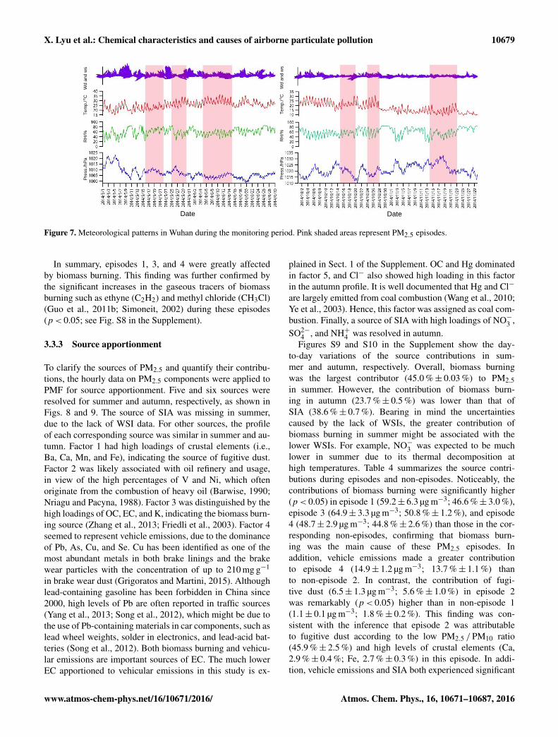
In summary, episodes 1, 3, and 4 were greatly affectedby biomass burning. This finding was further confirmed bythe significant increases in the gaseous tracers of biomassburning such as ethyne (C2H2) and methyl chloride (CH3Cl)(Guo et al., 2011b; Simoneit, 2002) during these episodes(p< 0.05; see Fig. S8 in the Supplement).

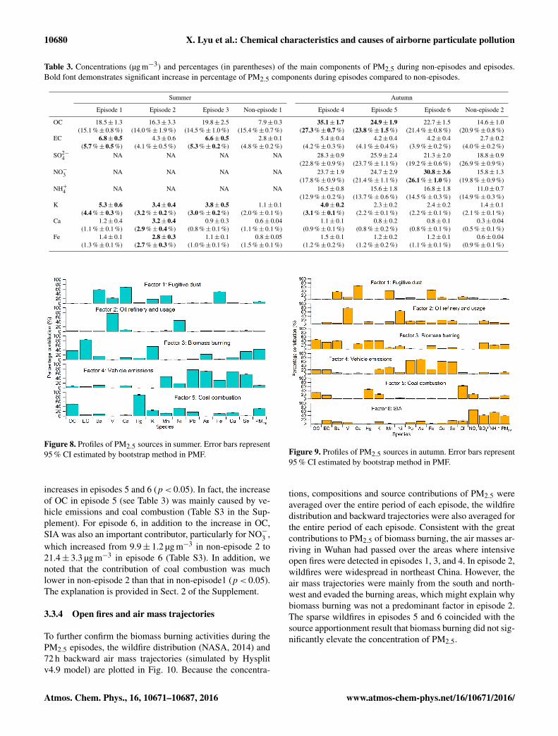
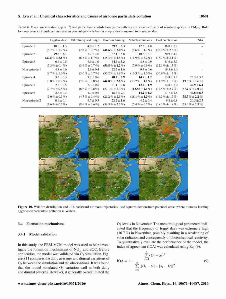
3.3.3 Source apportionment

To clarify the sources of PM2.5 and quantify their contribu-tions, the hourly data on PM2.5 components were applied toPMF for source apportionment. Five and six sources wereresolved for summer and autumn, respectively, as shown inFigs. 8 and 9. The source of SIA was missing in summer,due to the lack of WSI data. For other sources, the profileof each corresponding source was similar in summer and au-tumn. Factor 1 had high loadings of crustal elements (i.e.,Ba, Ca, Mn, and Fe), indicating the source of fugitive dust.Factor 2 was likely associated with oil refinery and usage,in view of the high percentages of V and Ni, which oftenoriginate from the combustion of heavy oil (Barwise, 1990;Nriagu and Pacyna, 1988). Factor 3 was distinguished by thehigh loadings of OC, EC, and K, indicating the biomass burn-ing source (Zhang et al., 2013; Friedli et al., 2003). Factor 4seemed to represent vehicle emissions, due to the dominanceof Pb, As, Cu, and Se. Cu has been identified as one of themost abundant metals in both brake linings and the brakewear particles with the concentration of up to 210 mg g−1

in brake wear dust (Grigoratos and Martini, 2015). Althoughlead-containing gasoline has been forbidden in China since2000, high levels of Pb are often reported in traffic sources(Yang et al., 2013; Song et al., 2012), which might be due tothe use of Pb-containing materials in car components, such aslead wheel weights, solder in electronics, and lead-acid bat-teries (Song et al., 2012). Both biomass burning and vehicu-lar emissions are important sources of EC. The much lowerEC apportioned to vehicular emissions in this study is ex-

plained in Sect. 1 of the Supplement. OC and Hg dominatedin factor 5, and Cl− also showed high loading in this factorin the autumn profile. It is well documented that Hg and Cl−

are largely emitted from coal combustion (Wang et al., 2010;Ye et al., 2003). Hence, this factor was assigned as coal com-bustion. Finally, a source of SIA with high loadings of NO−3 ,SO2−

4 , and NH+4 was resolved in autumn.Figures S9 and S10 in the Supplement show the day-

to-day variations of the source contributions in sum-mer and autumn, respectively. Overall, biomass burningwas the largest contributor (45.0 %± 0.03 %) to PM2.5in summer. However, the contribution of biomass burn-ing in autumn (23.7 %± 0.5 %) was lower than that ofSIA (38.6 %± 0.7 %). Bearing in mind the uncertaintiescaused by the lack of WSIs, the greater contribution ofbiomass burning in summer might be associated with thelower WSIs. For example, NO−3 was expected to be muchlower in summer due to its thermal decomposition athigh temperatures. Table 4 summarizes the source contri-butions during episodes and non-episodes. Noticeably, thecontributions of biomass burning were significantly higher(p< 0.05) in episode 1 (59.2± 6.3 µg m−3; 46.6 %± 3.0 %),episode 3 (64.9± 3.3 µg m−3; 50.8 %± 1.2 %), and episode4 (48.7± 2.9 µg m−3; 44.8 %± 2.6 %) than those in the cor-responding non-episodes, confirming that biomass burn-ing was the main cause of these PM2.5 episodes. Inaddition, vehicle emissions made a greater contributionto episode 4 (14.9± 1.2 µg m−3; 13.7 %± 1.1 %) thanto non-episode 2. In contrast, the contribution of fugi-tive dust (6.5± 1.3 µg m−3; 5.6 %± 1.0 %) in episode 2was remarkably (p< 0.05) higher than in non-episode 1(1.1± 0.1 µg m−3; 1.8 %± 0.2 %). This finding was con-sistent with the inference that episode 2 was attributableto fugitive dust according to the low PM2.5 /PM10 ratio(45.9 %± 2.5 %) and high levels of crustal elements (Ca,2.9 %± 0.4 %; Fe, 2.7 %± 0.3 %) in this episode. In addi-tion, vehicle emissions and SIA both experienced significant



Table 3. Concentrations (µg m−3) and percentages (in parentheses) of the main components of PM2.5 during non-episodes and episodes.Bold font demonstrates significant increase in percentage of PM2.5 components during episodes compared to non-episodes.

Summer Autumn

Episode 1 Episode 2 Episode 3 Non-episode 1 Episode 4 Episode 5 Episode 6 Non-episode 2

OC 18.5± 1.3 16.3± 3.3 19.8± 2.5 7.9± 0.3 35.1± 1.7 24.9± 1.9 22.7± 1.5 14.6± 1.0(15.1 %± 0.8 %) (14.0 %± 1.9 %) (14.5 %± 1.0 %) (15.4 %± 0.7 %) (27.3 %± 0.7 %) (23.8 %± 1.5 %) (21.4 %± 0.8 %) (20.9 %± 0.8 %)

EC 6.8± 0.5 4.3± 0.6 6.6± 0.5 2.8± 0.1 5.4± 0.4 4.2± 0.4 4.2± 0.4 2.7± 0.2(5.7 %± 0.5 %) (4.1 %± 0.5 %) (5.3 %± 0.2 %) (4.8 %± 0.2 %) (4.2 %± 0.3 %) (4.1 %± 0.4 %) (3.9 %± 0.2 %) (4.0 %± 0.2 %)

SO2−4 NA NA NA NA 28.3± 0.9 25.9± 2.4 21.3± 2.0 18.8± 0.9

(22.8 %± 0.9 %) (23.7 %± 1.1 %) (19.2 %± 0.6 %) (26.9 %± 0.9 %)NO−3 NA NA NA NA 23.7± 1.9 24.7± 2.9 30.8± 3.6 15.8± 1.3

(17.8 %± 0.9 %) (21.4 %± 1.1 %) (26.1 %± 1.0 %) (19.8 %± 0.9 %)NH+4 NA NA NA NA 16.5± 0.8 15.6± 1.8 16.8± 1.8 11.0± 0.7

(12.9 %± 0.2 %) (13.7 %± 0.6 %) (14.5 %± 0.3 %) (14.9 %± 0.3 %)K 5.3± 0.6 3.4± 0.4 3.8± 0.5 1.1± 0.1 4.0± 0.2 2.3± 0.2 2.4± 0.2 1.4± 0.1

(4.4 %± 0.3 %) (3.2 %± 0.2 %) (3.0 %± 0.2 %) (2.0 %± 0.1 %) (3.1 %± 0.1 %) (2.2 %± 0.1 %) (2.2 %± 0.1 %) (2.1 %± 0.1 %)Ca 1.2± 0.4 3.2± 0.4 0.9± 0.3 0.6± 0.04 1.1± 0.1 0.8± 0.2 0.8± 0.1 0.3± 0.04

(1.1 %± 0.1 %) (2.9 %± 0.4 %) (0.8 %± 0.1 %) (1.1 %± 0.1 %) (0.9 %± 0.1 %) (0.8 %± 0.2 %) (0.8 %± 0.1 %) (0.5 %± 0.1 %)Fe 1.4± 0.1 2.8± 0.3 1.1± 0.1 0.8± 0.05 1.5± 0.1 1.2± 0.2 1.2± 0.1 0.6± 0.04

(1.3 %± 0.1 %) (2.7 %± 0.3 %) (1.0 %± 0.1 %) (1.5 %± 0.1 %) (1.2 %± 0.2 %) (1.2 %± 0.2 %) (1.1 %± 0.1 %) (0.9 %± 0.1 %)

Figure 8. Profiles of PM2.5 sources in summer. Error bars represent95 % CI estimated by bootstrap method in PMF.

increases in episodes 5 and 6 (p< 0.05). In fact, the increaseof OC in episode 5 (see Table 3) was mainly caused by ve-hicle emissions and coal combustion (Table S3 in the Sup-plement). For episode 6, in addition to the increase in OC,SIA was also an important contributor, particularly for NO−3 ,which increased from 9.9± 1.2 µg m−3 in non-episode 2 to21.4± 3.3 µg m−3 in episode 6 (Table S3). In addition, wenoted that the contribution of coal combustion was muchlower in non-episode 2 than that in non-episode1 (p< 0.05).The explanation is provided in Sect. 2 of the Supplement.

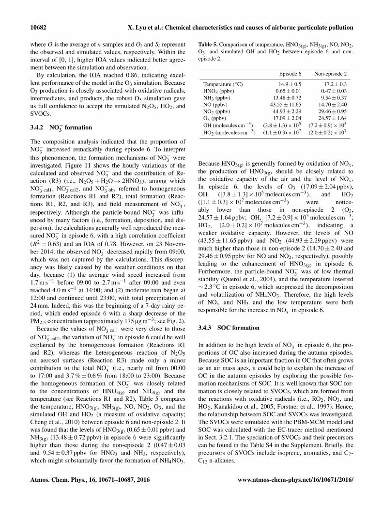
3.3.4 Open fires and air mass trajectories

To further confirm the biomass burning activities during thePM2.5 episodes, the wildfire distribution (NASA, 2014) and72 h backward air mass trajectories (simulated by Hysplitv4.9 model) are plotted in Fig. 10. Because the concentra-

Figure 9. Profiles of PM2.5 sources in autumn. Error bars represent95 % CI estimated by bootstrap method in PMF.

tions, compositions and source contributions of PM2.5 wereaveraged over the entire period of each episode, the wildfiredistribution and backward trajectories were also averaged forthe entire period of each episode. Consistent with the greatcontributions to PM2.5 of biomass burning, the air masses ar-riving in Wuhan had passed over the areas where intensiveopen fires were detected in episodes 1, 3, and 4. In episode 2,wildfires were widespread in northeast China. However, theair mass trajectories were mainly from the south and north-west and evaded the burning areas, which might explain whybiomass burning was not a predominant factor in episode 2.The sparse wildfires in episodes 5 and 6 coincided with thesource apportionment result that biomass burning did not sig-nificantly elevate the concentration of PM2.5.



Table 4. Mass concentration (µg m−3) and percentage contribution (in parentheses) of sources to sum of resolved species in PM2.5. Boldfont represents a significant increase in percentage contribution in episodes compared to non-episodes.

Fugitive dust Oil refinery and usage Biomass burning Vehicle emissions Coal combustion SIA

Episode 1 10.0± 1.3 4.0± 1.2 59.2± 6.3 12.2± 1.8 36.0± 2.7 –(8.7 %± 1.2 %) (2.8 %± 0.7 %) (46.6 %± 3.0 %) (9.6 %± 1.2 %) (32.2 %± 2.5 %)

Episode 2 29.5± 6.1 8.2± 2.6 37.1± 5.8 10.8± 3.1 20.9± 4.7 –(27.5 %± 5.5 %) (6.7 %± 1.7 %) (35.3 %± 4.8 %) (11.9 %± 3.2 %) (18.7 %± 3.1 %)

Episode 3 6.4± 0.5 4.9± 1.0 64.9± 3.3 8.8± 0.9 41.6± 3.3 –(5.3 %± 0.4 %) (3.9 %± 0.7 %) (50.8 %± 1.2 %) (7.9 %± 0.9 %) (32.1 %± 1.5 %)

Non-episode 1 4.8± 0.6 2.9± 0.4 22.2± 1.6 9.3± 0.6 19.5± 1.0 –(8.7 %± 1.0 %) (5.0 %± 0.7 %) (35.2 %± 1.9 %) (16.3 %± 1.0 %) (35.9 %± 1.7 %)

Episode 4 3.3± 0.3 7.2± 0.6 48.7± 2.9 14.9± 1.2 13.8± 1.7 23.3± 3.3(3.0 %± 0.2 %) (7.0 %± 0.8 %) (44.8 %± 2.6 %) (13.7 %± 1.1 %) (11.9 %± 1.3 %) (19.6 %± 2.6 %)

Episode 5 2.3± 0.5 5.3± 0.6 21.1± 2.8 12.2± 1.9 14.8± 2.0 39.9± 6.4(2.7 %± 0.5 %) (6.6 %± 0.8 %) (22.1 %± 2.3 %) (13.85± 2.1 %) (17.5 %± 2.7 %) (37.2 %± 3.0 %)

Episode 6 2.6± 0.3 4.7± 0.6 18.4± 2.4 14.2± 1.3 17.7± 2.5 44.6± 6.8(3.0 %± 0.3 %) (4.7 %± 0.4 %) (21.2 %± 2.5 %) (16.1 %± 1.3 %) (16.3 %± 1.7 %) (38.7 %± 2.2 %)

Non-episode 2 0.9± 0.1 4.7± 0.3 22.2± 1.6 4.2± 0.4 9.8± 0.8 20.5± 2.5(1.6 %± 0.2 %) (8.6 %± 0.6 %) (39.3 %± 2.5 %) (7.4 %± 0.7 %) (18.1 %± 1.8 %) (25.0 %± 2.3 %)

Figure 10. Wildfire distribution and 72 h backward air mass trajectories. Red squares demonstrate potential areas where biomass burningaggravated particulate pollution in Wuhan.

3.4 Formation mechanisms

3.4.1 Model validation

In this study, the PBM-MCM model was used to help inves-tigate the formation mechanisms of NO−3 and SOC. Beforeapplication, the model was validated via O3 simulation. Fig-ure S11 compares the daily averages and diurnal variations ofO3 between the simulation and the observations. It was foundthat the model simulated O3 variation well in both dailyand diurnal patterns. However, it generally overestimated the

O3 levels in November. The meteorological parameters indi-cated that the frequency of foggy days was extremely high(36.7 %) in November, possibly resulting in a weakening ofsolar radiation and consequently of photochemical reactivity.To quantitatively evaluate the performance of the model, theindex of agreement (IOA) was calculated using Eq. (9).

IOA= 1−

n∑i=1(Oi − Si)

2

n∑i=1(|Oi − O| + |Si − O|)2

, (9)



where O is the average of n samples andOi and Si representthe observed and simulated values, respectively. Within theinterval of [0, 1], higher IOA values indicated better agree-ment between the simulation and observation.

By calculation, the IOA reached 0.86, indicating excel-lent performance of the model in the O3 simulation. BecauseO3 production is closely associated with oxidative radicals,intermediates, and products, the robust O3 simulation gaveus full confidence to accept the simulated N2O5, HO2, andSVOCs.

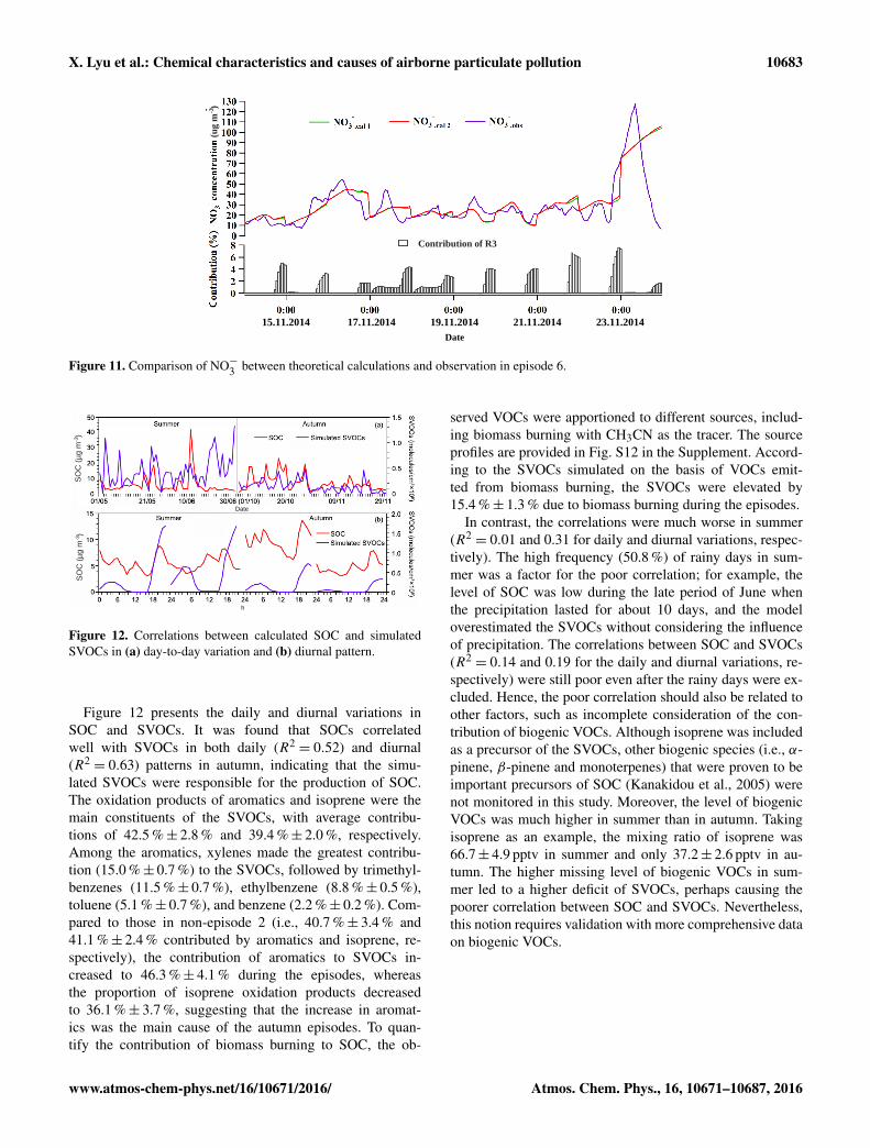
3.4.2 NO−3 formation

The composition analysis indicated that the proportion ofNO−3 increased remarkably during episode 6. To interpretthis phenomenon, the formation mechanisms of NO−3 wereinvestigated. Figure 11 shows the hourly variations of thecalculated and observed NO−3 and the contribution of Re-action (R3) (i.e., N2O5+H2O→ 2HNO3), among whichNO−3 cal1, NO−3 cal2, and NO−3 obs referred to homogeneousformation (Reactions R1 and R2), total formation (Reac-tions R1, R2, and R3), and field measurement of NO−3 ,respectively. Although the particle-bound NO−3 was influ-enced by many factors (i.e., formation, deposition, and dis-persion), the calculations generally well reproduced the mea-sured NO−3 in episode 6, with a high correlation coefficient(R2= 0.63) and an IOA of 0.78. However, on 23 Novem-

ber 2014, the observed NO−3 decreased rapidly from 09:00,which was not captured by the calculations. This discrep-ancy was likely caused by the weather conditions on thatday, because (1) the average wind speed increased from1.7 m s−1 before 09:00 to 2.7 m s−1 after 09:00 and evenreached 4.0 m s−1 at 14:00; and (2) moderate rain began at12:00 and continued until 23:00, with total precipitation of24 mm. Indeed, this was the beginning of a 7-day rainy pe-riod, which ended episode 6 with a sharp decrease of thePM2.5 concentration (approximately 175 µg m−3; see Fig. 2).

Because the values of NO−3 cal1 were very close to thoseof NO−3 cal2, the variation of NO−3 in episode 6 could be wellexplained by the homogeneous formation (Reactions R1and R2), whereas the heterogeneous reaction of N2O5on aerosol surfaces (Reaction R3) made only a minorcontribution to the total NO−3 (i.e., nearly nil from 00:00to 17:00 and 3.7 %± 0.6 % from 18:00 to 23:00). Becausethe homogeneous formation of NO−3 was closely relatedto the concentrations of HNO3(g) and NH3(g) and thetemperature (see Reactions R1 and R2), Table 5 comparesthe temperature, HNO3(g), NH3(g), NO, NO2, O3, and thesimulated OH and HO2 (a measure of oxidative capacity;Cheng et al., 2010) between episode 6 and non-episode 2. Itwas found that the levels of HNO3(g) (0.65± 0.01 ppbv) andNH3(g) (13.48± 0.72 ppbv) in episode 6 were significantlyhigher than those during the non-episode 2 (0.47± 0.03and 9.54± 0.37 ppbv for HNO3 and NH3, respectively),which might substantially favor the formation of NH4NO3.

Table 5. Comparison of temperature, HNO3(g), NH3(g), NO, NO2,O3, and simulated OH and HO2 between episode 6 and non-episode 2.

Episode 6 Non-episode 2

Temperature (◦C) 14.9± 0.5 17.2± 0.3HNO3 (ppbv) 0.65± 0.01 0.47± 0.03NH3 (ppbv) 13.48± 0.72 9.54± 0.37NO (ppbv) 43.55± 11.65 14.70± 2.40NO2 (ppbv) 44.93± 2.29 29.46± 0.95O3 (ppbv) 17.09± 2.04 24.57± 1.64OH (molecules cm−3) (3.8± 1.3)× 105 (7.2± 0.9)× 105

HO2 (molecules cm−3) (1.1± 0.3)× 107 (2.0± 0.2)× 107

Because HNO3(g) is generally formed by oxidation of NOx ,the production of HNO3(g) should be closely related tothe oxidative capacity of the air and the level of NOx .In episode 6, the levels of O3 (17.09± 2.04 ppbv),OH ([3.8± 1.3]× 105 molecules cm−3), and HO2([1.1± 0.3]× 107 molecules cm−3) were notice-ably lower than those in non-episode 2 (O3,24.57± 1.64 ppbv; OH, [7.2± 0.9]× 105 molecules cm−3;HO2, [2.0± 0.2]× 107 molecules cm−3), indicating aweaker oxidative capacity. However, the levels of NO(43.55± 11.65 ppbv) and NO2 (44.93± 2.29 ppbv) weremuch higher than those in non-episode 2 (14.70± 2.40 and29.46± 0.95 ppbv for NO and NO2, respectively), possiblyleading to the enhancement of HNO3(g) in episode 6.Furthermore, the particle-bound NO−3 was of low thermalstability (Querol et al., 2004), and the temperature lowered∼ 2.3 ◦C in episode 6, which suppressed the decompositionand volatilization of NH4NO3. Therefore, the high levelsof NOx and NH3 and the low temperature were bothresponsible for the increase in NO−3 in episode 6.

3.4.3 SOC formation

In addition to the high levels of NO−3 in episode 6, the pro-portions of OC also increased during the autumn episodes.Because SOC is an important fraction in OC that often growsas an air mass ages, it could help to explain the increase ofOC in the autumn episodes by exploring the possible for-mation mechanisms of SOC. It is well known that SOC for-mation is closely related to SVOCs, which are formed fromthe reactions with oxidative radicals (i.e., RO2, NO3, andHO2; Kanakidou et al., 2005; Forstner et al., 1997). Hence,the relationship between SOC and SVOCs was investigated.The SVOCs were simulated with the PBM-MCM model andSOC was calculated with the EC-tracer method mentionedin Sect. 3.2.1. The speciation of SVOCs and their precursorscan be found in the Table S4 in the Supplement. Briefly, theprecursors of SVOCs include isoprene, aromatics, and C7-C12 n-alkanes.



(ug

m )-3

15.11.2014 17.11.2014 19.11.2014 21.11.2014 23.11.2014 Date

Contribution of R3

Figure 11. Comparison of NO−3 between theoretical calculations and observation in episode 6.

Date

h

SOC

(µg

m )-3

SOC

(µg

m )-3

Figure 12. Correlations between calculated SOC and simulatedSVOCs in (a) day-to-day variation and (b) diurnal pattern.

Figure 12 presents the daily and diurnal variations inSOC and SVOCs. It was found that SOCs correlatedwell with SVOCs in both daily (R2

= 0.52) and diurnal(R2= 0.63) patterns in autumn, indicating that the simu-

lated SVOCs were responsible for the production of SOC.The oxidation products of aromatics and isoprene were themain constituents of the SVOCs, with average contribu-tions of 42.5 %± 2.8 % and 39.4 %± 2.0 %, respectively.Among the aromatics, xylenes made the greatest contribu-tion (15.0 %± 0.7 %) to the SVOCs, followed by trimethyl-benzenes (11.5 %± 0.7 %), ethylbenzene (8.8 %± 0.5 %),toluene (5.1 %± 0.7 %), and benzene (2.2 %± 0.2 %). Com-pared to those in non-episode 2 (i.e., 40.7 %± 3.4 % and41.1 %± 2.4 % contributed by aromatics and isoprene, re-spectively), the contribution of aromatics to SVOCs in-creased to 46.3 %± 4.1 % during the episodes, whereasthe proportion of isoprene oxidation products decreasedto 36.1 %± 3.7 %, suggesting that the increase in aromat-ics was the main cause of the autumn episodes. To quan-tify the contribution of biomass burning to SOC, the ob-

served VOCs were apportioned to different sources, includ-ing biomass burning with CH3CN as the tracer. The sourceprofiles are provided in Fig. S12 in the Supplement. Accord-ing to the SVOCs simulated on the basis of VOCs emit-ted from biomass burning, the SVOCs were elevated by15.4 %± 1.3 % due to biomass burning during the episodes.

In contrast, the correlations were much worse in summer(R2= 0.01 and 0.31 for daily and diurnal variations, respec-

tively). The high frequency (50.8 %) of rainy days in sum-mer was a factor for the poor correlation; for example, thelevel of SOC was low during the late period of June whenthe precipitation lasted for about 10 days, and the modeloverestimated the SVOCs without considering the influenceof precipitation. The correlations between SOC and SVOCs(R2= 0.14 and 0.19 for the daily and diurnal variations, re-

spectively) were still poor even after the rainy days were ex-cluded. Hence, the poor correlation should also be related toother factors, such as incomplete consideration of the con-tribution of biogenic VOCs. Although isoprene was includedas a precursor of the SVOCs, other biogenic species (i.e., α-pinene, β-pinene and monoterpenes) that were proven to beimportant precursors of SOC (Kanakidou et al., 2005) werenot monitored in this study. Moreover, the level of biogenicVOCs was much higher in summer than in autumn. Takingisoprene as an example, the mixing ratio of isoprene was66.7± 4.9 pptv in summer and only 37.2± 2.6 pptv in au-tumn. The higher missing level of biogenic VOCs in sum-mer led to a higher deficit of SVOCs, perhaps causing thepoorer correlation between SOC and SVOCs. Nevertheless,this notion requires validation with more comprehensive dataon biogenic VOCs.



4 Conclusions

In summer and autumn 2014, the concentrations of PM2.5and its components were continuously monitored in Wuhan;six PM2.5 episodes were captured. The analysis of PM2.5concentrations and compositions found that Wuhan sufferedfrom relatively high levels of PM2.5, even in the warm sea-sons. Secondary inorganic ions were the most predominantspecies in PM2.5 in the form of NH4NO3 and (NH4)2SO4.Comparable levels of SO2−

4 and NO−3 indicate that station-ary and mobile sources had equivalent importance in Wuhan.With the EC-tracer method, it was found that the POC levelwas slightly higher than that of SOC, and both increased sig-nificantly during the episodes. K was the most abundant el-ement in PM2.5, implying biomass burning in and aroundWuhan during the sampling campaign. Indeed, the sourceapportionment revealed that biomass burning was the maincause of increases in PM2.5 in episodes 1, 3, and 4. Fugitivedust was the leading factor in episode 2. However, episodes 5and 6 were mainly attributable to vehicle emissions andSIAs. Study of the formation mechanism of NO−3 and SOCfound that NO−3 was mainly generated from the homoge-neous reactions in episode 6, and the high levels of NOx andNH3 and the low temperature caused the increase in NO−3 .Furthermore, the daily and diurnal variations of SOC corre-lated well with those of SVOCs in autumn. Aromatics andisoprene were the main precursors of SOC, and the contri-bution of aromatics increased during the episodes. However,the correlation between SOC and SVOCs was much worsein summer, possibly as a result of the incompleteness of thebiogenic VOC input in the simulation of SVOCs. This studyadvances our understanding of the chemical characteristicsof PM2.5 in warm seasons in Wuhan and for the first timequantifies the contribution of biomass burning to PM2.5. Theinvestigation of SOC formation will also inspire the appli-cation of the explicit chemical mechanisms on the study ofSOA.

5 Data availability

The underlying research data were available at:https://drive.google.com/open?id=0BzLREyLa_fx6WjgtVW9ZaVJOd0k.

The Supplement related to this article is available onlineat doi:10.5194/acp-16-10671-2016-supplement.

Acknowledgements. This study was supported by the ResearchGrants Council of the Hong Kong Special Administrative Regionvia grants PolyU5154/13E, PolyU152052/14E, CRF/C5022-14G,and CRF/C5504-15E and the Hong Kong Polytechnic University

PhD scholarships (project #RTUP). This study is partly sup-ported by the Hong Kong PolyU internal grant (1-ZVCX and4-BCAV) and the National Natural Science Foundation of China(No. 41275122).

Edited by: X. QuerolReviewed by: four anonymous referees

References

Anderson, J. O., Thundiyil, J. G., and Stolbach, A.: Clearing theair: A review of the effects of particulate matter air pollution onhuman health, J. Med. Toxicol., 8, 166–175, 2012.

Aumont, B., Madronich, S., Ammann, M., Kalberer, M., Baltnes-perger, U., Hauglustaine, D., and Baltensperger, F.: On theNO2+ soot reaction in the atmospherem J. Geophys. Res.m 104,1729–1736, 1999.

Barwise, A. J. G.: Role of nickel and vanadium in petroleum classi-fication, Energ. Fuel., 4, 647–652, 1990.

Brown, S. G., Frankel, A., and Hafner, H. R.: Source apportionmentof VOCs in Los Angeles area using positive matrix factorization,Atmos. Environ., 41, 227–237, 2007.

Cabada, J. C., Pandis, S. N., Subramanian, R., Robinson, A. L.,Polidori, A., and Turpin, B.: Estimating the secondary organicaerosol contribution to PM2.5 using the EC tracer method,Aerosol Sci. Tech., 38, 140–155, 2004.

Cao, J. J., Wu, F., Chow, J. C., Lee, S. C., Li, Y., Chen, S. W., An, Z.S., Fung, K. K., Watson, J. G., Zhu, C. S., and Liu, S. X.: Char-acterization and source apportionment of atmospheric organicand elemental carbon during fall and winter of 2003 in Xi’an,China, Atmos. Chem. Phys., 5, 3127–3137, doi:10.5194/acp-5-3127-2005, 2005.

Cao, J. J., Shen, Z. X., Chow, J. C., Watson, J. G., Lee, S. C., Tie, X.X., Ho, K. F., Wang, G. H., and Han, Y. M.: Winter and summerPM2.5 chemical compositions in fourteen Chinese cities, J. AirWaste Manage., 62, 1214–1226, 2012.

Cheng, H. R., Guo, H., Wang, X. M., Saunders, S. M., Lam, S. H.M., Jiang, F., Wang, T. J., Ding, A. J., Lee, S. C., and Ho, K. F.:On the relationship between ozone and its precursors in the PearlRiver Delta: application of an observation-based model (OBM),Environ. Sci. Pollut. Res., 17, 547–560, 2010.

Cheng, H. R., Gong, W., Wang, Z. W., Zhang, F., Wang, X. M., Lv,X. P., Liu, J., Fu, X. X., and Zhang, G.: Ionic composition ofsubmicron particles (PM1.0) during the long-lasting haze periodin January 2013 in Wuhan, central China, J. Environ. Sci., 26,810–817, 2014.

Chow, J. C., Watson, J. G., Lu, Z. Q., Lowenthal, D. H., Frazier,C. A., Solomon, P. A., Thuillier, R. H., and Magliano, K.: De-scriptive analysis of PM2.5 and PM10 at regionally representativelocations during SJVAQS/AUSPEX, Atmos. Environ., 30, 2079–2112, 1996.

Deng, X. J., Tie, X. X., Zhou, X. J., Wu, D., Zhong, L. J., Tan, H. B.,Li, F., Huang, X. Y., Bi, X. Y., and Deng, T.: Effects of SoutheastAsia biomass burning on aerosols and ozone concentrations overthe Pearl River Delta (PRD) region, Atmos. Environ., 43, 8493–8501, 2008.


https://drive.google.com/open?id=0BzLREyLa_fx6WjgtVW9ZaVJOd0k

https://drive.google.com/open?id=0BzLREyLa_fx6WjgtVW9ZaVJOd0k

http://dx.doi.org/10.5194/acp-16-10671-2016-supplement

http://dx.doi.org/10.5194/acp-5-3127-2005



Deng, X. J., Li, F., Li, Y. H., Li, J. Y., Huang, H. Z., and Liu, X. T.:Vertical distribution characteristics of PM in the surface layer ofGuangzhou, Particuology, 20, 3–9, 2015.

Duan, F. K., He, K. B., Ma, Y. L., Jia, Y. T., Yang, F. M., Lei,Y., Tanaka, S., and Okuta, T.: Characteristics of carbonaceousaerosols in Beijing, China, Chemosphere, 60, 355–364, 2005.

Echalar, F., Gaudichet, A., Cachier, H., and Artaxo, P.: Aerosolemissions by tropical forest and savanna biomass burning: char-acteristic trace elements and fluxes, Geophys. Res. Lett., 22,3039–3042, 1995.

Emmerson, K. M., Carslaw, N., Carpenter, L. J., Heard, D. E., Lee,J. D., and Pilling, M. J.: Urban atmospheric chemistry duringthe PUMA campaign 1: Comparison of modelled OH and HO2concentrations with measurements, J. Atmos. Chem., 52, 143–164, 2005.

Forstner, H. J. L., Flagan, R. C., and Seinfeld, J. H.: Secondary or-ganic aerosol from the photooxidation of aromatic hydrocarbons:molecular composition, Environ. Sci. Technol., 31, 1345–1358,1997.

Friedli, H. R., Radke, L. F., Lu, J. Y., Banic, C. M., Leaitch, W.R., and MacPherson, J. I.: Mercury emissions from burning ofbiomass from temperate North American forests: laboratory andairborne measurements, Atmos. Environ., 37, 253–267, 2003.

GB 3095-2012: available at: http://kjs.mep.gov.cn/hjbhbz/bzwb/dqhjbh/dqhjzlbz/201203/W020120410330232398521.pdf, lastaccess: 1 August 2016.

Geng, F. H., Zhang, Q., Tie, X. X., Huang, M. Y., Ma, X. C., Deng,Z. Z., Yu, Q., Quan, J. N., and Zhao, C. S.: Aircraft measurementsof O3, NOx , CO, VOCs, and SO2 in the Yangtze River Deltaregion, Atmos. Environ., 43, 584–593, 2009.

Goldberg, M. S., Burnett, R. T., Bailar III, J. C., Brook, J., Bonva-lot, Y., Tamblyn, R., Singh, R., and Valois, M. F.: The associa-tion between daily mortality and ambient air particle pollution inMontreal, Quebec: 1. Nonaccidental mortality, Environ. Res., 86,12–25, 2001.

Grigoratos, T. and Martini, G.: Brake wear particle emissions: a re-view, Environ. Sci. Pollut. Res., 22, 2491–2504, 2015.

Gugamsetty, B., Wei, H., Liu, C. N., Awasthi, A., Hsu, S. C., Tsai,C. J, Roan, G. D., Wu, Y. C., and Chen, C. F.: Source Characteri-zation and Apportionment of PM10, PM2.5 and PM0.1 by UsingPositive Matrix Factorization, Aerosol Air Qual. Res., 12, 476–491, 2012.

Guo, H., Zou, S. C., Tsai, W. Y., Chan, L. Y., and Blake, D. R.:Emission characteristics of nonmethane hydrocarbons from pri-vate cars and taxis at different driving speeds in Hong Kong, At-mos. Environ., 45, 2711–2721, 2011a.

Guo, H., Cheng, H. R., Ling, Z. H., Louie, P. K. K., and Ayoko,G. A.: Which emission sources are responsible for the volatileorganic compounds in the atmosphere of Pearl River Delta?, J.Hazard. Mater., 188, 116–124, 2011b.

HKEPD: Air Quality in Hong Kong 2014, available at:http://www.aqhi.gov.hk/en/download/air-quality-reportse469.html?showall=&start=1 (last access: 1 August 2016), 2014.

Hu, J. H. and Abbatt, J. P. D.: Reaction probabilities for N2O5 hy-drolysis on sulfur acid and ammonium sulfate aerosols at roomtemperature, J. Phys. Chem. A, 101, 871–878, 1997.

Kanakidou, M., Seinfeld, J. H., Pandis, S. N., Barnes, I., Dentener,F. J., Facchini, M. C., Van Dingenen, R., Ervens, B., Nenes, A.,Nielsen, C. J., Swietlicki, E., Putaud, J. P., Balkanski, Y., Fuzzi,

S., Horth, J., Moortgat, G. K., Winterhalter, R., Myhre, C. E.L., Tsigaridis, K., Vignati, E., Stephanou, E. G., and Wilson,J.: Organic aerosol and global climate modelling: a review, At-mos. Chem. Phys., 5, 1053–1123, doi:10.5194/acp-5-1053-2005,2005.

Kanaya, Y., Sadanaga, Y., Matsumoto, J., Sharma, U. K., Hirokawa,J., Kajii, Y., and Akimoto, H.: Nighttime observation of the HO2radical by an LIF instrument at Oki Island, Japan, and its possibleorigins, Geophys. Res. Lett., 26, 2179–2182, 1999.

Kang, H. Q., Zhu, B., Su, J. F., Wang, H. L., Zhang, Q. C., andWang, F.: Analysis of a long-lasting haze episode in Nanjing,China, Atmos. Res., 120–121, 78–87, 2013.

Kerminen, V. M., Hillamo, R., Teinila, K., Pakkanen, T., Allegrini,I., and Sparapani, R.: Ion balances of size-resolved troposphericaerosol samples: implications for the acidity and atmosphericprocessing of aerosols, Atmos. Environ., 35, 5255–5265, 2001.

Koe, L. C. C., Arellano, A. F., and McGregor, J. L.: Investigating thehaze transport from 1997 biomass burning in Southeast Asia: itsimpact upon Singapore, Atmos. Environ., 35, 2723–2734, 2001.

Lam, S. H. M., Saunders, S. M., Guo, H., Ling, Z. H., Jiang, F.,Wang, X. M., and Wang, T. J.: Modelling VOC source impactson high ozone episode days observed at a mountain summit inHong Kong under the influence of mountain-valley breezes, At-mos. Environ., 81, 166–176, 2013.

Lee, E., Chan, C. K., and Paatero, P.: Application of positive matrixfactorization in source apportionment of particulate pollutants inHong Kong, Atmos. Environ., 33, 3201–3212, 1999.

Lin, Y. C., Cheng, M. T., Lin, W. H., Lan, Y. Y., and Tsuang, B.J.: Causes of the elevated nitrated aerosol levels during episodicdays in Taichung urban area, Taiwan, Atmos. Environ., 44, 1632–1640, 2010.

Ling, Z. H., Guo, H., Lam, S. H. M., Saunders, S. M., and Wang,T.: Atmospheric photochemical reactivity and ozone produc-tion at two sites in Hong Kong: Application of a master chem-ical mechanism–photochemical box model, J. Geophys. Res.-Atmos., 119, 10567–10582, 2014.

Liu, Y. J., Zhang, T. T., Liu, Q. Y., Zhang, R. J., Sun, Z. Q., andZhang, M. G.: Seasonal variation of physical and chemical prop-erties in TSP, PM10 and PM2.5 at a roadside site in Beijing andtheir influence on atmospheric visibility, Aerosol Air Qual. Res.,14, 954–969, 2014.

Liu, Z. R., Hu, B., Wang, L. L., Wu, F. K., Gao, W. K., and Wang,Y. S.: Seasonal and diurnal variation in particulate matter (PM10and PM2.5) at an urban site of Beijing: analyses from a 9-yearstudy, Environ. Sci. Pollut. Res., 22, 627–642, 2015.

Lyu, X. P., Wang, Z. W., Cheng, H. R., Zhang, F., Zhang, G., Wang,X. M., Ling, Z. H., and Wang, N.: Chemical characteristics ofsubmicron particulates (PM1.0) in Wuhan, Central China, At-mos. Res., 161–162, 169–178, 2015a.

Lyu, X. P., Ling, Z. H., Guo, H., Saunders, S. M., Lam, S. H. M.,Wang, N., Wang, Y., Liu, M., and Wang, T.: Re-examination ofC1–C5 alkyl nitrates in Hong Kong using an observation-basedmodel, Atmos. Environ., 120, 28–37, 2015b.

Lyu, X. P., Chen, N., Guo, H., Zhang, W. H., Wang, N., Wang, Y.,and Liu, M.: Ambient volatile organic compounds and their ef-fect on ozone production in Wuhan, central China, Sci. Total En-viron., 541, 200–209, 2016.


http://kjs.mep.gov.cn/hjbhbz/bzwb/dqhjbh/dqhjzlbz/201203/W020120410330232398521.pdf

http://kjs.mep.gov.cn/hjbhbz/bzwb/dqhjbh/dqhjzlbz/201203/W020120410330232398521.pdf

http://www.aqhi.gov.hk/en/download/air-quality-reportse469.html?showall=&start=1

http://www.aqhi.gov.hk/en/download/air-quality-reportse469.html?showall=&start=1



NASA: FIRMS Web Fire Mapper 2014, available at: https://firms.modaps.eosdis.nasa.gov/firemap/ (last access: 1 August 2016),2014.

Nemesure, S., Wagener, R., and Schwartz, S. E.: Direct shortwaveforcing of climate by the anthropogenic sulfate aerosol: sensitiv-ity to particle size, composition, and relative humidity, J. Geo-phys. Res., 100, 26105–26116, 1995.

Nriagu, J. O. and Pacyna, J. M.: Quantitative assessment of world-wide contamination of air, water and soils by trace metals, Na-ture, 333, 134–139, 1988.

Oanh, N. T. K. and Leelasakultum, K.: Analysis of meteorologyand emission in haze episode prevalence over mountain-boundedregion for early warning, Sci. Total Environ., 409, 2261–2271,2011.

Paatero, P.: Least squares formulation of robust non-negative factoranalysis, Chemom. Intell. Lab. Sys., 37, 23–35, 1997.

Paatero, P. and Tapper, U.: Positive matrix factorization: A non-negative factor model with optimal utilization of error estimatesof data values, Environmetrics, 5, 111–126, 1994.

Pathak, R. K., Wang, T., and Wu, W. S.: Nighttime enhancement ofPM2.5 nitrate in ammonia-poor atmospheric conditions in Bei-jing and Shanghai: Plausible contributions of heterogeneous hy-drolysis of N2O5 and HNO3 partitioning, Atmos. Environ., 45,1183–1191, 2011.

Querol, X., Alastuey, A., Viana, M. M., Rodriguez, S., Artinano, B.,Salvador, P., Garcia do Santos, S., Fernandez Patier, R., Ruiz, C.R., de la Rosa, J., Sanchez de la Campa, A., Menendez, M., andGil, J. I.: Speciation and origin of PM10 and PM2.5 in Spain, J.Aerosol Sci., 35, 1151–1172, 2004.

Ramanathan, V., Crutzen, P. J., Kiehl, J. T., and Rosenfeld, D.:Aerosol, climate and the hydrological cycle, Science, 294, 2119–2124, 2001.

Saarikoski, S., Sillanpaa, M., Sofiev, M., Timonen, H., Saarnio,K., Teinila, K., Karppinen, A., Kukkonen, J., and Hillamo, R.:Chemical composition of aerosols during a major biomass burn-ing episode over northern Europe in spring 2006: Experimen-tal and modelling assessments, Atmos. Environ., 41, 3577–3589,2007.

Seinfeld, J. H. and Pandis, S. N.: Atmospheric chemistry andphysics from air pollution to climate change, New York, Wiley,528 pp., 1998.

Shen, G. F., Yuan, S. Y., Xie, Y. N., Xia, S. J., Li, L., Yao, Y. K.,Qiao, Y. Z., Zhang, J., Zhao, Q. Y., Ding, A. J., Li, B., and Wu, H.S.: Ambient levels and temporal variations of PM2.5 and PM10at a residential site in the mega-city, Nanjing, in the westernYangtze River Delta, China, J. Environ. Sci. Heal. A, 49, 171–178, 2014.

Simoneit, B. R. T.: Biomass burning-a review of organic tracers forsmoke from incomplete combustion, Appl. Geochem., 17, 129–162, 2002.

Song, S., Wu, Y., Jiang, J., Yang, L., Cheng, Y., and Hao, J.: Chem-ical characteristics of size-resolved PM2.5 at a roadside environ-ment in Beijing, China, Environ. Pollut., 161, 215–221, 2012.

Takekawa, H., Minoura, H., and Yamazaki, S.: Temperature depen-dence of secondary organic aerosol formation by photo-oxidationof hydrocarbons, Atmos. Environ., 37, 3413–3424, 2003.

Tang, I. N. and Munkelwitz, H. R.: Compositions and tempera-ture dependence of the deliquescence properties of hygroscopicaerosols, Atmos. Environ., 27, 467–473, 1993.

Theodosi, C., Grivas, G., Zarmpas, P., Chaloulakou, A., andMihalopoulos, N.: Mass and chemical composition of size-segregated aerosols (PM1, PM2.5, PM10) over Athens, Greece:local versus regional sources, Atmos. Chem. Phys., 11, 11895–11911, doi:10.5194/acp-11-11895-2011, 2011.

Wang, H., Tan, S. C., Wang, Y., Jiang, C., Shi, G. Y., Zhang, M. X.,and Che, H. Z.: A multisource observation study of the severeprolonged regional haze episode over eastern China in January2013, Atmos. Environ., 89, 807–815, 2014a.

Wang, H., Xu, J. Y., Zhang, M., Yang, Y. Q., Shen, X. J., Wang, Y.Q., Chen, D., and Guo, J. P.: A study of the meteorological causesof a prolonged and severe haze episode in January 2013 overcentral-eastern China, Atmos. Environ., 98, 146–157, 2014b.

Wang, H. L., Lou, S. R., Huang, C., Qiao, L. P., Tang, X. B., Chen,C. H., Zeng, L. M., Wang, Q., Zhou, M., Lu, S. H., and Yu, X.N.: Source profiles of volatile organic compounds from biomassburning in Yangtze River Delta, China, Aerosol Air Qual. Res.,14, 818–828, 2014.

Wang, J., Hu, Z. M., Chen, Y. Y., Chen, Z. L., and Xu, S. Y.:Contamination characteristics and possible sources of PM10 andPM2.5 in different functional areas of Shanghai, China, Atmos.Environ., 68, 221–229, 2013.

Wang, P., Cao, J. J., Tie, X. X., Wang, G. H., Li, G. H., Hu, T. F.,Wu, Y. T., Xu, Y. S., Xu, G. D., Zhao, Y. Z., Ding, W. C., Liu,H. K., Huang, R. J., and Zhan, C. L.: Impact of meteorologi-cal parameters and gaseous pollutants on PM2.5 and PM10 massconcentrations during 2010 in Xi’an, China, Aerosol Air Qual.Res., 15, 1844–1854, 2015.

Wang, S. X., Zhang, L., Li, G. H., Wu, Y., Hao, J. M., Pirrone, N.,Sprovieri, F., and Ancora, M. P.: Mercury emission and speci-ation of coal-fired power plants in China, Atmos. Chem. Phys.,10, 1183–1192, doi:10.5194/acp-10-1183-2010, 2010.

Wang, Y. X., Zhang, Q. Q., Jiang, J. K., Zhou, W., Wang, B. Y., He,K. B., Duan, F. K., Zhang, Q., Philip, S., and Xie, Y. Y.: Enhancedsulfate formation during China’s severe winter haze episode inJanuary 2013 missing from current models, J. Geophys. Res.,119, 10425–10440, 2014.

White, W. H. and Roberts, P. T.: On the nature and origins ofvisibility-reducing aerosols in the Los Angeles air basin, Atmos.Environ. 11, 803–812, 1977.

Wuhan Environmental Bulletin: available at: http://www.whepb.gov.cn/zwGkhjtj/16240.jhtml (last access: 1 August 2016), 2014.

Yang, L., Cheng, S., Wang, X., Nie, W., Xu, P., Gao, X., Yuan, C.,and Wang, W.: Source identification and health impact of PM2.5in a heavily polluted urban atmosphere in China, Atmos. Envi-ron., 75, 265–269, 2013.

Yang, L. X., Zhou, X. H., Wang, Z., Zhou, Y., Cheng, S. H., Xu, P.J., Gao, X. M., Nie, W., Wang, X. F., and Wang, W. X.: Airbornefine particulate pollution in Jinan, China: Concentrations, chemi-cal compositions and influence on visibility impairment, Atmos.Environ., 55, 506–514, 2012.

Yao, X. H., Chan, C. K., Fang, M., Candle, S., Chan, T., Mulawa,P., He, K. B., and Ye, B.: The water-soluble ionic compositionof PM2.5 in Shanghai and Beijing, China, Atmos. Environ., 36,4223–4234, 2002.

Ye, B., Ji, X., Yang, H., Yao, X., Chan, C. K., Cadle, S. H., Chan,T., and Mulawa, P. A.: Concentration and chemical compositionof PM2.5 in Shanghai for a 1-year period, Atmos. Environ., 37,499–510, 2003.


https://firms.modaps.eosdis.nasa.gov/firemap/

https://firms.modaps.eosdis.nasa.gov/firemap/



http://www.whepb.gov.cn/zwGkhjtj/ 16240.jhtml

http://www.whepb.gov.cn/zwGkhjtj/ 16240.jhtml


Zhang, F., Cheng, H. R., Wang, Z. W., Lv, X. P., Zhu, Z. M., Zhang,G., and Wang, X. M.: Fine particles (PM2.5) at a CAWNET back-ground site in Central China: Chemical compositions, seasonalvariations and regional pollution events, Atmos. Environ., 86,193–202, 2014.

Zhang, G. H., Bi, X. H., Chan, L. Y., Wang, X. M., Sheng, G. Y.,and Fu, J. M.: Size-segregated chemical characteristics of aerosolduring haze in an urban area of the Pearl River Delta region,China, Urban Climate, 4, 74–84, 2013.

Zhang, Q., Jimenez, J. L., Worsnop, D. R., and Canagaratna, M.: Acase study of urban particle acidity and its influence on secondaryorganic aerosol, Environ. Sci. Technol., 41, 3213–3219, 2007.

Zhang, X. Y., Wang, Y. Q., Niu, T., Zhang, X. C., Gong, S.L., Zhang, Y. M., and Sun, J. Y.: Atmospheric aerosol com-positions in China: spatial/temporal variability, chemical sig-nature, regional haze distribution and comparisons with globalaerosols, Atmos. Chem. Phys., 12, 779–799, doi:10.5194/acp-12-779-2012, 2012.

Zhang, Y. Y., Obrist, D., Zielinska, B., and Gertler, A.: Particulateemissions from different types of biomass burning, Atmos. Env-iron., 72, 27–35, 2013.

Zheng, M., Salmon, L. G., Schauer, J. J., Zeng, L. M., Kiang, C.S., Zhang, Y. H., and Cass, G. R.: Seasonal trends in PM2.5source contributions in Beijing, China, Atmos. Environ., 39,3967–3976, 2005.




Documents

Chemical characteristics and causes of airborne particulate pollution