Embed Size (px)
DESCRIPTION
china
Citation preview
The London School of Economics and Political Science
Essays on Chinese Economy
Wenya Cheng
A thesis submitted to the Department of Economics
of the London School of Economics and Political Science
for the degree of Doctor of Philosophy
November 2013

2
Declaration
I certify that the thesis I have presented for examination for the PhD degree of the
London School of Economics and Political Science is solely my own work other than
where I have clearly indicated that it is the work of others (in which case the extent of
any work carried out jointly by me and any other person is clearly identified in it).
The copyright of this thesis rests with the author. Quotation from it is permitted, pro-
vided that full acknowledgement is made. This thesis may not be reproduced without
my prior written consent.
I warrant that this authorisation does not, to the best of my belief, infringe the rights of
any third party.
I declare that my thesis consists of 31,465 words.
Statement of conjoint work
I confirm that Chapter 2 was jointly co-authored with John Morrow and Kitjawat Tacharoen.
Wenya Cheng
3
Abstract
This thesis consists of three independent chapters on Chinese economy. The
first chapter examines the impact of import tariff reduction and its interaction
with market-oriented policies on regional manufacturing employment in China
between 1998 and 2006. I address the concerns of tariff endogeneity by exploit-
ing the fact that tariffs of WTO members are bound by common exogenous
WTO regulations. The IV estimates suggest that a reduction in tariffs on final
goods increases employment while decline in input tariffs reduces employment
in economic zones. Yet, opposite effects are found in non-economic zones. The
differential impact is mainly driven by reallocation of labour to economic zones
and, in particular, to foreign-invested enterprises and exporting firms. The sec-
ond chapter models firm hiring across local labour markets and estimates the
role of distinct regional labour markets in firm input use, productivity and lo-
cation using firm and population census data. Considering modern China as a
country with substantial regional variation, the results suggest that labour costs
vary by 30-80%, leading to 3-17% differences in total factor productivity once
non-labour inputs are considered. Favourably endowed regions attract more
value added per capita, providing new insights into within-country compara-
tive advantage and specialization. The last chapter investigates the effects of
schooling on occupational status and children’s educational attainment using
trend deviations in graduation rates during the Chinese Cultural Revolution as
instruments of schooling. The results show that education increases the likeli-
hood of obtaining an off-farm and white-collar job. Also, there is evidence of
causal relationship between parent’s and children’s education.

4
Acknowledgements
Foremost, I want to thank my supervisor Alan Manning for his help and guid-
ance. Alan has given me the maximum freedom to pursuit various projects. His
enduring enthusiasm for research is contagious and inspiring. I have learnt a
great deal from him.
I am grateful to Guy Michaels, Barbara Petrongolo, Steve Pischke and the
participants of the LSE labour work-in-progress seminars and labour market
workshops for their insightful comments and feedbacks. In the last few years,
I have been fortunate enough to meet some amazing colleagues and work with
them. I thank John Morrow, Sorawoot Srisuma, Kitjawat Tacharoen, and in
particular, Yanhui Wu who encouraged me to work on Chinese Economy. I
also thank my officemates Abhinmanyu Gupta and Attakrit Leckcivilize for the
friendly atmosphere and many joyful moments.
Finally, I wish to express my deepest gratitude to my parents, who have
given me endless support, love and guidance throughout my life and educa-
tion. I wouldn’t have come this far without their encouragement. I warmly
thank my sister for her loving support and sympathy during my studies.

To my parents, Xiuyi and Hanlu
Contents
Contents 6
List of Figures 7
List of Tables 8
Preface 9
1 Tariffs and Employment: Evidence from Chinese Manufacturing In-dustry 151.1 Introduction . . . . . . . . . . . . . . . . . . . . . . . . . . . . . . . 151.2 Background . . . . . . . . . . . . . . . . . . . . . . . . . . . . . . . 19
1.2.1 Tariffs and WTO Accession . . . . . . . . . . . . . . . . . . 191.2.2 Economic Zones . . . . . . . . . . . . . . . . . . . . . . . . 21
1.3 Empirical Strategy . . . . . . . . . . . . . . . . . . . . . . . . . . . 231.3.1 Tariff Endogeneity . . . . . . . . . . . . . . . . . . . . . . . 241.3.2 Instrumental Variable Strategy . . . . . . . . . . . . . . . . 26
1.4 Data and Measurement . . . . . . . . . . . . . . . . . . . . . . . . . 301.5 Mechanism . . . . . . . . . . . . . . . . . . . . . . . . . . . . . . . . 32
1.5.1 Direction of Adjustment . . . . . . . . . . . . . . . . . . . . 321.5.2 Heterogeneous Effects . . . . . . . . . . . . . . . . . . . . . 33
1.6 Empirical Results . . . . . . . . . . . . . . . . . . . . . . . . . . . . 341.6.1 Robustness Checks . . . . . . . . . . . . . . . . . . . . . . . 381.6.2 Other Outcomes . . . . . . . . . . . . . . . . . . . . . . . . 41
1.7 Interpretation . . . . . . . . . . . . . . . . . . . . . . . . . . . . . . 431.7.1 Firm Type . . . . . . . . . . . . . . . . . . . . . . . . . . . . 441.7.2 Geographical Location . . . . . . . . . . . . . . . . . . . . . 47
1.8 Conclusion . . . . . . . . . . . . . . . . . . . . . . . . . . . . . . . . 481.A Appendix . . . . . . . . . . . . . . . . . . . . . . . . . . . . . . . . 50
1.A.1 Import Tariffs . . . . . . . . . . . . . . . . . . . . . . . . . . 501.A.2 Export Tariffs . . . . . . . . . . . . . . . . . . . . . . . . . . 501.A.3 Economic Zones in China . . . . . . . . . . . . . . . . . . . 51
2 Productivity As If Space Mattered: An Application to Factor MarketsAcross China 532.1 Introduction . . . . . . . . . . . . . . . . . . . . . . . . . . . . . . . 532.2 The Role of Skill Mix in Production . . . . . . . . . . . . . . . . . . 58
6
2.2.1 Firm Production . . . . . . . . . . . . . . . . . . . . . . . . 582.2.2 Unit Labour Costs by Region and Technology . . . . . . . 612.2.3 Optimal Hiring Patterns . . . . . . . . . . . . . . . . . . . . 622.2.4 Unit Costs: The Role of Substitution . . . . . . . . . . . . . 63
2.3 Firm Production under Monopolistic Competition . . . . . . . . . 642.3.1 Firms and Consumers . . . . . . . . . . . . . . . . . . . . . 652.3.2 Regional Factor Market Clearing . . . . . . . . . . . . . . . 672.3.3 Limited Factor Price Equalisation . . . . . . . . . . . . . . . 682.3.4 Regional Specialisation of Firms . . . . . . . . . . . . . . . 69
2.4 Estimation Strategy . . . . . . . . . . . . . . . . . . . . . . . . . . . 702.4.1 First Stage Estimation . . . . . . . . . . . . . . . . . . . . . 702.4.2 Second Stage Estimation . . . . . . . . . . . . . . . . . . . . 712.4.3 Estimation Procedure Summary . . . . . . . . . . . . . . . 72
2.5 Data . . . . . . . . . . . . . . . . . . . . . . . . . . . . . . . . . . . . 722.5.1 Regional Variation . . . . . . . . . . . . . . . . . . . . . . . 742.5.2 Worker Types . . . . . . . . . . . . . . . . . . . . . . . . . . 76
2.6 Estimation Results . . . . . . . . . . . . . . . . . . . . . . . . . . . 772.6.1 Estimates of Market Conditions and Production Technolo-
gies . . . . . . . . . . . . . . . . . . . . . . . . . . . . . . . . 772.6.2 Implied Productivity Differences Across Firms . . . . . . . 802.6.3 Firm Location . . . . . . . . . . . . . . . . . . . . . . . . . . 81
2.7 Conclusion . . . . . . . . . . . . . . . . . . . . . . . . . . . . . . . . 832.A Appendix . . . . . . . . . . . . . . . . . . . . . . . . . . . . . . . . 85
2.A.1 Further Model Discussion and Proofs . . . . . . . . . . . . 852.A.1.1 Optimality of Hiring All Worker Types . . . . . . 852.A.1.2 Existence of Regional Wages to Clear Input Mar-
kets . . . . . . . . . . . . . . . . . . . . . . . . . . 862.A.2 Model Simulation and Estimator Viability . . . . . . . . . . 872.A.3 Model Estimates . . . . . . . . . . . . . . . . . . . . . . . . 89
2.A.3.1 Residual Comparison: Unit Labour Costs vs Sub-stitutable Labour . . . . . . . . . . . . . . . . . . . 92
2.A.3.2 Comparison with Conventional Labour Measures 922.A.4 Supplemental Derivations . . . . . . . . . . . . . . . . . . . 94
2.A.4.1 Derivation of Region-Techonology Budget Shares 942.A.4.2 Regional Variation in Input Use . . . . . . . . . . 962.A.4.3 Regional Variation in Theory: Isoquants . . . . . 972.A.4.4 Derivation of Unit Labour Costs . . . . . . . . . . 982.A.4.5 Derivation of Employment Shares . . . . . . . . . 99
2.A.5 Supplemental Summary Statistics . . . . . . . . . . . . . . 1002.A.5.1 Educational Summary Statistics . . . . . . . . . . 1002.A.5.2 Provincial Summary Statistics . . . . . . . . . . . 1022.A.5.3 Industrial Summary Statistics . . . . . . . . . . . 103
2.A.6 Supplemental Empirical Results . . . . . . . . . . . . . . . 1042.A.6.1 Verisimilitude of Census and Firm Wages . . . . 1042.A.6.2 Firm Performance Characteristics and Produc-
tivity . . . . . . . . . . . . . . . . . . . . . . . . . . 106

2.A.6.3 Production Estimates by Method . . . . . . . . . 107
3 Education, Occupation and Children’s Outcomes: The Impact of theChinese Cultural Revolution 1083.1 Introduction . . . . . . . . . . . . . . . . . . . . . . . . . . . . . . . 1083.2 Background . . . . . . . . . . . . . . . . . . . . . . . . . . . . . . . 111
3.2.1 Education System and Cultural Revolution . . . . . . . . . 1113.2.2 Impact on Schooling . . . . . . . . . . . . . . . . . . . . . . 1133.2.3 Variation in Treatment Intensity . . . . . . . . . . . . . . . 114
3.3 Empirical Strategy . . . . . . . . . . . . . . . . . . . . . . . . . . . 1193.3.1 Data . . . . . . . . . . . . . . . . . . . . . . . . . . . . . . . 1193.3.2 Estimation . . . . . . . . . . . . . . . . . . . . . . . . . . . . 122
3.4 Results . . . . . . . . . . . . . . . . . . . . . . . . . . . . . . . . . . 1263.4.1 First Occupation . . . . . . . . . . . . . . . . . . . . . . . . 1273.4.2 Children’s Education . . . . . . . . . . . . . . . . . . . . . . 1293.4.3 Discussion and Robustness Checks . . . . . . . . . . . . . . 129
3.5 Conclusion . . . . . . . . . . . . . . . . . . . . . . . . . . . . . . . . 1333.A Appendix . . . . . . . . . . . . . . . . . . . . . . . . . . . . . . . . 135
3.A.1 2006 Chinese General Social Survey . . . . . . . . . . . . . 1353.A.2 Education Shock and Household Type . . . . . . . . . . . . 1363.A.3 Robustness Checks I . . . . . . . . . . . . . . . . . . . . . . 1373.A.4 Robustness Checks II . . . . . . . . . . . . . . . . . . . . . . 140
Bibliography 142
List of Figures
1.1 China’s Average Import and Export Tariffs . . . . . . . . . . . . . 211.2 Locations of China’s Economic Zones . . . . . . . . . . . . . . . . 221.3 Changes in Tariffs Relative to Initial Levels . . . . . . . . . . . . . 251.4 Instruments For China’s Tariffs (2002) . . . . . . . . . . . . . . . . 32
2.1 Human Capital Isoquants . . . . . . . . . . . . . . . . . . . . . . . 602.2 Chinese Prefectures . . . . . . . . . . . . . . . . . . . . . . . . . . . 742.3 Low and High Educational Attainment Across China (2005) . . . 752.4 Geographic Dispersion of Unit Labour Costs: General Machines . 792.5 Simulation Fit . . . . . . . . . . . . . . . . . . . . . . . . . . . . . . 882.6 Productivity: Unit Labour Costs vs Total Employment (General
Machines) . . . . . . . . . . . . . . . . . . . . . . . . . . . . . . . . 922.7 Local isoquants for Share of Workers Hired . . . . . . . . . . . . . 972.8 Chinese Educational Attainment (Labour Force 2005) . . . . . . . 100
3.1 Graduation Rates by Birth Cohort . . . . . . . . . . . . . . . . . . . 1153.2 Graduation Rates by Province . . . . . . . . . . . . . . . . . . . . . 1173.3 Graduation Rates by Hukou Type . . . . . . . . . . . . . . . . . . . 1183.4 Distribution of Education Trend Deviations . . . . . . . . . . . . . 1253.5 Distribution of Education Trend Deviations by Hukou Status . . . 1363.6 Distribution of Education Trend Deviations: 1990 Census-Based . 137
9
List of Tables
1.1 Changes in China’s Average Import Tariffs . . . . . . . . . . . . . 201.2 Mean Characteristics of Manufacturing Industries in 1998 . . . . . 231.3 Comparison of Tariff Bound Rates . . . . . . . . . . . . . . . . . . 291.4 Correlations of Pre-WTO Industry Tariffs . . . . . . . . . . . . . . 291.5 Mean Characteristics of Sample . . . . . . . . . . . . . . . . . . . . 311.6 The Impact of Tariffs on Employment: Baseline Results . . . . . . 351.7 The Impact of Tariffs on Employment: Other Controls . . . . . . . 371.8 Robustness Checks: Balanced Panel . . . . . . . . . . . . . . . . . 381.9 Robustness Checks: Alternative Instruments . . . . . . . . . . . . 391.10 Robustness Checks: Industry-Time Effects . . . . . . . . . . . . . . 401.11 The Impact of Tariffs on Average Wages . . . . . . . . . . . . . . . 421.12 The Impact of Tariffs on Value-Added Per Worker . . . . . . . . . 431.13 Mechanism: Ownership . . . . . . . . . . . . . . . . . . . . . . . . 451.14 Mechanism: Export Status . . . . . . . . . . . . . . . . . . . . . . . 461.15 Mechanism: Geographical Location . . . . . . . . . . . . . . . . . 491.16 List of Prefectures with Economic Zones Before 2000 . . . . . . . . 52
2.1 First Stage Results: General Machines . . . . . . . . . . . . . . . . 782.2 Model Primitive Estimates . . . . . . . . . . . . . . . . . . . . . . . 792.3 Second Stage Estimates . . . . . . . . . . . . . . . . . . . . . . . . . 792.4 Intraindustry Unit Labour Cost and Productivity Ratios . . . . . . . . . . . 812.5 Percentage of Productivity Explained by Unit Cost Method . . . . 822.6 Determinants of Regional (Log) Value Added per Capita . . . . . 822.7 Simulation details . . . . . . . . . . . . . . . . . . . . . . . . . . . . 882.8 Simulation Results . . . . . . . . . . . . . . . . . . . . . . . . . . . 892.9 First Stage Estimates I . . . . . . . . . . . . . . . . . . . . . . . . . 902.10 First Stage Estimates II . . . . . . . . . . . . . . . . . . . . . . . . . 912.11 Second Stage Estimates vs Homogeneous Labour Estimates . . . 932.12 Explaining Propensity to Export with Productivity . . . . . . . . . 942.13 Educational and Wage Distribution by Province (2005) . . . . . . 1012.14 Descriptive Statistics by Province (2005) . . . . . . . . . . . . . . . 1022.15 Manufacturing Survey Descriptive Statistics (2005) . . . . . . . . . 1032.16 Census Wages as a Predictor of Reported Firm Wages . . . . . . . 1052.17 Explaining Growth with Productivity . . . . . . . . . . . . . . . . 1062.18 Explaining Survival with Productivity . . . . . . . . . . . . . . . . 1062.19 Second Stage Estimates vs Homogeneous Labour Estimates . . . 107
10
3.1 Descriptive Statistics of the 2006 Chinese General Social Survey . 1203.2 Persistence in Occupational Sector . . . . . . . . . . . . . . . . . . 1213.3 Wage Differences Across Occupations . . . . . . . . . . . . . . . . 1213.4 Relationship Between Education Shock and Individual Schooling 1263.5 Impact of Education on First Occupation . . . . . . . . . . . . . . 1273.6 Impact of Education on First Occupation by Hukou Type . . . . . 1283.7 Impact of Education on Children’s Schooling . . . . . . . . . . . . 1303.8 Education and First Occupation: Additional Controls . . . . . . . 1313.9 Education and First Occupation by Hukou Type: Additional Con-
trols . . . . . . . . . . . . . . . . . . . . . . . . . . . . . . . . . . . . 1323.10 Descriptive Statistics of the 2006 CGSS: Across Hukou . . . . . . . 1353.11 First Stage Results: 1990 Census . . . . . . . . . . . . . . . . . . . . 1383.12 Education and First Occupation: 1990 Census . . . . . . . . . . . . 1383.13 Education and First Occupation by Hukou Type: 1990 Census . . 1393.14 Education and Children’s Schooling: 1990 Census . . . . . . . . . 1393.15 Education and First Occupation: Probit Model . . . . . . . . . . . 1403.16 Education and First Occupation By Hukou Type: Probit Model . . 1403.17 Education and Children’s Schooling: Probit Model . . . . . . . . . 141
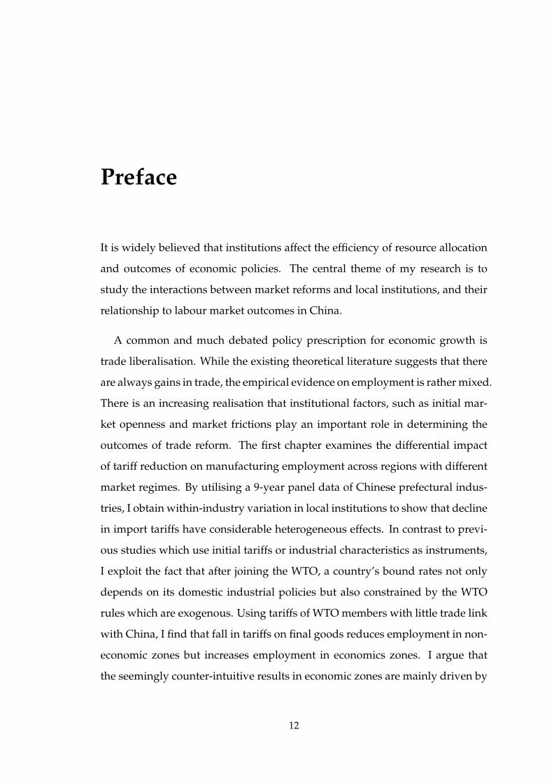
Preface
It is widely believed that institutions affect the efficiency of resource allocation
and outcomes of economic policies. The central theme of my research is to
study the interactions between market reforms and local institutions, and their
relationship to labour market outcomes in China.
A common and much debated policy prescription for economic growth is
trade liberalisation. While the existing theoretical literature suggests that there
are always gains in trade, the empirical evidence on employment is rather mixed.
There is an increasing realisation that institutional factors, such as initial mar-
ket openness and market frictions play an important role in determining the
outcomes of trade reform. The first chapter examines the differential impact
of tariff reduction on manufacturing employment across regions with different
market regimes. By utilising a 9-year panel data of Chinese prefectural indus-
tries, I obtain within-industry variation in local institutions to show that decline
in import tariffs have considerable heterogeneous effects. In contrast to previ-
ous studies which use initial tariffs or industrial characteristics as instruments,
I exploit the fact that after joining the WTO, a country’s bound rates not only
depends on its domestic industrial policies but also constrained by the WTO
rules which are exogenous. Using tariffs of WTO members with little trade link
with China, I find that fall in tariffs on final goods reduces employment in non-
economic zones but increases employment in economics zones. I argue that
the seemingly counter-intuitive results in economic zones are mainly driven by
12
the expansion of foreign enterprises and exporting firms when tariffs were low-
ered. These results highlight the importance of foreign investment and other
pro-trade policies during the process of trade liberalisation.
The presence of regional market segregation not only affects the outcomes
of economic policies but also has potentially large consequences on firms’ be-
haviour and efficiency. The second chapter, which is a collaborative work with
John Morrow and Kitjawat Tacharoen, develops a multi-region, multi-industry
general equilibrium model to explain how regional wage and skill dispersion
affects firm’s location and productivity. The model has two main implications.
First, within sectors, some regions have comparative advantage of lower effec-
tive labour cost than others, and these regions attract more firms per capita.
Second, regional variation in labour costs help explain productivity dispersion
across firms. Based on the model framework, we develop a 2 stage OLS estima-
tion strategy to obtain the effective labour costs which link regional character-
istics to firm’s productivity. Applying our methodology to Chinese manufac-
turing and census data, we find that favourable labour market conditions ex-
plain substantial differences in firm productivity. Regional differences in labour
costs explain 3 to 17 percent of the productivity differences across firm. Also,
labour costs are negatively related to the value-added per capita across regions,
which indicate that firms are more concentrated in regions where labour costs
are lower. This work suggests that increasing labour mobility or reducing factor
price inequality have potentially large gains in the economy.
In additional to market liberalisation, investment in human capital is widely
agreed to be an important element in development process. The last chapter ex-
ploits the exogenous shock to basic education during the Cultural Revolution
to estimate the impact of schooling on occupational status and children’s edu-
cational attainment. Using trend deviations in graduation rates as instruments
of schooling, the results show that education has positive and significant effects
on an individual’s first occupation. Each additional year of schooling increases

the probability of obtaining an off-farm job and white-collar occupation. More-
over, there is a significant causal relationship between parent’s and children’s
education. This suggests that the effects of increased schooling are persistent
across generations.
Chapter 1
Tariffs and Employment: Evidence
from Chinese Manufacturing
Industry
1.1 Introduction
In the past few decades, many developing countries have liberalised their trade
regime with the hope that globalisation would lead to economic growth and
welfare improvement. By removing trade barriers, countries would gain from
cheaper imported inputs and access to export markets, and therefore increase
employment. However, empirical evidence on the employment effects of trade
liberalisation is rather mixed.1 Recent work suggests that domestic institutions
affect the outcomes of market liberalisation (Aghion et al., 2008). Successful
market reforms are often complemented with other supporting policies which
facilitate the reallocation of resource towards more productive uses. On the1For instance, Ghana’s industrial sector was devastated by the increased import competition after
opening its country to foreign trade in 1987. In early 1990s, growth in manufacturing was barely over1% per year and employment in manufacturing fell from 78,700 in 1987 to 28,000 in 1993. Zambia reducedits maximum tariff from 100% to 25% and eliminated most non-tariff barriers between 1992 and 1997.During this period, formal sector employment in manufacturing fell by 40% and manufactures fell as aproportion of GDP.
15
Chapter 1. Tariffs and Employment 16
contrary, market liberalisation can be detrimental to growth with the presence
of unfavourable institutions.
The aim of this paper is to explore the impact of trade liberalisation on re-
gional manufacturing employment and, in particular, how the effects vary across
regions under different market regimes. I focus on China, which reduced im-
port tariffs significantly after its accession to the WTO in December 2001. Be-
tween 1998 and 2006, average tariffs on agricultural and industrial products fell
from 22% to 17.5% and 24.6% to 9.4% respectively. During the same period, im-
port values grew at an average annual rate of 25%, from USD 140 billion in 1998
to USD 791 billion in 2006. I investigate the role of market-oriented policies on
the effects of tariff decline by exploiting the fact that institutions vary consider-
ably across regions in China due to its earlier reform policy. Since 1980, China
has established more than a hundred economic zones of various types through-
out the country.2 Economic zones have more liberalized economies and offer a
number of preferential policies which encourage foreign investment and export
activities. With greater autonomy and integration with international markets,
industries in economic zones lead the country in technology and productivity
growth.
Tariff protection is endogenous as it is correlated with unobservable time-
varying industrial characteristics which affect tariffs and employment simulta-
neously (Trefler 1994; 2004). I am particularly concerned about the endogeneity
of tariff reduction after China’s WTO accession since China’s bound rates were
negotiated between China and other WTO members, and special exemptions
were granted to certain industries.3 I depart from the previous studies which
use pre-reform tariff levels and industry characteristics as instruments for fu-
ture tariff changes (Trefler 1993; 2004; Goldberg and Pavcnik 2005; Amiti and2In China, economic zones include special economic zones, coastal open cities, coastal economic zones,
national and provincial economic and technological development zones, export-processing zones, high-tech zones and industrial parks. Many economic zones locate in same prefectures.
3Bound rates are maximum tariff rates allowed by the WTO to charge on imports from other WTOmember states. They are negotiated between the new member and other WTO states before accession.
Chapter 1. Tariffs and Employment 17
Konings 2007; Amiti and Davis 2012). Instead, I adopt an instrumental vari-
able strategy which takes advantage of the fact that after joining the WTO, a
country’s bound rates not only depends on its domestic industrial policies but
also constrained by the WTO rules on tariffs which are exogenous. I show that
tariffs of other WTO members are strong instruments for China’s post-WTO tar-
iffs if two conditions are satisfied. First, China and other members’ tariffs are
bound by common WTO rules. Second, they have different industrial charac-
teristics from China. Countries which joined the WTO between 2000 and 2003
have similar average bound rates but different economic structure and limited
trade links with China. Therefore, I construct the instruments for China’s tar-
iffs by combining the bound rates of these countries.4 The main advantage of
my instrumental variable strategy over the conventional approaches is the ex-
ogeneity assumption still holds even if there is serial correlation in industry
characteristics.
Using the Annual Surveys of Industrial Firms, I construct an unbalanced
panel of prefecture-industries spanning the period from 1998 to 2006. The re-
gional industry data includes 109 4-digit ISIC industries across 336 prefectures,
among which 49 have established at least one economic zone before 2000. The
data is then matched with 4-digit industry tariffs. The impact of tariff reduction
is decomposed into two effects: reduction in output tariff (tariffs on imported
final goods) and reduction in input tariffs (tariffs on imported intermediate in-
puts) (Amiti and Konings, 2007). A fall in output tariffs increases the degree
of import competition while a fall in input tariffs reduces production costs and
increases the variety of intermediate input available.
My IV estimates suggest that tariff reduction has insignificant impact on4Between 2000 and 2003, eleven countries joined the WTO. They include Jordan, Georgia, Albania,
Oman, Croatia, Lithuania, Moldova, China, Taiwan, Armenia and Macedonia.
Chapter 1. Tariffs and Employment 18
employment on average; however, the effects vary considerably across eco-
nomic and non-economic zones.5 A 1% fall in output tariffs increases employ-
ment in economic zones by 0.43% but reduces employment in non-economic
zones by 0.57%. Similarly, a 1% fall in input tariffs reduces employment in
economic zones by 0.93% but increases employment in non-economic zones by
0.75%. This suggests that tariff reduction has strong reallocation effects. Em-
ployment adjustments in economic zones are mainly driven by the expansion
of foreign and exporting firms in industries which faced larger output tariff
cuts but smaller input tariff changes. By restricting the sample to coastal eco-
nomic zones and their nearby prefectures, I show that my results are not entirely
driven by the geographical factors. Yet, the results do suggest that among non-
economic zones, the impact of tariff reduction is larger in inland prefectures
which have less favourable regulatory and economic conditions compared to
its eastern counterparts. Our estimates are robust to controlling non-tariff bar-
riers and changes in tariffs on Chinese exports.
This study is relevant to the recent empirical literature on the heterogeneous
effects of market liberalisation. Amiti and Konings (2007) find that reductions
in output and input tariffs increase firm’s productivity and the size of effects
vary with firm’s export and import orientation. Another paper by Amiti and
Davis (2012) studies the relationship between tariffs and firm wages suggests
that firm’s initial trade status could explain the heterogeneous effects of tariff
reduction on firm’s wages. Aghion et al. (2008) analyse how the delicensing of
manufacturing industry interacts with local labour market regulations in India.
They find that the delicensing reform increased industrial output of states with
pro-employer regulations but reduced output of states with pro-labour regula-
tions.
The rest of the paper is organised as follows. In Section 2, I describe the5Since my unit of analysis is a prefecture-industry, I identify prefectures which have established eco-
nomic zones and use the terms ‘economic zones’ and ‘prefectures with economic zones’ interchangeablyin this paper.
Chapter 1. Tariffs and Employment 19
background of the two reforms which are relevant to this study. Section 3 ex-
plains my empirical strategy and Section 4 describes the data. In Section 5, I
discuss the mechanism and in Section 6, I present the empirical results. Section
7 interprets the results and Section 8 concludes.
1.2 Background
1.2.1 Tariffs and WTO Accession
When China joined the WTO in December 2001, it committed to reduce tariffs
significantly within five years of accession.6 60% of the products’ tariffs were
reduced below their final bound tariff rates within 1 year of accession; and by
2005, 98% of the products’ tariffs were bound.7 The degree of trade liberali-
sation varied significantly across industries. To satisfy the WTO general rules
on tariffs, industries with higher tariff protection were required to make larger
concessions. Since China is a developing country, exemptions were granted for
certain key products.
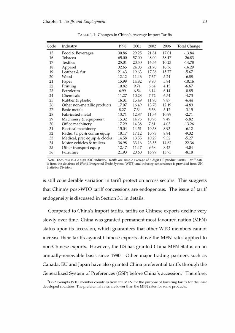
Table 1.1 reports the changes in China’s average import tariffs for 2-digit ISIC
manufacturing industry.8 It shows that China’s pre-WTO tariffs were higher for
industries with large state interests, such as tobacco, beverages and motor vehi-
cles (more than 30%), and lower for raw materials which are abundant in China,
such as petroleum, chemicals and basic materials (less than 15%). Major tariff
cuts occurred in 2002 where industries with higher pre-WTO tariffs experienced
larger fall in tariffs. Between 1998 and 2006, average tariffs on tobacco products
and motor vehicles fell by more than 20% while tariffs on petroleum and basic
materials reduced by 1 to 3% only. Although tariffs converge over time, there6China is required to reduce tariffs across ten years but major tariff cuts occured between 2002 and
2005.7Figures are based on author’s calculations using 8-digit HS tariff data from WITS and China’s Sched-
ule of Concessions.8Industry tariffs is the simple average of 8-digit HS product tariffs. Concordance table for HS and ISIC
Rev. 3 codes is obtained from UNSTAT.
Chapter 1. Tariffs and Employment 20
TABLE 1.1: Changes in China’s Average Import Tariffs
Code Industry 1998 2001 2002 2006 Total Change
15 Food & Beverages 30.86 29.25 21.81 17.01 -13.8416 Tobacco 65.00 57.00 48.00 38.17 -26.8317 Textiles 25.01 20.50 16.56 10.23 -14.7818 Apparel 32.65 24.03 21.70 16.36 -16.2919 Leather & fur 21.43 19.63 17.38 15.77 -5.6720 Wood 12.12 11.46 7.37 5.24 -6.8821 Paper 15.99 14.82 9.90 5.84 -10.1622 Printing 10.82 9.71 6.64 4.15 -6.6723 Petroleum 6.99 6.54 6.14 6.14 -0.8524 Chemicals 11.27 10.28 7.72 6.54 -4.7325 Rubber & plastic 16.31 15.49 11.90 9.87 -6.4426 Other non-metallic products 17.07 16.49 13.78 12.19 -4.8927 Basic metals 8.27 7.34 5.56 5.12 -3.1528 Fabricated metal 13.71 12.87 11.36 10.99 -2.7129 Machinery & equipment 15.32 14.75 10.96 9.49 -5.8230 Office machinery 17.29 14.38 7.81 4.03 -13.2631 Electical machinery 15.04 14.51 10.38 8.93 -6.1232 Radio, tv, pc & comm equip 18.17 17.12 10.73 8.84 -9.3233 Medical, prec equip & clocks 14.58 13.55 10.29 9.32 -5.2734 Motor vehicles & trailers 36.98 33.16 23.55 14.62 -22.3635 Other transport equip 12.47 11.47 9.68 8.43 -4.0436 Furniture 21.93 20.60 16.99 13.75 -8.18
Note: Each row is a 2-digit ISIC industry. Tariffs are simple average of 8-digit HS product tariffs. Tariff datais from the database of World Integrated Trade System (WITS) and industry concordance is provided from UNStatistics Division.
is still considerable variation in tariff protection across sectors. This suggests
that China’s post-WTO tariff concessions are endogenous. The issue of tariff
endogeneity is discussed in Section 3.1 in details.
Compared to China’s import tariffs, tariffs on Chinese exports decline very
slowly over time. China was granted permanent most-favoured nation (MFN)
status upon its accession, which guarantees that other WTO members cannot
increase their tariffs against Chinese exports above the MFN rates applied to
non-Chinese exports. However, the US has granted China MFN Status on an
annually-renewable basis since 1980. Other major trading partners such as
Canada, EU and Japan have also granted China preferential tariffs through the
Generalized System of Preferences (GSP) before China’s accession.9 Therefore,9GSP exempts WTO member countries from the MFN for the purpose of lowering tariffs for the least
developed countries. The preferential rates are lower than the MFN rates for some products.
Chapter 1. Tariffs and Employment 21
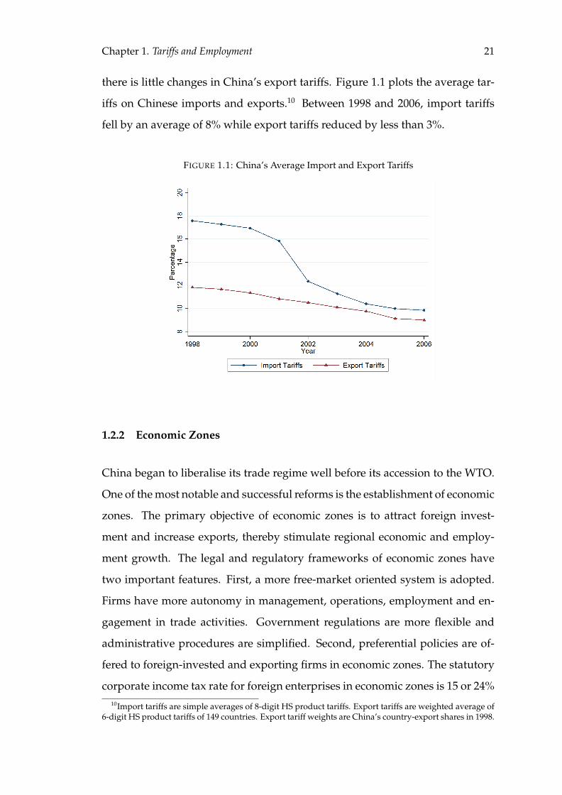
there is little changes in China’s export tariffs. Figure 1.1 plots the average tar-
iffs on Chinese imports and exports.10 Between 1998 and 2006, import tariffs
fell by an average of 8% while export tariffs reduced by less than 3%.
FIGURE 1.1: China’s Average Import and Export Tariffs
1.2.2 Economic Zones
China began to liberalise its trade regime well before its accession to the WTO.
One of the most notable and successful reforms is the establishment of economic
zones. The primary objective of economic zones is to attract foreign invest-
ment and increase exports, thereby stimulate regional economic and employ-
ment growth. The legal and regulatory frameworks of economic zones have
two important features. First, a more free-market oriented system is adopted.
Firms have more autonomy in management, operations, employment and en-
gagement in trade activities. Government regulations are more flexible and
administrative procedures are simplified. Second, preferential policies are of-
fered to foreign-invested and exporting firms in economic zones. The statutory
corporate income tax rate for foreign enterprises in economic zones is 15 or 24%10Import tariffs are simple averages of 8-digit HS product tariffs. Export tariffs are weighted average of
6-digit HS product tariffs of 149 countries. Export tariff weights are China’s country-export shares in 1998.
Chapter 1. Tariffs and Employment 22
while the national average is 33%.11 Also, tariffs on imported materials and
machinery are exempted for exported products in economic zones.
The earliest economic zones in China can be traced back to 1980 when four
Special Economic Zones were established in Guangdong and Fujian Province.
In 1984, fourteen coastal cities were opened to foreign investment, and in 1988,
the entire Hainan Province was designated as a Special Economic Zone. Be-
tween 1984 and 1994, thirty four National Economic and Technological Devel-
opment Zones and two Coastal Economic Zones were set up in China. Af-
ter 2000, there was a rapid expansion of economic zones in inland China to
take advantage of the increased export opportunities after China’s accession to
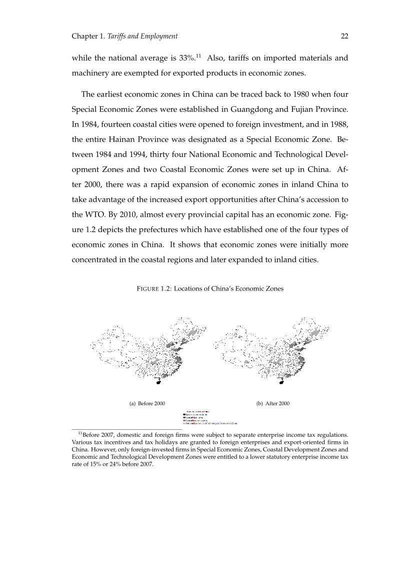
the WTO. By 2010, almost every provincial capital has an economic zone. Fig-
ure 1.2 depicts the prefectures which have established one of the four types of
economic zones in China. It shows that economic zones were initially more
concentrated in the coastal regions and later expanded to inland cities.
FIGURE 1.2: Locations of China’s Economic Zones
(a) Before 2000 (b) After 2000
11Before 2007, domestic and foreign firms were subject to separate enterprise income tax regulations.Various tax incentives and tax holidays are granted to foreign enterprises and export-oriented firms inChina. However, only foreign-invested firms in Special Economic Zones, Coastal Development Zones andEconomic and Technological Development Zones were entitled to a lower statutory enterprise income taxrate of 15% or 24% before 2007.
Chapter 1. Tariffs and Employment 23
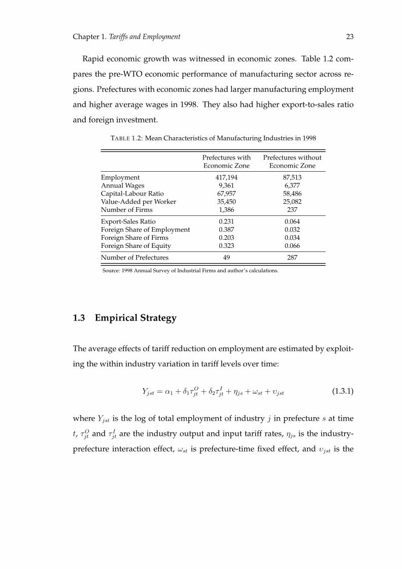
Rapid economic growth was witnessed in economic zones. Table 1.2 com-
pares the pre-WTO economic performance of manufacturing sector across re-
gions. Prefectures with economic zones had larger manufacturing employment
and higher average wages in 1998. They also had higher export-to-sales ratio
and foreign investment.
TABLE 1.2: Mean Characteristics of Manufacturing Industries in 1998
Prefectures with Prefectures withoutEconomic Zone Economic Zone
Employment 417,194 87,513Annual Wages 9,361 6,377Capital-Labour Ratio 67,957 58,486Value-Added per Worker 35,450 25,082Number of Firms 1,386 237
Export-Sales Ratio 0.231 0.064Foreign Share of Employment 0.387 0.032Foreign Share of Firms 0.203 0.034Foreign Share of Equity 0.323 0.066
Number of Prefectures 49 287
Source: 1998 Annual Survey of Industrial Firms and author’s calculations.
1.3 Empirical Strategy
The average effects of tariff reduction on employment are estimated by exploit-
ing the within industry variation in tariff levels over time:
Yjst = α1 + δ1τOjt + δ2τ
Ijt + ηjs + ωst + υjst (1.3.1)
where Yjst is the log of total employment of industry j in prefecture s at time
t, τOjt and τ Ijt are the industry output and input tariff rates, ηjs is the industry-
prefecture interaction effect, ωst is prefecture-time fixed effect, and υjst is the
Chapter 1. Tariffs and Employment 24
stochastic error term12. The industry-prefecture fixed effects capture the vari-
ation in regional industry policies such as local industrial subsidies, and the
prefecture-time fixed effects controls for other time-varying regional character-
istics such improvement in infrastructure, proximity to markets, and migration
trends. Standard errors are clustered by industry and year.
The differential impact of tariff reduction in economic and non-economic
zones is estimated by the following specification:
Yjst = α2 + β1τOjt + β2τ
Ijt + β3τ
Ojt × EZs + β4τ
Ijt × EZs + ηjs + ωst + υjst
where EZs is a dummy which equals to one if prefecture s has created an eco-
nomic zone before 2000. I focus on the four types of economic zones: Special
Economic Zones, Coastal Open Cities, Coastal Economic Zones and National
Economic and Technological Development Zones. Economic zones established
after 2000 are classified as non-economic zones in this analysis since their cre-
ation are likely to be endogenous to China’s tariff reduction. Some of these
economic zones are at prefecture level while others are at more disaggregated
county level. Since my unit of analysis is a prefecture-industry, the estimates
of equation (1.3.2) would provide the lower bound of the true effects of eco-
nomic zones. For simplification, the terms ‘economic zones’ and ‘prefectures
with economic zones’ are used interchangeably in this paper.
In equation (1.3.2), β1 and β2 measure the percentage change in total employ-
ment in non-economic zones when tariffs fall by 1%, while β1 + β3 and β2 + β4
measure the percentage change in employment in economic zones. Therefore,
the relative signs of βs capture the heterogeneous effects of tariff reduction in
economic and non-economic zones. If β1 and β2 have the same signs as β3 and12A number of studies estimate the impact of tariffs in differences instead of levels (Trefler, 2004; Gold-
berg and Pavcnik, 2005; Yu, 2011; Amiti and Davis, 2012). The advantage of estimating in long differencesis it allows firms to have longer time to adjust wages and employment. If there are serial correlations inemployment and wages, taking long differences would generate unbiased estimates. However, estimat-ing in differences is not suitable in this context. In China, tariffs fell at unequal rates across time. Tariffchanges were minimal in 1998 to 2001 and 2002 to 2006, yet tariff levels were much lower in 2002-2006. Ifwe take less than three-year differences, we would wrongly assume that the treatment effects in 1998 to2001 and 2002 to 2006 are the same.
Chapter 1. Tariffs and Employment 25
β4 respectively, then reduction in tariffs have larger effects in economic zones.
If the signs are reversed, then tariff cuts have smaller or opposite effects in eco-
nomic zones.
1.3.1 Tariff Endogeneity
Our OLS estimates for equations (1.3.1) and (1.3.2) would be biased with the
presence of time-varying industry characteristics which are correlated with em-
ployment and tariffs. The endogeneity of trade protection is well documented
in the existing trade literature. Trefler (1993; 1994) argues that trade protection
are determined by two broad factors: the cost of coordinating lobbying and the
interests of politicians. Industries with lower opportunity cost of lobbying and
larger gains from protection would have greater trade protection.
In China, industries are more protected either because they are important sources
of government revenue or crucial to national interest. As shown in Table 1.1 pre-
viously, industry tariffs varied considerably even after China’s accession to the
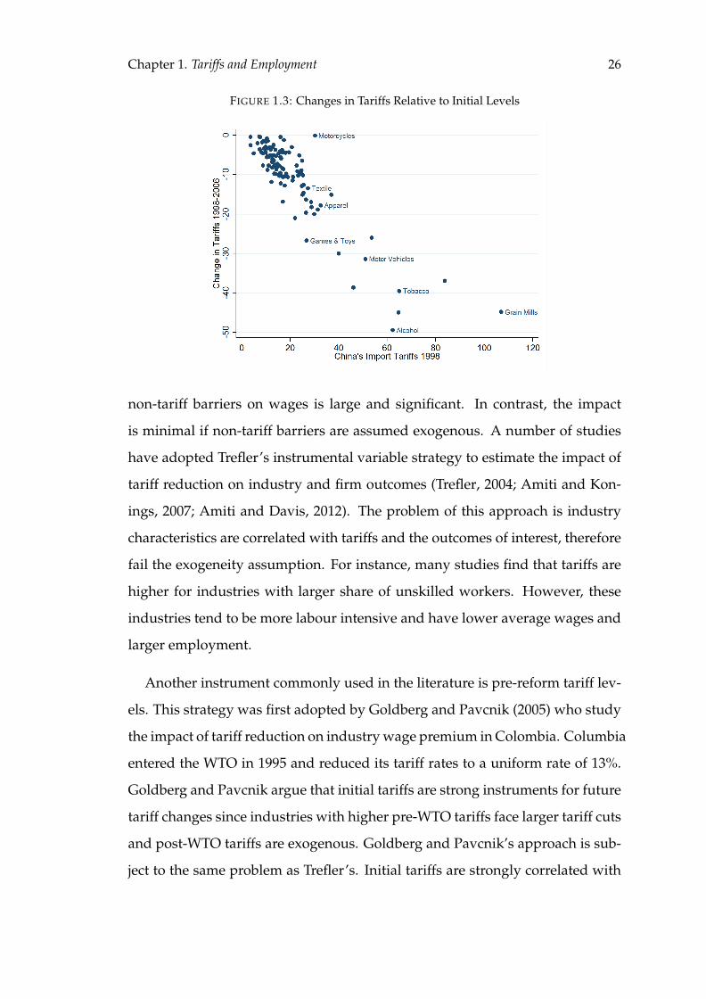
WTO. Figure 1.3 plots the percentage change in China’s import tariffs against
the initial tariff levels for 4-digit ISIC. It shows that the extent of tariff reduction
was unequal across sectors with similar initial tariff levels. For instance, tariffs
on games and toys and motorcycles were about 35% in 1998. However, tariffs
on games and toys fell by 20% in 2006 while tariffs on motorcycles reduced by
only 0.5%.
The direction of bias is uncertain. Fast growing industries might have lower
tariffs because they can compete with foreign competition. Industries might
also experience higher growth rate because they were more protected. The for-
mer would lead to an upward bias of the OLS estimates while the latter would
lead to a downward bias of the OLS estimates.
Since tariffs depend on political and economic factors, Trefler (1993) uses in-
dustry characteristics such as market concentration ratio and degree of import
penetration as instruments for non-tariff barriers and finds that the impact of
Chapter 1. Tariffs and Employment 26
FIGURE 1.3: Changes in Tariffs Relative to Initial Levels
non-tariff barriers on wages is large and significant. In contrast, the impact
is minimal if non-tariff barriers are assumed exogenous. A number of studies
have adopted Trefler’s instrumental variable strategy to estimate the impact of
tariff reduction on industry and firm outcomes (Trefler, 2004; Amiti and Kon-
ings, 2007; Amiti and Davis, 2012). The problem of this approach is industry
characteristics are correlated with tariffs and the outcomes of interest, therefore
fail the exogeneity assumption. For instance, many studies find that tariffs are
higher for industries with larger share of unskilled workers. However, these
industries tend to be more labour intensive and have lower average wages and
larger employment.
Another instrument commonly used in the literature is pre-reform tariff lev-
els. This strategy was first adopted by Goldberg and Pavcnik (2005) who study
the impact of tariff reduction on industry wage premium in Colombia. Columbia
entered the WTO in 1995 and reduced its tariff rates to a uniform rate of 13%.
Goldberg and Pavcnik argue that initial tariffs are strong instruments for future
tariff changes since industries with higher pre-WTO tariffs face larger tariff cuts
and post-WTO tariffs are exogenous. Goldberg and Pavcnik’s approach is sub-
ject to the same problem as Trefler’s. Initial tariffs are strongly correlated with
Chapter 1. Tariffs and Employment 27
industry characteristics, and therefore are endogenous.13
1.3.2 Instrumental Variable Strategy
I adopt a new approach to tackle the problem of tariff endogeneity. According
to the WTO principles of trading system, tariffs should be reduced and bound
against future increase. Tariff commitments made by countries are reached
through multilateral negotiations among WTO member states. Each country
is obliged not to increase tariffs above the bound rates listed in its schedule of
concessions. Special exemptions and longer transition period are granted to
developing countries taking into account their level of economic development
and specific trade needs. Since the terms of accession are unique for each coun-
try, I find considerable cross-country variation in bound rates within industries.
For example, the average bound rate for motorcycles is 30% in China but only
9% and 13.4% in Macedonia and Croatia respectively. Since bound rates tend to
be higher for industries with larger state interests, tariffs of countries which are
required to make larger tariff concessions would better reflect the WTO general
rules on tariffs.
By 2010, the WTO has 157 member states, so the question is which country’s
tariffs are suitable instruments for China’s tariffs. Our choice of instruments is
guided by a simple econometric model. Suppose a country’s tariff policy can
be summarized by the following specification:
τjkt = αk + π′kθjkt + δ′k(Dkt ∗WTOjkt) + ujkt (1.3.2)
where τjkt is the tariff rate of industry j in country k at time t, θjkt captures the
industry-time effect, Dkt is a dummy which equals to 1 if country k is a member
of the WTO, and WTOjkt is the WTO rule on the country k’s industry tariffs.13Suppose θjt are unobservable time-varying political-economic factors that are correlated with tariffs
and I use intital tariffs τj0 as instruments for future tariff changes. Then τj0 is a good instrument if therelevance and exogeneity assumptions are satisfied i.e. Cov(τj0,∆τjt) 6= 0 and Cov(τj0,∆θjt) = 0. It canbe immediately shown that two conditions cannot be satisfied simultaneously if τjt = f(θjt).
Chapter 1. Tariffs and Employment 28
Equation (1.3.2) suggests that a country’s bound rates depends on its industry
characteristics and the WTO rules after its accession. Our identification strategy
requires the following two conditions to be satisfied:
Cov(τkjt, τjt) 6= 0 (1.3.3)
Cov(τkjt, θjt) = 0 (1.3.4)
where τjt and θjt are the industry tariffs and time-varying industry characteris-
tics of China respectively. Substituting equation (1.3.2) into the equations (1.3.3)
and (1.3.4) suggest that
Cov(WTOjt,WTOkjt) 6= 0 (1.3.5)
Cov(θjt, θkjt) = 0 (1.3.6)
Condition (1.3.5) requires China and country k to be subject to common ex-
ogenous WTO rules while condition (1.3.6) suggests that country k’s industry
should not affect China’s employment via its impact on China’s industry devel-
opment.
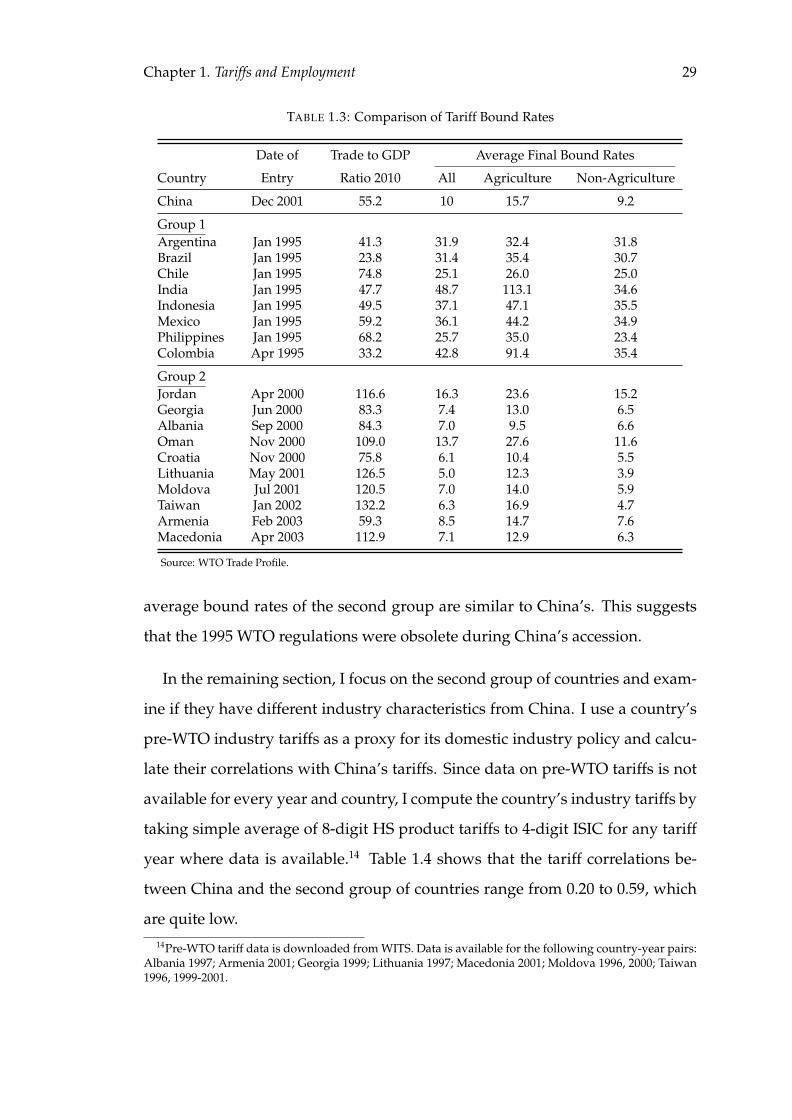
Table 1.3 compares the China and other WTO members’ final bound rates.
Countries are divided into two groups based on their comparability with China
and date of WTO accession. The first group consists of large developing coun-
tries and Southeast Asian countries such as Brazil, India and the Philippines.
By coincidence, all of them joined the WTO in 1995. The second group in-
cludes all countries which joined the WTO between 2000 and 2003. The average
bound rates of new WTO members decline with their year of accession as the
WTO regulations become more stringent over time. Hence, although the first
group of countries are more comparable to China in terms of economic size or
level of economic development, their average bound rates are much higher than
China’s as they joined the WTO earlier than China (above 25%). In contrast, the
Chapter 1. Tariffs and Employment 29
TABLE 1.3: Comparison of Tariff Bound Rates
Date of Trade to GDP Average Final Bound Rates
Country Entry Ratio 2010 All Agriculture Non-Agriculture
China Dec 2001 55.2 10 15.7 9.2
Group 1Argentina Jan 1995 41.3 31.9 32.4 31.8Brazil Jan 1995 23.8 31.4 35.4 30.7Chile Jan 1995 74.8 25.1 26.0 25.0India Jan 1995 47.7 48.7 113.1 34.6Indonesia Jan 1995 49.5 37.1 47.1 35.5Mexico Jan 1995 59.2 36.1 44.2 34.9Philippines Jan 1995 68.2 25.7 35.0 23.4Colombia Apr 1995 33.2 42.8 91.4 35.4
Group 2Jordan Apr 2000 116.6 16.3 23.6 15.2Georgia Jun 2000 83.3 7.4 13.0 6.5Albania Sep 2000 84.3 7.0 9.5 6.6Oman Nov 2000 109.0 13.7 27.6 11.6Croatia Nov 2000 75.8 6.1 10.4 5.5Lithuania May 2001 126.5 5.0 12.3 3.9Moldova Jul 2001 120.5 7.0 14.0 5.9Taiwan Jan 2002 132.2 6.3 16.9 4.7Armenia Feb 2003 59.3 8.5 14.7 7.6Macedonia Apr 2003 112.9 7.1 12.9 6.3
Source: WTO Trade Profile.
average bound rates of the second group are similar to China’s. This suggests
that the 1995 WTO regulations were obsolete during China’s accession.
In the remaining section, I focus on the second group of countries and exam-
ine if they have different industry characteristics from China. I use a country’s
pre-WTO industry tariffs as a proxy for its domestic industry policy and calcu-
late their correlations with China’s tariffs. Since data on pre-WTO tariffs is not
available for every year and country, I compute the country’s industry tariffs by
taking simple average of 8-digit HS product tariffs to 4-digit ISIC for any tariff
year where data is available.14 Table 1.4 shows that the tariff correlations be-
tween China and the second group of countries range from 0.20 to 0.59, which
are quite low.14Pre-WTO tariff data is downloaded from WITS. Data is available for the following country-year pairs:
Albania 1997; Armenia 2001; Georgia 1999; Lithuania 1997; Macedonia 2001; Moldova 1996, 2000; Taiwan1996, 1999-2001.
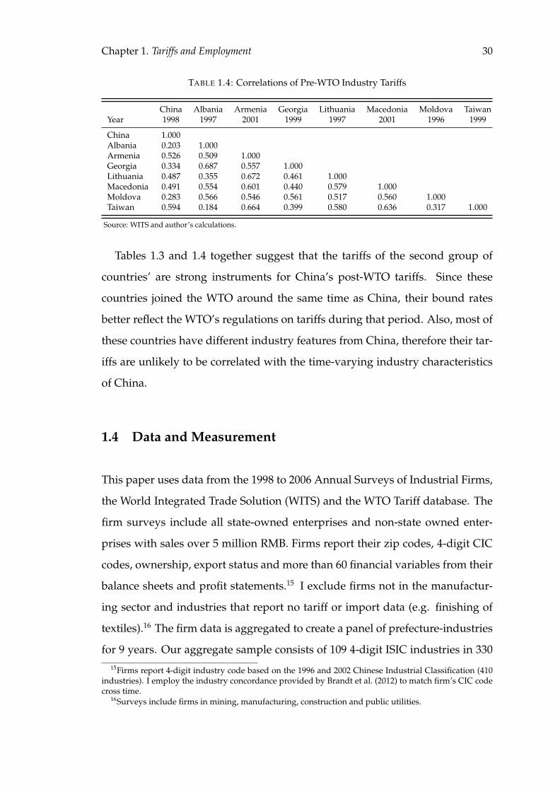
Chapter 1. Tariffs and Employment 30
TABLE 1.4: Correlations of Pre-WTO Industry Tariffs
China Albania Armenia Georgia Lithuania Macedonia Moldova TaiwanYear 1998 1997 2001 1999 1997 2001 1996 1999
China 1.000Albania 0.203 1.000Armenia 0.526 0.509 1.000Georgia 0.334 0.687 0.557 1.000Lithuania 0.487 0.355 0.672 0.461 1.000Macedonia 0.491 0.554 0.601 0.440 0.579 1.000Moldova 0.283 0.566 0.546 0.561 0.517 0.560 1.000Taiwan 0.594 0.184 0.664 0.399 0.580 0.636 0.317 1.000
Source: WITS and author’s calculations.
Tables 1.3 and 1.4 together suggest that the tariffs of the second group of
countries’ are strong instruments for China’s post-WTO tariffs. Since these
countries joined the WTO around the same time as China, their bound rates
better reflect the WTO’s regulations on tariffs during that period. Also, most of
these countries have different industry features from China, therefore their tar-
iffs are unlikely to be correlated with the time-varying industry characteristics
of China.
1.4 Data and Measurement
This paper uses data from the 1998 to 2006 Annual Surveys of Industrial Firms,
the World Integrated Trade Solution (WITS) and the WTO Tariff database. The
firm surveys include all state-owned enterprises and non-state owned enter-
prises with sales over 5 million RMB. Firms report their zip codes, 4-digit CIC
codes, ownership, export status and more than 60 financial variables from their
balance sheets and profit statements.15 I exclude firms not in the manufactur-
ing sector and industries that report no tariff or import data (e.g. finishing of
textiles).16 The firm data is aggregated to create a panel of prefecture-industries
for 9 years. Our aggregate sample consists of 109 4-digit ISIC industries in 33015Firms report 4-digit industry code based on the 1996 and 2002 Chinese Industrial Classification (410
industries). I employ the industry concordance provided by Brandt et al. (2012) to match firm’s CIC codecross time.
16Surveys include firms in mining, manufacturing, construction and public utilities.
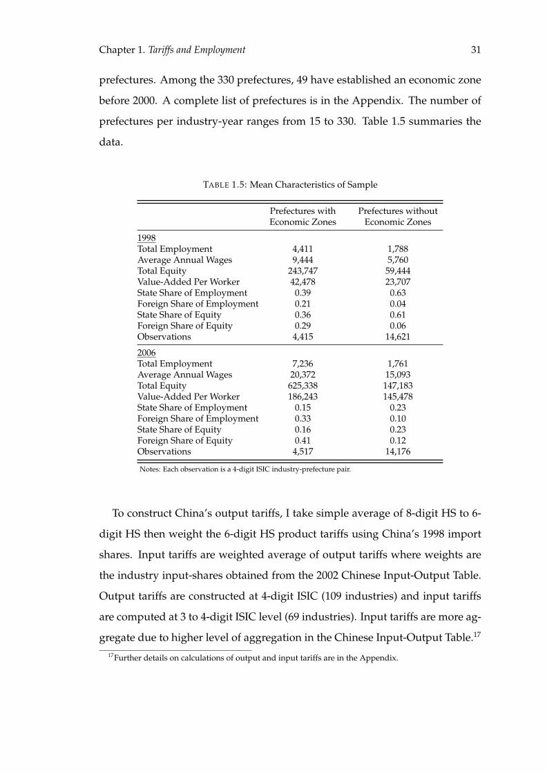
Chapter 1. Tariffs and Employment 31
prefectures. Among the 330 prefectures, 49 have established an economic zone
before 2000. A complete list of prefectures is in the Appendix. The number of
prefectures per industry-year ranges from 15 to 330. Table 1.5 summaries the
data.
TABLE 1.5: Mean Characteristics of Sample
Prefectures with Prefectures withoutEconomic Zones Economic Zones
1998Total Employment 4,411 1,788Average Annual Wages 9,444 5,760Total Equity 243,747 59,444Value-Added Per Worker 42,478 23,707State Share of Employment 0.39 0.63Foreign Share of Employment 0.21 0.04State Share of Equity 0.36 0.61Foreign Share of Equity 0.29 0.06Observations 4,415 14,621
2006Total Employment 7,236 1,761Average Annual Wages 20,372 15,093Total Equity 625,338 147,183Value-Added Per Worker 186,243 145,478State Share of Employment 0.15 0.23Foreign Share of Employment 0.33 0.10State Share of Equity 0.16 0.23Foreign Share of Equity 0.41 0.12Observations 4,517 14,176
Notes: Each observation is a 4-digit ISIC industry-prefecture pair.
To construct China’s output tariffs, I take simple average of 8-digit HS to 6-
digit HS then weight the 6-digit HS product tariffs using China’s 1998 import
shares. Input tariffs are weighted average of output tariffs where weights are
the industry input-shares obtained from the 2002 Chinese Input-Output Table.
Output tariffs are constructed at 4-digit ISIC (109 industries) and input tariffs
are computed at 3 to 4-digit ISIC level (69 industries). Input tariffs are more ag-
gregate due to higher level of aggregation in the Chinese Input-Output Table.17
17Further details on calculations of output and input tariffs are in the Appendix.
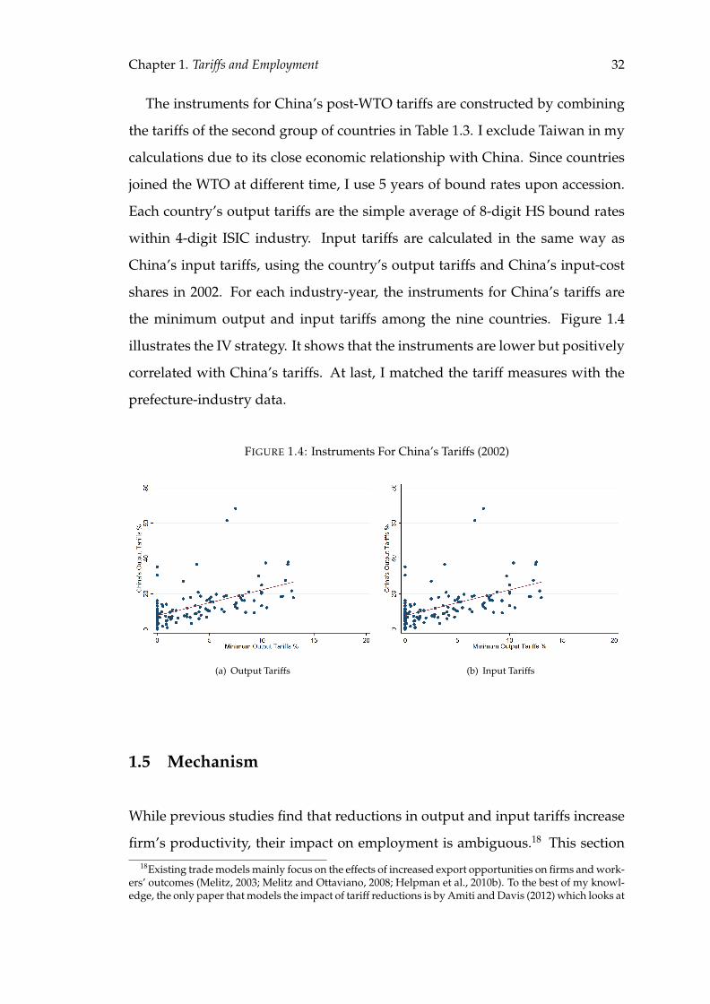
Chapter 1. Tariffs and Employment 32
The instruments for China’s post-WTO tariffs are constructed by combining
the tariffs of the second group of countries in Table 1.3. I exclude Taiwan in my
calculations due to its close economic relationship with China. Since countries
joined the WTO at different time, I use 5 years of bound rates upon accession.
Each country’s output tariffs are the simple average of 8-digit HS bound rates
within 4-digit ISIC industry. Input tariffs are calculated in the same way as
China’s input tariffs, using the country’s output tariffs and China’s input-cost
shares in 2002. For each industry-year, the instruments for China’s tariffs are
the minimum output and input tariffs among the nine countries. Figure 1.4
illustrates the IV strategy. It shows that the instruments are lower but positively
correlated with China’s tariffs. At last, I matched the tariff measures with the
prefecture-industry data.
FIGURE 1.4: Instruments For China’s Tariffs (2002)
(a) Output Tariffs (b) Input Tariffs
1.5 Mechanism
While previous studies find that reductions in output and input tariffs increase
firm’s productivity, their impact on employment is ambiguous.18 This section18Existing trade models mainly focus on the effects of increased export opportunities on firms and work-
ers’ outcomes (Melitz, 2003; Melitz and Ottaviano, 2008; Helpman et al., 2010b). To the best of my knowl-edge, the only paper that models the impact of tariff reductions is by Amiti and Davis (2012) which looks at
Chapter 1. Tariffs and Employment 33
discusses the possible mechanisms that explain the employment outcomes of
tariff concessions.
1.5.1 Direction of Adjustment
Changes in tariff affect the direction of employment adjustment via two chan-
nels. The first one is firm’s profits. Decline in output tariffs reduces the price
of imported final goods, hence increases exposure to foreign competition and
reduces firms’ domestic market share. As firms’ profits are lower, their de-
mand for labour decreases. Aggregate industrial employment decreases in the
intensive and extensive margins, as surviving firms reduce employment and
loss-making firms exit the market.
A fall in input tariffs has opposite effects on firms’ profits. Lower input tariffs
reduce the price of imported inputs, therefore reduce firms’ cost of production
and increases firms’ profits. Aggregate employment increases since existing
firms increase their demand of labour and higher industry profits encourage
new firm entry.
The second channel is related to firms’ product scope and production tech-
nology. Previous studies suggest that access to export markets or external shocks
induce firms to change their product variety (Bernard et al., 2010; Ma et al., 2012;
Bilbiie et al., 2012). Industries subject to larger output tariff cuts face tougher
import competition. Since China has comparative advantage of low labour cost,
firms may produce more labour intensive goods and increase their demand for
labour. Some may choose to produce more capital-intensive or high quality
products that require less unskilled labour to increase their competitiveness and
reduce their demand for labour.the relationship between output and input tariffs and firm wages. Empirical work by Amiti and Konings(2007) and Yu (2011) find that reduction in output and input tariffs increase firm’s productivity; Trefler(2004) shows that reduction in import tariffs reduce manufacturing employment.
Chapter 1. Tariffs and Employment 34
Decline in input tariffs increases the variety and quality of inputs available to
firms, hence allow firms to expand their product scope (Goldberg et al., 2010).
Yet, the effects on employment also depend on the degree of complementarity
between labour and intermediate inputs. If firms increase the share of inter-
mediate inputs in production, and labour and intermediate inputs are comple-
ments, labour demand would increase. In contrast, if the two factor inputs
are substitutes, labour demand and employment would decrease. Therefore,
the net effect on aggregate employment depends on the relative magnitude of
these opposing effects.
1.5.2 Heterogeneous Effects
The effects of tariff reduction are likely to vary across regions for two reasons.
First, local institutions affect the extent of resource reallocation, hence the out-
comes of trade reform. Economic zones have relatively free economy than the
rest of the country, therefore would respond to tariff reduction differently. Re-
gions with stronger local protectionism may impose other trade barriers to off-
set the undesirable effects of import competition. Labour markets rigidities
such as trade unions or unemployment benefits increase the cost of employ-
ment adjustment, thus affect the process of labour reallocation. Credit market
imperfections reduce firms’ ability to offset negative shocks through lending
and borrowing, hence amplify the effects of tariff reduction. Since the reform
outcomes depend on the nature and degree of market frictions, the estimates
capture the joint effects of various institutions and policies on employment.
Apart from market frictions, local institutions and policy measures also affect
the regional composition of firms and therefore the size of adjustment. To take
advantage of the business-friendly environment and preferential policies, for-
eign enterprises and exporting firms are more concentrated in economic zones.
Compared with domestic non-exporting firms, foreign enterprises and export-
ing firms are more productive and larger in size on average. Also, the product
Chapter 1. Tariffs and Employment 35
scope and technological level vary across firm types within a sector. Therefore,
employment adjustment would differ across regions.
Third, some regions have more advantageous geographical position than
others. As shown in Figure 1.2 previously, economic zones established before
2000 are mainly located along the coastal regions which have close proximity
to foreign markets and port terminals. With larger market size and lower trans-
port cost, industries in economic zones may have higher profit margins than
those in inland prefectures which allow them to maintain more internal capital
to smooth employment.
1.6 Empirical Results
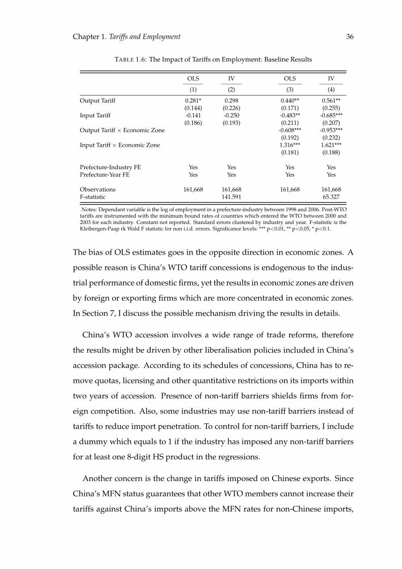
Table 1.6 displays the estimation results for equations (1.3.1) and (1.3.2). The
OLS estimates in column 1 suggest that a 1% fall in output tariffs reduces pre-
fectural employment by an average of 0.28%. A 1% drop in input tariffs in-
creases employment by 0.14% on average but the estimate is insignificant. In
column 2, I instrument China’s post-WTO tariffs with the bound rates of other
countries. The F-statistics reported in the last line of the table are well above
10. The IV estimates are similar to the OLS estimates but very imprecise, which
suggest that tariff reduction has insignificant impact on employment.
Columns 3 and 4 show that there are considerable regional heterogeneity in
the effects of tariff cuts. The OLS results imply that tariff cuts have opposite
impact in economic zone and non-economic zones. A fall in output tariffs re-
duces employment in non-economic zones (0.44) and increases employment in
economic zones (-0.17). Similarly, a fall in input tariffs increases employment in
non-economic zones (-0.48) and reduces employment in economic zones (0.83).
The IV estimates suggest larger heterogeneous effects than the OLS esti-
mates. This implies that output tariffs of fast-growing industries and input
tariffs of slow-growth industries fell to a greater extent in non-economic zones.
Chapter 1. Tariffs and Employment 36
TABLE 1.6: The Impact of Tariffs on Employment: Baseline Results
OLS IV OLS IV
(1) (2) (3) (4)
Output Tariff 0.281* 0.298 0.440** 0.561**(0.144) (0.226) (0.171) (0.255)
Input Tariff -0.141 -0.250 -0.483** -0.685***(0.186) (0.193) (0.211) (0.207)
Output Tariff × Economic Zone -0.608*** -0.953***(0.192) (0.232)
Input Tariff × Economic Zone 1.316*** 1.621***(0.181) (0.188)
Prefecture-Industry FE Yes Yes Yes YesPrefecture-Year FE Yes Yes Yes Yes
Observations 161,668 161,668 161,668 161,668F-statistic 141.591 65.327
Notes: Dependant variable is the log of employment in a prefecture-industry between 1998 and 2006. Post-WTOtariffs are instrumented with the minimum bound rates of countries which entered the WTO between 2000 and2003 for each industry. Constant not reported. Standard errors clustered by industry and year. F-statistic is theKleibergen-Paap rk Wald F statistic for non i.i.d. errors. Significance levels: *** p<0.01, ** p<0.05, * p<0.1.
The bias of OLS estimates goes in the opposite direction in economic zones. A
possible reason is China’s WTO tariff concessions is endogenous to the indus-
trial performance of domestic firms, yet the results in economic zones are driven
by foreign or exporting firms which are more concentrated in economic zones.
In Section 7, I discuss the possible mechanism driving the results in details.
China’s WTO accession involves a wide range of trade reforms, therefore
the results might be driven by other liberalisation policies included in China’s
accession package. According to its schedules of concessions, China has to re-
move quotas, licensing and other quantitative restrictions on its imports within
two years of accession. Presence of non-tariff barriers shields firms from for-
eign competition. Also, some industries may use non-tariff barriers instead of
tariffs to reduce import penetration. To control for non-tariff barriers, I include
a dummy which equals to 1 if the industry has imposed any non-tariff barriers
for at least one 8-digit HS product in the regressions.
Another concern is the change in tariffs imposed on Chinese exports. Since
China’s MFN status guarantees that other WTO members cannot increase their
tariffs against China’s imports above the MFN rates for non-Chinese imports,
Chapter 1. Tariffs and Employment 37
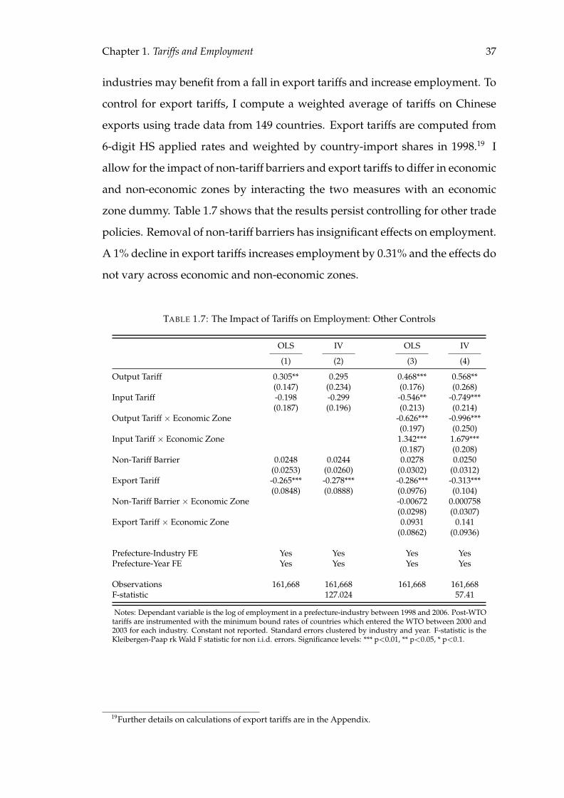
industries may benefit from a fall in export tariffs and increase employment. To
control for export tariffs, I compute a weighted average of tariffs on Chinese
exports using trade data from 149 countries. Export tariffs are computed from
6-digit HS applied rates and weighted by country-import shares in 1998.19 I
allow for the impact of non-tariff barriers and export tariffs to differ in economic
and non-economic zones by interacting the two measures with an economic
zone dummy. Table 1.7 shows that the results persist controlling for other trade
policies. Removal of non-tariff barriers has insignificant effects on employment.
A 1% decline in export tariffs increases employment by 0.31% and the effects do
not vary across economic and non-economic zones.
TABLE 1.7: The Impact of Tariffs on Employment: Other Controls
OLS IV OLS IV
(1) (2) (3) (4)
Output Tariff 0.305** 0.295 0.468*** 0.568**(0.147) (0.234) (0.176) (0.268)
Input Tariff -0.198 -0.299 -0.546** -0.749***(0.187) (0.196) (0.213) (0.214)
Output Tariff × Economic Zone -0.626*** -0.996***(0.197) (0.250)
Input Tariff × Economic Zone 1.342*** 1.679***(0.187) (0.208)
Non-Tariff Barrier 0.0248 0.0244 0.0278 0.0250(0.0253) (0.0260) (0.0302) (0.0312)
Export Tariff -0.265*** -0.278*** -0.286*** -0.313***(0.0848) (0.0888) (0.0976) (0.104)
Non-Tariff Barrier × Economic Zone -0.00672 0.000758(0.0298) (0.0307)
Export Tariff × Economic Zone 0.0931 0.141(0.0862) (0.0936)
Prefecture-Industry FE Yes Yes Yes YesPrefecture-Year FE Yes Yes Yes Yes
Observations 161,668 161,668 161,668 161,668F-statistic 127.024 57.41
Notes: Dependant variable is the log of employment in a prefecture-industry between 1998 and 2006. Post-WTOtariffs are instrumented with the minimum bound rates of countries which entered the WTO between 2000 and2003 for each industry. Constant not reported. Standard errors clustered by industry and year. F-statistic is theKleibergen-Paap rk Wald F statistic for non i.i.d. errors. Significance levels: *** p<0.01, ** p<0.05, * p<0.1.
19Further details on calculations of export tariffs are in the Appendix.
Chapter 1. Tariffs and Employment 38
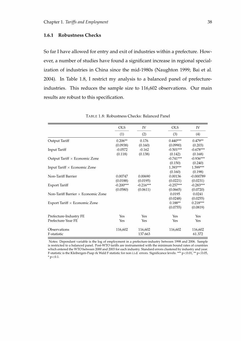
1.6.1 Robustness Checks
So far I have allowed for entry and exit of industries within a prefecture. How-
ever, a number of studies have found a significant increase in regional special-
ization of industries in China since the mid-1980s (Naughton 1999; Bai et al.
2004). In Table 1.8, I restrict my analysis to a balanced panel of prefecture-
industries. This reduces the sample size to 116,602 observations. Our main
results are robust to this specification.
TABLE 1.8: Robustness Checks: Balanced Panel
OLS IV OLS IV
(1) (2) (3) (4)
Output Tariff 0.206** 0.176 0.440*** 0.479**(0.0938) (0.160) (0.0990) (0.203)
Input Tariff -0.0572 -0.162 -0.501*** -0.678***(0.118) (0.138) (0.142) (0.168)
Output Tariff × Economic Zone -0.741*** -0.936***(0.150) (0.240)
Input Tariff × Economic Zone 1.393*** 1.599***(0.160) (0.198)
Non-Tariff Barrier 0.00747 0.00690 0.00136 -0.000789(0.0188) (0.0195) (0.0221) (0.0231)
Export Tariff -0.200*** -0.216*** -0.257*** -0.283***(0.0580) (0.0611) (0.0665) (0.0720)
Non-Tariff Barrier × Economic Zone 0.0195 0.0241(0.0248) (0.0255)
Export Tariff × Economic Zone 0.188** 0.218***(0.0755) (0.0819)
Prefecture-Industry FE Yes Yes Yes YesPrefecture-Year FE Yes Yes Yes Yes
Observations 116,602 116,602 116,602 116,602F-statistic 137.663 61.372
Notes: Dependant variable is the log of employment in a prefecture-industry between 1998 and 2006. Sampleis restricted to a balanced panel. Post-WTO tariffs are instrumented with the minimum bound rates of countrieswhich entered the WTO between 2000 and 2003 for each industry. Standard errors clustered by industry and year.F-statistic is the Kleibergen-Paap rk Wald F statistic for non i.i.d. errors. Significance levels: *** p<0.01, ** p<0.05,* p<0.1.
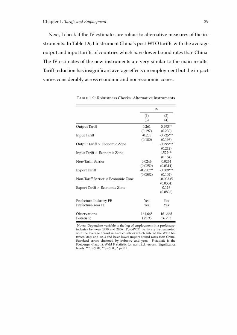
Chapter 1. Tariffs and Employment 39
Next, I check if the IV estimates are robust to alternative measures of the in-
struments. In Table 1.9, I instrument China’s post-WTO tariffs with the average
output and input tariffs of countries which have lower bound rates than China.
The IV estimates of the new instruments are very similar to the main results.
Tariff reduction has insignificant average effects on employment but the impact
varies considerably across economic and non-economic zones.
TABLE 1.9: Robustness Checks: Alternative Instruments
IV
(1) (2)(3) (4)
Output Tariff 0.261 0.493**(0.197) (0.230)
Input Tariff -0.255 -0.725***(0.180) (0.196)
Output Tariff × Economic Zone -0.795***(0.212)
Input Tariff × Economic Zone 1.522***(0.184)
Non-Tariff Barrier 0.0246 0.0264(0.0259) (0.0311)
Export Tariff -0.280*** -0.309***(0.0882) (0.102)
Non-Tariff Barrier × Economic Zone -0.00335(0.0304)
Export Tariff × Economic Zone 0.116(0.0896)
Prefecture-Industry FE Yes YesPrefecture-Year FE Yes Yes
Observations 161,668 161,668F-statistic 125.95 56.793
Notes: Dependant variable is the log of employment in a prefecture-industry between 1998 and 2006. Post-WTO tariffs are instrumentedwith the average bound rates of countries which entered the WTO be-tween 2000 and 2003 and have lower import bound rates than China.Standard errors clustered by industry and year. F-statistic is theKleibergen-Paap rk Wald F statistic for non i.i.d. errors. Significancelevels: *** p<0.01, ** p<0.05, * p<0.1.
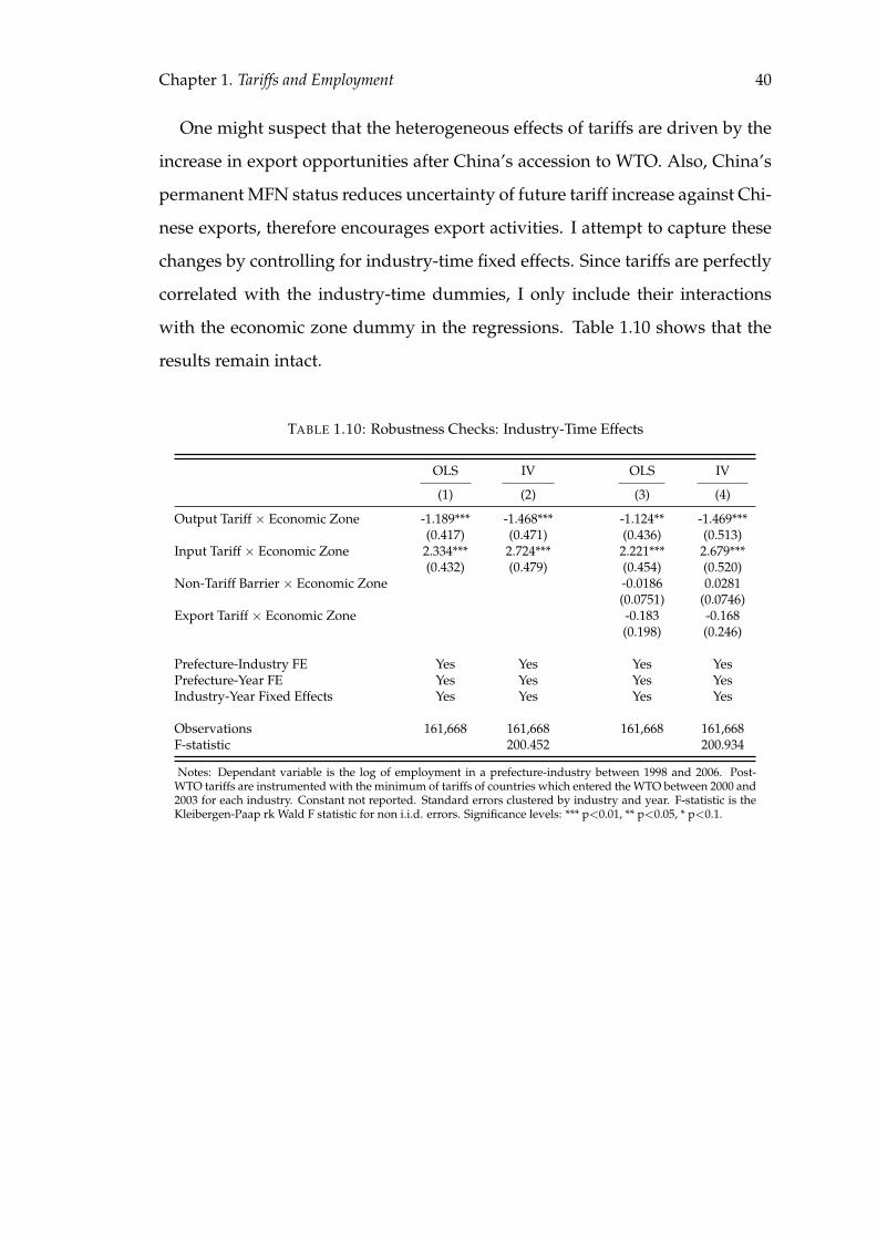
Chapter 1. Tariffs and Employment 40
One might suspect that the heterogeneous effects of tariffs are driven by the
increase in export opportunities after China’s accession to WTO. Also, China’s
permanent MFN status reduces uncertainty of future tariff increase against Chi-
nese exports, therefore encourages export activities. I attempt to capture these
changes by controlling for industry-time fixed effects. Since tariffs are perfectly
correlated with the industry-time dummies, I only include their interactions
with the economic zone dummy in the regressions. Table 1.10 shows that the
results remain intact.
TABLE 1.10: Robustness Checks: Industry-Time Effects
OLS IV OLS IV
(1) (2) (3) (4)
Output Tariff × Economic Zone -1.189*** -1.468*** -1.124** -1.469***(0.417) (0.471) (0.436) (0.513)
Input Tariff × Economic Zone 2.334*** 2.724*** 2.221*** 2.679***(0.432) (0.479) (0.454) (0.520)
Non-Tariff Barrier × Economic Zone -0.0186 0.0281(0.0751) (0.0746)
Export Tariff × Economic Zone -0.183 -0.168(0.198) (0.246)
Prefecture-Industry FE Yes Yes Yes YesPrefecture-Year FE Yes Yes Yes YesIndustry-Year Fixed Effects Yes Yes Yes Yes
Observations 161,668 161,668 161,668 161,668F-statistic 200.452 200.934
Notes: Dependant variable is the log of employment in a prefecture-industry between 1998 and 2006. Post-WTO tariffs are instrumented with the minimum of tariffs of countries which entered the WTO between 2000 and2003 for each industry. Constant not reported. Standard errors clustered by industry and year. F-statistic is theKleibergen-Paap rk Wald F statistic for non i.i.d. errors. Significance levels: *** p<0.01, ** p<0.05, * p<0.1.
Chapter 1. Tariffs and Employment 41
1.6.2 Other Outcomes
Apart from employment, I also consider the impact of tariff reduction on two
labour market outcomes: average wages and labour productivity.
Average wage of a prefecture-industry depends on the total demand of work-
ers and relative demand of different types of workers. Holding labour supply
constant, average wages increase if labour demand increases, and decreases
if labour demand decreases. Trade liberalisation also may affect the relative
demand of skilled workers. In our firm surveys, about 25% of the firms pro-
duce more than one type of product. Each product requires different skill mix.
Firms may change their product mix, and therefore worker’s composition, in
response to tariff cuts. When import competition is higher or imported inputs
are cheaper, firms may use labour more intensively and hire relatively more
unskilled workers to take advantage of the low labour cost in China. In this
case, the relative demand for unskilled workers increases and average wages
would decrease. Firms may also improve their product quality and increase
the relative demand for skilled labour if product quality is positively correlated
with worker’s skill level.20 If the relative demand for skilled workers increases,
then average wages would increase. So far our analysis is based on fixed labour
supply. If I relax this assumption and allow labour to move across regions and
sectors, the direction of adjustment would depend on the relative supply and
demand for each type of workers.
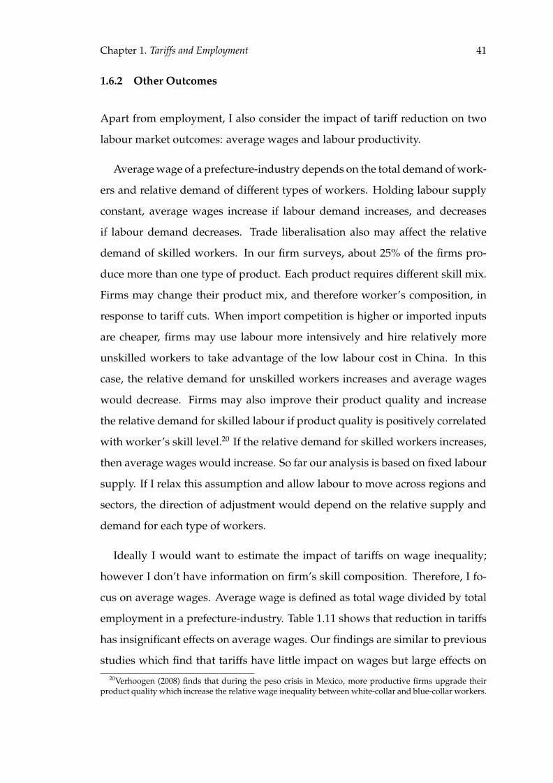
Ideally I would want to estimate the impact of tariffs on wage inequality;
however I don’t have information on firm’s skill composition. Therefore, I fo-
cus on average wages. Average wage is defined as total wage divided by total
employment in a prefecture-industry. Table 1.11 shows that reduction in tariffs
has insignificant effects on average wages. Our findings are similar to previous
studies which find that tariffs have little impact on wages but large effects on20Verhoogen (2008) finds that during the peso crisis in Mexico, more productive firms upgrade their
product quality which increase the relative wage inequality between white-collar and blue-collar workers.
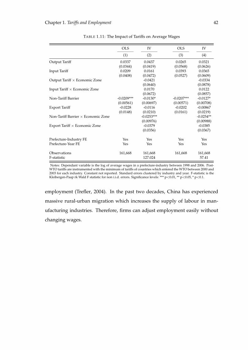
Chapter 1. Tariffs and Employment 42
TABLE 1.11: The Impact of Tariffs on Average Wages
OLS IV OLS IV
(1) (2) (3) (4)
Output Tariff 0.0337 0.0437 0.0265 0.0321(0.0344) (0.0419) (0.0568) (0.0626)
Input Tariff 0.0209 0.0161 0.0393 0.0365(0.0408) (0.0472) (0.0527) (0.0609)
Output Tariff × Economic Zone -0.0421 -0.0334(0.0640) (0.0878)
Input Tariff × Economic Zone 0.0170 0.0122(0.0672) (0.0857)
Non-Tariff Barrier -0.0209*** -0.0130* -0.0207*** -0.0127*(0.00561) (0.00697) (0.00571) (0.00708)
Export Tariff -0.0228 -0.0116 -0.0202 -0.00867(0.0148) (0.0210) (0.0161) (0.0219)
Non-Tariff Barrier × Economic Zone -0.0253*** -0.0254**(0.00976) (0.00988)
Export Tariff × Economic Zone -0.0379 -0.0385(0.0356) (0.0367)
Prefecture-Industry FE Yes Yes Yes YesPrefecture-Year FE Yes Yes Yes Yes
Observations 161,668 161,668 161,668 161,668F-statistic 127.024 57.41
Notes: Dependant variable is the log of average wages in a prefecture-industry between 1998 and 2006. Post-WTO tariffs are instrumented with the minimum of tariffs of countries which entered the WTO between 2000 and2003 for each industry. Constant not reported. Standard errors clustered by industry and year. F-statistic is theKleibergen-Paap rk Wald F statistic for non i.i.d. errors. Significance levels: *** p<0.01, ** p<0.05, * p<0.1.
employment (Trefler, 2004). In the past two decades, China has experienced
massive rural-urban migration which increases the supply of labour in man-
ufacturing industries. Therefore, firms can adjust employment easily without
changing wages.
Chapter 1. Tariffs and Employment 43
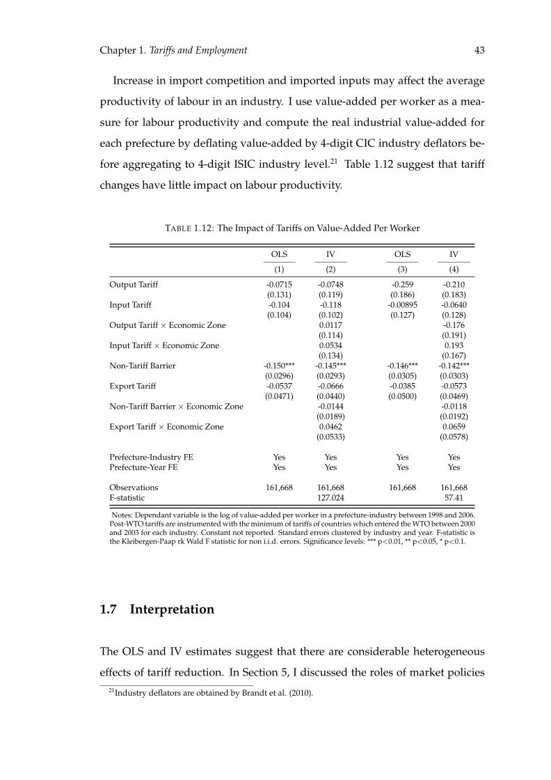
Increase in import competition and imported inputs may affect the average
productivity of labour in an industry. I use value-added per worker as a mea-
sure for labour productivity and compute the real industrial value-added for
each prefecture by deflating value-added by 4-digit CIC industry deflators be-
fore aggregating to 4-digit ISIC industry level.21 Table 1.12 suggest that tariff
changes have little impact on labour productivity.
TABLE 1.12: The Impact of Tariffs on Value-Added Per Worker
OLS IV OLS IV
(1) (2) (3) (4)
Output Tariff -0.0715 -0.0748 -0.259 -0.210(0.131) (0.119) (0.186) (0.183)
Input Tariff -0.104 -0.118 -0.00895 -0.0640(0.104) (0.102) (0.127) (0.128)
Output Tariff × Economic Zone 0.0117 -0.176(0.114) (0.191)
Input Tariff × Economic Zone 0.0534 0.193(0.134) (0.167)
Non-Tariff Barrier -0.150*** -0.145*** -0.146*** -0.142***(0.0296) (0.0293) (0.0305) (0.0303)
Export Tariff -0.0537 -0.0666 -0.0385 -0.0573(0.0471) (0.0440) (0.0500) (0.0469)
Non-Tariff Barrier × Economic Zone -0.0144 -0.0118(0.0189) (0.0192)
Export Tariff × Economic Zone 0.0462 0.0659(0.0533) (0.0578)
Prefecture-Industry FE Yes Yes Yes YesPrefecture-Year FE Yes Yes Yes Yes
Observations 161,668 161,668 161,668 161,668F-statistic 127.024 57.41
Notes: Dependant variable is the log of value-added per worker in a prefecture-industry between 1998 and 2006.Post-WTO tariffs are instrumented with the minimum of tariffs of countries which entered the WTO between 2000and 2003 for each industry. Constant not reported. Standard errors clustered by industry and year. F-statistic isthe Kleibergen-Paap rk Wald F statistic for non i.i.d. errors. Significance levels: *** p<0.01, ** p<0.05, * p<0.1.
1.7 Interpretation
The OLS and IV estimates suggest that there are considerable heterogeneous
effects of tariff reduction. In Section 5, I discussed the roles of market policies21Industry deflators are obtained by Brandt et al. (2010).
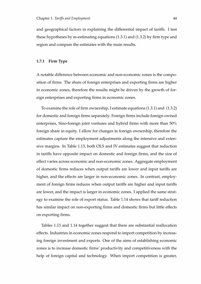
Chapter 1. Tariffs and Employment 44
and geographical factors in explaining the differential impact of tariffs. I test
these hypotheses by re-estimating equations (1.3.1) and (1.3.2) by firm type and
region and compare the estimates with the main results.
1.7.1 Firm Type
A notable difference between economic and non-economic zones is the compo-
sition of firms. The share of foreign enterprises and exporting firms are higher
in economic zones, therefore the results might be driven by the growth of for-
eign enterprises and exporting firms in economic zones.
To examine the role of firm ownership, I estimate equations (1.3.1) and (1.3.2)
for domestic and foreign firms separately. Foreign firms include foreign-owned
enterprises, Sino-foreign joint ventures and hybrid firms with more than 50%
foreign share in equity. I allow for changes in foreign ownership, therefore the
estimates capture the employment adjustments along the intensive and exten-
sive margins. In Table 1.13, both OLS and IV estimates suggest that reduction
in tariffs have opposite impact on domestic and foreign firms, and the size of
effect varies across economic and non-economic zones. Aggregate employment
of domestic firms reduces when output tariffs are lower and input tariffs are
higher, and the effects are larger in non-economic zones. In contrast, employ-
ment of foreign firms reduces when output tariffs are higher and input tariffs
are lower, and the impact is larger in economic zones. I applied the same strat-
egy to examine the role of export status. Table 1.14 shows that tariff reduction
has similar impact on non-exporting firms and domestic firms but little effects
on exporting firms.
Tables 1.13 and 1.14 together suggest that there are substantial reallocation
effects. Industries in economic zones respond to import competition by increas-
ing foreign investment and exports. One of the aims of establishing economic
zones is to increase domestic firms’ productivity and competitiveness with the
help of foreign capital and technology. When import competition is greater,
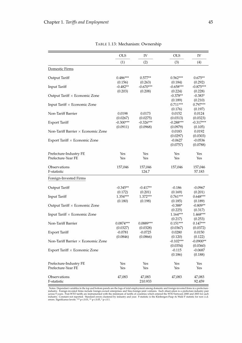
Chapter 1. Tariffs and Employment 45
TABLE 1.13: Mechanism: Ownership
OLS IV OLS IV
(1) (2) (3) (4)
Domestic Firms
Output Tariff 0.486*** 0.577** 0.562*** 0.675**(0.156) (0.263) (0.184) (0.292)
Input Tariff -0.482** -0.670*** -0.658*** -0.875***(0.203) (0.208) (0.224) (0.228)
Output Tariff × Economic Zone -0.378** -0.383*(0.189) (0.210)
Input Tariff × Economic Zone 0.711*** 0.797***(0.176) (0.197)
Non-Tariff Barrier 0.0198 0.0173 0.0152 0.0124(0.0267) (0.0275) (0.0313) (0.0323)
Export Tariff -0.300*** -0.326*** -0.288*** -0.317***(0.0911) (0.0968) (0.0979) (0.105)
Non-Tariff Barrier × Economic Zone 0.0183 0.0192(0.0297) (0.0303)
Export Tariff × Economic Zone -0.0627 -0.0536(0.0757) (0.0788)
Prefecture-Industry FE Yes Yes Yes YesPrefecture-Year FE Yes Yes Yes Yes
Observations 157,046 157,046 157,046 157,046F-statistic 124.7 57.183
Foreign-Invested Firms
Output Tariff -0.345** -0.417** -0.186 -0.0967(0.172) (0.201) (0.169) (0.201)
Input Tariff 1.354*** 1.372*** 0.761*** 0.648***(0.180) (0.198) (0.185) (0.189)
Output Tariff × Economic Zone -0.388* -0.809**(0.225) (0.317)
Input Tariff × Economic Zone 1.164*** 1.468***(0.217) (0.253)
Non-Tariff Barrier 0.0874*** 0.0889*** 0.151*** 0.147***(0.0327) (0.0328) (0.0367) (0.0372)
Export Tariff -0.0781 -0.0725 0.0280 0.0150(0.0846) (0.0866) (0.120) (0.122)
Non-Tariff Barrier × Economic Zone -0.102*** -0.0900**(0.0354) (0.0360)
Export Tariff × Economic Zone -0.115 -0.0687(0.186) (0.188)
Prefecture-Industry FE Yes Yes Yes YesPrefecture-Year FE Yes Yes Yes Yes
Observations 47,083 47,083 47,083 47,083F-statistic 210.933 92.459
Notes: Dependant variables in the top and bottom panels are the logs of total employment among domestic and foreign-invested firms in a prefecture-industry. Foreign-invested firms include foreign-owned enterprises and Sino-foreign joint ventures. Each observation is a prefecture-industry pairacross 9 years. Post-WTO tariffs are instrumented with the minimum of tariffs of countries which entered the WTO between 2000 and 2003 for eachindustry. Constant not reported. Standard errors clustered by industry and year. F-statistic is the Kleibergen-Paap rk Wald F statistic for non i.i.d.errors. Significance levels: *** p<0.01, ** p<0.05, * p<0.1.
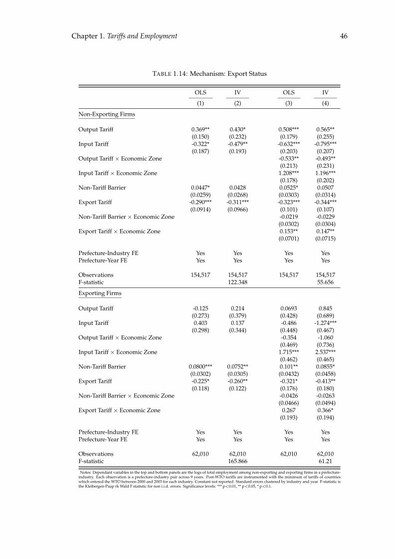
Chapter 1. Tariffs and Employment 46
TABLE 1.14: Mechanism: Export Status
OLS IV OLS IV
(1) (2) (3) (4)
Non-Exporting Firms
Output Tariff 0.369** 0.430* 0.508*** 0.565**(0.150) (0.232) (0.179) (0.255)
Input Tariff -0.322* -0.479** -0.632*** -0.795***(0.187) (0.193) (0.203) (0.207)
Output Tariff × Economic Zone -0.533** -0.493**(0.213) (0.231)
Input Tariff × Economic Zone 1.208*** 1.196***(0.178) (0.202)
Non-Tariff Barrier 0.0447* 0.0428 0.0525* 0.0507(0.0259) (0.0268) (0.0303) (0.0314)
Export Tariff -0.290*** -0.311*** -0.323*** -0.344***(0.0914) (0.0966) (0.101) (0.107)
Non-Tariff Barrier × Economic Zone -0.0219 -0.0229(0.0302) (0.0304)
Export Tariff × Economic Zone 0.153** 0.147**(0.0701) (0.0715)
Prefecture-Industry FE Yes Yes Yes YesPrefecture-Year FE Yes Yes Yes Yes
Observations 154,517 154,517 154,517 154,517F-statistic 122.348 55.656
Exporting Firms
Output Tariff -0.125 0.214 0.0693 0.845(0.273) (0.379) (0.428) (0.689)
Input Tariff 0.403 0.137 -0.486 -1.274***(0.298) (0.344) (0.448) (0.467)
Output Tariff × Economic Zone -0.354 -1.060(0.469) (0.736)
Input Tariff × Economic Zone 1.715*** 2.537***(0.462) (0.465)
Non-Tariff Barrier 0.0800*** 0.0752** 0.101** 0.0855*(0.0302) (0.0305) (0.0432) (0.0458)
Export Tariff -0.225* -0.260** -0.321* -0.413**(0.118) (0.122) (0.176) (0.180)
Non-Tariff Barrier × Economic Zone -0.0426 -0.0263(0.0466) (0.0494)
Export Tariff × Economic Zone 0.267 0.366*(0.193) (0.194)
Prefecture-Industry FE Yes Yes Yes YesPrefecture-Year FE Yes Yes Yes Yes
Observations 62,010 62,010 62,010 62,010F-statistic 165.866 61.21
Notes: Dependant variables in the top and bottom panels are the logs of total employment among non-exporting and exporting firms in a prefecture-industry. Each observation is a prefecture-industry pair across 9 years. Post-WTO tariffs are instrumented with the minimum of tariffs of countrieswhich entered the WTO between 2000 and 2003 for each industry. Constant not reported. Standard errors clustered by industry and year. F-statistic isthe Kleibergen-Paap rk Wald F statistic for non i.i.d. errors. Significance levels: *** p<0.01, ** p<0.05, * p<0.1.
Chapter 1. Tariffs and Employment 47
employment is reallocated to more productive firms in economic zones and, in
particular, to foreign enterprises. Firms also start exporting or increase export
intensity, thereby increase employment. This finding is consistent with a recent
work by Ma et al. (2012) which finds that Chinese manufacturing firms become
more labour-intensive when they export.
The employment effects of input tariffs in economic zones seem puzzling.
In Section 5, I argue that firm’s product type and technology determine the
degree of complementarity between labour and intermediate inputs, hence the
outcomes of input tariff reduction. Another reason is employment growth of
foreign enterprises and exporting firms is larger for industries which had lower
pre-WTO input tariffs, and these industries experienced little changes in input
tariffs after China’s accession to WTO.
1.7.2 Geographical Location
Our main results capture the joint effects of institutions and geographical fac-
tors on the outcomes of tariff reductions. To examine the role of geographical
factors, I run separate regressions for prefectures in the eastern and central-
western provinces. If the results are driven by geographical advantages, I should
not find significant differential impact across economic and non-economic zones
for each specification.
While 54% of the eastern prefecture-industries is located in economic zones,
only 4% of the central-western prefecture-industries is in economic zones. There-
fore, I expect insignificant heterogeneous effects in the central-western provinces.
In Table 1.15, I find that the tariff reduction have large effects in the eastern eco-
nomic zones and central-western non-economic zones. Two conclusions can be
drawn from the results. First, the differential impact of tariff cuts is not entirely
driven by geographical factors, although they do play an important role. Sec-
ond, compared to their eastern competitors, the effects of tariff reduction are
Chapter 1. Tariffs and Employment 48
larger in the central- western non-economic zones which are more geographi-
cally disadvantaged.
1.8 Conclusion
This paper studies the impact of trade liberalisation on regional manufactur-
ing employment in China and how this impact varies across regions with dif-
ferent market policies. After joining the WTO in 2001, China was required to
reduce tariffs significantly. While industries benefit from cheaper imported in-
puts, those which faced larger tariff cuts are subject to tougher import competi-
tion. I argue that the instrument variable strategies adopted in previous studies
to tackle the problem of tariff endogeneity are likely to fail the exogeneity as-
sumption if there are serial correlations in industry characteristics. I address
this concern by exploiting the exogeneity of WTO rules which are applied to
all member states. Our main results suggest that reduction in output and in-
put tariffs have insignificant impact on regional employment on average, and
this is due to the offsetting effects in economic and non-economic zones. For-
eign investment and export activities play an important role in the employment
adjustments in economic zones while geographical location partly explains the
results in non-economic zones. Our findings suggest that free-market system
and pro-trade policies affects the outcomes of market reforms. Countries which
didn’t gain from trade liberalisation might lack of the policies to protect local
companies during the initial period of opening or have insufficient incentives
to encourage the development of new capacity. How various economic policies
affect the outcomes of trade reforms are left for future research.
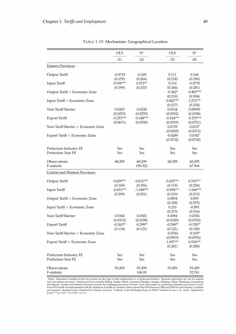
Chapter 1. Tariffs and Employment 49
TABLE 1.15: Mechanism: Geographical Location
OLS IV OLS IV
(1) (2) (3) (4)
Eastern Provinces
Output Tariff -0.0718 -0.249 0.111 0.164(0.159) (0.264) (0.218) (0.356)
Input Tariff 0.538*** 0.572** 0.110 -0.0770(0.199) (0.233) (0.264) (0.281)
Output Tariff × Economic Zone -0.362* -0.807***(0.210) (0.304)
Input Tariff × Economic Zone 0.842*** 1.272***(0.217) (0.234)
Non-Tariff Barrier 0.0203 0.0228 0.0124 0.00950(0.0253) (0.0255) (0.0332) (0.0338)
Export Tariff -0.253*** -0.248*** -0.244*** -0.270***(0.0671) (0.0700) (0.0703) (0.0751)
Non-Tariff Barrier × Economic Zone 0.0139 0.0237(0.0303) (0.0312)
Export Tariff × Economic Zone -0.0289 0.0347(0.0732) (0.0730)
Prefecture-Industry FE Yes Yes Yes YesPrefecture-Year FE Yes Yes Yes Yes
Observations 68,209 68,209 68,209 68,209F-statistic 150.322 67.564
Central and Western Provinces
Output Tariff 0.629*** 0.812*** 0.625*** 0.763***(0.169) (0.256) (0.174) (0.256)
Input Tariff -0.831*** -1.049*** -0.838*** -1.066***(0.209) (0.201) (0.210) (0.213)
Output Tariff × Economic Zone 0.0854 0.855(0.328) (0.575)
Input Tariff × Economic Zone 0.210 -0.583(0.373) (0.516)
Non-Tariff Barrier 0.0344 0.0302 0.0384 0.0354(0.0315) (0.0328) (0.0320) (0.0333)
Export Tariff -0.263** -0.299** -0.298** -0.328**(0.114) (0.121) (0.121) (0.128)
Non-Tariff Barrier × Economic Zone -0.0744 -0.103*(0.0553) (0.0576)
Export Tariff × Economic Zone 1.097*** 0.934***(0.281) (0.280)
Prefecture-Industry FE Yes Yes Yes YesPrefecture-Year FE Yes Yes Yes Yes
Observations 93,459 93,459 93,459 93,459F-statistic 106.93 52.761
Notes: Dependant variables in the two panels are the logs of total employment in a prefecture-industry. Separate regressions are run for easternand non-eastern provinces. Eastern provinces include Beijing, Tianjin, Hebei, Liaoning, Shanghai, Jiangsu, Zhejiang, Fujian, Shandong, Guangdongand Hainan. Central and Western Provinces include the remaining provinces in China. Each observation is a prefecture-industry pair across 9 years.Post-WTO tariffs are instrumented with the minimum of tariffs of countries which entered the WTO between 2000 and 2003 for each industry. Constantnot reported. Standard errors clustered by industry and year. F-statistic is the Kleibergen-Paap rk Wald F statistic for non i.i.d. errors. Significancelevels: *** p<0.01, ** p<0.05, * p<0.1.
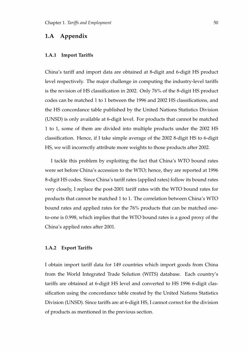
Chapter 1. Tariffs and Employment 50
1.A Appendix
1.A.1 Import Tariffs
China’s tariff and import data are obtained at 8-digit and 6-digit HS product
level respectively. The major challenge in computing the industry-level tariffs
is the revision of HS classification in 2002. Only 76% of the 8-digit HS product
codes can be matched 1 to 1 between the 1996 and 2002 HS classifications, and
the HS concordance table published by the United Nations Statistics Division
(UNSD) is only available at 6-digit level. For products that cannot be matched
1 to 1, some of them are divided into multiple products under the 2002 HS
classification. Hence, if I take simple average of the 2002 8-digit HS to 6-digit
HS, we will incorrectly attribute more weights to those products after 2002.
I tackle this problem by exploiting the fact that China’s WTO bound rates
were set before China’s accession to the WTO; hence, they are reported at 1996
8-digit HS codes. Since China’s tariff rates (applied rates) follow its bound rates
very closely, I replace the post-2001 tariff rates with the WTO bound rates for
products that cannot be matched 1 to 1. The correlation between China’s WTO
bound rates and applied rates for the 76% products that can be matched one-
to-one is 0.998, which implies that the WTO bound rates is a good proxy of the
China’s applied rates after 2001.
1.A.2 Export Tariffs
I obtain import tariff data for 149 countries which import goods from China
from the World Integrated Trade Solution (WITS) database. Each country’s
tariffs are obtained at 6-digit HS level and converted to HS 1996 6-digit clas-
sification using the concordance table created by the United Nations Statistics
Division (UNSD). Since tariffs are at 6-digit HS, I cannot correct for the division
of products as mentioned in the previous section.
Chapter 1. Tariffs and Employment 51
I am able to obtain complete tariff data from China’s major trading part-
ners such as EU, US, Japan and South Korea. However, less than 10% of the
remaining countries report tariffs every year between 1998 and 2006. To con-
struct China’s export tariffs, I replace missing observations with the following
assumptions: First, if the first year for which data is available is after 1998, then
the tariff rates before are the same as the rates in the first year of reporting.
Second, if the last data year is before 2006, then the tariff rates afterwards are
the same as the last year of reporting. Third, tariffs missing between 2 years
are assumed to change in equal installments. After replacing the missing val-
ues, I aggregate the tariff data up to 4-digit ISIC level using the country-import
shares of China in 1998. The problem of this approach is it tends to smooth tar-
iff changes across years and won’t capture the possible sharp drop in China’s
export tariffs in 2002. However, this shouldn’t introduce a large bias to my esti-
mates since the total change in tariff rates between 1998 and 2006 is quite small.
Any drop in export tariffs in 2002 has to be offset by a large increase afterwards,
which is unlikely to happen.
1.A.3 Economic Zones in China
Chapter 1. Tariffs and Employment 52
TABLE 1.16: List of Prefectures with Economic Zones Before 2000
National EconomicSpecial Coastal Coastal and Technological
Province Prefecture Economic Zone Open City Economic Zone Development Zone
Anhui Wuhu 1993Beijing Beijing 1994Chongqing Chongqing 1993Fujian Fuzhou 1984 1985Fujian Shantou 1980Fujian Xiamen 1980 1989Fujian Zhangzhou 1993Guangdong Dongguan 1994Guangdong Foshan 1994Guangdong Guangzhou 1984 1994 1984Guangdong Huizhou 1993Guangdong Jiangmen 1994Guangdong Shenzhen 1980 1994Guangdong Zhanjiang 1984 1984Guangdong Zhongshan 1994Guangdong Zhuhai 1980 1994Guangxi Beihai 1984Hainan All Prefectures 1988Hebei Qinhuangdao 1984 1984Heilongjiang Harbin 1993Jiangsu Changzhou 1992Jiangsu Lianyungang 1984 1984Jiangsu Nanjing 1992Jiangsu Nantong 1984 1984Jiangsu Suzhou 1992 1992Jiangsu Taizhou 1992Jiangsu Wuxi 1992Jiangsu Zhenjiang 1992Jilin Changchun 1993Liaoning Dalian 1984 1984Liaoning Shengyang 1993Liaoning Yingkou 1992Shandong Qingdao 1984 1984Shandong Weihai 1992Shandong Yantai 1984 1984Shanghai Shanghai 1984 1992 1986Tianjin Tianjin 1984 1984Xinjiang Urumqi 1994Zhejiang Hangzhou 1992 1993Zhejiang Huzhou 1992Zhejiang Jiaxing 1992Zhejiang Ningbo 1984 1992 1984Zhejiang Shaoxing 1992Zhejiang Wenzhou 1984 1992Zhejiang Zhoushan 1992
Notes: Numbers in the table are the years of establishment of economic zones. Source: Ministry of Commerce

Chapter 2
Productivity As If Space Mattered:
An Application to Factor Markets
Across China
2.1 Introduction
A number of studies document large and persistent differences in productiv-
ity across both countries and firms.1 However, these differences remain largely
‘some sort of measure of our ignorance’ (Abramovitz, 1956). This paper in-
quires to what extent the supply characteristics of regional input markets might
help explain such systematic productivity dispersion across firms. It would be
surprising if disparate factor markets result in similar outcomes, when clearly
the prices and quality of inputs available vary considerably. Modelling firm
adaptation to different factor markets provides insights and testable predictions
about how firms produce and where they choose to locate.
Differences between factor markets, especially for labour, are likely to be es-
pecially stark in developing economies undergoing urbanisation (Lewis, 1954),
or when government policies increase relocation costs beyond those normally1See Syverson (2011) for a review.
53
Chapter 2. Productivity As If Space Mattered 54
present.2 Even the US labour market, which is considered relatively fluid, ex-
hibits high migration costs as measured by the wage differential required to
drive relocation (Kennan and Walker, 2011). Thus, free movement of factors
does not mean frictionless movement, and recent work has indicated imper-
fect factor mobility has sizable economic effects (Topalova, 2010). Rather than
considering the forces which cause workers to locate across space, this paper
instead takes a different turn to inquire what existing differences in regional
input markets imply for firm input use, productivity and location.
Although there might be many complementary ways to address our ques-
tion, we take an approach rooted in the general equilibrium trade literature to
understand how local endowments impact firms which enter endogenously, as
typified by Bernard et al. (2007). We extend their model to incorporate entry
across regional markets and richer employment structures. Each region is en-
dowed with a different distribution of skill types and wages across workers.
Industries vary in team technology, which is their ability to substitute between
different types of labour (e.g. Bowles, 1970). Firms hire teams of workers by
choosing the optimal combination of workers given local conditions. Since each
firm’s optimal labour force varies by industry technology and region, the com-
parative suitability of regions varies by industry. Firms thus locate in propor-
tion to the cost advantages available.
In the model, finding new employees entails fixed costs and the ease of find-
ing any type of worker increases with their regional supply. Therefore firm hir-
ing depends on the joint distribution of worker types and wages. Since labour
demand depends on technology and regional labour markets, this implies effec-
tive labour costs vary by region and industry. These labour costs help explain
differences in productivity.3 But are these differences economically important?2Institutional mobility constraints, such as the hukou system in China, likely further exacerbate differ-
ences.3Effective labour costs are driven by the complementarity of regional endowments with industry tech-
nology, and the paper refers to these additional real production possibilities as ‘productivity’.
Chapter 2. Productivity As If Space Mattered 55
To quantify real world supply conditions, we use the model to derive estimat-
ing equations which fix: 1) hiring by wage and worker type distributions, 2)
substitution into non-labour inputs, and 3) firm location in response to local
factor markets.
The estimation strategy combines manufacturing and population census data
for China in the mid-2000s, a setting which exhibits substantial variation in
labour market conditions. By revealing how firm demand for skills varies with
local conditions, the model allows recovery of the unit costs for labour across
China. Our estimates imply an interquartile difference in effective labour costs
of 30 to 80 percent. A second stage estimates production functions, explicitly
accounting for regional cost differences. Since firms are capable of substitut-
ing into non-labour inputs, productivity differences are smaller than labour
cost differences. Once substitution is accounted for, labour costs result in firm
productivity differences of 3 to 17 percent, and explain 4 to 43 percent of the
variance of productivity.4 Furthermore, we show that economic activity locates
where regional costs are lowest, as implied by the model.
We conclude this section by relating the paper to existing work. The pa-
per then continues by laying out a model that incorporates a rich view of the
labour hiring process. The model explains how firms internalize local labour
market conditions to maximize profits, resulting in an industry specific unit
cost of labour by region. Section 3 places these firms in a general equilibrium,
monopolistic competition framework, in particular addressing the determina-
tion of factor prices and firm location. Section 4 explains how the model can
be estimated with a simple nested OLS approach. Section 5 discusses details
of the data, while Section 6 presents our model estimates and uses them to ex-
plain the effect of different regional input markets on firm behaviour. Section 7
concludes.4These substantial differences underscore Kugler and Verhoogen (2011): since TFP is often the ‘primary
measure of [...] performance’, accounting for local factor markets might substantially alter estimates ofpolicy effects.
Chapter 2. Productivity As If Space Mattered 56
Our consideration of firms as dependent on local factor markets is based
on models typified by the Heckscher-Ohlin-Vanek theory of international trade
(e.g. Vanek, 1968). The departures from H-O-V in our model relax assumptions
about perfect labour substitutability and homogeneous factor markets, which
quantifies the role of local labour markets. On the product market side, we con-
sider many goods as indicated by Bernstein and Weinstein (2002) as appropriate
when considering the locational role of factor endowments. We follow a multi-
sector approach similar to Melitz (2003), but add free entry by firms across re-
gions. A firm’s optimal location depends on local costs which arise from the
regional distribution of worker types and wages, but competition from firms
which enter the same region prevent complete specialisation. The model quan-
tifies the intensity of firm entry and shows that within country, advantageous
local factor markets are important for understanding specialisation patterns.5
Recently, both Borjas (2009) and Ottaviano and Peri (2010) have emphasized
the importance of more complete model frameworks to estimate substitution
between worker types. In distinction to the labour literature, our interest is firm
substitution across factor markets. Dovetailing with this are theories proposing
that different industries perform optimally under different degrees of skill di-
versity. Grossman and Maggi (2000) build a theoretical model explaining how
differences in skill dispersion across countries could determine comparative ad-
vantage and global trade patterns. Building on this work, Morrow (2010) mod-
els multiple industries and general skill distributions, and finds that skill diver-
sity is explains productivity and export differences in developing countries.
The importance of local market characteristics, especially in developing coun-
tries, has recently been emphasized by Karadi and Koren (2012). These authors
calibrate a spatial firm model to sector level data in developing countries to
better account for the role of firm location in measured productivity. Moretti5In spirit, this result is akin to Fitzgerald and Hallak (2004) who study the role of cross country pro-
ductivity differences in specialisation. In our case, differences in unit labour costs predict specialisationacross regions.
Chapter 2. Productivity As If Space Mattered 57
(2011) reviews work on local labour markets and agglomeration economies, ex-
plicitly modelling spatial equilibrium across labour markets. Distinct from this
literature, we take the outcome of spatial labour markets as given and focus on
the trade-offs firms face and the consequences of regional markets on effective
labour costs and firm location.6,7
Although we are unaware of other studies estimating model primitives as
a function of local market characteristics, reduced form empirical work is con-
sonant with the theoretical implications. Iranzo et al. (2008) find that higher
skill dispersion is associated with higher TFP in Italy. Similarly, Parrotta et al.
(2011) find that diversity in education leads to higher productivity in Denmark.
Martins (2008) finds that firm wage dispersion affects firm performance in Por-
tugal. Bombardini et al. (2012) use literacy scores to show that countries with
more dispersed skills specialize in industries characterized by lower skill com-
plementarity. In contrast, this paper combines firm and population census data
to explicitly model regional differences, leading to micro founded identification
and estimates. The method used is novel, and results of this paper highlight the
degree to which firm behaviour are influenced through the availability of inputs
at the micro level.8
Clearly this study also contributes to the empirical literature on Chinese pro-
ductivity. Ma et al. (2012) show that exporting is positively correlated with TFP
and that firms self select into exporting which, ex post, further increases TFP.
Brandt et al. (2012) estimate Chinese firm TFP, showing that new entry accounts
for two thirds of TFP growth and that TFP growth dominates input accumula-
tion as a source of output growth. Hsieh and Klenow (2009) posit that India and6Several papers have explored how different aspects of labour affect firm-level productivity. There
is substantial work on the effect of worker skills on productivity (Abowd Kramarz and Margolis (1999,2005), Fox and Smeets (2011)). Other labour characteristics that drive productivity include managerialtalent and practices (Bloom and van Reenen, 2007), social connections among workers (Bandiera et al.,2009), organisational form (Garicano and Heaton, 2010) and incentive pay (Lazear, 2000).
7Determinants of productivity include market structure (Syverson (2004)), product market rivalry andtechnology spillovers (Bloom et al. (2007)) and vertical integration (Horta and Syverson (2007), Atalayet al. (2012)).
8The importance of backward linkages for firm behaviour are a recurring theme in both the develop-ment and economic geography literature, see Hirschman (1958) and recently Overman and Puga (2010).
Chapter 2. Productivity As If Space Mattered 58
China have lower productivity relative to the US due to resource misallocation
and compute how manufacturing TFP in India and China would increase if re-
source allocation was similar to that of the US. This paper uncovers local factors
that determine productivity. How this interacts with the above mechanisms is
a potential area for further work.9
2.2 The Role of Skill Mix in Production
This section develops a model of hiring in which firms respond to both the
wages and quantities of locally available worker types. Firms combine homo-
geneous inputs (materials, capital) and differentiated inputs (types of labour).
While homogeneous inputs are perfectly mobile within industries, we take the
distribution of labour endowments as given. Special cases of our model would
include perfect factor mobility (equal endowments in all regions) or high mi-
gration costs (equalisation up to mobility costs). Industries have different tech-
nologies available for combining types of labour into teams. We proceed with a
detailed specification of the labour hiring process, solving for firms’ optimal re-
sponses to local labour market supply conditions. This quantifies the unit cost
for labour by region in terms of observable local conditions and model param-
eters.
2.2.1 Firm Production
Firms within an industry T face a neoclassical production technologyF T (M,K,L)
which combines materials M , capital K and labour L to produce output. An
industry specific capital stock KT is mobile within each industry, and in equi-
librium is available at rental rate rTK . Similarly, an industry specific stock of ma-
terials MT is mobile and available at price rTM . While M and K are composed9Such regional differences might help explain the Chinese export facts of Manova and Zhang (2012)
and the different impact of liberalisation across trade regimes found by Bas and Strauss-Kahn (2012).
Chapter 2. Productivity As If Space Mattered 59
of homogeneous units, effective labour L is produced by combining heteroge-
neous worker types.
There are S skill types of workers which are distributed unequally across re-
gionsR. The distribution of worker types in regionR is denoted aR = (aR,1, . . . , aR,S).
The regional wages for each type are take as exogenous by workers and firms,
and in equilibrium are denote wR = (wR,1, . . . , wR,S). Workers do not contribute
equally to output. This occurs for two reasons. First, each type provides an in-
dustry specific level of human capital mTi . Second, when a worker meets a firm,
this match has a random quality h ≥ 1 which follows a Pareto distribution,
Ψ (h) ≡ 1− h−k.
In order to hire workers, a firm must pay a fixed search cost of f effective
labour units, at which point they may hire from a distribution of worker types
aR. The firm hires on the basis of match quality, and consequently chooses
a minimum threshold of match quality for each type they will retain, h =
(h1, . . . , hS).10 Upon keeping a preferred set of workers, the firm may this pro-
cess N times until achieving their desired workforce. At the end of hiring, the
amount of human capital produced by each type i is given by
Hi ≡ N · aR,imTi
∫ ∞hi
hdΨ. (2.2.1)
From a firm’s perspective, the threshold of worker match quality h is a means to
choose an optimal level of H . However, as a firm lowers its quality threshold,
it faces an increasing average cost of each type of human capital Hi . These
increasing average costs induce the firm to maintain hi ≥ 1 and to increase N
to search harder for suitable workers.10This assumption is familiar from labour search models (see Helpman et al. (2010a)). Unlike Helpman,
et al., here differences in hiring patterns are determined by local market conditions.
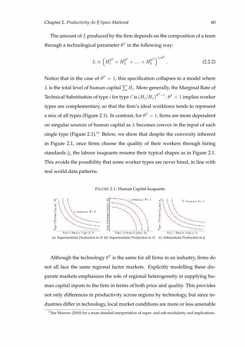
Chapter 2. Productivity As If Space Mattered 60
The amount of L produced by the firm depends on the composition of a team
through a technological parameter θT in the following way:
L ≡(HθT
1 +HθT
2 + . . .+HθT
S
)1/θT. (2.2.2)
Notice that in the case of θT = 1, this specification collapses to a model where
L is the total level of human capital∑Hi. More generally, the Marginal Rate of
Technical Substitution of type i for type i′ is (Hi/Hi′)θT−1. θT < 1 implies worker
types are complementary, so that the firm’s ideal workforce tends to represent
a mix of all types (Figure 2.1). In contrast, for θT > 1, firms are more dependent
on singular sources of human capital as L becomes convex in the input of each
single type (Figure 2.1).11 Below, we show that despite the convexity inherent
in Figure 2.1, once firms choose the quality of their workers through hiring
standards h, the labour isoquants resume their typical shapes as in Figure 2.1.
This avoids the possibility that some worker types are never hired, in line with
real world data patterns.
FIGURE 2.1: Human Capital Isoquants
(a) Supermodular Production in H (b) Supermodular Production in H (c) Submodular Production in h
Although the technology θT is the same for all firms in an industry, firms do
not all face the same regional factor markets. Explicitly modelling these dis-
parate markets emphasizes the role of regional heterogeneity in supplying hu-
man capital inputs to the firm in terms of both price and quality. This provides
not only differences in productivity across regions by technology, but since in-
dustries differ in technology, local market conditions are more or less amenable11See Morrow (2010) for a more detailed interpretation of super- and sub-modularity and implications.
Chapter 2. Productivity As If Space Mattered 61
to particular industries. We now detail the hiring process, introducing different
markets and deriving firms’ optimal hiring to best accommodate these differ-
ences.
2.2.2 Unit Labour Costs by Region and Technology
The total costs of hiring labour depend on the regional wage rates wR, the avail-
ability of workers aR, and the unit cost of labour in region R using technology
T , labelled cTR. Since the total number of each type i hired is NaR,i (1−Ψ (hi)),
the total hiring bill is
Total Hiring Costs : N
[∑i
wR,iaR,i (1−Ψ (hi)) + fcTR
]. (2.2.3)
To produce a given vector (H1, . . . , HS), the firm faces a trade-off between the
quantity and quality of workers hired. For instance, the firm might hire a large
number of workers and “cherry pick” the best matches by choosing high values
for h. Alternatively, the firm might save on interviewing costs f by choosing a
low number of prospectives N and permissively low values for h. Local trade
offs and the dependence on the regional labour supply characteristics aR andwR
is made explicit by considering the technology and region specific cost function
CT (H|aR, wR), defined by
CT ≡ minN,h
N
[∑i
aR,iwR,i (1−Ψ (hi)) + fcTR
]where Hi = NaR,im
Ti
∫ ∞hi
hdΨ ∀i.
(2.2.4)
Letting µi denote the Lagrange multiplier for each of the S cost minimisation
constraints, the first order conditions for {hi} imply µi = wR,i/mTi hi, while the
choice of N implies
CT (H|aR, wR) =∑i
µiHi = N∑
wR,iaR,i
∫ ∞hi
h/hidΨ. (2.2.5)
Chapter 2. Productivity As If Space Mattered 62
Equation (2.2.5) shows that the multipliers µi are the marginal cost contribution
(per skill unit) toHi of the last type iworker hired. The cost functionCT implies
the unit labour cost of L in region R is
Unit Labour Cost Problem : cTR ≡ minH
CT (H|aR, wR) subject to L = 1. (2.2.6)
The unit labour cost function may be solved as
Unit Labour Costs : cTR =
[∑i hired
[aR,i
(mTi
)kw1−k
R,i /f (k − 1)]θT /βT](βT /θT )/(1−k)
.
(2.2.7)
The trade off between being more selective (high h) and avoiding search costs
(fcTR) is clearly illustrated by combining Equations (2.2.3) and (2.2.5), which
shows:
∑i
aR,iwR,i
∫ ∞hi
(h− hi) /hidΨ= fcTR. (2.2.8)
The LHS of Equation (2.2.8) decreases in h, so when a firm faces lower inter-
viewing costs it can afford to be more selective by increasing h. Conversely, in
the presence of high interviewing costs, the firm optimally “lowers their stan-
dards” h to increase the size of their workforce without interviewing additional
workers.12
2.2.3 Optimal Hiring Patterns
The above reasoning shows the relationship between technology and the opti-
mal choice of worker types. It is intuitive that if the right tail of the match qual-
ity distribution is sufficiently thick, there are a few excellent matches for each12The number of times a firm goes to hire workers,N , can be solved asN = 1/fk. Thus,N is decreasing
in both hiring costs and k. Increases in k imply lower match quality, so that repeatedly screening workershas lower returns.
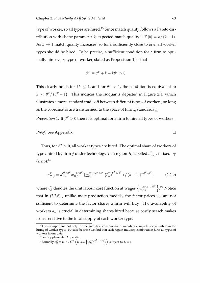
Chapter 2. Productivity As If Space Mattered 63
type of worker, so all types are hired.13 Since match quality follows a Pareto dis-
tribution with shape parameter k, expected match quality is E [h] = k/ (k − 1).
As k → 1 match quality increases, so for k sufficiently close to one, all worker
types should be hired. To be precise, a sufficient condition for a firm to opti-
mally hire every type of worker, stated as Proposition 1, is that
βT ≡ θT + k − kθT > 0.
This clearly holds for θT ≤ 1, and for θT > 1, the condition is equivalent to
k < θT/(θT − 1
). This induces the isoquants depicted in Figure 2.1, which
illustrates a more standard trade off between different types of workers, so long
as the coordinates are transformed to the space of hiring standards h.
Proposition 1. If βT > 0 then it is optimal for a firm to hire all types of workers.
Proof. See Appendix.
Thus, for βT > 0, all worker types are hired. The optimal share of workers of
type i hired by firm j under technology T in region R, labelled sTR,ij , is fixed by
(2.2.6):14
sTR,ij = aθT /βT
R,i w−k/βTR,i
(mTi
)kθT /βT
(cTR)θT k/βT
(f (k − 1))−θT /βT . (2.2.9)
where cTR denotes the unit labour cost function at wages{wk/(k−1)θTR,i
}.15 Notice
that in (2.2.6) , unlike most production models, the factor prices wR are not
sufficient to determine the factor shares a firm will buy. The availability of
workers aR is crucial in determining shares hired because costly search makes
firms sensitive to the local supply of each worker type.13This is important, not only for the analytical convenience of avoiding complete specialisation in the
hiring of worker types, but also because we find that each region-industry combination hires all types ofworkers in our data.
14See Supplemental Appendix.15Formally cTR ≡ minH C
T(H|aR,
{w−k/θT (1−k)R,i
})subject to L = 1.
Chapter 2. Productivity As If Space Mattered 64
2.2.4 Unit Costs: The Role of Substitution
Equation (2.2.7) summarizes the cost of one unit of labour L in terms of the
Pareto shape parameter k, the technology θT and regional characteristics aR and
wR. In order to solve for total unit costs (which include non-labour costs), we
assume each production function F T is of a Cobb-Douglas form with constant
returns to scale:
F T (M,K,L) = MαTMKαTKLαTL . (2.2.10)
It is then straightforward to derive total unit costs from (2.2.7) and (2.2.10) as
Total Unit Costs : uTR =(rTM/α
TM
)αTM (rTK/αTK)αTK (cTR/αTL)αTL , (2.2.11)
where uTR represents the regional component of unit costs for industry T in re-
gion R. Within an industry, productivity then varies across regions as in the
following example: if firm 1 in region R and firm 2 in region R′ face unit labour
costs of cTR and cTR′ and have the same wage bill W , they will employ labour
of L1 = W/cTR and L2 = W/cTR′ . Thus, if these firms hire the same capital and
material inputs (K,M), then the ratio of their output is
Y 1/Y 2 =(MαTMKαTKL
αTL1
)/(MαTMKαTKL
αTL2
)= (L1/L2)
αTL =(cTR′/c
TR
)αTL .Industry differences in productivity therefore depend on 1) the ratio of regional
labour costs and 2) the intensity αTL of labour in production. Estimating both
allows quantification of regional productivity differences. However, we first
resolve factor prices and firm location in general equilibrium.
Chapter 2. Productivity As If Space Mattered 65
2.3 Firm Production under Monopolistic Competition
This section combines the insights into firm behaviour just developed into a
general equilibrium model of monopolistic competition. Firms, who are ex ante
identical, choose among regions to locate. Key to a firm’s location decision are
the expected profits of entry. These profits depend on 1) the distribution of
worker types and wages and 2) the competition present from other firms who
enter the region. We characterize production and location choices conditional
on local labour markets. Most strikingly, lower regional production costs at-
tract more firms for any given technology, which determines the intensity of
economic activity. Furthermore, we show an equilibrium wage vector exists
which supports these choices by firms for any distribution of labour endow-
ments. Thus, endowment distributions as implied by complete labour mobility
or migration models are consistent with our framework.
2.3.1 Firms and Consumers
Each region R is endowed with a population PR composed of S worker types.
Firms may enter any region R by paying a sunk entry cost Fe. Firms then re-
ceive a random cost draw ηj ∼ G and face a fixed production cost fe.16 Akin to
Bernard et al. (2007), firms combine different types of inputs to produce. Each
firm j produces a distinct variety, and in equilibrium a mass of firms MTR enter.
Entrants with cost draws less than a prohibitively high cost level ηTR produce.
MTR and ηTR together determine the set of varieties available to consumers.
Consumer preferences over varieties j and quantities{QTRj
}take the Dixit-
Stiglitz form
UTR ≡ U
(MT
R, ηTR, Q
TR
)= MT
R
∫ ηTR
0
(QTRj
)ρdG (j)
16This follows Melitz (2003). G is assumed to be absolutely continuous with finite mean.
Chapter 2. Productivity As If Space Mattered 66
in each region and industry, with total utilityU (M, η, Q) ≡ ΠTΠR
(UTR
)σTR , where
σTR are relative weights put on final goods normalized so that∑
T,R σTR = 1. As
shown in the Appendix, each σTR has the usual interpretation as the share of
income spent on goods from each region and technology pair (R, T ).17
Firms are the sole sellers of their variety, and thus are monopolists who pro-
vide their variety at a price P TRj . Consumers, in turn, face a vector of prices{
P TRj
}, and a particular consumer with income I has the following demand
curve for each variety:
QTRj = I ·
(P TRjU
TR/σ
TR
) 1ρ−1 /
∑t,r
(σtr) 1ρ−1 Mt
r
∫ ηtr
0
((P tr,z
)ρU tr
) 1ρ−1 dG (z) . (2.3.1)
Clearly, even if consumers have different incomes, aggregate demand for va-
riety j corresponds to that of a representative consumer with income equal to
aggregate income, IAgg. Since labour is supplied inelastically, IAgg is necessarily
IAgg =∑R
∑i
wR,iaR,iPR︸ ︷︷ ︸Total Wages of Type i in R
+∑T
rTMMT + rTKK
T︸ ︷︷ ︸Non−labour Income
. (2.3.2)
After paying an entry cost of Fe output units, firms know their cost draw,
which paired with regional input markets determine their total unit cost uTR.
Firms maximize profits
πTRj(P TRj
)=(P TRj − uTRηj
)QTRj − uTRfe
by choosing an optimal price P TRj = uTRηj/ρ, resulting in a markup of 1/ρ over
costs. Firms who cannot make a positive profit do not produce to avoid pay-
ing the fixed cost of fe output units. Since profits decrease in costs, there is a
unique cutoff cost draw ηTR which implies zero profits, while firms with ηj < ηTR
produce. As there are no barriers to entry besides the entry cost Fe, firms enter17Note that since the demand for goods from each (R, T ) pair enter preferences multiplicatively, com-
plete specialisation cannot occur which considerably simplifies the analysis.
Chapter 2. Productivity As If Space Mattered 67
in every region until expected profits are zero. This yields the
Spatial Zero Profit Condition : E[πTRj]
= Fe, ∀R, T.
It is shown in the Appendix that the cutoff cost draw ηTR depends only on fe, Fe,
and G, so there is a unique cutoff cost that does not vary by region or industry.
Having determined firm behaviour in the product market, we now examine
input markets.
2.3.2 Regional Factor Market Clearing
The remaining equilibrium conditions are that input prices guarantee firm in-
put demand exhausts materials, capital stocks, and each regional pool of work-
ers. To fix expenditure, we assume each budget share σTR is proportional to PR,
so that σTR = σTPR for some σT .18 Since production is Cobb-Douglas, the share
of total costs (equal to IAgg) which go to each factor is the factor output elasticity,
so full resource utilisation of materials and capital requires
MT = αTMσT IAggP/rTM , KT = αTKσ
T IAggP/rTK . (2.3.3)
where P ≡∑
R PR is the total population. These two equations capture the
allocation of technology specific resources across regions.
In contrast, effective labour of LTR is produced by each technology in each
region. Since the wage bill LTRcTR must receive a share αTL of total revenues,
Aggregate Labour Demand : LTR = αTLσT IAggPR/cTR. (2.3.4)
Embedded in each LTR is the set of workers hired by firms attendant to regional
market conditions. The total demand for employees of each type in region R
18This assumption is justified by the implication that two regions which have identical skill distributionshave the same wage schedule.
Chapter 2. Productivity As If Space Mattered 68
implied by Equation (2.2.9) must equal the supply of aR,iPR, yielding the re-
gional resource clearing conditions. Wages are therefore determined by
aR,iwR,i =∑T
σT︸︷︷︸Industry Share Per Capita
· αTL︸︷︷︸Labour Share
·HθT
R,i/ΣjHθT
R,j︸ ︷︷ ︸Type Share
·IAgg ∀R, i. (2.3.5)
Equation (2.3.5) shows that type i’s contribution to mean wages, aR,iwR,i, is the
sum over income spent an industry, times labour’s share, times the wages at-
tributable to each type.19
Solving Equation (2.3.5) requires finding a wage for each worker type in each
region that fully employs all workers. To do so, first note that the resource clear-
ing conditions determine wages, provided an exogenous vector of unit labour
costs{cTR}
, proved in the Appendix:
Lemma. There is a wage function W that uniquely solves (2.3.5) given unit labour
costs.
Of course, unit labour costs are not exogenous as in the Lemma, but rather
depend on endogenous wages {wR,i}. However, the lemma does show that the
following mapping:
{wR,i} 7→Equation 2.2.7
{cTR ({wR,i})
}7→
LemmaW({cTR ({wR,i})
}),
which starts at one wage vector {wR,i} and ends at another wage vector W is
well defined. This mapping is shown in the Appendix to have a fixed point,
which implies
Proposition 2. An equilibrium wage vector exists which clears each regional labour
market.19In equilibrium, the type share is
HθT
R,i/ΣjHθT
R,j =(aR,i
(mTi
)kw1−k
R,i
)θT /βT
/Σj(aR,j
(mTj
)kw1−k
R,j
)θT /βT
Chapter 2. Productivity As If Space Mattered 69
2.3.3 Limited Factor Price Equalisation
Since workers are imperfectly substitutable, they induce spillovers within firms,
and consequently are not paid their marginal product.20 Mirroring this, the
equation for unit labour costs shows that regions with different skill distribu-
tions, say region R and R′, typically cannot have both cTR = cTR′ and wR = wR′ .
However, factor price equalisation for labour holds in a limited fashion in two
ways. First, Equation (2.3.4) shows the industry wage bill per capita is equalized,
formally
cTRLTR/PR = cTR′L
TR′/PR′ for all region pairs (R,R′) .
Second, summing across types in (2.3.5) implies
Average Wages :∑i
aR,iwR,i =∑T
αTLσT IAgg,
so average wages are constant across regions. This is summarized as
Proposition 3. Average wages are equalized across regions.
Proposition 3 shows that while our model allows for heterogeneity of wages
by worker type, general equilibrium forces still imply that factor price equali-
sation holds on average.
2.3.4 Regional Specialisation of Firms
Of course, differences in input costs will influence the relative concentration of
firms across regions. Since regions may vary substantially in population size
P, the most relevant metric is the number of firms per capita, MTR · G
(ηTR)/PR.
The impact of different regional costs can be clearly seen by fixing an industry T20Such spillovers are internalized by firms in the model. The extent to which spillovers might also
occur across industries is beyond the scope of this study, however see Moretti (2004) for evidence in theUS context.
Chapter 2. Productivity As If Space Mattered 70
and considering the ratio of firms per capita in regionR versusR′ as in Equation
(2.3.6):
Firms per Capita, R to R′ :MT
R ·G(ηTR)/PR
MTR′ ·G
(ηTR′)/PR′
=uTR′
uTR=
(cTR′
cTR
)αTL(2.3.6)
Equation (2.3.6) shows that areas with lower unit labour costs have more firms
per capita. Additionally, the larger the share of labour in production, αTL , the
more important are differences between regions. This relationship is summa-
rized as
Proposition 4. Within an industry, regions with lower labour costs have more
firms per capita.
The next section lays out a strategy to structurally estimate model parame-
ters.
2.4 Estimation Strategy
This section lays out an estimator for the structural model parameters above.
The estimator involves two regressions, with a simple intervening computa-
tion. The first stage equation determines firm labour demand, and unlike many
approaches, is based on the firm-level shares of workers hired across regions.
The second stage equation uses regional unit labour costs from the first stage to
estimate the production function. Feasibility is illustrated by simulating a data
set consistent with the model above and recovering model primitives accurately
with the estimator.
2.4.1 First Stage Estimation
Equation (2.2.9) determines the share of each type of workers hired in each re-
gion R and industry T . Taking logs and allowing for errors εij across firms and
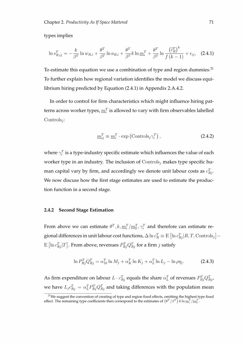
Chapter 2. Productivity As If Space Mattered 71
types implies
ln sTR,ij = − k
βTlnwR,i +
θT
βTln aR,i +
θT
βTk lnmT
i +θT
βTln
(cTR)k
f (k − 1)+ εij, (2.4.1)
To estimate this equation we use a combination of type and region dummies.21
To further explain how regional variation identifies the model we discuss equi-
librium hiring predicted by Equation (2.4.1) in Appendix 2.A.4.2.
In order to control for firm characteristics which might influence hiring pat-
terns across worker types, mTi is allowed to vary with firm observables labelled
Controlsj :
mTij ≡ mT
i · exp(Controlsjγ
Ti
), (2.4.2)
where γTi is a type-industry specific estimate which influences the value of each
worker type in an industry. The inclusion of Controlsj makes type specific hu-
man capital vary by firm, and accordingly we denote unit labour costs as cTRj .
We now discuss how the first stage estimates are used to estimate the produc-
tion function in a second stage.
2.4.2 Second Stage Estimation
From above we can estimate θT , k,mTi /m
TS , γ
Ti and therefore can estimate re-
gional differences in unit labour cost functions, ∆ ln cTR ≡ E[ln cTRj|R, T,Controlsj
]−
E[ln cTRj|T
]. From above, revenues P T
RjQTRj for a firm j satisfy
lnP TRjQ
TRj = αTM lnMj + αTK lnKj + αTL lnLj − ln ρηj. (2.4.3)
As firm expenditure on labour L · cTRj equals the share αTL of revenues P TRjQ
TRj ,
we have LjcTRj = αTLPTRjQ
TRj and taking differences with the population mean
21We suggest the convention of creating of type and region fixed effects, omitting the highest type fixedeffect. The remaining type coefficients then correspond to the estimates of
(θT /βT
)k lnmT
i /mTS .
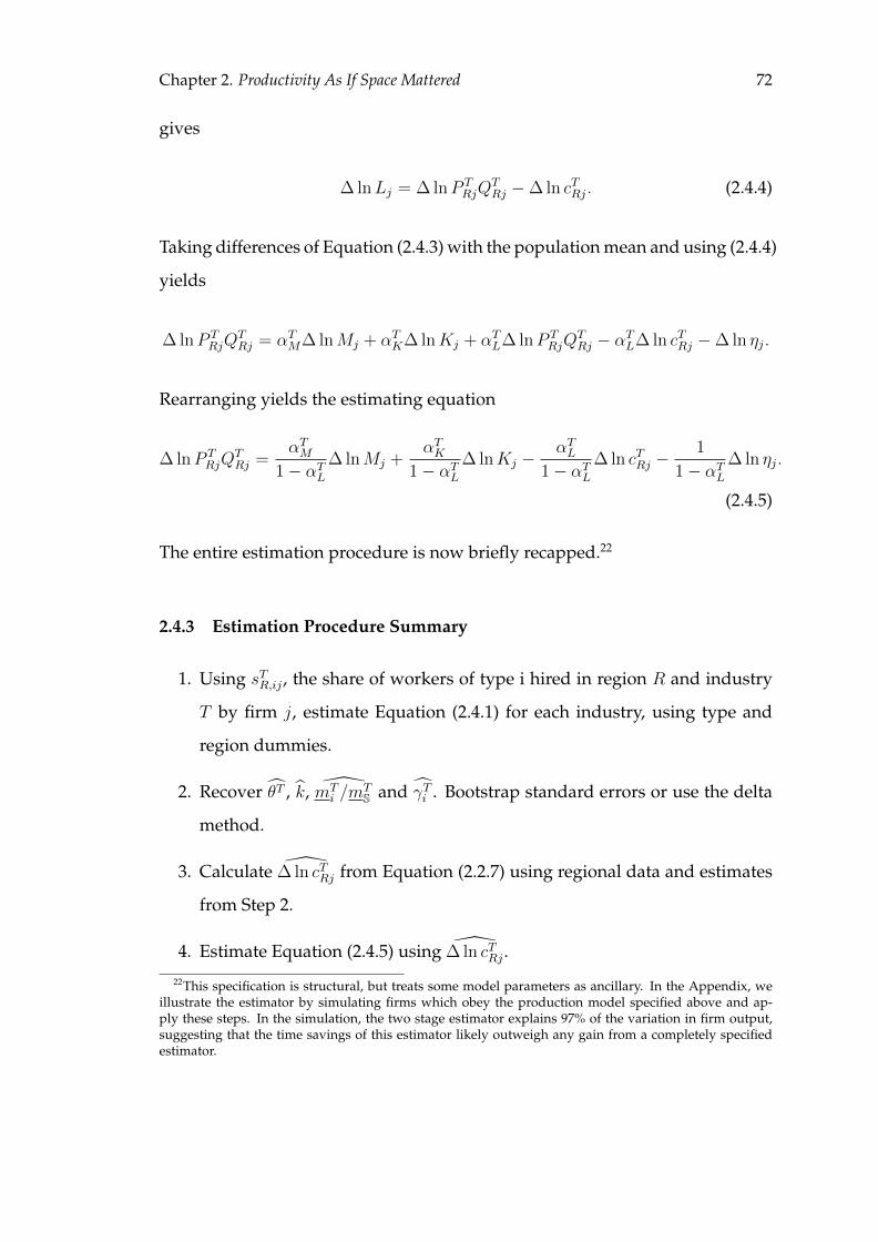
Chapter 2. Productivity As If Space Mattered 72
gives
∆ lnLj = ∆ lnP TRjQ
TRj −∆ ln cTRj. (2.4.4)
Taking differences of Equation (2.4.3) with the population mean and using (2.4.4)
yields
∆ lnP TRjQ
TRj = αTM∆ lnMj + αTK∆ lnKj + αTL∆ lnP T
RjQTRj − αTL∆ ln cTRj −∆ ln ηj.
Rearranging yields the estimating equation
∆ lnP TRjQ
TRj =
αTM1− αTL
∆ lnMj +αTK
1− αTL∆ lnKj −
αTL1− αTL
∆ ln cTRj −1
1− αTL∆ ln ηj.
(2.4.5)
The entire estimation procedure is now briefly recapped.22
2.4.3 Estimation Procedure Summary
1. Using sTR,ij , the share of workers of type i hired in region R and industry
T by firm j, estimate Equation (2.4.1) for each industry, using type and
region dummies.
2. Recover θT , k, mTi /m
TS and γTi . Bootstrap standard errors or use the delta
method.
3. Calculate ∆ ln cTRj from Equation (2.2.7) using regional data and estimates
from Step 2.
4. Estimate Equation (2.4.5) using ∆ ln cTRj .
22This specification is structural, but treats some model parameters as ancillary. In the Appendix, weillustrate the estimator by simulating firms which obey the production model specified above and ap-ply these steps. In the simulation, the two stage estimator explains 97% of the variation in firm output,suggesting that the time savings of this estimator likely outweigh any gain from a completely specifiedestimator.
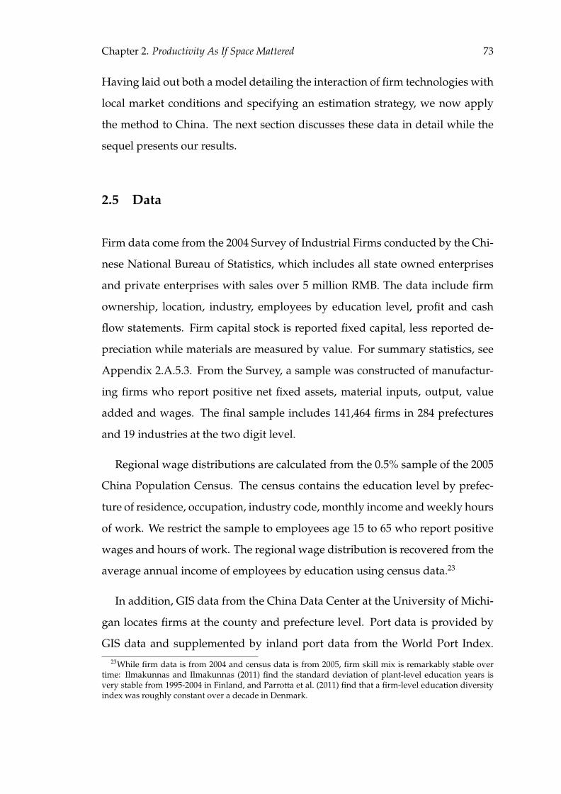
Chapter 2. Productivity As If Space Mattered 73
Having laid out both a model detailing the interaction of firm technologies with
local market conditions and specifying an estimation strategy, we now apply
the method to China. The next section discusses these data in detail while the
sequel presents our results.
2.5 Data
Firm data come from the 2004 Survey of Industrial Firms conducted by the Chi-
nese National Bureau of Statistics, which includes all state owned enterprises
and private enterprises with sales over 5 million RMB. The data include firm
ownership, location, industry, employees by education level, profit and cash
flow statements. Firm capital stock is reported fixed capital, less reported de-
preciation while materials are measured by value. For summary statistics, see
Appendix 2.A.5.3. From the Survey, a sample was constructed of manufactur-
ing firms who report positive net fixed assets, material inputs, output, value
added and wages. The final sample includes 141,464 firms in 284 prefectures
and 19 industries at the two digit level.
Regional wage distributions are calculated from the 0.5% sample of the 2005
China Population Census. The census contains the education level by prefec-
ture of residence, occupation, industry code, monthly income and weekly hours
of work. We restrict the sample to employees age 15 to 65 who report positive
wages and hours of work. The regional wage distribution is recovered from the
average annual income of employees by education using census data.23
In addition, GIS data from the China Data Center at the University of Michi-
gan locates firms at the county and prefecture level. Port data is provided by
GIS data and supplemented by inland port data from the World Port Index.23While firm data is from 2004 and census data is from 2005, firm skill mix is remarkably stable over
time: Ilmakunnas and Ilmakunnas (2011) find the standard deviation of plant-level education years isvery stable from 1995-2004 in Finland, and Parrotta et al. (2011) find that a firm-level education diversityindex was roughly constant over a decade in Denmark.
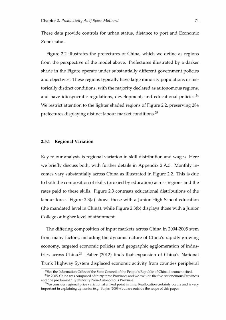
Chapter 2. Productivity As If Space Mattered 74
These data provide controls for urban status, distance to port and Economic
Zone status.
Figure 2.2 illustrates the prefectures of China, which we define as regions
from the perspective of the model above. Prefectures illustrated by a darker
shade in the Figure operate under substantially different government policies
and objectives. These regions typically have large minority populations or his-
torically distinct conditions, with the majority declared as autonomous regions,
and have idiosyncratic regulations, development, and educational policies.24
We restrict attention to the lighter shaded regions of Figure 2.2, preserving 284
prefectures displaying distinct labour market conditions.25
2.5.1 Regional Variation
Key to our analysis is regional variation in skill distribution and wages. Here
we briefly discuss both, with further details in Appendix 2.A.5. Monthly in-
comes vary substantially across China as illustrated in Figure 2.2. This is due
to both the composition of skills (proxied by education) across regions and the
rates paid to these skills. Figure 2.3 contrasts educational distributions of the
labour force. Figure 2.3(a) shows those with a Junior High School education
(the mandated level in China), while Figure 2.3(b) displays those with a Junior
College or higher level of attainment.
The differing composition of input markets across China in 2004-2005 stem
from many factors, including the dynamic nature of China’s rapidly growing
economy, targeted economic policies and geographic agglomeration of indus-
tries across China.26 Faber (2012) finds that expansion of China’s National
Trunk Highway System displaced economic activity from counties peripheral24See the Information Office of the State Council of the People’s Republic of China document cited.25In 2005, China was composed of thirty three Provinces and we exclude the five Autonomous Provinces
and one predominantly minority Non-Autonomous Province.26We consider regional price variation at a fixed point in time. Reallocation certainly occurs and is very
important in explaining dynamics (e.g. Borjas (2003)) but are outside the scope of this paper.
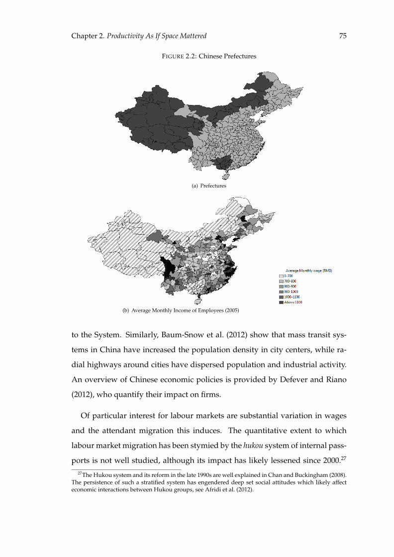
Chapter 2. Productivity As If Space Mattered 75
FIGURE 2.2: Chinese Prefectures
(a) Prefectures
(b) Average Monthly Income of Employees (2005)
to the System. Similarly, Baum-Snow et al. (2012) show that mass transit sys-
tems in China have increased the population density in city centers, while ra-
dial highways around cities have dispersed population and industrial activity.
An overview of Chinese economic policies is provided by Defever and Riano
(2012), who quantify their impact on firms.
Of particular interest for labour markets are substantial variation in wages
and the attendant migration this induces. The quantitative extent to which
labour market migration has been stymied by the hukou system of internal pass-
ports is not well studied, although its impact has likely lessened since 2000.27
27The Hukou system and its reform in the late 1990s are well explained in Chan and Buckingham (2008).The persistence of such a stratified system has engendered deep set social attitudes which likely affecteconomic interactions between Hukou groups, see Afridi et al. (2012).
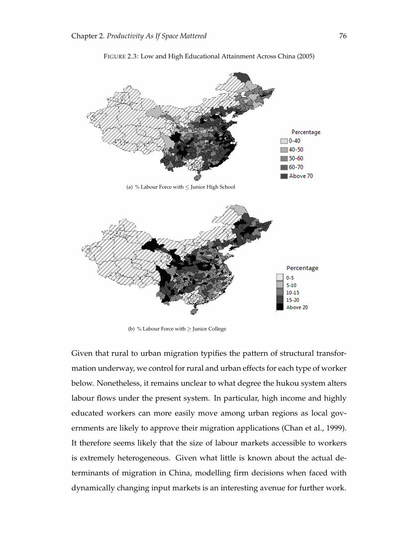
Chapter 2. Productivity As If Space Mattered 76
FIGURE 2.3: Low and High Educational Attainment Across China (2005)
(a) % Labour Force with ≤ Junior High School
(b) % Labour Force with ≥ Junior College
Given that rural to urban migration typifies the pattern of structural transfor-
mation underway, we control for rural and urban effects for each type of worker
below. Nonetheless, it remains unclear to what degree the hukou system alters
labour flows under the present system. In particular, high income and highly
educated workers can more easily move among urban regions as local gov-
ernments are likely to approve their migration applications (Chan et al., 1999).
It therefore seems likely that the size of labour markets accessible to workers
is extremely heterogeneous. Given what little is known about the actual de-
terminants of migration in China, modelling firm decisions when faced with
dynamically changing input markets is an interesting avenue for further work.

Chapter 2. Productivity As If Space Mattered 77
2.5.2 Worker Types
Our definition of workers is people between ages 15 and 65 who work outside
the agricultural sector and are not employers, self-employed, or in a family
business. Our definition of distinct, imperfectly substitutable worker types is
based primarily on formal schooling attained. Census data from 2005 shows
that the average years of schooling for workers in China ranges from 8.5 to 11.8
years across provinces, with sparse postgraduate education. The most common
level of formal education is at the Junior High School level or below. Reflecting
substantial wage differences by gender within that group, we define Type 1
workers as Junior High School or Below: Female and Type 2 workers as Junior
High School or Below: Male.28 Completion of Senior High School defines Type
3 and completion of Junior College or higher education defines Type 4.
Having discussed the data, we now apply the estimation procedure devel-
oped above.
2.6 Estimation Results
This section reports our estimation results, then turns to a discussion of the
quantitative labour cost and productivity differences accounted for by local
market conditions in China. The section continues by testing the firm loca-
tion implications of the model, finding broad support that economic activity
locates where estimated unit labour costs are lower. Finally, we compare esti-
mation results of our unit cost based method with one approach common in the
literature, which assumes that labour types are perfectly substitutable.28Differentiation of gender for low skill labour is especially important in developing countries as a
variety of influences result in imperfect substitutability across gender. Bernhofen and Brown (2011) dis-tinguish between skilled male labour, unskilled male labour and female labour and find that the factorprices across these types differ substantially.
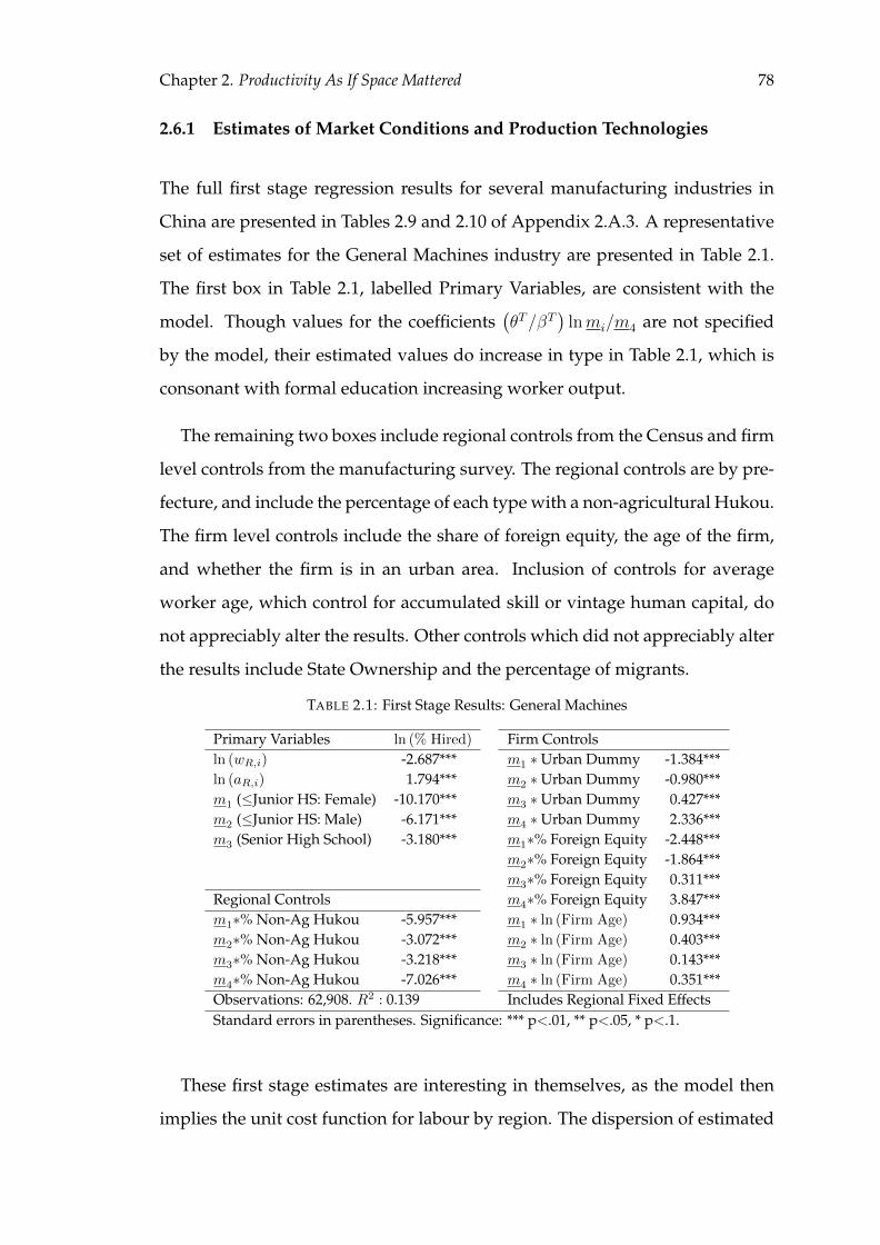
Chapter 2. Productivity As If Space Mattered 78
2.6.1 Estimates of Market Conditions and Production Technologies
The full first stage regression results for several manufacturing industries in
China are presented in Tables 2.9 and 2.10 of Appendix 2.A.3. A representative
set of estimates for the General Machines industry are presented in Table 2.1.
The first box in Table 2.1, labelled Primary Variables, are consistent with the
model. Though values for the coefficients(θT/βT
)lnmi/m4 are not specified
by the model, their estimated values do increase in type in Table 2.1, which is
consonant with formal education increasing worker output.
The remaining two boxes include regional controls from the Census and firm
level controls from the manufacturing survey. The regional controls are by pre-
fecture, and include the percentage of each type with a non-agricultural Hukou.
The firm level controls include the share of foreign equity, the age of the firm,
and whether the firm is in an urban area. Inclusion of controls for average
worker age, which control for accumulated skill or vintage human capital, do
not appreciably alter the results. Other controls which did not appreciably alter
the results include State Ownership and the percentage of migrants.
TABLE 2.1: First Stage Results: General Machines
Primary Variables ln (% Hired) Firm Controlsln (wR,i) -2.687*** m1 ∗Urban Dummy -1.384***ln (aR,i) 1.794*** m2 ∗Urban Dummy -0.980***m1 (≤Junior HS: Female) -10.170*** m3 ∗Urban Dummy 0.427***m2 (≤Junior HS: Male) -6.171*** m4 ∗Urban Dummy 2.336***m3 (Senior High School) -3.180*** m1∗% Foreign Equity -2.448***
m2∗% Foreign Equity -1.864***m3∗% Foreign Equity 0.311***
Regional Controls m4∗% Foreign Equity 3.847***m1∗% Non-Ag Hukou -5.957*** m1 ∗ ln (Firm Age) 0.934***m2∗% Non-Ag Hukou -3.072*** m2 ∗ ln (Firm Age) 0.403***m3∗% Non-Ag Hukou -3.218*** m3 ∗ ln (Firm Age) 0.143***m4∗% Non-Ag Hukou -7.026*** m4 ∗ ln (Firm Age) 0.351***Observations: 62,908. R2 : 0.139 Includes Regional Fixed EffectsStandard errors in parentheses. Significance: *** p<.01, ** p<.05, * p<.1.
These first stage estimates are interesting in themselves, as the model then
implies the unit cost function for labour by region. The dispersion of estimated
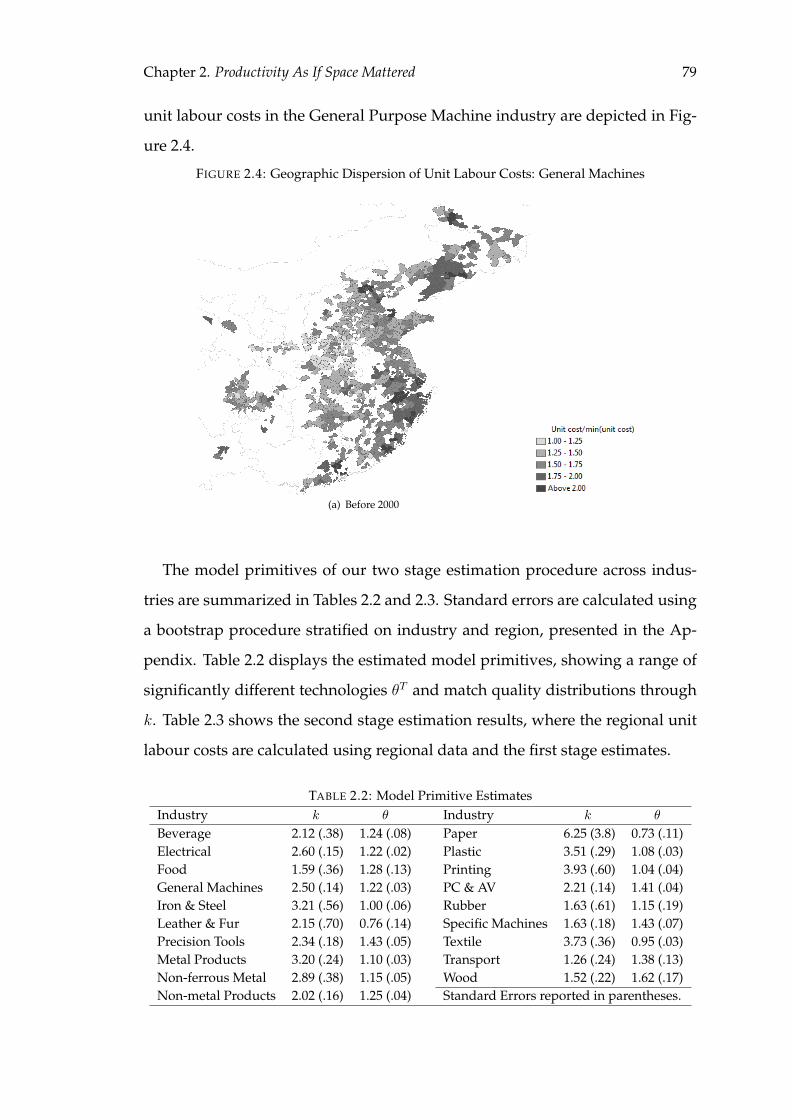
Chapter 2. Productivity As If Space Mattered 79
unit labour costs in the General Purpose Machine industry are depicted in Fig-
ure 2.4.
FIGURE 2.4: Geographic Dispersion of Unit Labour Costs: General Machines
(a) Before 2000
The model primitives of our two stage estimation procedure across indus-
tries are summarized in Tables 2.2 and 2.3. Standard errors are calculated using
a bootstrap procedure stratified on industry and region, presented in the Ap-
pendix. Table 2.2 displays the estimated model primitives, showing a range of
significantly different technologies θT and match quality distributions through
k. Table 2.3 shows the second stage estimation results, where the regional unit
labour costs are calculated using regional data and the first stage estimates.
TABLE 2.2: Model Primitive EstimatesIndustry k θ Industry k θ
Beverage 2.12 (.38) 1.24 (.08) Paper 6.25 (3.8) 0.73 (.11)Electrical 2.60 (.15) 1.22 (.02) Plastic 3.51 (.29) 1.08 (.03)Food 1.59 (.36) 1.28 (.13) Printing 3.93 (.60) 1.04 (.04)General Machines 2.50 (.14) 1.22 (.03) PC & AV 2.21 (.14) 1.41 (.04)Iron & Steel 3.21 (.56) 1.00 (.06) Rubber 1.63 (.61) 1.15 (.19)Leather & Fur 2.15 (.70) 0.76 (.14) Specific Machines 1.63 (.18) 1.43 (.07)Precision Tools 2.34 (.18) 1.43 (.05) Textile 3.73 (.36) 0.95 (.03)Metal Products 3.20 (.24) 1.10 (.03) Transport 1.26 (.24) 1.38 (.13)Non-ferrous Metal 2.89 (.38) 1.15 (.05) Wood 1.52 (.22) 1.62 (.17)Non-metal Products 2.02 (.16) 1.25 (.04) Standard Errors reported in parentheses.
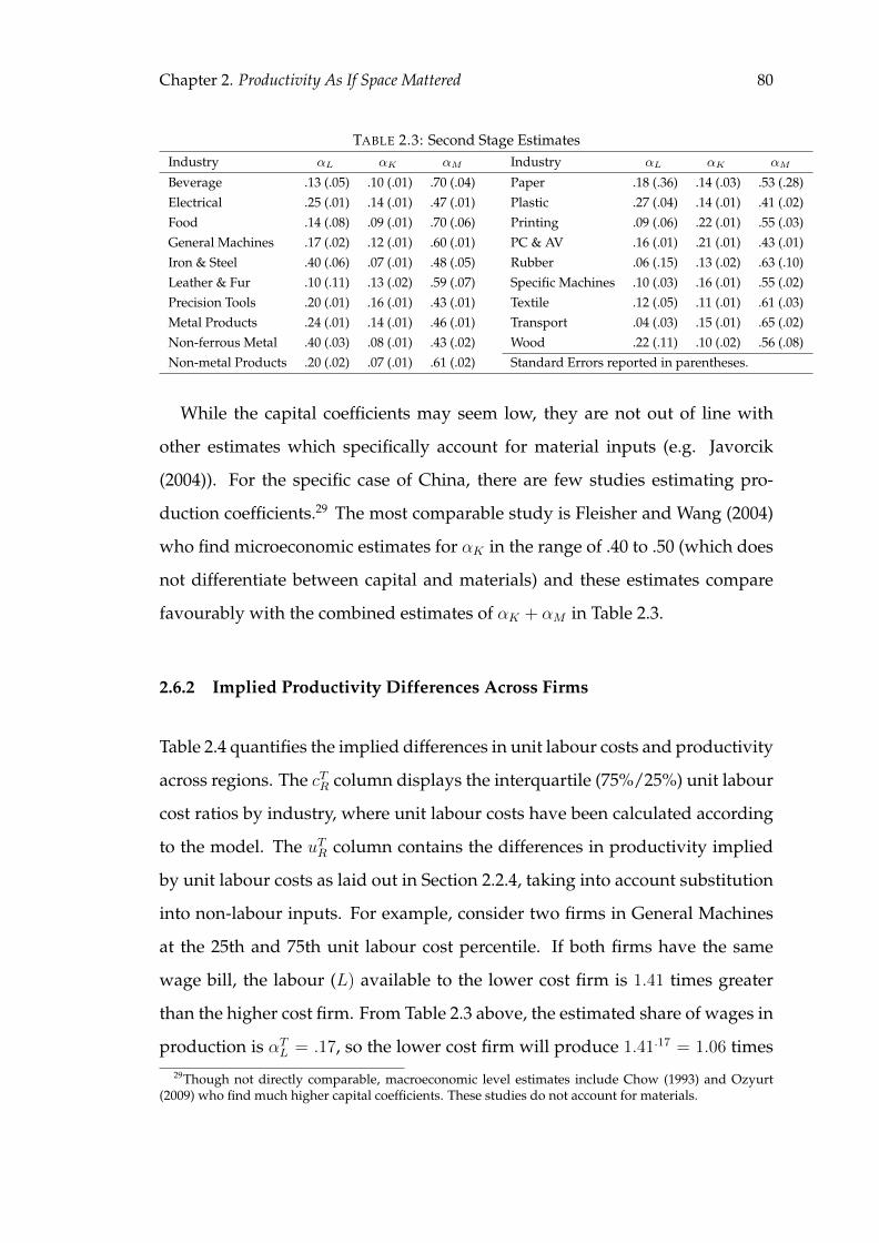
Chapter 2. Productivity As If Space Mattered 80
TABLE 2.3: Second Stage EstimatesIndustry αL αK αM Industry αL αK αM
Beverage .13 (.05) .10 (.01) .70 (.04) Paper .18 (.36) .14 (.03) .53 (.28)Electrical .25 (.01) .14 (.01) .47 (.01) Plastic .27 (.04) .14 (.01) .41 (.02)Food .14 (.08) .09 (.01) .70 (.06) Printing .09 (.06) .22 (.01) .55 (.03)General Machines .17 (.02) .12 (.01) .60 (.01) PC & AV .16 (.01) .21 (.01) .43 (.01)Iron & Steel .40 (.06) .07 (.01) .48 (.05) Rubber .06 (.15) .13 (.02) .63 (.10)Leather & Fur .10 (.11) .13 (.02) .59 (.07) Specific Machines .10 (.03) .16 (.01) .55 (.02)Precision Tools .20 (.01) .16 (.01) .43 (.01) Textile .12 (.05) .11 (.01) .61 (.03)Metal Products .24 (.01) .14 (.01) .46 (.01) Transport .04 (.03) .15 (.01) .65 (.02)Non-ferrous Metal .40 (.03) .08 (.01) .43 (.02) Wood .22 (.11) .10 (.02) .56 (.08)Non-metal Products .20 (.02) .07 (.01) .61 (.02) Standard Errors reported in parentheses.
While the capital coefficients may seem low, they are not out of line with
other estimates which specifically account for material inputs (e.g. Javorcik
(2004)). For the specific case of China, there are few studies estimating pro-
duction coefficients.29 The most comparable study is Fleisher and Wang (2004)
who find microeconomic estimates for αK in the range of .40 to .50 (which does
not differentiate between capital and materials) and these estimates compare
favourably with the combined estimates of αK + αM in Table 2.3.
2.6.2 Implied Productivity Differences Across Firms
Table 2.4 quantifies the implied differences in unit labour costs and productivity
across regions. The cTR column displays the interquartile (75%/25%) unit labour
cost ratios by industry, where unit labour costs have been calculated according
to the model. The uTR column contains the differences in productivity implied
by unit labour costs as laid out in Section 2.2.4, taking into account substitution
into non-labour inputs. For example, consider two firms in General Machines
at the 25th and 75th unit labour cost percentile. If both firms have the same
wage bill, the labour (L) available to the lower cost firm is 1.41 times greater
than the higher cost firm. From Table 2.3 above, the estimated share of wages in
production is αTL = .17, so the lower cost firm will produce 1.41.17 = 1.06 times29Though not directly comparable, macroeconomic level estimates include Chow (1993) and Ozyurt
(2009) who find much higher capital coefficients. These studies do not account for materials.
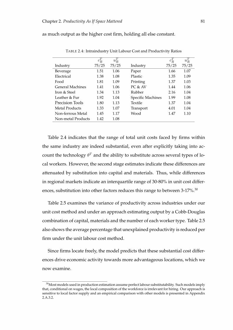
Chapter 2. Productivity As If Space Mattered 81
as much output as the higher cost firm, holding all else constant.
TABLE 2.4: Intraindustry Unit Labour Cost and Productivity Ratios
cTR uTR cTR uTRIndustry 75/25 75/25 Industry 75/25 75/25Beverage 1.51 1.06 Paper 1.66 1.07Electrical 1.38 1.08 Plastic 1.35 1.09Food 1.81 1.09 Printing 1.37 1.03General Machines 1.41 1.06 PC & AV 1.44 1.06Iron & Steel 1.34 1.13 Rubber 2.16 1.04Leather & Fur 1.92 1.04 Specific Machines 1.99 1.08Precision Tools 1.80 1.13 Textile 1.37 1.04Metal Products 1.33 1.07 Transport 4.01 1.04Non-ferrous Metal 1.45 1.17 Wood 1.47 1.10Non-metal Products 1.42 1.08
Table 2.4 indicates that the range of total unit costs faced by firms within
the same industry are indeed substantial, even after explicitly taking into ac-
count the technology θT and the ability to substitute across several types of lo-
cal workers. However, the second stage estimates indicate these differences are
attenuated by substitution into capital and materials. Thus, while differences
in regional markets indicate an interquartile range of 30-80% in unit cost differ-
ences, substitution into other factors reduces this range to between 3-17%.30
Table 2.5 examines the variance of productivity across industries under our
unit cost method and under an approach estimating output by a Cobb-Douglas
combination of capital, materials and the number of each worker type. Table 2.5
also shows the average percentage that unexplained productivity is reduced per
firm under the unit labour cost method.
Since firms locate freely, the model predicts that these substantial cost differ-
ences drive economic activity towards more advantageous locations, which we
now examine.
30Most models used in production estimation assume perfect labour substitutability. Such models implythat, conditional on wages, the local composition of the workforce is irrelevant for hiring. Our approach issensitive to local factor supply and an empirical comparison with other models is presented in Appendix2.A.3.2.
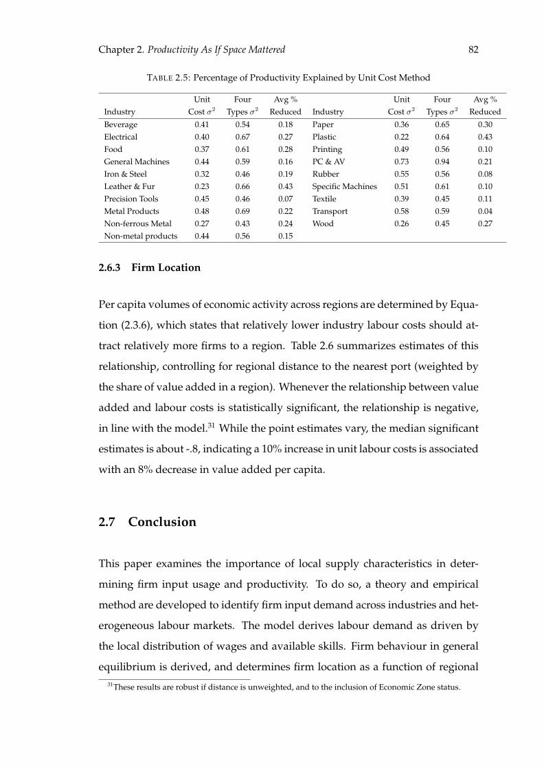
Chapter 2. Productivity As If Space Mattered 82
TABLE 2.5: Percentage of Productivity Explained by Unit Cost Method
Unit Four Avg % Unit Four Avg %Industry Cost σ2 Types σ2 Reduced Industry Cost σ2 Types σ2 Reduced
Beverage 0.41 0.54 0.18 Paper 0.36 0.65 0.30Electrical 0.40 0.67 0.27 Plastic 0.22 0.64 0.43Food 0.37 0.61 0.28 Printing 0.49 0.56 0.10General Machines 0.44 0.59 0.16 PC & AV 0.73 0.94 0.21Iron & Steel 0.32 0.46 0.19 Rubber 0.55 0.56 0.08Leather & Fur 0.23 0.66 0.43 Specific Machines 0.51 0.61 0.10Precision Tools 0.45 0.46 0.07 Textile 0.39 0.45 0.11Metal Products 0.48 0.69 0.22 Transport 0.58 0.59 0.04Non-ferrous Metal 0.27 0.43 0.24 Wood 0.26 0.45 0.27Non-metal products 0.44 0.56 0.15
2.6.3 Firm Location
Per capita volumes of economic activity across regions are determined by Equa-
tion (2.3.6), which states that relatively lower industry labour costs should at-
tract relatively more firms to a region. Table 2.6 summarizes estimates of this
relationship, controlling for regional distance to the nearest port (weighted by
the share of value added in a region). Whenever the relationship between value
added and labour costs is statistically significant, the relationship is negative,
in line with the model.31 While the point estimates vary, the median significant
estimates is about -.8, indicating a 10% increase in unit labour costs is associated
with an 8% decrease in value added per capita.
2.7 Conclusion
This paper examines the importance of local supply characteristics in deter-
mining firm input usage and productivity. To do so, a theory and empirical
method are developed to identify firm input demand across industries and het-
erogeneous labour markets. The model derives labour demand as driven by
the local distribution of wages and available skills. Firm behaviour in general
equilibrium is derived, and determines firm location as a function of regional31These results are robust if distance is unweighted, and to the inclusion of Economic Zone status.
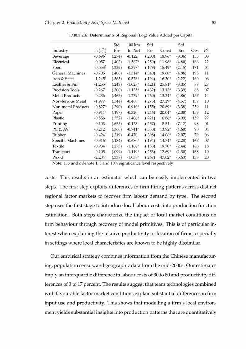
Chapter 2. Productivity As If Space Mattered 83
TABLE 2.6: Determinants of Regional (Log) Value Added per Capita
Std 100 km Std StdIndustry ln
(cTR)
Err to Port Err Const Err Obs R2
Beverage -0.696b (.274) -0.122 (.200) 18.96a (3.36) 155 .03Electrical -0.057 (.403) -1.567a (.259) 11.98b (4.80) 166 .22Food -0.553b (.229) -0.397b (.179) 15.49a (2.15) 171 .04General Machines -0.705c (.400) -1.314a (.340) 19.68a (4.86) 195 .11Iron & Steel -1.245b (.565) -0.576a (.194) 16.30a (2.22) 160 .06Leather & Fur -1.255a (.249) -1.028b (.421) 25.81a (3.05) 89 .27Precision Tools -0.267 (.300) -1.135b (.432) 13.13a (3.39) 68 .07Metal Products -0.236 (.463) -1.239a (.260) 13.24a (4.86) 157 .14Non-ferrous Metal -1.977a (.544) -0.468c (.275) 27.29a (4.57) 139 .10Non-metal Products -0.827a (.290) -0.910a (.155) 20.89a (3.38) 259 .11Paper -0.911a (.197) -0.320 (.246) 20.04a (2.08) 159 .12Plastic -0.556 (.352) -1.406a (.221) 16.86a (3.99) 159 .22Printing 0.103 (.655) -0.123 (.257) 8.54 (7.12) 98 .01PC & AV -0.212 (.366) -0.741b (.333) 13.92a (4.60) 90 .04Rubber -0.424c (.219) -0.470 (.398) 14.06a (2.07) 79 .06Specific Machines -0.316c (.184) -0.680a (.194) 14.74a (2.28) 167 .07Textile -0.934a (.273) -1.168a (.153) 19.70a (2.44) 186 .18Transport -0.105 (.099) -1.119a (.253) 12.69a (1.30) 168 .10Wood -2.234a (.338) -1.038a (.267) 47.02a (5.63) 133 .20Note: a, b and c denote 1, 5 and 10% significance level respectively.
costs. This results in an estimator which can be easily implemented in two
steps. The first step exploits differences in firm hiring patterns across distinct
regional factor markets to recover firm labour demand by type. The second
step uses the first stage to introduce local labour costs into production function
estimation. Both steps characterize the impact of local market conditions on
firm behaviour through recovery of model primitives. This is of particular in-
terest when explaining the relative productivity or location of firms, especially
in settings where local characteristics are known to be highly dissimilar.
Our empirical strategy combines information from the Chinese manufactur-
ing, population census, and geographic data from the mid-2000s. Our estimates
imply an interquartile difference in labour costs of 30 to 80 and productivity dif-
ferences of 3 to 17 percent. The results suggest that team technologies combined
with favourable factor market conditions explain substantial differences in firm
input use and productivity. This shows that modelling a firm’s local environ-
ment yields substantial insights into production patterns that are quantitatively

Chapter 2. Productivity As If Space Mattered 84
important.
The importance of local factor markets for understanding firm behaviour
suggests new dimensions for policy analysis. For instance, regions with labour
markets which generate lower unit labour costs tend to attract higher levels of
firm activity within an industry. As unit labour costs depend not only on the
level of wages, but rather the distribution of wages and worker types that rep-
resent substitution options, this yields a more varied view of how educational
policy or flows of different worker types could impact firms. Taken as a whole,
our results show that policy changes which influence the composition of re-
gional labour markets will have sizable effects on firm behaviour, productivity
and location.
Finally, nothing precludes the application of this paper’s approach beyond
China, and it is suitable for analysing regions which exhibit a high degree of
labour market heterogeneity. As the model affords the interpretation of trade
between countries which have high barriers to immigration but low barriers to
capital and input flows, it is also suitable for analysing firm behaviour across
national borders. Further work could leverage or extend the approach of com-
bining firm, census and geographic data to better understand the role of local
factor markets on firm behaviour.
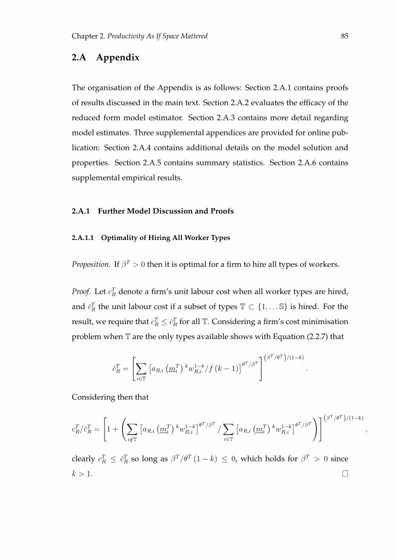
Chapter 2. Productivity As If Space Mattered 85
2.A Appendix
The organisation of the Appendix is as follows: Section 2.A.1 contains proofs
of results discussed in the main text. Section 2.A.2 evaluates the efficacy of the
reduced form model estimator. Section 2.A.3 contains more detail regarding
model estimates. Three supplemental appendices are provided for online pub-
lication: Section 2.A.4 contains additional details on the model solution and
properties. Section 2.A.5 contains summary statistics. Section 2.A.6 contains
supplemental empirical results.
2.A.1 Further Model Discussion and Proofs
2.A.1.1 Optimality of Hiring All Worker Types
Proposition. If βT > 0 then it is optimal for a firm to hire all types of workers.
Proof. Let cTR denote a firm’s unit labour cost when all worker types are hired,
and cTR the unit labour cost if a subset of types T ⊂ {1, . . .S} is hired. For the
result, we require that cTR ≤ cTR for all T. Considering a firm’s cost minimisation
problem when T are the only types available shows with Equation (2.2.7) that
cTR =
[∑i∈T
[aR,i
(mTi
)kw1−k
R,i /f (k − 1)]θT /βT](βT /θT )/(1−k)
.
Considering then that
cTR/cTR =
[1 +
(∑i/∈T
[aR,i
(mTi
)kw1−k
R,i
]θT /βT/∑i∈T
[aR,i
(mTi
)kw1−k
R,i
]θT /βT)](βT /θT )/(1−k)
,
clearly cTR ≤ cTR so long as βT/θT (1− k) ≤ 0, which holds for βT > 0 since
k > 1.
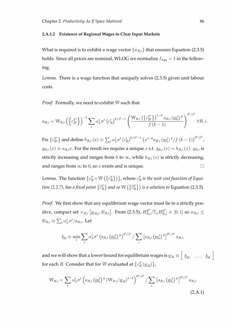
Chapter 2. Productivity As If Space Mattered 86
2.A.1.2 Existence of Regional Wages to Clear Input Markets
What is required is to exhibit a wage vector {wR,i} that ensures Equation (2.3.5)
holds. Since all prices are nominal, WLOG we normalize IAgg = 1 in the follow-
ing.
Lemma. There is a wage function that uniquely solves (2.3.5) given unit labour
costs.
Proof. Formally, we need to exhibit W such that
aR,i = WR,i
({cT′
R′
})−1∑t
αtLσt(ctR)k/βt−1(WR,i
({cT′
R′
})1−kaR,i (m
ti)k
f (k − 1)
)θt/βt
∀R, i.
Fix{cT′
R′
}and define hR,i (x) ≡
∑t α
tLσ
t (ctR)k/βt−1 (
x1−kaR,i (mti)k/f (k − 1)
)θt/βt ,gR,i (x) ≡ aR,ix. For the result we require a unique x s.t. gR,i (x) = hR,i (x). gR,i is
strictly increasing and ranges from 0 to∞, while hR,i (x) is strictly decreasing,
and ranges from∞ to 0, so x exists and is unique.
Lemma. The function{cTR ◦W
({cTR})}
, where cTR is the unit cost function of Equa-
tion (2.2.7), has a fixed point{cTR}
and so W({cTR})
is a solution to Equation (2.3.5).
Proof. We first show that any equilibrium wage vector must lie in a strictly pos-
itive, compact set ×R,i[wR,i, wR,i
]. From (2.3.5), HθT
R,i/ΣjHθT
R,j ∈ [0, 1] so wR,i ≤
wR,i ≡∑
t αtLσ
t/aR,i. Let
bR ≡ mini
∑t
αtLσt(aR,i
(mti
)k)θt/βt
/∑i
[aR,i
(mti
)k]θt/βt
aR,i,
and we will show that a lower bound for equilibrium wages iswR ≡[bR, . . . , bR
]for each R. Consider that for W evaluated at
{cTR (wR)
},
WR,i =∑t
αtLσt(aR,i
(mti
)k (WR,i/wR)1−k
)θt/βt/∑i
[aR,i
(mti
)k]θt/βt
aR,i.
(2.A.1)
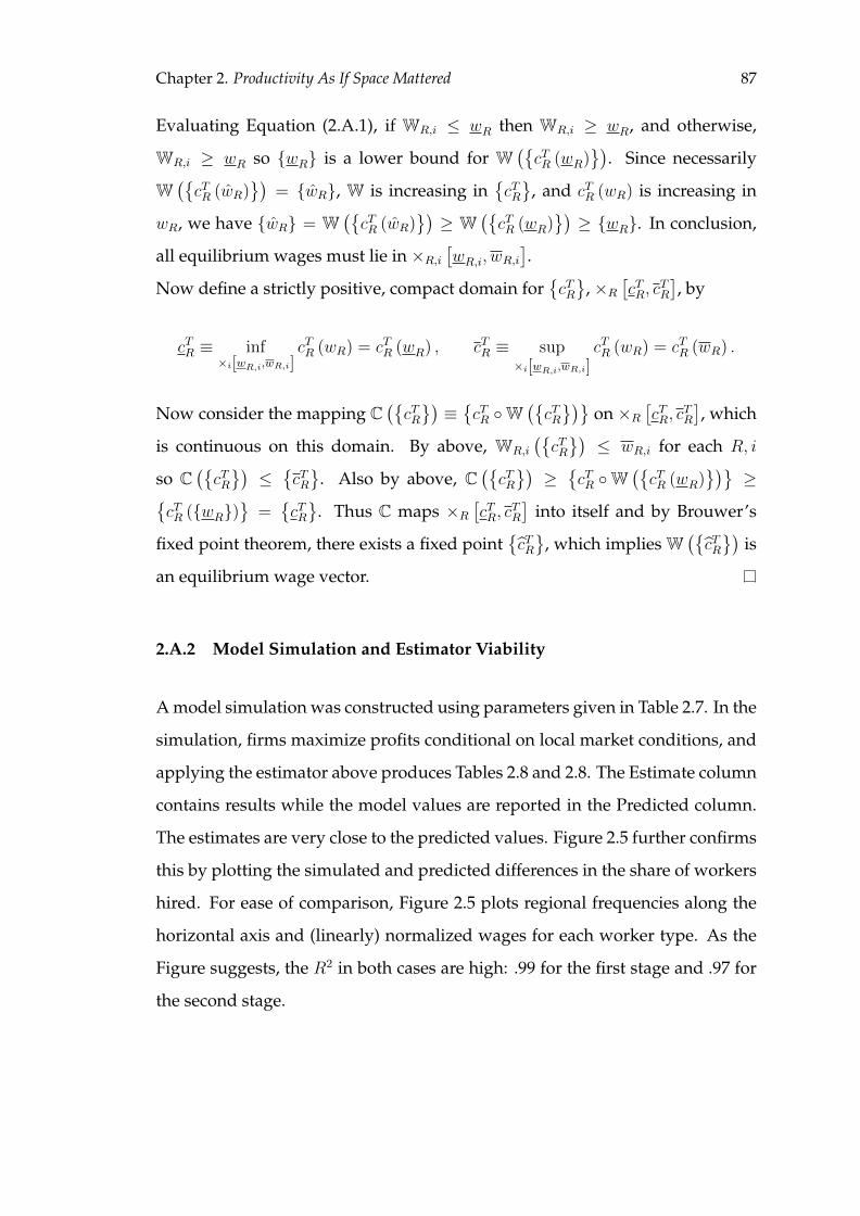
Chapter 2. Productivity As If Space Mattered 87
Evaluating Equation (2.A.1), if WR,i ≤ wR then WR,i ≥ wR, and otherwise,
WR,i ≥ wR so {wR} is a lower bound for W({cTR (wR)
}). Since necessarily
W({cTR (wR)
})= {wR}, W is increasing in
{cTR}
, and cTR (wR) is increasing in
wR, we have {wR} = W({cTR (wR)
})≥ W
({cTR (wR)
})≥ {wR}. In conclusion,
all equilibrium wages must lie in ×R,i[wR,i, wR,i
].
Now define a strictly positive, compact domain for{cTR}
, ×R[cTR, c
TR
], by
cTR ≡ inf×i[wR,i,wR,i]
cTR (wR) = cTR (wR) , cTR ≡ sup×i[wR,i,wR,i]
cTR (wR) = cTR (wR) .
Now consider the mapping C({cTR})≡{cTR ◦W
({cTR})}
on ×R[cTR, c
TR
], which
is continuous on this domain. By above, WR,i
({cTR})≤ wR,i for each R, i
so C({cTR})≤{cTR}
. Also by above, C({cTR})≥{cTR ◦W
({cTR (wR)
})}≥{
cTR ({wR})}
={cTR}
. Thus C maps ×R[cTR, c
TR
]into itself and by Brouwer’s
fixed point theorem, there exists a fixed point{cTR}
, which implies W({cTR})
is
an equilibrium wage vector.
2.A.2 Model Simulation and Estimator Viability
A model simulation was constructed using parameters given in Table 2.7. In the
simulation, firms maximize profits conditional on local market conditions, and
applying the estimator above produces Tables 2.8 and 2.8. The Estimate column
contains results while the model values are reported in the Predicted column.
The estimates are very close to the predicted values. Figure 2.5 further confirms
this by plotting the simulated and predicted differences in the share of workers
hired. For ease of comparison, Figure 2.5 plots regional frequencies along the
horizontal axis and (linearly) normalized wages for each worker type. As the
Figure suggests, the R2 in both cases are high: .99 for the first stage and .97 for
the second stage.
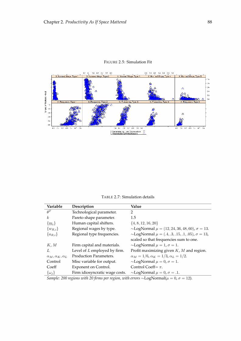
Chapter 2. Productivity As If Space Mattered 88
FIGURE 2.5: Simulation Fit
TABLE 2.7: Simulation details
Variable Description ValueθT Technological parameter. 2k Pareto shape parameter. 1.5{mi} Human capital shifters. {4, 8, 12, 16, 20}{wR,i} Regional wages by type. ∼LogNormal µ = (12, 24, 36, 48, 60), σ = 13.{aR,i} Regional type frequencies. ∼LogNormal µ = (.4, .3, .15, .1, .05), σ = 13,
scaled so that frequencies sum to one.K, M Firm capital and materials. ∼LogNormal µ = 1, σ = 1.L Level of L employed by firm. Profit maximizing given K, M and region.αM , αK , αL Production Parameters. αM = 1/6, αK = 1/3, αL = 1/2.Control Misc variable for output. ∼LogNormal µ = 0, σ = 1.Coeff Exponent on Control. Control Coeff= π.{ωj} Firm idiosyncratic wage costs. ∼LogNormal µ = 0, σ = .1.Sample: 200 regions with 20 firms per region, with errors ∼LogNormal(µ = 0, σ = 12).
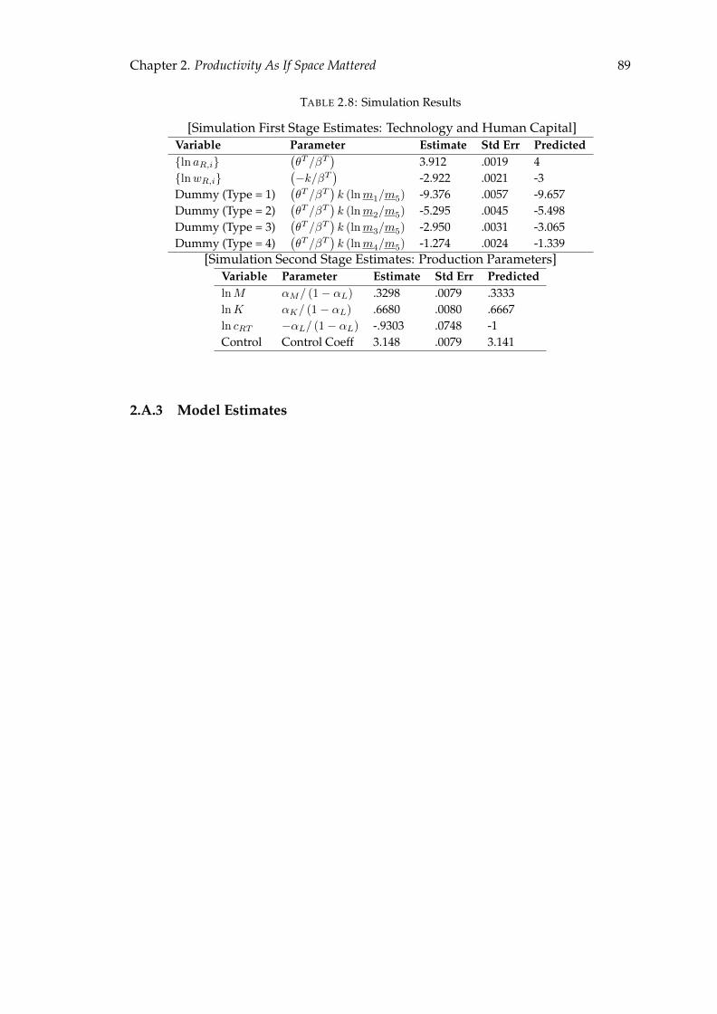
Chapter 2. Productivity As If Space Mattered 89
TABLE 2.8: Simulation Results
[Simulation First Stage Estimates: Technology and Human Capital]Variable Parameter Estimate Std Err Predicted{ln aR,i}
(θT /βT
)3.912 .0019 4
{lnwR,i}(−k/βT
)-2.922 .0021 -3
Dummy (Type = 1)(θT /βT
)k (lnm1/m5) -9.376 .0057 -9.657
Dummy (Type = 2)(θT /βT
)k (lnm2/m5) -5.295 .0045 -5.498
Dummy (Type = 3)(θT /βT
)k (lnm3/m5) -2.950 .0031 -3.065
Dummy (Type = 4)(θT /βT
)k (lnm4/m5) -1.274 .0024 -1.339
[Simulation Second Stage Estimates: Production Parameters]Variable Parameter Estimate Std Err PredictedlnM αM/ (1− αL) .3298 .0079 .3333lnK αK/ (1− αL) .6680 .0080 .6667ln cRT −αL/ (1− αL) -.9303 .0748 -1Control Control Coeff 3.148 .0079 3.141
2.A.3 Model Estimates
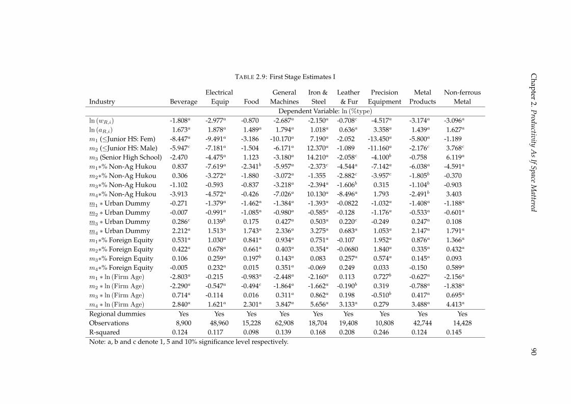
Chapter
2.ProductivityA
sIfSpace
Mattered
90
TABLE 2.9: First Stage Estimates I
Electrical General Iron & Leather Precision Metal Non-ferrousIndustry Beverage Equip Food Machines Steel & Fur Equipment Products Metal
Dependent Variable: ln (%type)
ln (wR,i) -1.808a -2.977a -0.870 -2.687a -2.150a -0.708c -4.517a -3.174a -3.096a
ln (aR,i) 1.673a 1.878a 1.489a 1.794a 1.018a 0.636a 3.358a 1.439a 1.627a
m1 (≤Junior HS: Fem) -8.447a -9.491a -3.186 -10.170a 7.190a -2.052 -13.450a -5.800a -1.189m2 (≤Junior HS: Male) -5.947c -7.181a -1.504 -6.171a 12.370a -1.089 -11.160a -2.176c 3.768c
m3 (Senior High School) -2.470 -4.475a 1.123 -3.180a 14.210a -2.058c -4.100b -0.758 6.119a
m1∗% Non-Ag Hukou 0.837 -7.619a -2.341b -5.957a -2.373c -4.544a -7.142a -6.038a -4.591a
m2∗% Non-Ag Hukou 0.306 -3.272a -1.880 -3.072a -1.355 -2.882c -3.957c -1.805b -0.370m3∗% Non-Ag Hukou -1.102 -0.593 -0.837 -3.218a -2.394a -1.606b 0.315 -1.104b -0.903m4∗% Non-Ag Hukou -3.913 -4.572a -0.426 -7.026a 10.130a -8.496a 1.793 -2.491b 3.403m1 ∗Urban Dummy -0.271 -1.379a -1.462a -1.384a -1.393a -0.0822 -1.032a -1.408a -1.188a
m2 ∗Urban Dummy -0.007 -0.991a -1.085a -0.980a -0.585a -0.128 -1.176a -0.533a -0.601a
m3 ∗Urban Dummy 0.286c 0.139b 0.175 0.427a 0.503a 0.220c -0.249 0.247a 0.108m4 ∗Urban Dummy 2.212a 1.513a 1.743a 2.336a 3.275a 0.683a 1.053a 2.147a 1.791a
m1∗% Foreign Equity 0.531a 1.030a 0.841a 0.934a 0.751a -0.107 1.952a 0.876a 1.366a
m2∗% Foreign Equity 0.422a 0.678a 0.661a 0.403a 0.354a -0.0680 1.840a 0.335a 0.432a
m3∗% Foreign Equity 0.106 0.259a 0.197b 0.143a 0.083 0.257a 0.574a 0.145a 0.093m4∗% Foreign Equity -0.005 0.232a 0.015 0.351a -0.069 0.249 0.033 -0.150 0.589a
m1 ∗ ln (Firm Age) -2.803a -0.215 -0.983a -2.448a -2.160a 0.113 0.727b -0.627a -2.156a
m2 ∗ ln (Firm Age) -2.290a -0.547a -0.494c -1.864a -1.662a -0.190b 0.319 -0.788a -1.838a
m3 ∗ ln (Firm Age) 0.714a -0.114 0.016 0.311a 0.862a 0.198 -0.510b 0.417a 0.695a
m4 ∗ ln (Firm Age) 2.840a 1.621a 2.301a 3.847a 5.656a 3.133a 0.279 3.488a 4.413a
Regional dummies Yes Yes Yes Yes Yes Yes Yes Yes YesObservations 8,900 48,960 15,228 62,908 18,704 19,408 10,808 42,744 14,428R-squared 0.124 0.117 0.098 0.139 0.168 0.208 0.246 0.124 0.145Note: a, b and c denote 1, 5 and 10% significance level respectively.
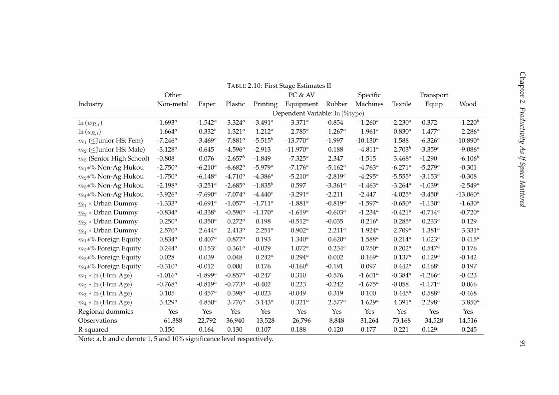
Chapter
2.ProductivityA
sIfSpace
Mattered
91
TABLE 2.10: First Stage Estimates IIOther PC & AV Specific Transport
Industry Non-metal Paper Plastic Printing Equipment Rubber Machines Textile Equip WoodDependent Variable: ln (%type)
ln (wR,i) -1.693a -1.542a -3.324a -3.491a -3.371a -0.854 -1.260a -2.230a -0.372 -1.220b
ln (aR,i) 1.664a 0.332b 1.321a 1.212a 2.785a 1.267a 1.961a 0.830a 1.477a 2.286a
m1 (≤Junior HS: Fem) -7.246a -3.469c -7.881a -5.515b -13.770a -1.997 -10.130a 1.588 -6.326a -10.890a
m2 (≤Junior HS: Male) -3.128a -0.645 -4.596a -2.913 -11.970a 0.188 -4.811a 2.703b -3.359b -9.086a
m3 (Senior High School) -0.808 0.076 -2.657b -1.849 -7.325a 2.347 -1.515 3.468a -1.290 -6.106b
m1∗% Non-Ag Hukou -2.750a -6.210a -6.682a -5.979a -7.176a -5.162a -4.763a -6.271a -5.279a -0.301m2∗% Non-Ag Hukou -1.750a -6.148a -4.710a -4.386a -5.210a -2.819c -4.295a -5.555a -3.153a -0.308m3∗% Non-Ag Hukou -2.198a -3.251a -2.685a -1.835b 0.597 -3.361a -1.463a -3.264a -1.039b -2.549a
m4∗% Non-Ag Hukou -3.926a -7.690a -7.074a -4.440c -3.291a -2.211 -2.447 -4.025a -3.450b -13.060a
m1 ∗Urban Dummy -1.333a -0.691a -1.057a -1.711a -1.881a -0.819a -1.597a -0.650a -1.130a -1.630a
m2 ∗Urban Dummy -0.834a -0.338b -0.590a -1.170a -1.619a -0.603a -1.234a -0.421a -0.714a -0.720a
m3 ∗Urban Dummy 0.250a 0.350a 0.272a 0.198 -0.512a -0.035 0.216b 0.285a 0.233a 0.129m4 ∗Urban Dummy 2.570a 2.644a 2.413a 2.251a 0.902a 2.211a 1.924a 2.709a 1.381a 3.331a
m1∗% Foreign Equity 0.834a 0.407a 0.877a 0.193 1.340a 0.620a 1.588a 0.214a 1.023a 0.415a
m2∗% Foreign Equity 0.244a 0.153c 0.361a -0.029 1.072a 0.234c 0.750a 0.202a 0.547a 0.176m3∗% Foreign Equity 0.028 0.039 0.048 0.242a 0.294a 0.002 0.169a 0.137a 0.129a -0.142m4∗% Foreign Equity -0.310a -0.012 0.000 0.176 -0.160b -0.191 0.097 0.442a 0.168b 0.197m1 ∗ ln (Firm Age) -1.016a -1.899a -0.857a -0.247 0.310 -0.576 -1.601a -0.384a -1.266a -0.423m2 ∗ ln (Firm Age) -0.768a -0.819a -0.773a -0.402 0.223 -0.242 -1.675a -0.058 -1.171a 0.066m3 ∗ ln (Firm Age) 0.105 0.457a 0.398a -0.023 -0.049 0.319 0.100 0.445a 0.588a -0.468m4 ∗ ln (Firm Age) 3.429a 4.850a 3.776a 3.143a 0.321a 2.577a 1.629a 4.391a 2.298a 3.850a
Regional dummies Yes Yes Yes Yes Yes Yes Yes Yes Yes YesObservations 61,388 22,792 36,940 13,528 26,796 8,848 31,264 73,168 34,528 14,516R-squared 0.150 0.164 0.130 0.107 0.188 0.120 0.177 0.221 0.129 0.245Note: a, b and c denote 1, 5 and 10% significance level respectively.
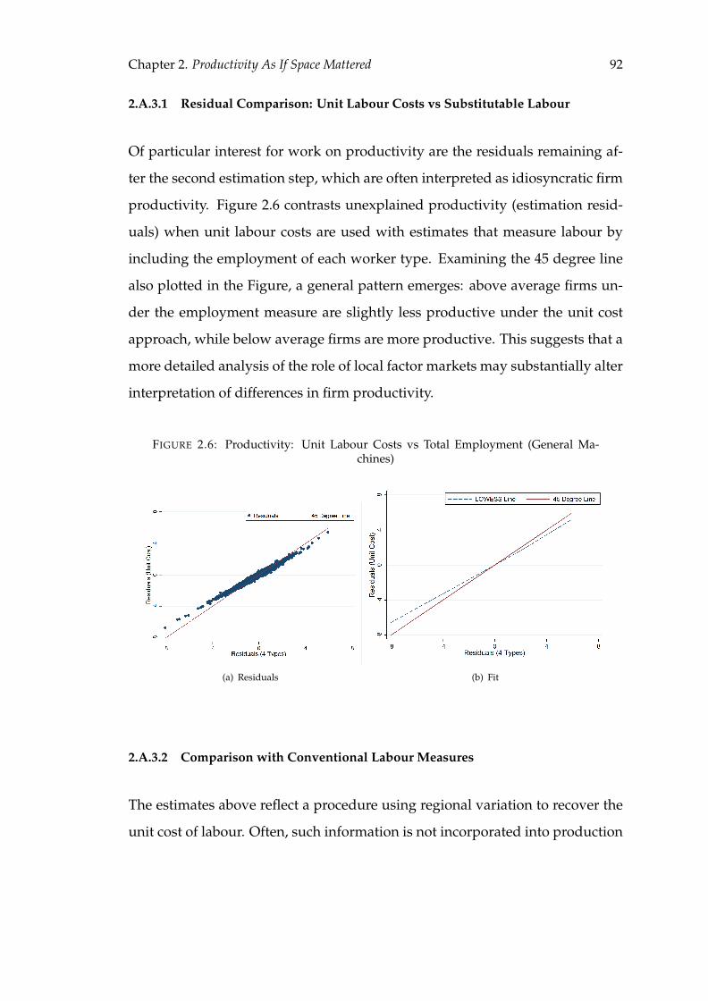
Chapter 2. Productivity As If Space Mattered 92
2.A.3.1 Residual Comparison: Unit Labour Costs vs Substitutable Labour
Of particular interest for work on productivity are the residuals remaining af-
ter the second estimation step, which are often interpreted as idiosyncratic firm
productivity. Figure 2.6 contrasts unexplained productivity (estimation resid-
uals) when unit labour costs are used with estimates that measure labour by
including the employment of each worker type. Examining the 45 degree line
also plotted in the Figure, a general pattern emerges: above average firms un-
der the employment measure are slightly less productive under the unit cost
approach, while below average firms are more productive. This suggests that a
more detailed analysis of the role of local factor markets may substantially alter
interpretation of differences in firm productivity.
FIGURE 2.6: Productivity: Unit Labour Costs vs Total Employment (General Ma-chines)
(a) Residuals (b) Fit
2.A.3.2 Comparison with Conventional Labour Measures
The estimates above reflect a procedure using regional variation to recover the
unit cost of labour. Often, such information is not incorporated into production
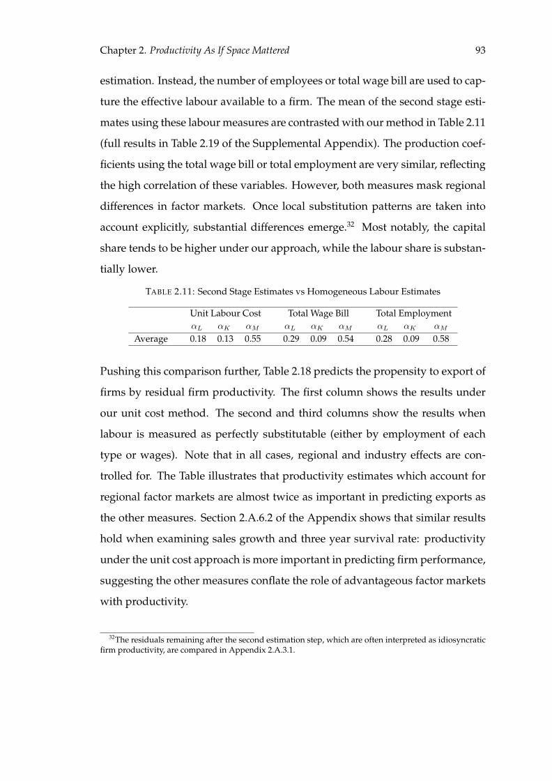
Chapter 2. Productivity As If Space Mattered 93
estimation. Instead, the number of employees or total wage bill are used to cap-
ture the effective labour available to a firm. The mean of the second stage esti-
mates using these labour measures are contrasted with our method in Table 2.11
(full results in Table 2.19 of the Supplemental Appendix). The production coef-
ficients using the total wage bill or total employment are very similar, reflecting
the high correlation of these variables. However, both measures mask regional
differences in factor markets. Once local substitution patterns are taken into
account explicitly, substantial differences emerge.32 Most notably, the capital
share tends to be higher under our approach, while the labour share is substan-
tially lower.
TABLE 2.11: Second Stage Estimates vs Homogeneous Labour Estimates
Unit Labour Cost Total Wage Bill Total EmploymentαL αK αM αL αK αM αL αK αM
Average 0.18 0.13 0.55 0.29 0.09 0.54 0.28 0.09 0.58
Pushing this comparison further, Table 2.18 predicts the propensity to export of
firms by residual firm productivity. The first column shows the results under
our unit cost method. The second and third columns show the results when
labour is measured as perfectly substitutable (either by employment of each
type or wages). Note that in all cases, regional and industry effects are con-
trolled for. The Table illustrates that productivity estimates which account for
regional factor markets are almost twice as important in predicting exports as
the other measures. Section 2.A.6.2 of the Appendix shows that similar results
hold when examining sales growth and three year survival rate: productivity
under the unit cost approach is more important in predicting firm performance,
suggesting the other measures conflate the role of advantageous factor markets
with productivity.
32The residuals remaining after the second estimation step, which are often interpreted as idiosyncraticfirm productivity, are compared in Appendix 2.A.3.1.
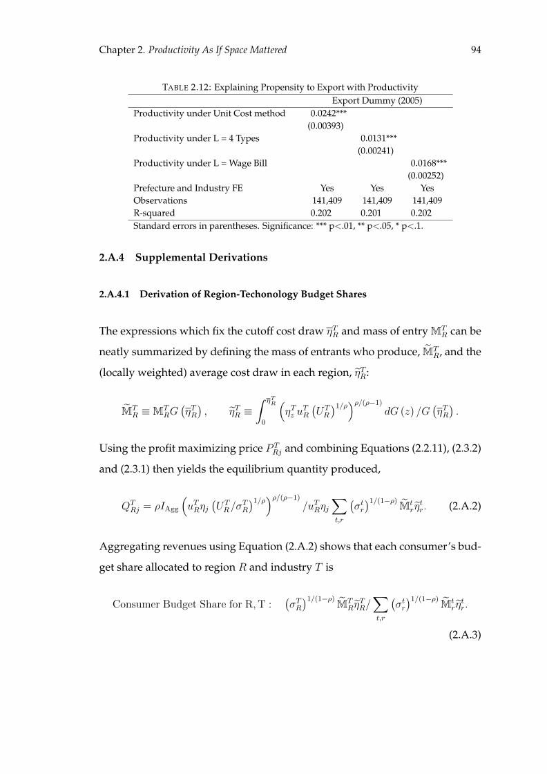
Chapter 2. Productivity As If Space Mattered 94
TABLE 2.12: Explaining Propensity to Export with ProductivityExport Dummy (2005)
Productivity under Unit Cost method 0.0242***(0.00393)
Productivity under L = 4 Types 0.0131***(0.00241)
Productivity under L = Wage Bill 0.0168***(0.00252)
Prefecture and Industry FE Yes Yes YesObservations 141,409 141,409 141,409R-squared 0.202 0.201 0.202Standard errors in parentheses. Significance: *** p<.01, ** p<.05, * p<.1.
2.A.4 Supplemental Derivations
2.A.4.1 Derivation of Region-Techonology Budget Shares
The expressions which fix the cutoff cost draw ηTR and mass of entry MTR can be
neatly summarized by defining the mass of entrants who produce, MTR, and the
(locally weighted) average cost draw in each region, ηTR:
MTR ≡MT
RG(ηTR), ηTR ≡
∫ ηTR
0
(ηTz u
TR
(UTR
)1/ρ)ρ/(ρ−1)dG (z) /G
(ηTR).
Using the profit maximizing price P TRj and combining Equations (2.2.11), (2.3.2)
and (2.3.1) then yields the equilibrium quantity produced,
QTRj = ρIAgg
(uTRηj
(UTR/σ
TR
)1/ρ)ρ/(ρ−1)/uTRηj
∑t,r
(σtr)1/(1−ρ) Mt
rηtr. (2.A.2)
Aggregating revenues using Equation (2.A.2) shows that each consumer’s bud-
get share allocated to region R and industry T is
Consumer Budget Share for R,T :(σTR)1/(1−ρ) MT
RηTR/∑t,r
(σtr)1/(1−ρ) Mt
rηtr.
(2.A.3)
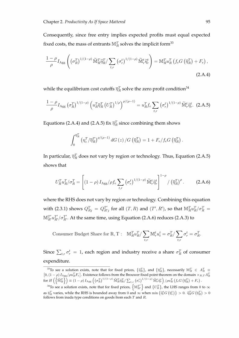
Chapter 2. Productivity As If Space Mattered 95
Consequently, since free entry implies expected profits must equal expected
fixed costs, the mass of entrants MTR solves the implicit form33
1− ρρ
IAgg
((σTR)1/(1−ρ) MT
RηTR/∑t,r
(σtr)1/(1−ρ) Mt
rηtr
)= MT
RuTR
(feG
(ηTR)
+ Fe),
(2.A.4)
while the equilibrium cost cutoffs ηTR solve the zero profit condition34
1− ρρ
IAgg
(σTR)1/(1−ρ) (
uTRηTR
(UTR
)1/ρ)ρ/(ρ−1)= uTRfe
∑t,r
(σtr)1/(1−ρ) Mt
rηtr. (2.A.5)
Equations (2.A.4) and (2.A.5) fix ηTR since combining them shows
∫ ηTR
0
(ηTz /η
TR
)ρ/(ρ−1)dG (z) /G
(ηTR)
= 1 + Fe/feG(ηTR).
In particular, ηTR does not vary by region or technology. Thus, Equation (2.A.5)
shows that
UTRu
TR/σ
TR =
[(1− ρ) IAgg/ρfe
∑t,r
(σtr)1/(1−ρ) Mt
rηtr
]1−ρ/(ηTR)ρ. (2.A.6)
where the RHS does not vary by region or technology. Combining this equation
with (2.3.1) shows QTRj = QT ′
R′j for all (T,R) and (T ′, R′), so that MTRu
TR/σ
TR =
MT ′
R′uT ′
R′/σT ′
R′ . At the same time, using Equation (2.A.6) reduces (2.A.3) to
Consumer Budget Share for R,T : MTRu
TR/∑t,r
Mtru
tt = σTR/
∑t,r
σtr = σTR.
Since∑
t,r σtr = 1, each region and industry receive a share σTR of consumer
expenditure.33To see a solution exists, note that for fixed prices,
{ηTR}
, and{ηTR}
, necessarily MTR ∈ ATR ≡[
0, (1− ρ) IAgg/ρuTRFe
]. Existence follows from the Brouwer fixed point theorem on the domain ×R,TATR
for H({
MTR
})≡ (1− ρ) IAgg
((σTR)1/(1−ρ) MT
RηTR/∑t,r
(σtr)1/(1−ρ) Mt
r ηtr
)/ρuTR
(feG
(ηTR)
+ Fe).
34To see a solution exists, note that for fixed prices,{MT ′
R′
}and
{UTR}
, the LHS ranges from 0 to ∞as ηTR varies, while the RHS is bounded away from 0 and∞ when min
{ηtrG
(ηtr)}
> 0. ηTRG(ηTR)> 0
follows from inada type conditions on goods from each T and R.
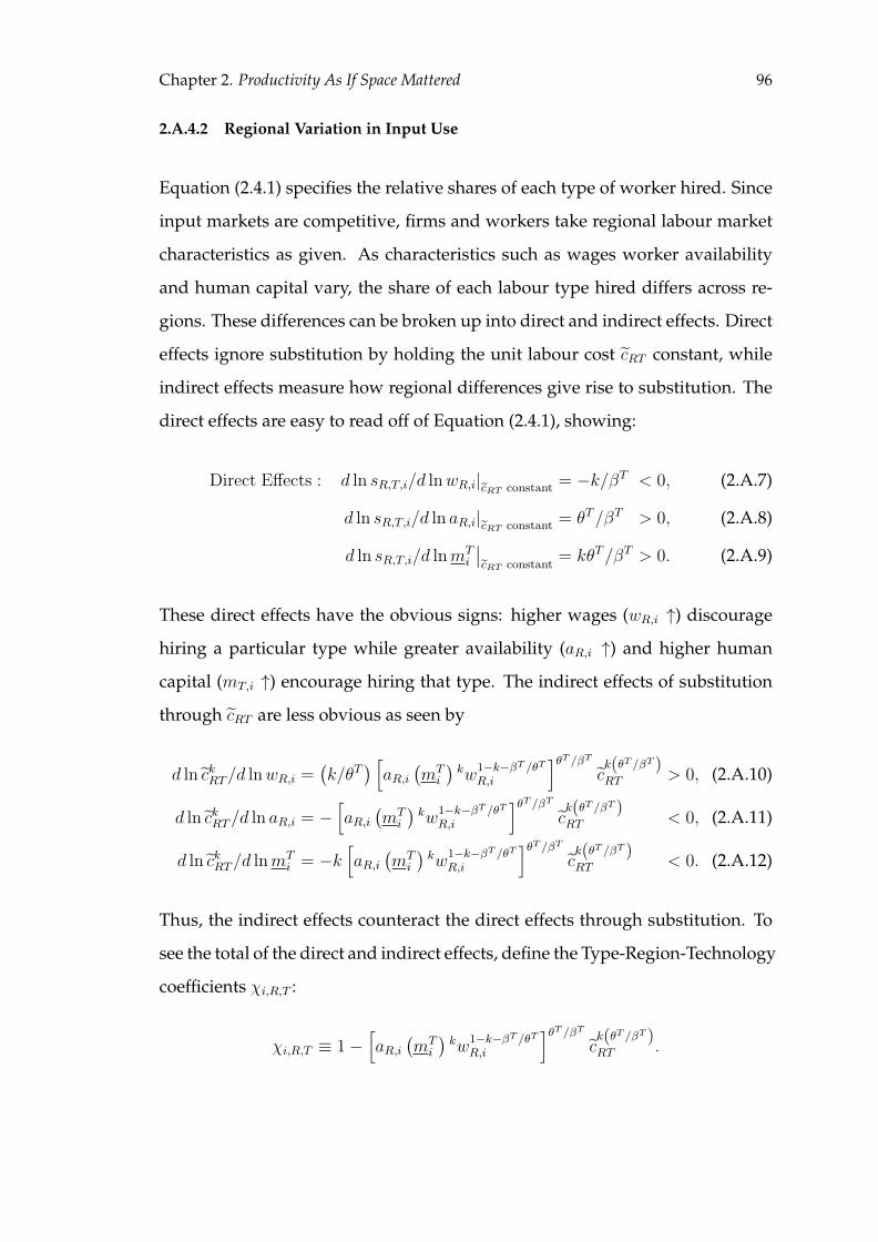
Chapter 2. Productivity As If Space Mattered 96
2.A.4.2 Regional Variation in Input Use
Equation (2.4.1) specifies the relative shares of each type of worker hired. Since
input markets are competitive, firms and workers take regional labour market
characteristics as given. As characteristics such as wages worker availability
and human capital vary, the share of each labour type hired differs across re-
gions. These differences can be broken up into direct and indirect effects. Direct
effects ignore substitution by holding the unit labour cost cRT constant, while
indirect effects measure how regional differences give rise to substitution. The
direct effects are easy to read off of Equation (2.4.1), showing:
Direct Effects : d ln sR,T,i/d lnwR,i|cRT constant = −k/βT < 0, (2.A.7)
d ln sR,T,i/d ln aR,i|cRT constant = θT/βT > 0, (2.A.8)
d ln sR,T,i/d lnmTi
∣∣cRT constant
= kθT/βT > 0. (2.A.9)
These direct effects have the obvious signs: higher wages (wR,i ↑) discourage
hiring a particular type while greater availability (aR,i ↑) and higher human
capital (mT,i ↑) encourage hiring that type. The indirect effects of substitution
through cRT are less obvious as seen by
d ln ckRT/d lnwR,i =(k/θT
) [aR,i
(mTi
)kw
1−k−βT /θTR,i
]θT /βTck(θT /βT )RT > 0, (2.A.10)
d ln ckRT/d ln aR,i = −[aR,i
(mTi
)kw
1−k−βT /θTR,i
]θT /βTck(θT /βT )RT < 0, (2.A.11)
d ln ckRT/d lnmTi = −k
[aR,i
(mTi
)kw
1−k−βT /θTR,i
]θT /βTck(θT /βT )RT < 0. (2.A.12)
Thus, the indirect effects counteract the direct effects through substitution. To
see the total of the direct and indirect effects, define the Type-Region-Technology
coefficients χi,R,T :
χi,R,T ≡ 1−[aR,i
(mTi
)kw
1−k−βT /θTR,i
]θT /βTck(θT /βT )RT .
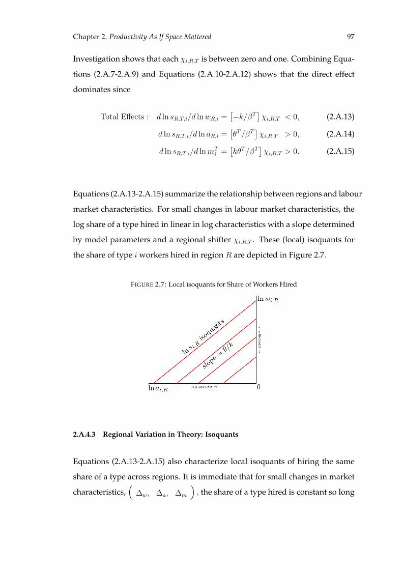
Chapter 2. Productivity As If Space Mattered 97
Investigation shows that each χi,R,T is between zero and one. Combining Equa-
tions (2.A.7-2.A.9) and Equations (2.A.10-2.A.12) shows that the direct effect
dominates since
Total Effects : d ln sR,T,i/d lnwR,i =[−k/βT
]χi,R,T < 0, (2.A.13)
d ln sR,T,i/d ln aR,i =[θT/βT
]χi,R,T > 0, (2.A.14)
d ln sR,T,i/d lnmTi =
[kθT/βT
]χi,R,T > 0. (2.A.15)
Equations (2.A.13-2.A.15) summarize the relationship between regions and labour
market characteristics. For small changes in labour market characteristics, the
log share of a type hired in linear in log characteristics with a slope determined
by model parameters and a regional shifter χi,R,T . These (local) isoquants for
the share of type i workers hired in region R are depicted in Figure 2.7.
FIGURE 2.7: Local isoquants for Share of Workers Hired
2.A.4.3 Regional Variation in Theory: Isoquants
Equations (2.A.13-2.A.15) also characterize local isoquants of hiring the same
share of a type across regions. It is immediate that for small changes in market
characteristics,(
∆w, ∆a, ∆m
), the share of a type hired is constant so long
Chapter 2. Productivity As If Space Mattered 98
as
−(k/θT
)∆w/wR,i + ∆a/aR,i + k∆m/m
Ti = 0.
For instance, firms in regions R and R′ will hire the same fraction of type i
workers for small differences in characteristics (∆w,∆a) so long as
∆w/∆a =(θT/k
)wR,i/aR,i. (2.A.16)
By itself, an increase in type i wages ∆w would cause firms to hire a lower share
of type i workers as indicated by the direct effect. However, Equation (2.A.16)
shows that firms would keep the same share of type i workers if the availability
∆a increases concurrently so that Equation (2.A.16) holds.
2.A.4.4 Derivation of Unit Labour Costs
Unit labour costs by definition solve
Unit Labour Costs : cTR ≡ minH
CT (H|aR, wR) subject to L = φ(H, θT
)·HTOT = 1.
Under the parameterisation Ψ (h) = 1− h−k, Equations (2.2.1) become
Hi = aR,ik/ (k − 1) ·mTi h
1−ki ·N. (2.A.17)
From above,wR,iHi/mTi hiCT (H|aR, wR) = HθT
i /∑
j HθT
j , andL = 1 =(∑
j HθT
j
)1/θTso
hi = wR,iH1−θTi /mT
i CT (H|aR, wR) . (2.A.18)
Substitution now yields
Hi = aR,ik/ (k − 1) ·mTi
(wR,iH
1−θTi /mT
i CT (H|aR, wR))1−k
·N. (2.A.19)
Chapter 2. Productivity As If Space Mattered 99
Further reduction and the definition of βT shows that
HβT
i = HθT+k−kθTi = aR,ik/ (k − 1) ·
(mTi
)kw1−k
R,i CT (H|aR, wR)k−1N. (2.A.20)
Again using(∑
j HθT
j
)1/θT= 1 then shows
1 =∑i
[aR,ik/ (k − 1) ·mT
ikw1−k
R,i
(cTR)k−1
N]θT /βT
. (2.A.21)
From the definition of the cost function we have
cTR = N
[∑i
aR,iwR,ih−ki + fcTR
]=∑i
wR,i ((k − 1) /k)Hi/mTi hi +NfcTR.
Therefore from wR,iHi/mTi hiCT (H|aR, wR) = HθT
i it follows
1 =∑i
(k − 1) /k ·HθT
i +Nf = (k − 1) /k +Nf,
and therefore N = 1/fk. Now from Equation (2.A.21) cTR is seen to be Equation
(2.2.7).
2.A.4.5 Derivation of Employment Shares
Combining Equations (2.A.18), (2.A.20) and N = 1/fk shows
hi = a(1−θT )/βTR,i
(mTi
) −θT /βTw1/βT
R,i
(cTR)−1/βT
/ (f (k − 1))(1−θT )/βT . (2.A.22)
Let ATR,i be the number of type i workers hired to make L = 1, exclusive of fixed
search costs. By definition, ATR,i = N |L=1 aR,i (1−Ψ (hi)) = aR,ih−ki /fk. Using
Equation (2.A.22),
ATR,i = k−1 (k − 1) aθT /βT
R,i
(mTi
)kθT /βTw
−k/βTR,i
(cTR)k/βT
(k − 1)−θT /βT f−1.
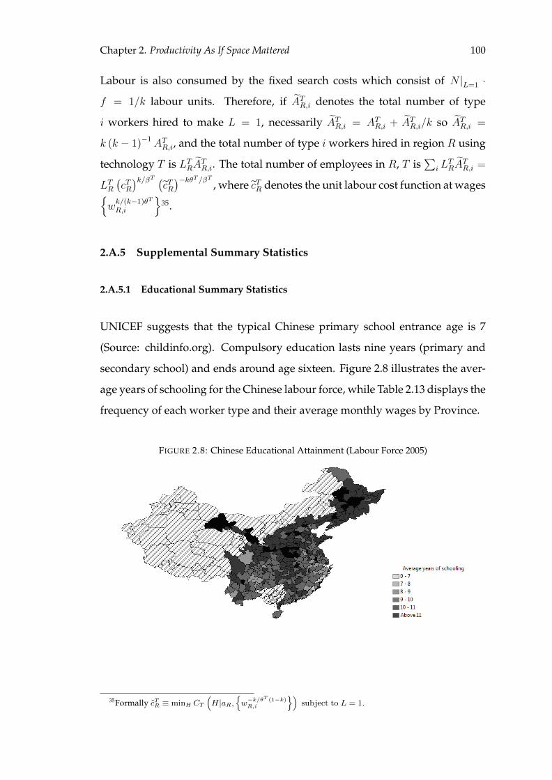
Chapter 2. Productivity As If Space Mattered 100
Labour is also consumed by the fixed search costs which consist of N |L=1 ·
f = 1/k labour units. Therefore, if ATR,i denotes the total number of type
i workers hired to make L = 1, necessarily ATR,i = ATR,i + ATR,i/k so ATR,i =
k (k − 1)−1ATR,i, and the total number of type i workers hired in region R using
technology T is LTRATR,i. The total number of employees in R, T is
∑i L
TRA
TR,i =
LTR(cTR)k/βT (
cTR)−kθT /βT , where cTR denotes the unit labour cost function at wages{
wk/(k−1)θTR,i
}35.
2.A.5 Supplemental Summary Statistics
2.A.5.1 Educational Summary Statistics
UNICEF suggests that the typical Chinese primary school entrance age is 7
(Source: childinfo.org). Compulsory education lasts nine years (primary and
secondary school) and ends around age sixteen. Figure 2.8 illustrates the aver-
age years of schooling for the Chinese labour force, while Table 2.13 displays the
frequency of each worker type and their average monthly wages by Province.
FIGURE 2.8: Chinese Educational Attainment (Labour Force 2005)
35Formally cTR ≡ minH CT(H|aR,
{w−k/θT (1−k)R,i
})subject to L = 1.
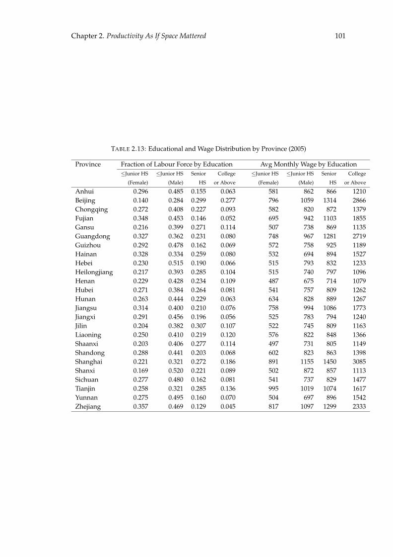
Chapter 2. Productivity As If Space Mattered 101
TABLE 2.13: Educational and Wage Distribution by Province (2005)
Province Fraction of Labour Force by Education Avg Monthly Wage by Education≤Junior HS ≤Junior HS Senior College ≤Junior HS ≤Junior HS Senior College
(Female) (Male) HS or Above (Female) (Male) HS or Above
Anhui 0.296 0.485 0.155 0.063 581 862 866 1210Beijing 0.140 0.284 0.299 0.277 796 1059 1314 2866Chongqing 0.272 0.408 0.227 0.093 582 820 872 1379Fujian 0.348 0.453 0.146 0.052 695 942 1103 1855Gansu 0.216 0.399 0.271 0.114 507 738 869 1135Guangdong 0.327 0.362 0.231 0.080 748 967 1281 2719Guizhou 0.292 0.478 0.162 0.069 572 758 925 1189Hainan 0.328 0.334 0.259 0.080 532 694 894 1527Hebei 0.230 0.515 0.190 0.066 515 793 832 1233Heilongjiang 0.217 0.393 0.285 0.104 515 740 797 1096Henan 0.229 0.428 0.234 0.109 487 675 714 1079Hubei 0.271 0.384 0.264 0.081 541 757 809 1262Hunan 0.263 0.444 0.229 0.063 634 828 889 1267Jiangsu 0.314 0.400 0.210 0.076 758 994 1086 1773Jiangxi 0.291 0.456 0.196 0.056 525 783 794 1240Jilin 0.204 0.382 0.307 0.107 522 745 809 1163Liaoning 0.250 0.410 0.219 0.120 576 822 848 1366Shaanxi 0.203 0.406 0.277 0.114 497 731 805 1149Shandong 0.288 0.441 0.203 0.068 602 823 863 1398Shanghai 0.221 0.321 0.272 0.186 891 1155 1450 3085Shanxi 0.169 0.520 0.221 0.089 502 872 857 1113Sichuan 0.277 0.480 0.162 0.081 541 737 829 1477Tianjin 0.258 0.321 0.285 0.136 995 1019 1074 1617Yunnan 0.275 0.495 0.160 0.070 504 697 896 1542Zhejiang 0.357 0.469 0.129 0.045 817 1097 1299 2333
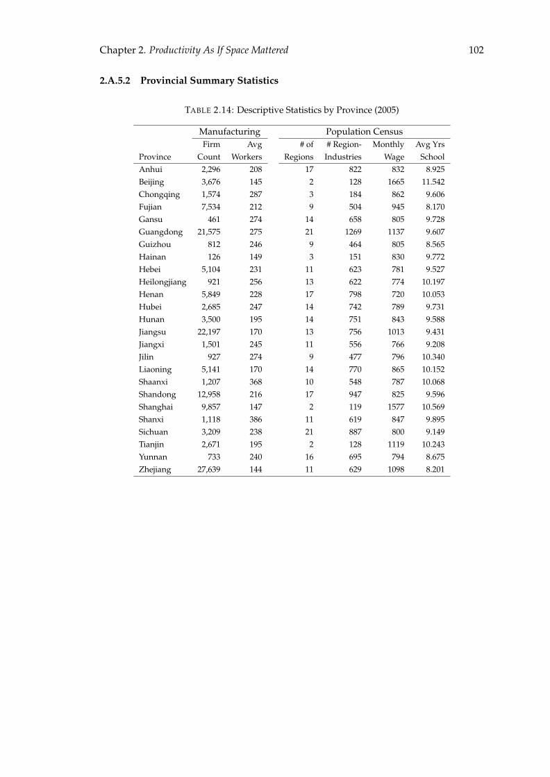
Chapter 2. Productivity As If Space Mattered 102
2.A.5.2 Provincial Summary Statistics
TABLE 2.14: Descriptive Statistics by Province (2005)
Manufacturing Population CensusFirm Avg # of # Region- Monthly Avg Yrs
Province Count Workers Regions Industries Wage SchoolAnhui 2,296 208 17 822 832 8.925Beijing 3,676 145 2 128 1665 11.542Chongqing 1,574 287 3 184 862 9.606Fujian 7,534 212 9 504 945 8.170Gansu 461 274 14 658 805 9.728Guangdong 21,575 275 21 1269 1137 9.607Guizhou 812 246 9 464 805 8.565Hainan 126 149 3 151 830 9.772Hebei 5,104 231 11 623 781 9.527Heilongjiang 921 256 13 622 774 10.197Henan 5,849 228 17 798 720 10.053Hubei 2,685 247 14 742 789 9.731Hunan 3,500 195 14 751 843 9.588Jiangsu 22,197 170 13 756 1013 9.431Jiangxi 1,501 245 11 556 766 9.208Jilin 927 274 9 477 796 10.340Liaoning 5,141 170 14 770 865 10.152Shaanxi 1,207 368 10 548 787 10.068Shandong 12,958 216 17 947 825 9.596Shanghai 9,857 147 2 119 1577 10.569Shanxi 1,118 386 11 619 847 9.895Sichuan 3,209 238 21 887 800 9.149Tianjin 2,671 195 2 128 1119 10.243Yunnan 733 240 16 695 794 8.675Zhejiang 27,639 144 11 629 1098 8.201
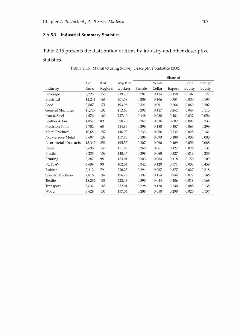
Chapter 2. Productivity As If Space Mattered 103
2.A.5.3 Industrial Summary Statistics
Table 2.15 presents the distribution of firms by industry and other descriptive
statistics.
TABLE 2.15: Manufacturing Survey Descriptive Statistics (2005)
Share of# of # of Avg # of White State Foreign
Industry firms Regions workers Female Collar Export Equity Equity
Beverage 2,225 155 219.20 0.281 0.114 0.150 0.107 0.121Electrical 12,241 166 201.58 0.289 0.106 0.351 0.030 0.195Food 3,807 171 193.98 0.321 0.091 0.266 0.060 0.202General Machines 15,727 195 152.68 0.205 0.117 0.262 0.047 0.115Iron & Steel 4,676 160 227.40 0.148 0.088 0.101 0.032 0.056Leather & Fur 4,852 89 320.70 0.362 0.036 0.682 0.005 0.335Precision Tools 2,702 68 214.89 0.296 0.180 0.457 0.063 0.299Metal Products 10,686 157 146.93 0.233 0.086 0.332 0.028 0.161Non-ferrous Metal 3,607 139 157.75 0.186 0.093 0.180 0.035 0.093Non-metal Products 15,347 259 195.57 0.207 0.090 0.169 0.059 0.088Paper 5,698 159 151.05 0.269 0.061 0.127 0.026 0.131Plastic 9,235 159 140.47 0.298 0.065 0.327 0.019 0.235Printing 3,382 98 133.01 0.303 0.084 0.118 0.150 0.109PC & AV 6,699 90 402.04 0.342 0.120 0.571 0.038 0.459Rubber 2,212 79 226.25 0.294 0.067 0.377 0.027 0.218Specific Machines 7,816 167 176.76 0.197 0.154 0.244 0.072 0.166Textile 18,292 186 222.43 0.390 0.044 0.406 0.018 0.168Transport 8,632 168 252.01 0.228 0.120 0.240 0.088 0.138Wood 3,629 133 137.04 0.288 0.050 0.290 0.025 0.137
Chapter 2. Productivity As If Space Mattered 104
2.A.6 Supplemental Empirical Results
2.A.6.1 Verisimilitude of Census and Firm Wages
One of the main concerns about combining census data with manufacturing
data is the representativeness of regional labour market conditions in determin-
ing actual wages within firms. It turns out they are remarkably good predictors
of a firm’s labour expenses. We construct a predictor of firm wages based on
Census data and test it as follows: First, compute the average wages per pre-
fecture. Second, make an estimate CensusWage by multiplying each firm’s dis-
tribution of workers by the average wages of each type from the population
census. Third, regress actual firm wages on CensusWage. The results are pre-
sented in Table 2.16 of Appendix 2.A.6.1. Not only is the R2 of this predictor
very high for each industry, but the coefficient on CensusWage is close to one
in all cases, showing that one-for-one the census based averages are excellent at
explaining the variation in the wage bill across firms.
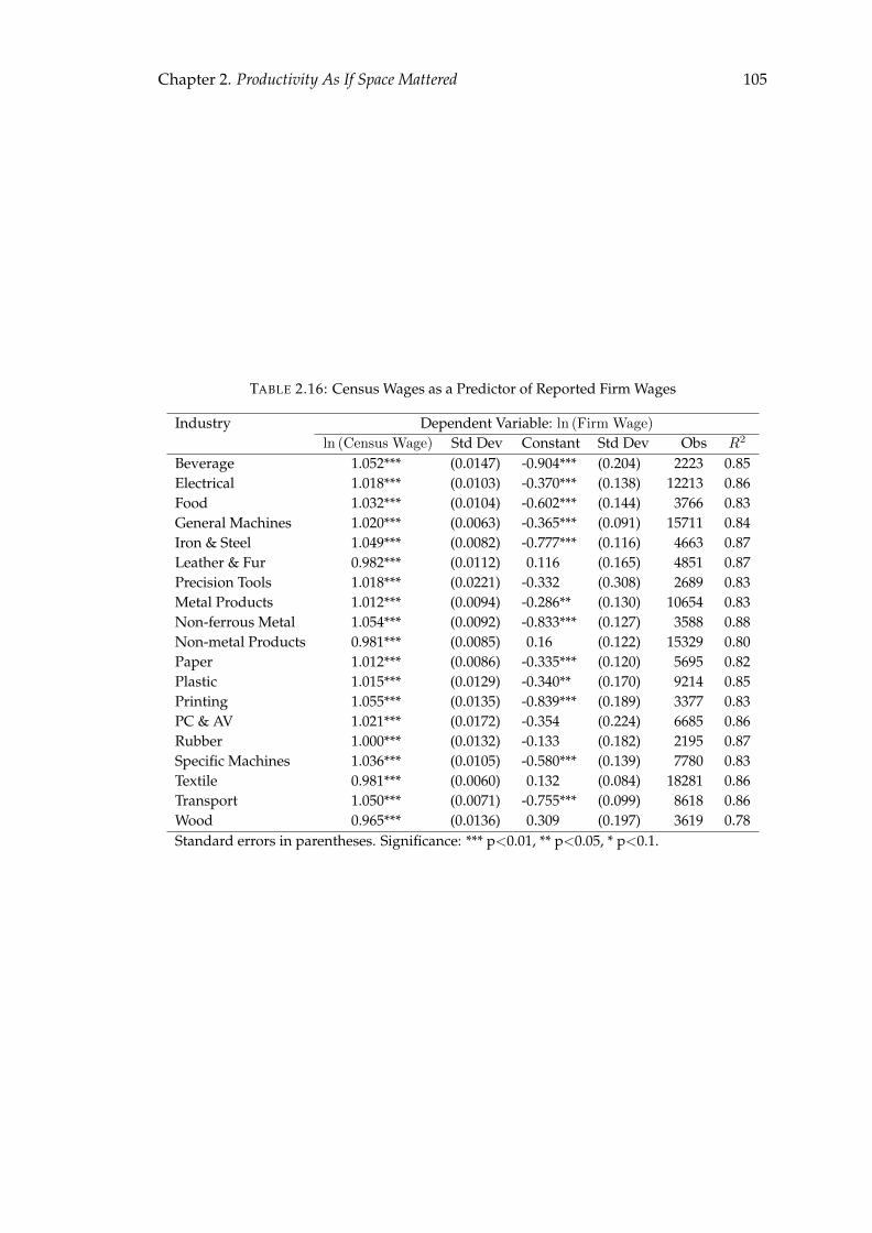
Chapter 2. Productivity As If Space Mattered 105
TABLE 2.16: Census Wages as a Predictor of Reported Firm Wages
Industry Dependent Variable: ln (Firm Wage)
ln (Census Wage) Std Dev Constant Std Dev Obs R2
Beverage 1.052*** (0.0147) -0.904*** (0.204) 2223 0.85Electrical 1.018*** (0.0103) -0.370*** (0.138) 12213 0.86Food 1.032*** (0.0104) -0.602*** (0.144) 3766 0.83General Machines 1.020*** (0.0063) -0.365*** (0.091) 15711 0.84Iron & Steel 1.049*** (0.0082) -0.777*** (0.116) 4663 0.87Leather & Fur 0.982*** (0.0112) 0.116 (0.165) 4851 0.87Precision Tools 1.018*** (0.0221) -0.332 (0.308) 2689 0.83Metal Products 1.012*** (0.0094) -0.286** (0.130) 10654 0.83Non-ferrous Metal 1.054*** (0.0092) -0.833*** (0.127) 3588 0.88Non-metal Products 0.981*** (0.0085) 0.16 (0.122) 15329 0.80Paper 1.012*** (0.0086) -0.335*** (0.120) 5695 0.82Plastic 1.015*** (0.0129) -0.340** (0.170) 9214 0.85Printing 1.055*** (0.0135) -0.839*** (0.189) 3377 0.83PC & AV 1.021*** (0.0172) -0.354 (0.224) 6685 0.86Rubber 1.000*** (0.0132) -0.133 (0.182) 2195 0.87Specific Machines 1.036*** (0.0105) -0.580*** (0.139) 7780 0.83Textile 0.981*** (0.0060) 0.132 (0.084) 18281 0.86Transport 1.050*** (0.0071) -0.755*** (0.099) 8618 0.86Wood 0.965*** (0.0136) 0.309 (0.197) 3619 0.78Standard errors in parentheses. Significance: *** p<0.01, ** p<0.05, * p<0.1.
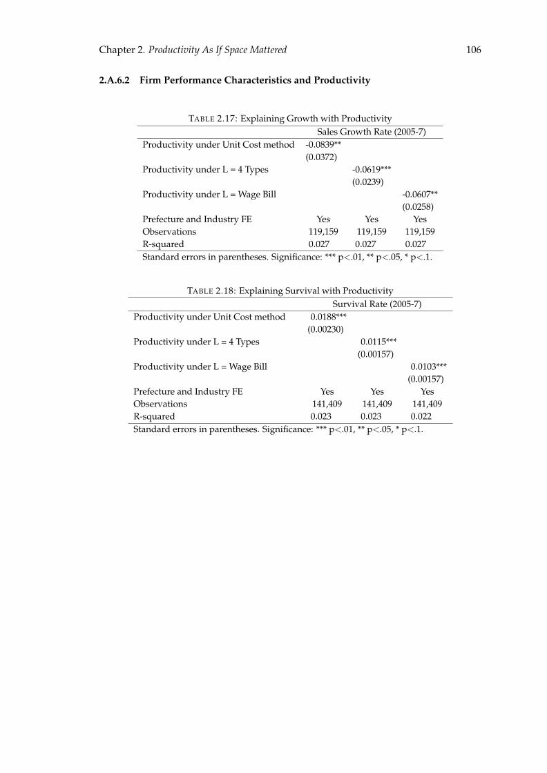
Chapter 2. Productivity As If Space Mattered 106
2.A.6.2 Firm Performance Characteristics and Productivity
TABLE 2.17: Explaining Growth with ProductivitySales Growth Rate (2005-7)
Productivity under Unit Cost method -0.0839**(0.0372)
Productivity under L = 4 Types -0.0619***(0.0239)
Productivity under L = Wage Bill -0.0607**(0.0258)
Prefecture and Industry FE Yes Yes YesObservations 119,159 119,159 119,159R-squared 0.027 0.027 0.027Standard errors in parentheses. Significance: *** p<.01, ** p<.05, * p<.1.
TABLE 2.18: Explaining Survival with ProductivitySurvival Rate (2005-7)
Productivity under Unit Cost method 0.0188***(0.00230)
Productivity under L = 4 Types 0.0115***(0.00157)
Productivity under L = Wage Bill 0.0103***(0.00157)
Prefecture and Industry FE Yes Yes YesObservations 141,409 141,409 141,409R-squared 0.023 0.023 0.022Standard errors in parentheses. Significance: *** p<.01, ** p<.05, * p<.1.
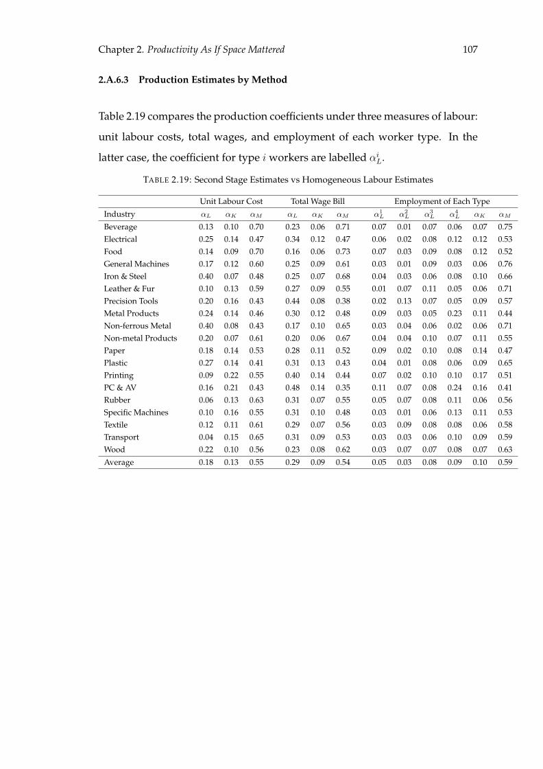
Chapter 2. Productivity As If Space Mattered 107
2.A.6.3 Production Estimates by Method
Table 2.19 compares the production coefficients under three measures of labour:
unit labour costs, total wages, and employment of each worker type. In the
latter case, the coefficient for type i workers are labelled αiL.
TABLE 2.19: Second Stage Estimates vs Homogeneous Labour Estimates
Unit Labour Cost Total Wage Bill Employment of Each Type
Industry αL αK αM αL αK αM α1L α2
L α3L α4
L αK αM
Beverage 0.13 0.10 0.70 0.23 0.06 0.71 0.07 0.01 0.07 0.06 0.07 0.75Electrical 0.25 0.14 0.47 0.34 0.12 0.47 0.06 0.02 0.08 0.12 0.12 0.53Food 0.14 0.09 0.70 0.16 0.06 0.73 0.07 0.03 0.09 0.08 0.12 0.52General Machines 0.17 0.12 0.60 0.25 0.09 0.61 0.03 0.01 0.09 0.03 0.06 0.76Iron & Steel 0.40 0.07 0.48 0.25 0.07 0.68 0.04 0.03 0.06 0.08 0.10 0.66Leather & Fur 0.10 0.13 0.59 0.27 0.09 0.55 0.01 0.07 0.11 0.05 0.06 0.71Precision Tools 0.20 0.16 0.43 0.44 0.08 0.38 0.02 0.13 0.07 0.05 0.09 0.57Metal Products 0.24 0.14 0.46 0.30 0.12 0.48 0.09 0.03 0.05 0.23 0.11 0.44Non-ferrous Metal 0.40 0.08 0.43 0.17 0.10 0.65 0.03 0.04 0.06 0.02 0.06 0.71Non-metal Products 0.20 0.07 0.61 0.20 0.06 0.67 0.04 0.04 0.10 0.07 0.11 0.55Paper 0.18 0.14 0.53 0.28 0.11 0.52 0.09 0.02 0.10 0.08 0.14 0.47Plastic 0.27 0.14 0.41 0.31 0.13 0.43 0.04 0.01 0.08 0.06 0.09 0.65Printing 0.09 0.22 0.55 0.40 0.14 0.44 0.07 0.02 0.10 0.10 0.17 0.51PC & AV 0.16 0.21 0.43 0.48 0.14 0.35 0.11 0.07 0.08 0.24 0.16 0.41Rubber 0.06 0.13 0.63 0.31 0.07 0.55 0.05 0.07 0.08 0.11 0.06 0.56Specific Machines 0.10 0.16 0.55 0.31 0.10 0.48 0.03 0.01 0.06 0.13 0.11 0.53Textile 0.12 0.11 0.61 0.29 0.07 0.56 0.03 0.09 0.08 0.08 0.06 0.58Transport 0.04 0.15 0.65 0.31 0.09 0.53 0.03 0.03 0.06 0.10 0.09 0.59Wood 0.22 0.10 0.56 0.23 0.08 0.62 0.03 0.07 0.07 0.08 0.07 0.63
Average 0.18 0.13 0.55 0.29 0.09 0.54 0.05 0.03 0.08 0.09 0.10 0.59

Chapter 3
Education, Occupation and
Children’s Outcomes: The Impact of
the Chinese Cultural Revolution
3.1 Introduction
Previous studies find that an increase in the availability of schooling raises ed-
ucational attainment, which in turn reduces poverty and improves social mo-
bility.1 Higher educational attainment leads to better labour market outcomes,
such as higher income and occupational status, and may have positive long-
run effects on children’s school performance. Therefore, many countries have
carried out various reforms to improve the access to education.2 In developing
countries where early school drop-out rates are high, more emphasis is given1See Birdsall (1985); Lavy (1996); Duflo (2001) for examples of the impact of education policy on school-
ing. Studies on the link between education reform and intergenerational mobility include Black et al.(2005); Pekkarinen et al. (2006); Holmlund (2008) and Maurin and McNally (2008).
2Examples of large-scale education reform in developing countries include the massive school con-struction in Indonesia in the 1970s and in India in the 1990s; the implementation of a compulsory schoolinglaw in China in 1986; and the provision of free primary education in Kenya in 2003.
108

Chapter 3. Education, Occupation and Children’s Outcomes 109
to the expansion of basic education as it benefits a larger social group and im-
proves social mobility at the bottom of the income distribution.3
By exploiting the drastic education reform during the Chinese Cultural Rev-
olution, this paper examines how changes in access to basic education affect
schooling and their subsequent impact on occupational choice and children’s
educational attainment. In 1968-1976, a revolutionary education agenda was
implemented in China to remove class differences and social inequality. In ur-
ban schools, ability tracks were abolished, schooling was restructured and the
curriculum was simplified to increase the grade progression rate among prole-
tarian families. New primary schools were built in rural areas to universalise
education among the agricultural population. Although the quality of educa-
tion suffered throughout the period, the new policies led to a significant rise in
school enrolment and graduation rates. Between 1962 and 1975, primary and
junior high school enrolment rates increased from 56.1% and 45.3% to 96.8%
and 90% respectively (Ministry of Education).
The education reform in 1968-76 resulted in an exogenous change in the ed-
ucational distribution among the school-aged cohorts, and the reform intensity
was uneven across regions as different policies were adopted by the local gov-
ernments. Using trend deviations of graduation rate as a proxy of education
shock, I find that cohorts born in 1950-65 were most affected by the educa-
tion reform and the impact was largest at primary and junior high school lev-
els.4 Moreover, the deviations from education trend varied significantly across3Investment in higher education favours those with larger family endowment, and therefore has little
redistributional effects. In fact, a number of studies suggest that reforms that promote equity in educationimprove intergenerational mobility (e.g. Holmlund (2008) and Pekkarinen et al. (2006)). Policies such asextension of compulsory years of schooling, abolishment of ability tracking system and introduction ofstandardised academic curriculum reduce intergenerational correlations in education and income.
4I do not consider the impact of university closure on educational attainment as less than 1% of theschool-aged children entered university before the Cultural Revolution and most of them were from theelite class; therefore, the effect was confined to a very small group of people.

Chapter 3. Education, Occupation and Children’s Outcomes 110
provinces and hukou type.5 I use this variation in trend deviations as an in-
strument for individual’s schooling to estimate the impact of education on oc-
cupational status and children’s schooling outcomes. The key assumption of
this identification strategy is the estimated education shock is uncorrelated with
other regional characteristics that affect the individual’s educational decision.
The results suggest that schooling has positive and significant impact on the
status of first occupation and children’s educational attainment. Each addi-
tional year of schooling increases the probability of obtaining an off-farm job
by 3.11%, and increases the likelihood of acquiring a white collar job by 2.87%.
Moreover, increasing parent’s education by one year increases children’s prob-
ability of completing junior high school and senior high school by 3.94% and
4.76% respectively.
This study is closely related to an existing literature which uses changes
in education policy to identify the causal relationship between schooling and
labour market outcomes. For example, Duflo (2001) finds that individual’s ed-
ucation increases by 0.12-0.19 years for each new school built per 1000 chil-
dren in Indonesia and generates returns to education of 6.8-10.6%. Maurin
and McNally (2008) show that the temporary relaxation of French university
entrance exam in 1968 led to an increase in years of higher education, which
consequently increased wages and occupational status. Some studies also use
changes in education system to examine the relationship between parents’ and
children’s education. Maurin and McNally (2008) find that higher parental ed-
ucation reduces children’s years of grade repetition in France. Oreopoulos et al.
(2006) use changes in compulsory schooling law in the US as an instrument
for parental education and find positive and significant effects of parental ed-
ucation on children’s school performance. Black et al. (2005) adopt a similar
approach and finds little causal relationship between parent’s and children’s
education in Norway.5A person’s hukou type defines his region of permanent residence (urban or rural) and family’s occu-
pation (agricultural or non-agricultural). However, the link between one’s hukou type and occupation israther weak after the mid-1990s.
Chapter 3. Education, Occupation and Children’s Outcomes 111
Finally, this paper is also related to a recent literature which uses the Cul-
tural Revolution as a natural experiment to estimate the returns to education
in China. Meng and Gregory (2007) use year of birth as an instrument for ed-
ucation disruption to estimate the education cost of the Cultural Revolution.
They find that the impact of missed years of schooling or lack of normal cur-
riculum on earnings is very small. The major disadvantage of their approach
is they assume that the treatment intensity is the same within the cohorts, and
therefore fail to exploit the regional variation in the education shock. In order
to capture this variation, Giles et al. (2008) estimate the returns to education in
urban China using city-wide birth-cohort average disruption to education as an
instrument for schooling. They find that the IV estimate of returns to education
was about 13%, much higher than the OLS estimate of 8%, which suggests that
there was an under-investment in education in China.
The rest of the paper is organised as follows. Section 2 explains the back-
ground of the Cultural Revolution; Section 3 discusses the conceptual frame-
work; and Section 4 describes the empirical strategy. Section 5 presents the
empirical results and Section 6 concludes.
3.2 Background
3.2.1 Education System and Cultural Revolution
Before the Cultural Revolution, China’s education system was characterised by
a combination of academic and vocational schools to produce trained experts
and educated labourers (Tsang, 2000). Rapid expansion of education among
peasants and proletariat families was observed earlier in 1958-61; however, the
government reverted to a more practical education policy after the failure of
the Great Leap Forward in 1961. To make efficient use of the limited resources,
urban schools were given priority over their rural counterparts to train special-
ists for the country’s development goals. In urban ’key-point’ schools, expertise

Chapter 3. Education, Occupation and Children’s Outcomes 112
was emphasized and competition for progression was tight. In contrast, the aim
of rural education was to eradicate adult illiteracy and produce educated work-
ers for agricultural production. Grade durations were shorter and educational
quality was lower. Such regional disparities in education were reinforced by the
hukou system which imposed huge institutional and monetary costs on migra-
tion, and therefore deprived rural households from higher quality education in
urban areas.
The earlier education system was abruptly abolished after the outbreak of
the Cultural Revolution. In 1966-68, urban schools were closed and normal
teaching was suspended so that students could dedicate themselves to politi-
cal activities. As one of the aims of the Cultural Revolution was to promote
egalitarianism, a new education agenda was adopted in 1968 to provide peas-
ants and proletarians with better educational opportunities. In primary and
secondary schools, the education structure was unified and school curriculum
was simplified to reduce the gaps between students from different social back-
grounds. Normal school lessons were replaced by political and ideological ed-
ucation and manual farm work. To increase school progression rates, exams
were abolished and students were given diplomas even though they missed
schooling due to the initial school closure.6 In rural areas, villages were pushed
to build new schools and expand schooling to junior high school level (Tsang,
2000). Although teaching quality and school conditions were poor, the reform
was quite successful in promoting mass education in rural areas. Between 1965
and 1976, rural enrolments in primary and junior high school increased from
80.9% to 88.5% and 30.2% to 72% respectively (Ministry of Education). It was
not until 1977 that all schools returned to normal operations.6The loss in university education was also tremendous during the Cultural Revolution. Many uni-
versity professors were sent to the country-side for re-education and no formal teaching was undertakenthroughout the period. Only a small number of students were recruited after 1972 on the basis of politicalattitude and social background. As only a very small fraction of population enters university before theoutbreak of Cultural Revolution; therefore my analysis focuses on the initial interruption and subsequentexpansion of primary and secondary education.

Chapter 3. Education, Occupation and Children’s Outcomes 113
3.2.2 Impact on Schooling
This section discusses the factors that affect schooling decisions and how they
are related to the education reform during the Cultural Revolution. The classi-
cal human capital theory suggests that investment in education is affected by
four main factors: ability, returns to education, cost of schooling, and household
liquidity constraint if there is imperfect capital market.7 Either an increase in
ability, parental income and returns to education, or decrease in cost of school-
ing would increase investment in schooling, holding other things constant.
The initial school closure in 1966-68 was a negative education shock to school-
aged children, especially among those who lived in the urban areas or had
an non-agricultural hukou. Although most schools were reopened in 1968, all
’key-point’ schools and vocational schools remained closed throughout the pe-
riod. Students might drop out of school permanently if they find it not worth-
while to re-enter schools after 1968, and these students tend to have higher cost
of schooling or lower returns to education than their peers.
The subsequent education reform in 1968-76 can affect an individual’s edu-
cation decision in three ways. First, the abolition of exams and the change in
school curriculum reduce the cost of effort for grade progression, which there-
fore increases the education level of students. Second, construction of new pri-
mary schools in rural areas reduces the cost of education and consequently in-
creases the investment in education among the liquidity constrained families.
Third, the poor teaching quality and removal of link between education and
future earnings reduces the returns to education. Education no longer serves
as a signalling device in the labour market and urban high school graduates
were assigned to jobs directly by the government. Many of them were sent to7See Becker (1962) and Becker and Tomes (1986) for a detailed discussion of the human capital model.

Chapter 3. Education, Occupation and Children’s Outcomes 114
the countryside to work as peasants as there were insufficient jobs in the urban
areas. This reduces the incentive to invest in education.8
The relative magnitude of the three effects depends on an individual’s re-
gion of residence and family background. Under an exam-based system, stu-
dents with a lower cost of exam preparation are more likely to progress to a
higher grade. As children of intellectuals and government officials are best-
equipped for the exams, they tend to have higher education levels than their
peers. The removal of ability tracks reduces the importance of academic ability
in determining schooling outcomes, which favours children from proletarian
families. Next, primary school construction explicitly targeted areas where il-
literacy rate was high and educational opportunities were limited. This would
increase the educational level of the poor and narrow the education gap across
regions. The impact of decline in returns to education is ambiguous. If labour
market outcomes are independent of a student’s academic performance during
the Cultural Revolution, then the fall in returns to education is larger at higher
education levels and education inequality would decrease.9
3.2.3 Variation in Treatment Intensity
There are two sources of variation in treatment intensity. The first one is year
of birth. Cohorts affected by the reform ranged from students who attended
senior high school in 1968 to children who were about to complete primary
education in 1976. In China, children started primary schools at the age of 7 and
completed senior high school at 18. Therefore, the treatment groups include 16
birth cohorts born between 1950 and 1965. The 1950-54 cohorts attended junior
and/or senior high school during the Cultural Revolution; the 1955-59 cohorts8Another factor that affects schooling decision but not related to the education reform is the struggle
against intellectuals. During the Cultural Revolution, many intellectuals faced a negative income shockas their property was confiscated and their families were sent to rural areas for re-education. This reducestheir demand for children’s education if education is a normal good.
9Another policy that contributes to the reduction in education disparities is the disruption in univer-sity education which hinders children of intellectuals from obtaining higher education. When universitiesstarted recruiting a small number of new students in 1972, only those from peasants and proletarian fam-ilies or closely related to government officials were recruited.
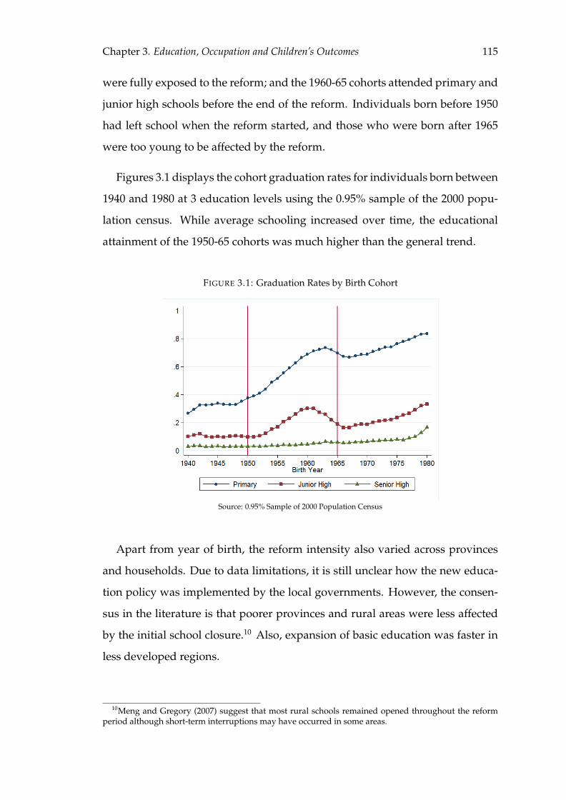
Chapter 3. Education, Occupation and Children’s Outcomes 115
were fully exposed to the reform; and the 1960-65 cohorts attended primary and
junior high schools before the end of the reform. Individuals born before 1950
had left school when the reform started, and those who were born after 1965
were too young to be affected by the reform.
Figures 3.1 displays the cohort graduation rates for individuals born between
1940 and 1980 at 3 education levels using the 0.95% sample of the 2000 popu-
lation census. While average schooling increased over time, the educational
attainment of the 1950-65 cohorts was much higher than the general trend.
FIGURE 3.1: Graduation Rates by Birth Cohort
Source: 0.95% Sample of 2000 Population Census
Apart from year of birth, the reform intensity also varied across provinces
and households. Due to data limitations, it is still unclear how the new educa-
tion policy was implemented by the local governments. However, the consen-
sus in the literature is that poorer provinces and rural areas were less affected
by the initial school closure.10 Also, expansion of basic education was faster in
less developed regions.
10Meng and Gregory (2007) suggest that most rural schools remained opened throughout the reformperiod although short-term interruptions may have occurred in some areas.
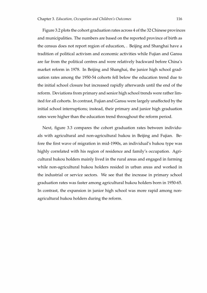
Chapter 3. Education, Occupation and Children’s Outcomes 116
Figure 3.2 plots the cohort graduation rates across 4 of the 32 Chinese provinces
and municipalities. The numbers are based on the reported province of birth as
the census does not report region of education, . Beijing and Shanghai have a
tradition of political activism and economic activities while Fujian and Gansu
are far from the political centres and were relatively backward before China’s
market reform in 1978. In Beijing and Shanghai, the junior high school grad-
uation rates among the 1950-54 cohorts fell below the education trend due to
the initial school closure but increased rapidly afterwards until the end of the
reform. Deviations from primary and senior high school trends were rather lim-
ited for all cohorts. In contrast, Fujian and Gansu were largely unaffected by the
initial school interruptions; instead, their primary and junior high graduation
rates were higher than the education trend throughout the reform period.
Next, figure 3.3 compares the cohort graduation rates between individu-
als with agricultural and non-agricultural hukou in Beijing and Fujian. Be-
fore the first wave of migration in mid-1990s, an individual’s hukou type was
highly correlated with his region of residence and family’s occupation. Agri-
cultural hukou holders mainly lived in the rural areas and engaged in farming
while non-agricultural hukou holders resided in urban areas and worked in
the industrial or service sectors. We see that the increase in primary school
graduation rates was faster among agricultural hukou holders born in 1950-65.
In contrast, the expansion in junior high school was more rapid among non-
agricultural hukou holders during the reform.
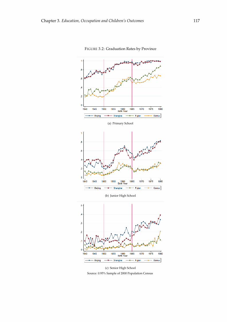
Chapter 3. Education, Occupation and Children’s Outcomes 117
FIGURE 3.2: Graduation Rates by Province
(a) Primary School
(b) Junior High School
(c) Senior High School
Source: 0.95% Sample of 2000 Population Census
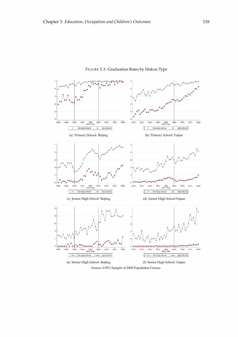
Chapter 3. Education, Occupation and Children’s Outcomes 118
FIGURE 3.3: Graduation Rates by Hukou Type
(a) Primary School: Beijing (b) Primary School: Fujian
(c) Junior High School: Beijing (d) Junior High School Fujian
(e) Senior High School: Beijing (f) Senior High School: Fujian
Source: 0.95% Sample of 2000 Population Census
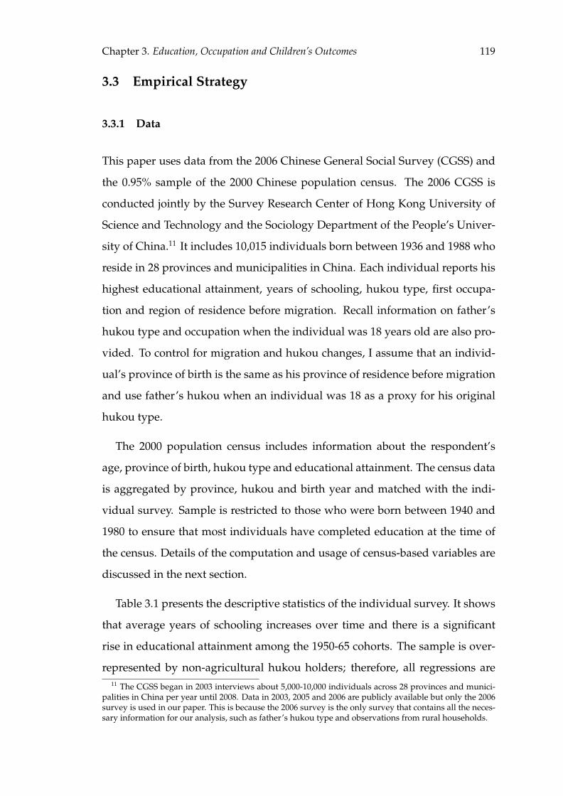
Chapter 3. Education, Occupation and Children’s Outcomes 119
3.3 Empirical Strategy
3.3.1 Data
This paper uses data from the 2006 Chinese General Social Survey (CGSS) and
the 0.95% sample of the 2000 Chinese population census. The 2006 CGSS is
conducted jointly by the Survey Research Center of Hong Kong University of
Science and Technology and the Sociology Department of the People’s Univer-
sity of China.11 It includes 10,015 individuals born between 1936 and 1988 who
reside in 28 provinces and municipalities in China. Each individual reports his
highest educational attainment, years of schooling, hukou type, first occupa-
tion and region of residence before migration. Recall information on father’s
hukou type and occupation when the individual was 18 years old are also pro-
vided. To control for migration and hukou changes, I assume that an individ-
ual’s province of birth is the same as his province of residence before migration
and use father’s hukou when an individual was 18 as a proxy for his original
hukou type.
The 2000 population census includes information about the respondent’s
age, province of birth, hukou type and educational attainment. The census data
is aggregated by province, hukou and birth year and matched with the indi-
vidual survey. Sample is restricted to those who were born between 1940 and
1980 to ensure that most individuals have completed education at the time of
the census. Details of the computation and usage of census-based variables are
discussed in the next section.
Table 3.1 presents the descriptive statistics of the individual survey. It shows
that average years of schooling increases over time and there is a significant
rise in educational attainment among the 1950-65 cohorts. The sample is over-
represented by non-agricultural hukou holders; therefore, all regressions are11 The CGSS began in 2003 interviews about 5,000-10,000 individuals across 28 provinces and munici-
palities in China per year until 2008. Data in 2003, 2005 and 2006 are publicly available but only the 2006survey is used in our paper. This is because the 2006 survey is the only survey that contains all the neces-sary information for our analysis, such as father’s hukou type and observations from rural households.
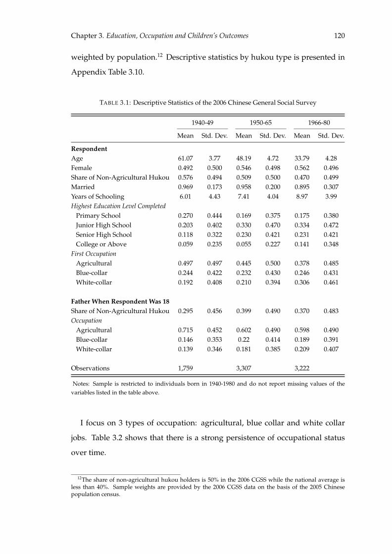
Chapter 3. Education, Occupation and Children’s Outcomes 120
weighted by population.12 Descriptive statistics by hukou type is presented in
Appendix Table 3.10.
TABLE 3.1: Descriptive Statistics of the 2006 Chinese General Social Survey
1940-49 1950-65 1966-80
Mean Std. Dev. Mean Std. Dev. Mean Std. Dev.
RespondentAge 61.07 3.77 48.19 4.72 33.79 4.28Female 0.492 0.500 0.546 0.498 0.562 0.496Share of Non-Agricultural Hukou 0.576 0.494 0.509 0.500 0.470 0.499Married 0.969 0.173 0.958 0.200 0.895 0.307Years of Schooling 6.01 4.43 7.41 4.04 8.97 3.99Highest Education Level Completed
Primary School 0.270 0.444 0.169 0.375 0.175 0.380Junior High School 0.203 0.402 0.330 0.470 0.334 0.472Senior High School 0.118 0.322 0.230 0.421 0.231 0.421College or Above 0.059 0.235 0.055 0.227 0.141 0.348
First OccupationAgricultural 0.497 0.497 0.445 0.500 0.378 0.485Blue-collar 0.244 0.422 0.232 0.430 0.246 0.431White-collar 0.192 0.408 0.210 0.394 0.306 0.461
Father When Respondent Was 18Share of Non-Agricultural Hukou 0.295 0.456 0.399 0.490 0.370 0.483Occupation
Agricultural 0.715 0.452 0.602 0.490 0.598 0.490Blue-collar 0.146 0.353 0.22 0.414 0.189 0.391White-collar 0.139 0.346 0.181 0.385 0.209 0.407
Observations 1,759 3,307 3,222
Notes: Sample is restricted to individuals born in 1940-1980 and do not report missing values of thevariables listed in the table above.
I focus on 3 types of occupation: agricultural, blue collar and white collar
jobs. Table 3.2 shows that there is a strong persistence of occupational status
over time.
12The share of non-agricultural hukou holders is 50% in the 2006 CGSS while the national average isless than 40%. Sample weights are provided by the 2006 CGSS data on the basis of the 2005 Chinesepopulation census.
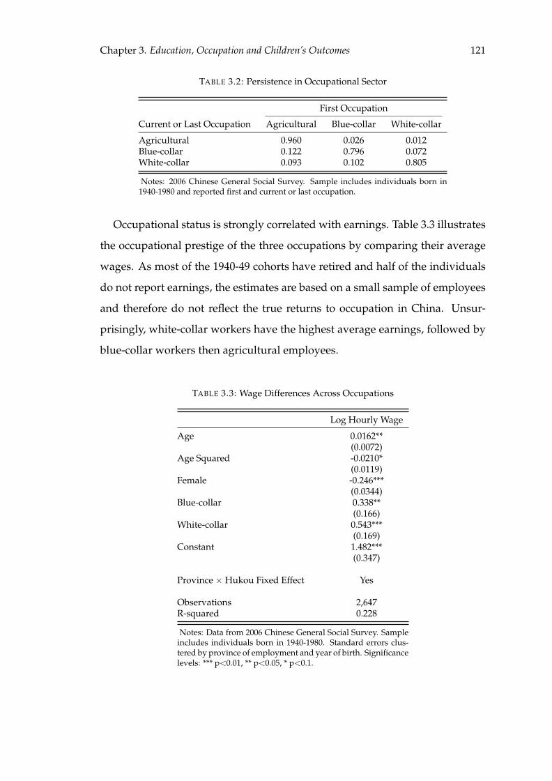
Chapter 3. Education, Occupation and Children’s Outcomes 121
TABLE 3.2: Persistence in Occupational Sector
First Occupation
Current or Last Occupation Agricultural Blue-collar White-collar
Agricultural 0.960 0.026 0.012Blue-collar 0.122 0.796 0.072White-collar 0.093 0.102 0.805
Notes: 2006 Chinese General Social Survey. Sample includes individuals born in1940-1980 and reported first and current or last occupation.
Occupational status is strongly correlated with earnings. Table 3.3 illustrates
the occupational prestige of the three occupations by comparing their average
wages. As most of the 1940-49 cohorts have retired and half of the individuals
do not report earnings, the estimates are based on a small sample of employees
and therefore do not reflect the true returns to occupation in China. Unsur-
prisingly, white-collar workers have the highest average earnings, followed by
blue-collar workers then agricultural employees.
TABLE 3.3: Wage Differences Across Occupations
Log Hourly Wage
Age 0.0162**(0.0072)
Age Squared -0.0210*(0.0119)
Female -0.246***(0.0344)
Blue-collar 0.338**(0.166)
White-collar 0.543***(0.169)
Constant 1.482***(0.347)
Province × Hukou Fixed Effect Yes
Observations 2,647R-squared 0.228
Notes: Data from 2006 Chinese General Social Survey. Sampleincludes individuals born in 1940-1980. Standard errors clus-tered by province of employment and year of birth. Significancelevels: *** p<0.01, ** p<0.05, * p<0.1.
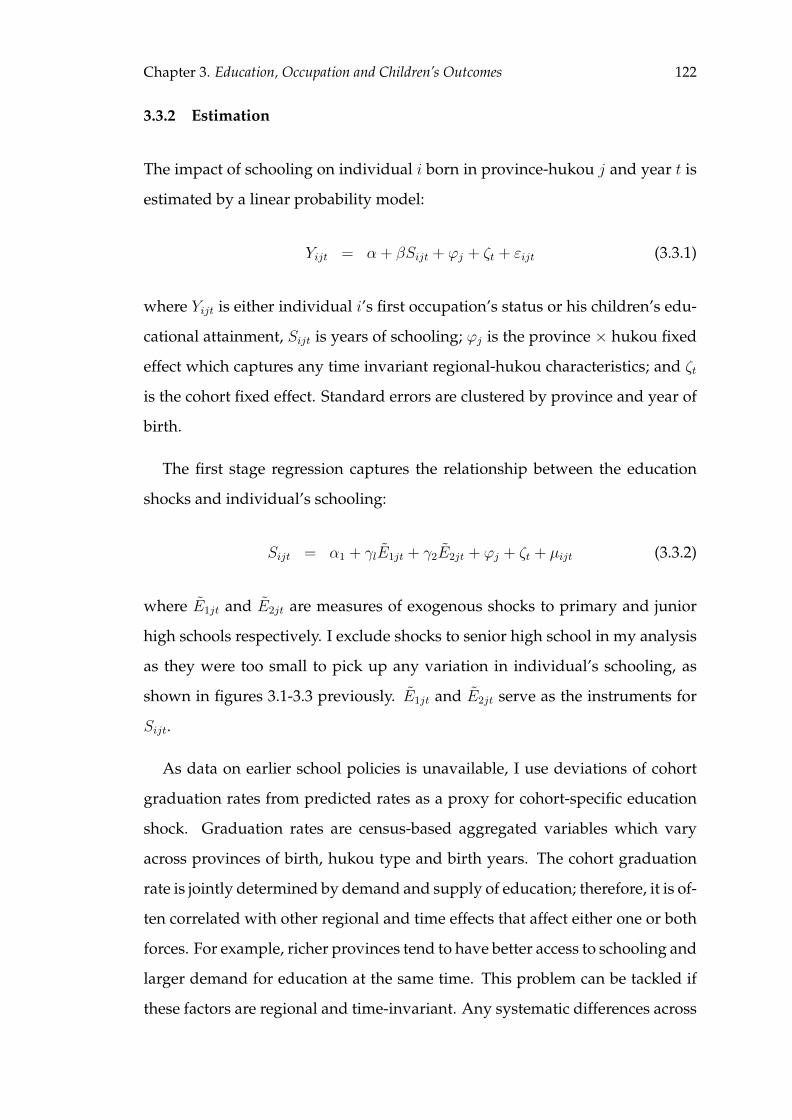
Chapter 3. Education, Occupation and Children’s Outcomes 122
3.3.2 Estimation
The impact of schooling on individual i born in province-hukou j and year t is
estimated by a linear probability model:
Yijt = α + βSijt + ϕj + ζt + εijt (3.3.1)
where Yijt is either individual i’s first occupation’s status or his children’s edu-
cational attainment, Sijt is years of schooling; ϕj is the province × hukou fixed
effect which captures any time invariant regional-hukou characteristics; and ζt
is the cohort fixed effect. Standard errors are clustered by province and year of
birth.
The first stage regression captures the relationship between the education
shocks and individual’s schooling:
Sijt = α1 + γlE1jt + γ2E2jt + ϕj + ζt + µijt (3.3.2)
where E1jt and E2jt are measures of exogenous shocks to primary and junior
high schools respectively. I exclude shocks to senior high school in my analysis
as they were too small to pick up any variation in individual’s schooling, as
shown in figures 3.1-3.3 previously. E1jt and E2jt serve as the instruments for
Sijt.
As data on earlier school policies is unavailable, I use deviations of cohort
graduation rates from predicted rates as a proxy for cohort-specific education
shock. Graduation rates are census-based aggregated variables which vary
across provinces of birth, hukou type and birth years. The cohort graduation
rate is jointly determined by demand and supply of education; therefore, it is of-
ten correlated with other regional and time effects that affect either one or both
forces. For example, richer provinces tend to have better access to schooling and
larger demand for education at the same time. This problem can be tackled if
these factors are regional and time-invariant. Any systematic differences across
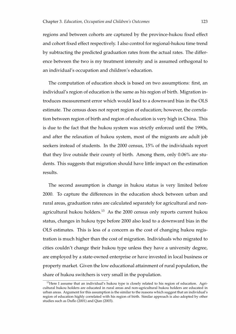
Chapter 3. Education, Occupation and Children’s Outcomes 123
regions and between cohorts are captured by the province-hukou fixed effect
and cohort fixed effect respectively. I also control for regional-hukou time trend
by subtracting the predicted graduation rates from the actual rates. The differ-
ence between the two is my treatment intensity and is assumed orthogonal to
an individual’s occupation and children’s education.
The computation of education shock is based on two assumptions: first, an
individual’s region of education is the same as his region of birth. Migration in-
troduces measurement error which would lead to a downward bias in the OLS
estimate. The census does not report region of education; however, the correla-
tion between region of birth and region of education is very high in China. This
is due to the fact that the hukou system was strictly enforced until the 1990s,
and after the relaxation of hukou system, most of the migrants are adult job
seekers instead of students. In the 2000 census, 15% of the individuals report
that they live outside their county of birth. Among them, only 0.06% are stu-
dents. This suggests that migration should have little impact on the estimation
results.
The second assumption is change in hukou status is very limited before
2000. To capture the differences in the education shock between urban and
rural areas, graduation rates are calculated separately for agricultural and non-
agricultural hukou holders.13 As the 2000 census only reports current hukou
status, changes in hukou type before 2000 also lead to a downward bias in the
OLS estimates. This is less of a concern as the cost of changing hukou regis-
tration is much higher than the cost of migration. Individuals who migrated to
cities couldn’t change their hukou type unless they have a university degree,
are employed by a state-owned enterprise or have invested in local business or
property market. Given the low educational attainment of rural population, the
share of hukou switchers is very small in the population.13Here I assume that an individual’s hukou type is closely related to his region of education. Agri-
cultural hukou holders are educated in rural areas and non-agricultural hukou holders are educated inurban areas. Argument for this assumption is the similar to the reasons which suggest that an individual’sregion of education highly correlated with his region of birth. Similar approach is also adopted by otherstudies such as Duflo (2001) and Qian (2003).

Chapter 3. Education, Occupation and Children’s Outcomes 124
The education trend of each cohort group is estimated by the following equa-
tion:
Eljt = αlj + θ1ljElj1940 × [t− 1940] + θ2ljElj1940 × [t− 1940]2 + νjt (3.3.3)
where Eljt is the actual graduation rate of education level l for each province,
hukou and birth cohort, and Ejk1940 is the graduation rate of the 1940 cohort.
θ2lj captures the non-linear trends in educational attainment across cohorts.
The instrumental variable Eljt is defined as the difference between the actual
and predicted graduation rates. In order to isolate the education shocks dur-
ing the Cultural Revolution, equation (3.3.3) is estimated for the control group
only i.e. the 1940-49 and 1966-80 cohorts. Figure 3.4 presents the histograms
of estimated trend deviations for three education levels. Each observation is a
province, hukou and birth year cell. It suggests that education shock is larger
for the 1950-65 birth cohorts and for primary schools and junior high schools. A
breakdown of Figure 3.4 by hukou type is also shown in Appendix Figure 3.5.
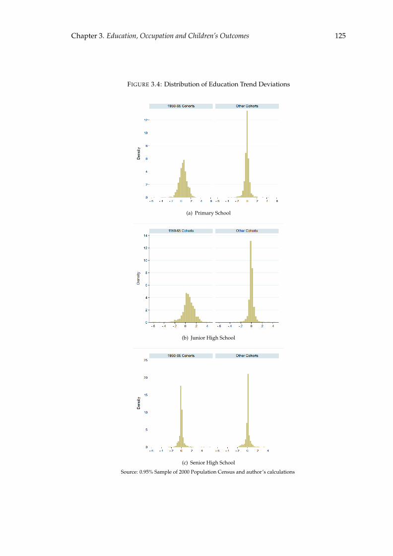
Chapter 3. Education, Occupation and Children’s Outcomes 125
FIGURE 3.4: Distribution of Education Trend Deviations
(a) Primary School
(b) Junior High School
(c) Senior High School
Source: 0.95% Sample of 2000 Population Census and author’s calculations
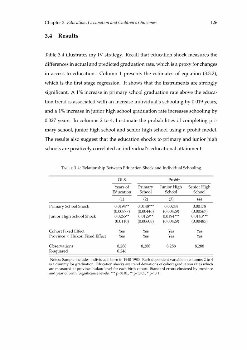
Chapter 3. Education, Occupation and Children’s Outcomes 126
3.4 Results
Table 3.4 illustrates my IV strategy. Recall that education shock measures the
differences in actual and predicted graduation rate, which is a proxy for changes
in access to education. Column 1 presents the estimates of equation (3.3.2),
which is the first stage regression. It shows that the instruments are strongly
significant. A 1% increase in primary school graduation rate above the educa-
tion trend is associated with an increase individual’s schooling by 0.019 years,
and a 1% increase in junior high school graduation rate increases schooling by
0.027 years. In columns 2 to 4, I estimate the probabilities of completing pri-
mary school, junior high school and senior high school using a probit model.
The results also suggest that the education shocks to primary and junior high
schools are positively correlated an individual’s educational attainment.
TABLE 3.4: Relationship Between Education Shock and Individual Schooling
OLS Probit
Years of Primary Junior High Senior HighEducation School School School
(1) (2) (3) (4)
Primary School Shock 0.0194** 0.0148*** 0.00244 0.00178(0.00877) (0.00446) (0.00429) (0.00567)
Junior High School Shock 0.0265** 0.0129** 0.0194*** 0.0143***(0.0110) (0.00608) (0.00429) (0.00485)
Cohort Fixed Effect Yes Yes Yes YesProvince × Hukou Fixed Effect Yes Yes Yes Yes
Observations 8,288 8,288 8,288 8,288R-squared 0.246
Notes: Sample includes individuals born in 1940-1980. Each dependent variable in columns 2 to 4is a dummy for graduation. Education shocks are trend deviations of cohort graduation rates whichare measured at province-hukou level for each birth cohort. Standard errors clustered by provinceand year of birth. Significance levels: *** p<0.01, ** p<0.05, * p<0.1.
Chapter 3. Education, Occupation and Children’s Outcomes 127
3.4.1 First Occupation
The regression results for equation (3.3.1) are presented in Table 3.5. I con-
sider two types of occupational outcomes: non-agricultural job and white-collar
job. Non-agricultural jobs include blue-collar and white-collar occupations. In
columns 1 and 3, the OLS estimates indicate that an additional year of school-
ing increases the probability of obtaining a non-agricultural job by 3.11% and
increases the probability of having a white-collar job by 2.87%. The IV estimates
in columns 2 and 4 suggest a larger effect of schooling on occupational type
(3.81% for non-agricultural job and 3.55% for white-collar job). This finding is
consistent with the existing literature which suggest that the OLS estimates are
biased downwards due to measurement error in schooling.
TABLE 3.5: Impact of Education on First Occupation
Non-Agricultural White CollarOccupation Occupation
OLS IV OLS IV(1) (2) (3) (4)
Years of Education 0.0311*** 0.0381*** 0.0287*** 0.0355***(0.00141) (0.00539) (0.00173) (0.00388)
Cohort Fixed Effect Yes Yes Yes YesProvince × Hukou Fixed Effect Yes Yes Yes Yes
Kleibergen-Paap rk Wald F statistic 16.5 16.5Hansen J statistic 0.049 0.049Observations 8,288 8,288 8,288 8,288
Notes: Sample includes individuals born in 1940-1980. Each dependent variable is a dummy foroccupational outcome. Years of education are instrumented by trend deviations of cohort graduationrates which are measured at province-hukou level for each birth cohort. Standard errors clusteredby province and year of birth. Significance levels: *** p<0.01, ** p<0.05, * p<0.1.
Occupational segregation between rural and urban residents has been a con-
cern in China in the last few decades. The share of urban residents working in
a non-agricultural job or white-collar occupation is much higher than their ru-
ral counterparts; therefore, the impact of schooling on occupational outcomes
is likely to differ across households. To capture this, I estimate equation (3.3.1)
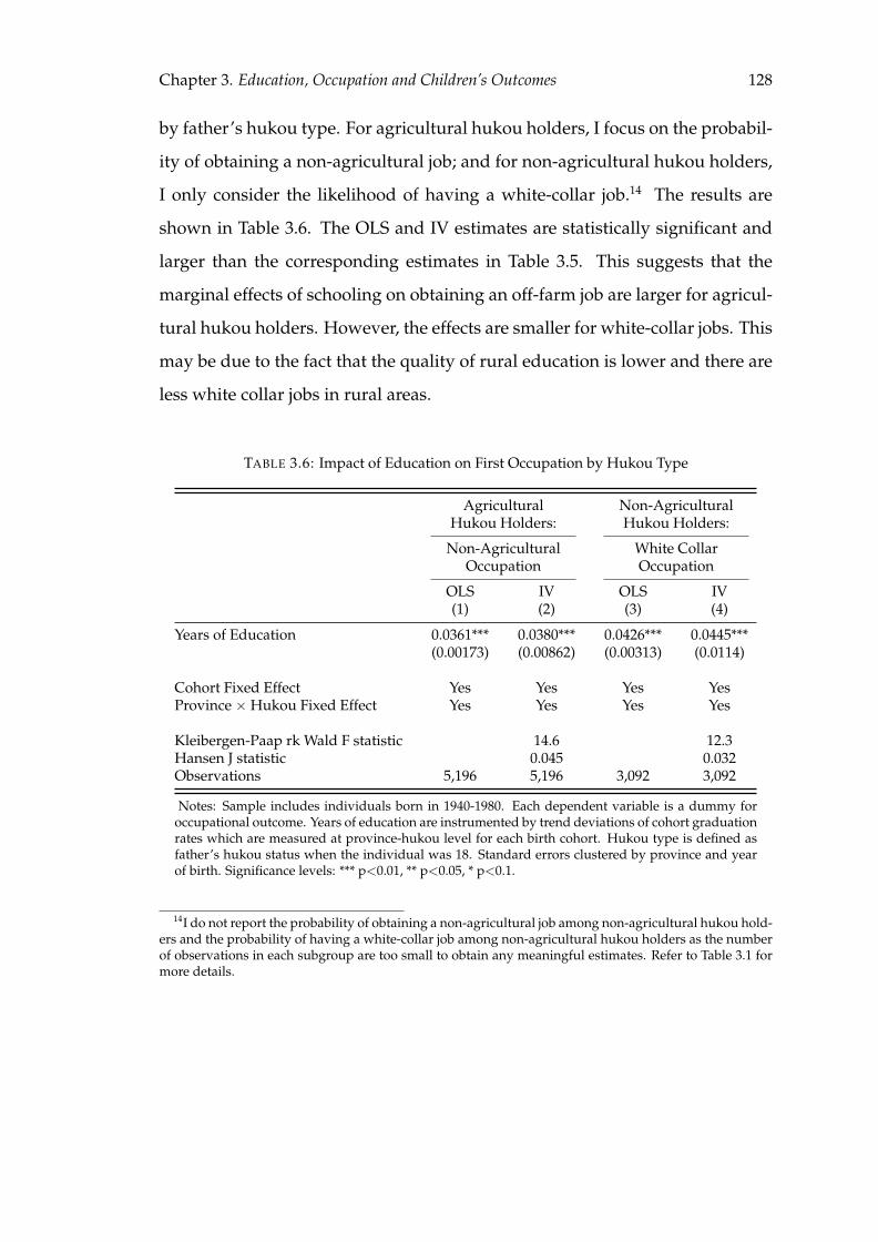
Chapter 3. Education, Occupation and Children’s Outcomes 128
by father’s hukou type. For agricultural hukou holders, I focus on the probabil-
ity of obtaining a non-agricultural job; and for non-agricultural hukou holders,
I only consider the likelihood of having a white-collar job.14 The results are
shown in Table 3.6. The OLS and IV estimates are statistically significant and
larger than the corresponding estimates in Table 3.5. This suggests that the
marginal effects of schooling on obtaining an off-farm job are larger for agricul-
tural hukou holders. However, the effects are smaller for white-collar jobs. This
may be due to the fact that the quality of rural education is lower and there are
less white collar jobs in rural areas.
TABLE 3.6: Impact of Education on First Occupation by Hukou Type
Agricultural Non-AgriculturalHukou Holders: Hukou Holders:
Non-Agricultural White CollarOccupation Occupation
OLS IV OLS IV(1) (2) (3) (4)
Years of Education 0.0361*** 0.0380*** 0.0426*** 0.0445***(0.00173) (0.00862) (0.00313) (0.0114)
Cohort Fixed Effect Yes Yes Yes YesProvince × Hukou Fixed Effect Yes Yes Yes Yes
Kleibergen-Paap rk Wald F statistic 14.6 12.3Hansen J statistic 0.045 0.032Observations 5,196 5,196 3,092 3,092
Notes: Sample includes individuals born in 1940-1980. Each dependent variable is a dummy foroccupational outcome. Years of education are instrumented by trend deviations of cohort graduationrates which are measured at province-hukou level for each birth cohort. Hukou type is defined asfather’s hukou status when the individual was 18. Standard errors clustered by province and yearof birth. Significance levels: *** p<0.01, ** p<0.05, * p<0.1.
14I do not report the probability of obtaining a non-agricultural job among non-agricultural hukou hold-ers and the probability of having a white-collar job among non-agricultural hukou holders as the numberof observations in each subgroup are too small to obtain any meaningful estimates. Refer to Table 3.1 formore details.

Chapter 3. Education, Occupation and Children’s Outcomes 129
3.4.2 Children’s Education
There is a large literature documenting the persistence of educational outcomes
across generations; therefore, one may wonder if increasing parents’ education
also increases children’s educational attainment. To examine the causal rela-
tionship between the two, I estimate equation (3.3.1) for children’s probability
of school completion. I restrict my analysis to individuals born between 1940
and 1960 to ensure that their first child is old enough to complete senior high
school by 2006. 85% of the 1940-60 cohorts reported having at least one child in
2006. As China implemented the compulsory schooling law in 1986, most chil-
dren who were born after 1980 have completed primary education.15 Therefore,
I only consider the likelihood of completing junior high school and senior high
school. Table 3.7 reports the estimation results. It shows that there is a positive
and significant relationship between parent’s and children’s education. The IV
estimates suggest that an additional year of parent’s schooling increases chil-
dren’s probabilities of completing junior high school and senior high school by
3.94% and 4.76% respectively. The OLS estimates are smaller but still positive
and significant.
3.4.3 Discussion and Robustness Checks
There are several caveats in interpreting the results. First, although the educa-
tion reform in 1968-1976 increased the access to basic education, the quality of
education was very poor. As data on teacher’s quality and school curriculum
is unavailable, I cannot control for changes in education quality. Therefore, the
OLS and IV estimates should be interpreted as the lower bound of the impact
of additional years of schooling on occupational and children’s outcomes.15The 1986 compulsory schooling law states that school-aged children are entitled to receive at least
9-years of education. The law was implemented unevenly across regions; therefore, junior high schooldrop-out rates were still quite high during the initial years, especially among the rural households.
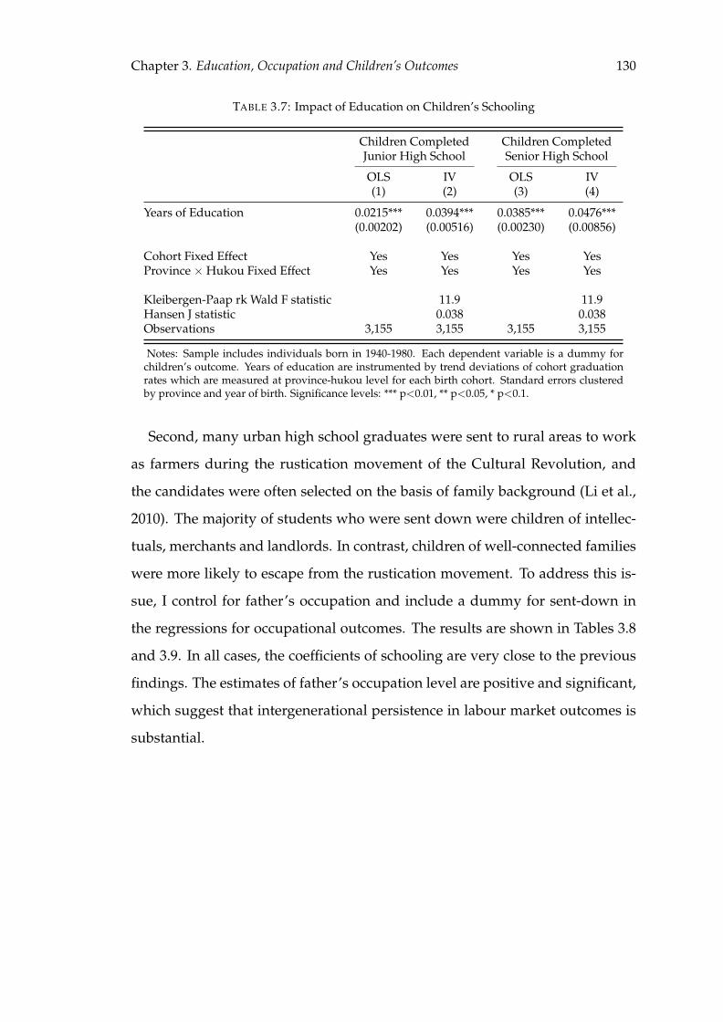
Chapter 3. Education, Occupation and Children’s Outcomes 130
TABLE 3.7: Impact of Education on Children’s Schooling
Children Completed Children CompletedJunior High School Senior High School
OLS IV OLS IV(1) (2) (3) (4)
Years of Education 0.0215*** 0.0394*** 0.0385*** 0.0476***(0.00202) (0.00516) (0.00230) (0.00856)
Cohort Fixed Effect Yes Yes Yes YesProvince × Hukou Fixed Effect Yes Yes Yes Yes
Kleibergen-Paap rk Wald F statistic 11.9 11.9Hansen J statistic 0.038 0.038Observations 3,155 3,155 3,155 3,155
Notes: Sample includes individuals born in 1940-1980. Each dependent variable is a dummy forchildren’s outcome. Years of education are instrumented by trend deviations of cohort graduationrates which are measured at province-hukou level for each birth cohort. Standard errors clusteredby province and year of birth. Significance levels: *** p<0.01, ** p<0.05, * p<0.1.
Second, many urban high school graduates were sent to rural areas to work
as farmers during the rustication movement of the Cultural Revolution, and
the candidates were often selected on the basis of family background (Li et al.,
2010). The majority of students who were sent down were children of intellec-
tuals, merchants and landlords. In contrast, children of well-connected families
were more likely to escape from the rustication movement. To address this is-
sue, I control for father’s occupation and include a dummy for sent-down in
the regressions for occupational outcomes. The results are shown in Tables 3.8
and 3.9. In all cases, the coefficients of schooling are very close to the previous
findings. The estimates of father’s occupation level are positive and significant,
which suggest that intergenerational persistence in labour market outcomes is
substantial.
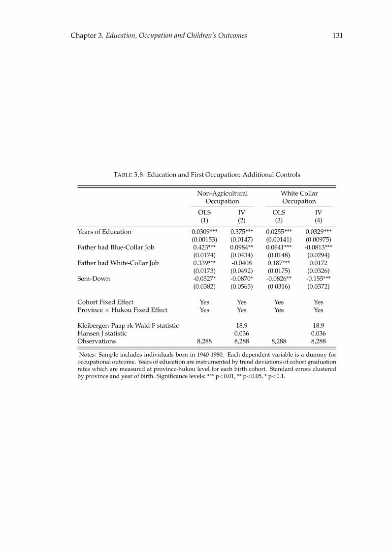
Chapter 3. Education, Occupation and Children’s Outcomes 131
TABLE 3.8: Education and First Occupation: Additional Controls
Non-Agricultural White CollarOccupation Occupation
OLS IV OLS IV(1) (2) (3) (4)
Years of Education 0.0309*** 0.375*** 0.0255*** 0.0329***(0.00153) (0.0147) (0.00141) (0.00975)
Father had Blue-Collar Job 0.423*** 0.0984** 0.0641*** -0.0813***(0.0174) (0.0434) (0.0148) (0.0294)
Father had White-Collar Job 0.339*** -0.0408 0.187*** 0.0172(0.0173) (0.0492) (0.0175) (0.0326)
Sent-Down -0.0527* -0.0870* -0.0826** -0.155***(0.0382) (0.0565) (0.0316) (0.0372)
Cohort Fixed Effect Yes Yes Yes YesProvince × Hukou Fixed Effect Yes Yes Yes Yes
Kleibergen-Paap rk Wald F statistic 18.9 18.9Hansen J statistic 0.036 0.036Observations 8,288 8,288 8,288 8,288
Notes: Sample includes individuals born in 1940-1980. Each dependent variable is a dummy foroccupational outcome. Years of education are instrumented by trend deviations of cohort graduationrates which are measured at province-hukou level for each birth cohort. Standard errors clusteredby province and year of birth. Significance levels: *** p<0.01, ** p<0.05, * p<0.1.
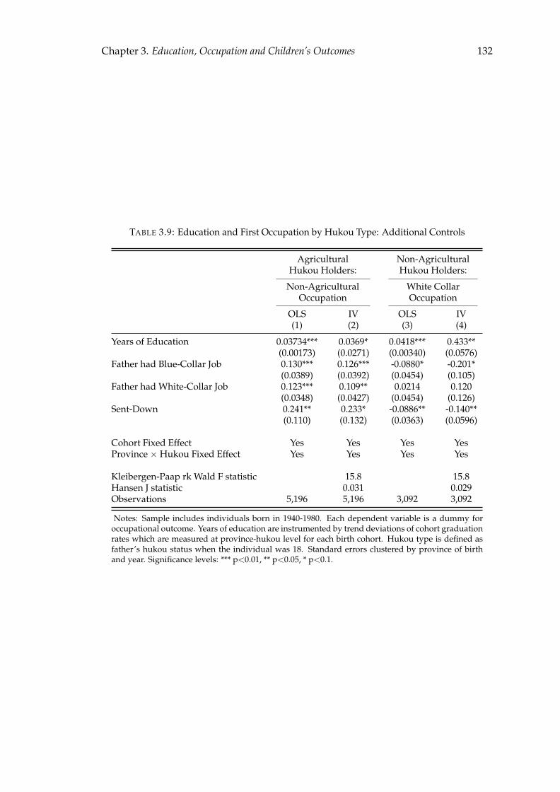
Chapter 3. Education, Occupation and Children’s Outcomes 132
TABLE 3.9: Education and First Occupation by Hukou Type: Additional Controls
Agricultural Non-AgriculturalHukou Holders: Hukou Holders:
Non-Agricultural White CollarOccupation Occupation
OLS IV OLS IV(1) (2) (3) (4)
Years of Education 0.03734*** 0.0369* 0.0418*** 0.433**(0.00173) (0.0271) (0.00340) (0.0576)
Father had Blue-Collar Job 0.130*** 0.126*** -0.0880* -0.201*(0.0389) (0.0392) (0.0454) (0.105)
Father had White-Collar Job 0.123*** 0.109** 0.0214 0.120(0.0348) (0.0427) (0.0454) (0.126)
Sent-Down 0.241** 0.233* -0.0886** -0.140**(0.110) (0.132) (0.0363) (0.0596)
Cohort Fixed Effect Yes Yes Yes YesProvince × Hukou Fixed Effect Yes Yes Yes Yes
Kleibergen-Paap rk Wald F statistic 15.8 15.8Hansen J statistic 0.031 0.029Observations 5,196 5,196 3,092 3,092
Notes: Sample includes individuals born in 1940-1980. Each dependent variable is a dummy foroccupational outcome. Years of education are instrumented by trend deviations of cohort graduationrates which are measured at province-hukou level for each birth cohort. Hukou type is defined asfather’s hukou status when the individual was 18. Standard errors clustered by province of birthand year. Significance levels: *** p<0.01, ** p<0.05, * p<0.1.

Chapter 3. Education, Occupation and Children’s Outcomes 133
As discussed earlier, my measure of education shock relies on the assump-
tion that there is no change in hukou status before the time of survey. If the
probability of hukou switching is correlated with some regional factors which
affect individual’s occupation or children’s schooling, my instruments would
be endogenous and the IV estimates are biased. To tackle this problem, I esti-
mate equations (3.3.1) on the basis of the 1% sample of 1990 population census.
The main advantage of using the 1990 census is migration and hukou switching
were strongly restricted before the mid-1990s, therefore the number of hukou
switchers was much lower in 1990. However, I am forced to restrict my anal-
ysis to a smaller sample which excludes individuals born between 1971 and
1980. Appendix Figure 3.6 plots the histograms of the new estimates of educa-
tion shocks. It shows that the distributions of education shocks based on the
1990 and 2000 census are very similar. In Appendix Tables 3.11-3.14, I present
the regression results of equations (3.3.1) using the 1990 census-based education
shocks as instruments for schooling. The results are robust to the new measures,
which suggest that hukou switching is not a serious issue.
At last, my second stage estimation is based on a linear probability model.
The advantage of this approach is that the magnitude of effects are easy to in-
terpret. However, the linear least square method has an implicit assumption
that the dependent variable is continuous and can take values other than zero
and one. I re-estimate the second stage using a probit model and still find pos-
itive and significant effects of schooling on occupational status and children’s
educational performance. The results are shown in Appendix Tables 3.15-3.17 .
3.5 Conclusion
This paper studies the impact of education on occupational status and chil-
dren’s educational attainment. To tackle the problem of endogenous schooling,
I use the education shock during the Cultural Revolution as an instrument for

Chapter 3. Education, Occupation and Children’s Outcomes 134
individual’s schooling. The education reform in 1968-76 improved the access to
basic education, which led to a significant growth in primary school and junior
high school graduation rates for cohorts born in 1950-65. The trend deviations
in primary school and junior school graduation rates are exogenous to other fac-
tors that are correlated with the individual’s future outcomes. The estimation
results show that increase in years of schooling leads to better occupational and
children’s outcomes. This finding suggest that public investment in education
plays an important role in social mobility within and across generations.
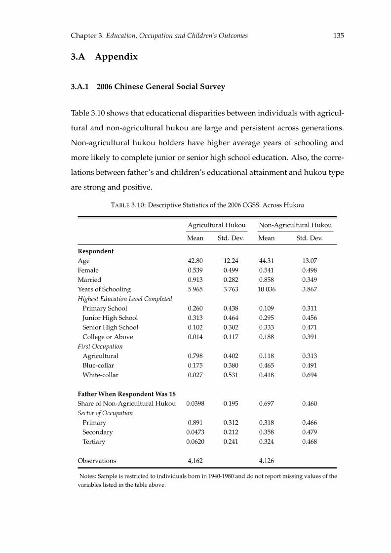
Chapter 3. Education, Occupation and Children’s Outcomes 135
3.A Appendix
3.A.1 2006 Chinese General Social Survey
Table 3.10 shows that educational disparities between individuals with agricul-
tural and non-agricultural hukou are large and persistent across generations.
Non-agricultural hukou holders have higher average years of schooling and
more likely to complete junior or senior high school education. Also, the corre-
lations between father’s and children’s educational attainment and hukou type
are strong and positive.
TABLE 3.10: Descriptive Statistics of the 2006 CGSS: Across Hukou
Agricultural Hukou Non-Agricultural Hukou
Mean Std. Dev. Mean Std. Dev.
RespondentAge 42.80 12.24 44.31 13.07Female 0.539 0.499 0.541 0.498Married 0.913 0.282 0.858 0.349Years of Schooling 5.965 3.763 10.036 3.867Highest Education Level Completed
Primary School 0.260 0.438 0.109 0.311Junior High School 0.313 0.464 0.295 0.456Senior High School 0.102 0.302 0.333 0.471College or Above 0.014 0.117 0.188 0.391
First OccupationAgricultural 0.798 0.402 0.118 0.313Blue-collar 0.175 0.380 0.465 0.491White-collar 0.027 0.531 0.418 0.694
Father When Respondent Was 18Share of Non-Agricultural Hukou 0.0398 0.195 0.697 0.460Sector of Occupation
Primary 0.891 0.312 0.318 0.466Secondary 0.0473 0.212 0.358 0.479Tertiary 0.0620 0.241 0.324 0.468
Observations 4,162 4,126
Notes: Sample is restricted to individuals born in 1940-1980 and do not report missing values of thevariables listed in the table above.
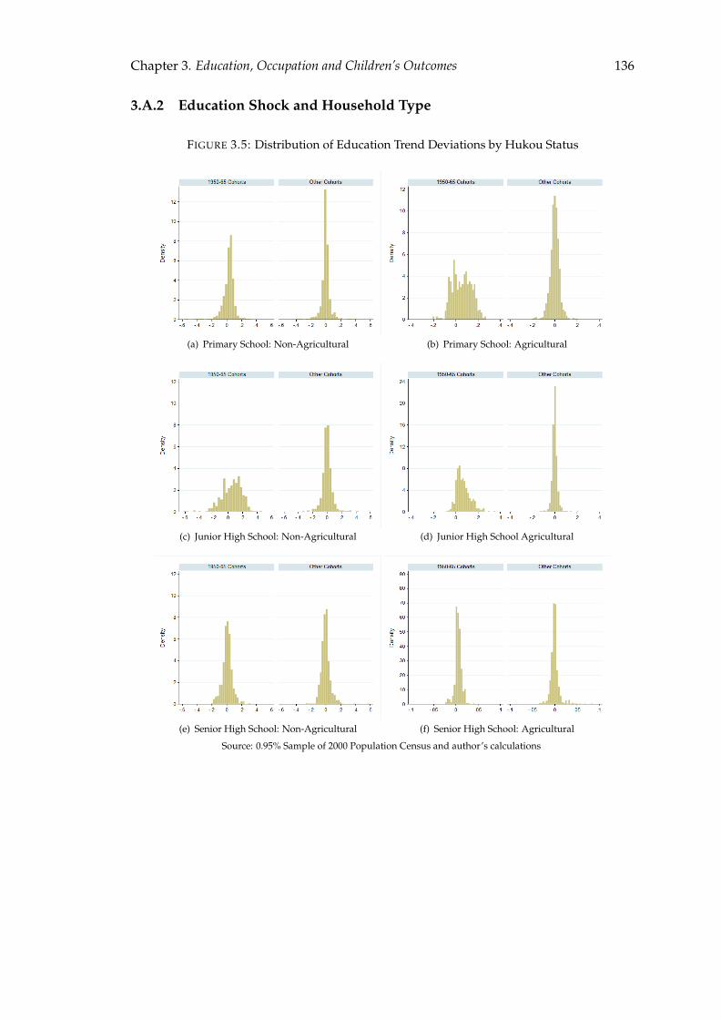
Chapter 3. Education, Occupation and Children’s Outcomes 136
3.A.2 Education Shock and Household Type
FIGURE 3.5: Distribution of Education Trend Deviations by Hukou Status
(a) Primary School: Non-Agricultural (b) Primary School: Agricultural
(c) Junior High School: Non-Agricultural (d) Junior High School Agricultural
(e) Senior High School: Non-Agricultural (f) Senior High School: Agricultural
Source: 0.95% Sample of 2000 Population Census and author’s calculations
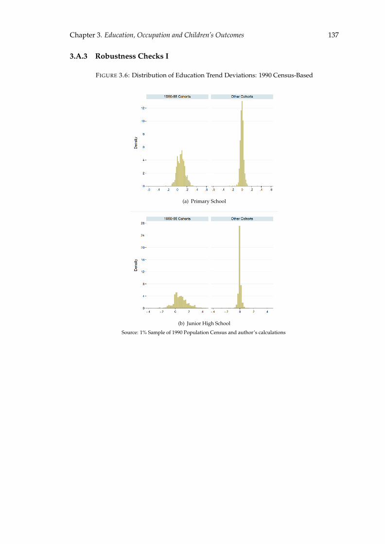
Chapter 3. Education, Occupation and Children’s Outcomes 137
3.A.3 Robustness Checks I
FIGURE 3.6: Distribution of Education Trend Deviations: 1990 Census-Based
(a) Primary School
(b) Junior High School
Source: 1% Sample of 1990 Population Census and author’s calculations
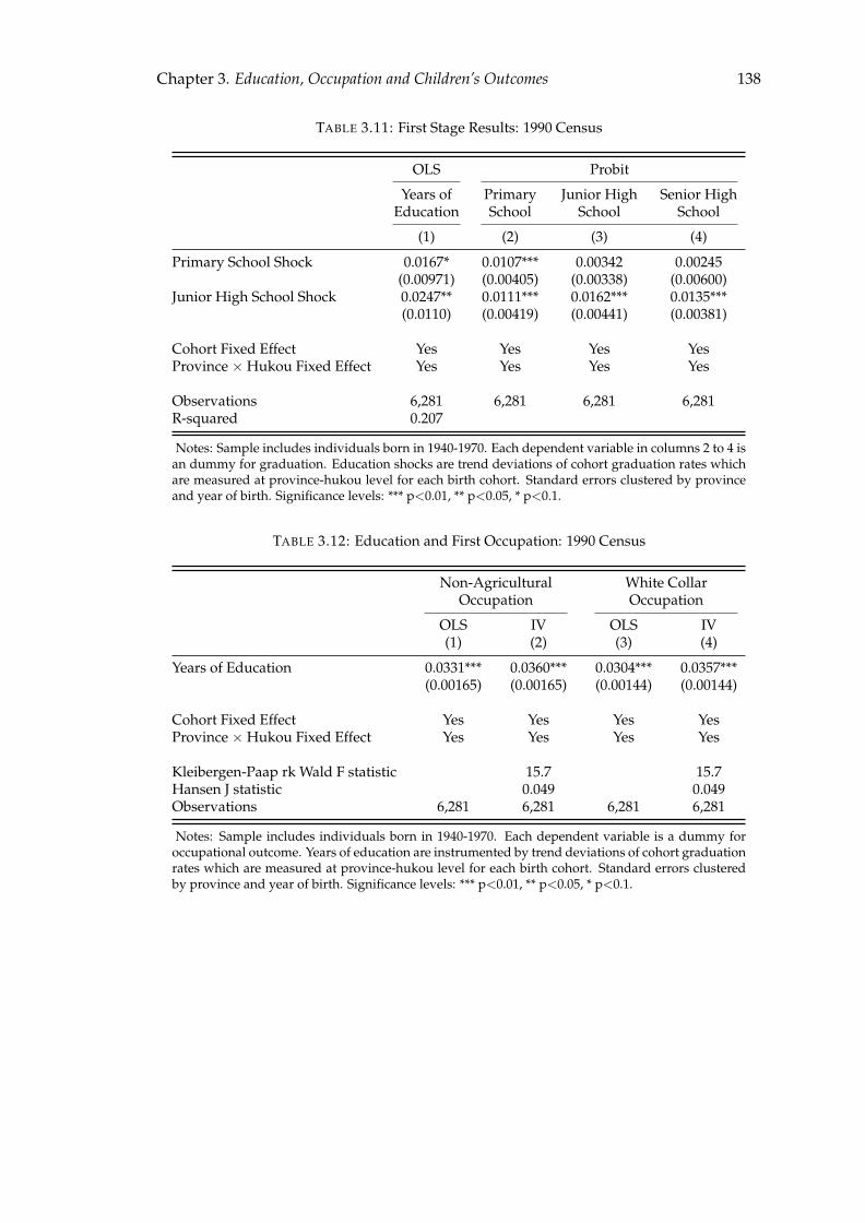
Chapter 3. Education, Occupation and Children’s Outcomes 138
TABLE 3.11: First Stage Results: 1990 Census
OLS Probit
Years of Primary Junior High Senior HighEducation School School School
(1) (2) (3) (4)
Primary School Shock 0.0167* 0.0107*** 0.00342 0.00245(0.00971) (0.00405) (0.00338) (0.00600)
Junior High School Shock 0.0247** 0.0111*** 0.0162*** 0.0135***(0.0110) (0.00419) (0.00441) (0.00381)
Cohort Fixed Effect Yes Yes Yes YesProvince × Hukou Fixed Effect Yes Yes Yes Yes
Observations 6,281 6,281 6,281 6,281R-squared 0.207
Notes: Sample includes individuals born in 1940-1970. Each dependent variable in columns 2 to 4 isan dummy for graduation. Education shocks are trend deviations of cohort graduation rates whichare measured at province-hukou level for each birth cohort. Standard errors clustered by provinceand year of birth. Significance levels: *** p<0.01, ** p<0.05, * p<0.1.
TABLE 3.12: Education and First Occupation: 1990 Census
Non-Agricultural White CollarOccupation Occupation
OLS IV OLS IV(1) (2) (3) (4)
Years of Education 0.0331*** 0.0360*** 0.0304*** 0.0357***(0.00165) (0.00165) (0.00144) (0.00144)
Cohort Fixed Effect Yes Yes Yes YesProvince × Hukou Fixed Effect Yes Yes Yes Yes
Kleibergen-Paap rk Wald F statistic 15.7 15.7Hansen J statistic 0.049 0.049Observations 6,281 6,281 6,281 6,281
Notes: Sample includes individuals born in 1940-1970. Each dependent variable is a dummy foroccupational outcome. Years of education are instrumented by trend deviations of cohort graduationrates which are measured at province-hukou level for each birth cohort. Standard errors clusteredby province and year of birth. Significance levels: *** p<0.01, ** p<0.05, * p<0.1.
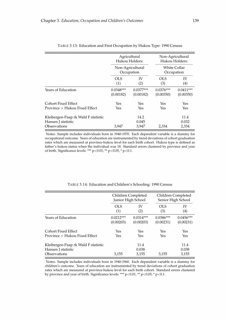
Chapter 3. Education, Occupation and Children’s Outcomes 139
TABLE 3.13: Education and First Occupation by Hukou Type: 1990 Census
Agricultural Non-AgriculturalHukou Holders: Hukou Holders:
Non-Agricultural White CollarOccupation Occupation
OLS IV OLS IV(1) (2) (3) (4)
Years of Education 0.0348*** 0.0377*** 0.0376*** 0.0411***(0.00182) (0.00182) (0.00350) (0.00350)
Cohort Fixed Effect Yes Yes Yes YesProvince × Hukou Fixed Effect Yes Yes Yes Yes
Kleibergen-Paap rk Wald F statistic 14.2 11.4Hansen J statistic 0.045 0.032Observations 3,947 3,947 2,334 2,334
Notes: Sample includes individuals born in 1940-1970. Each dependent variable is a dummy foroccupational outcome. Years of education are instrumented by trend deviations of cohort graduationrates which are measured at province-hukou level for each birth cohort. Hukou type is defined asfather’s hukou status when the individual was 18. Standard errors clustered by province and yearof birth. Significance levels: *** p<0.01, ** p<0.05, * p<0.1.
TABLE 3.14: Education and Children’s Schooling: 1990 Census
Children Completed Children CompletedJunior High School Senior High School
OLS IV OLS IV(1) (2) (3) (4)
Years of Education 0.0212*** 0.0314*** 0.0386*** 0.0456***(0.00203) (0.00203) (0.00231) (0.00231)
Cohort Fixed Effect Yes Yes Yes YesProvince × Hukou Fixed Effect Yes Yes Yes Yes
Kleibergen-Paap rk Wald F statistic 11.4 11.4Hansen J statistic 0.038 0.038Observations 3,155 3,155 3,155 3,155
Notes: Sample includes individuals born in 1940-1960. Each dependent variable is a dummy forchildren’s outcome. Years of education are instrumented by trend deviations of cohort graduationrates which are measured at province-hukou level for each birth cohort. Standard errors clusteredby province and year of birth. Significance levels: *** p<0.01, ** p<0.05, * p<0.1.
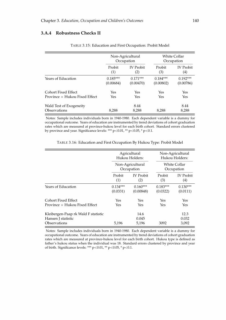
Chapter 3. Education, Occupation and Children’s Outcomes 140
3.A.4 Robustness Checks II
TABLE 3.15: Education and First Occupation: Probit Model
Non-Agricultural White CollarOccupation Occupation
Probit IV Probit Probit IV Probit(1) (2) (3) (4)
Years of Education 0.185*** 0.171*** 0.184*** 0.192***(0.00684) (0.00470) (0.00802) (0.00786)
Cohort Fixed Effect Yes Yes Yes YesProvince × Hukou Fixed Effect Yes Yes Yes Yes
Wald Test of Exogeneity 8.44 8.44Observations 8,288 8,288 8,288 8,288
Notes: Sample includes individuals born in 1940-1980. Each dependent variable is a dummy foroccupational outcome. Years of education are instrumented by trend deviations of cohort graduationrates which are measured at province-hukou level for each birth cohort. Standard errors clusteredby province and year. Significance levels: *** p<0.01, ** p<0.05, * p<0.1.
TABLE 3.16: Education and First Occupation By Hukou Type: Probit Model
Agricultural Non-AgriculturalHukou Holders: Hukou Holders:
Non-Agricultural White CollarOccupation Occupation
Probit IV Probit Probit IV Probit(1) (2) (3) (4)
Years of Education 0.134*** 0.160*** 0.183*** 0.130***(0.0331) (0.00848) (0.0322) (0.0111)
Cohort Fixed Effect Yes Yes Yes YesProvince × Hukou Fixed Effect Yes Yes Yes Yes
Kleibergen-Paap rk Wald F statistic 14.6 12.3Hansen J statistic 0.045 0.032Observations 5,196 5,196 3092 3,092
Notes: Sample includes individuals born in 1940-1980. Each dependent variable is a dummy foroccupational outcome. Years of education are instrumented by trend deviations of cohort graduationrates which are measured at province-hukou level for each birth cohort. Hukou type is defined asfather’s hukou status when the individual was 18. Standard errors clustered by province and yearof birth. Significance levels: *** p<0.01, ** p<0.05, * p<0.1.

Chapter 3. Education, Occupation and Children’s Outcomes 141
TABLE 3.17: Education and Children’s Schooling: Probit Model
Children Completed Children CompletedJunior High School Senior High School
Probit IV Probit Probit IV Probit(1) (2) (3) (4)
Years of Education 0.0843*** 0.169*** 0.110*** 0.237***(0.00858) (0.0203) (0.00751) (0.0104)
Cohort Fixed Effect Yes Yes Yes YesProvince × Hukou Fixed Effect Yes Yes Yes Yes
Wald Test of Exogeneity 5.18 5.18Observations 3,155 3,155 3,155 3,155
Notes: Sample includes individuals born in 1940-1960. Each dependent variable is a dummy forchildren’s outcome. Years of education are instrumented by trend deviations of cohort graduationrates which are measured at province-hukou level for each birth cohort. Standard errors clusteredby province and year of birth. Significance levels: *** p<0.01, ** p<0.05, * p<0.1.
Bibliography
Abowd, J. M., J. Haltiwanger, R. Jarmin, J. Lane, P. Lengermann, K. McCue,
K. McKinney, and K. Sandusky (2005, December). The Relation among Hu-
man Capital, Productivity, and Market Value: Building Up from Micro Evi-
dence. In Measuring Capital in the New Economy, NBER Chapters, pp. 153–204.
National Bureau of Economic Research.
Abowd, J. M., F. Kramarz, and D. N. Margolis (1999). High Wage Workers and
High Wage Firms. Econometrica 67(2), pp. 251–333.
Abramovitz, M. (1956). Resource and Output Trends in the United States Since
1870. American Economic Review, 5–23.
Afridi, F., S. Li, and Y. Ren (2012). Social Identity and Inequality: The Impact of
China’s Hukou System. Working Paper.
Aghion, P., R. Burgess, S. Redding, and F. Zilibotti (2008). The Unequal Effects of
Liberalization: Evidence from Dismantling the License Raj in India. American
Economic Review 98(4), 1397–1412.
Amiti, M. and D. R. Davis (2012). Trade, Firms and Wages: Theory and Evi-
dence. Review of Economic Studies 79(1), 1–36.
Amiti, M. and J. Konings (2007). Trade Liberalization, Intermediate Inputs,
and Productivity: Evidence from Indonesia. American Economic Review 97(5),
1611–1635.
Atalay, E., A. Hortacsu, and C. Syverson (2012). Why Do Firms Own Production
Chains? NBER Working Paper No. 18020.
142
Bibliography 143
Bandiera, O., I. Barankay, and I. Rasul (2009). Social Connections and Incen-
tives in the Workplace: Evidence from Personnel Data. Econometrica 77(4),
pp. 1047–1094.
Bas, M. and V. Strauss-Kahn (2012). Trade Liberalization and Export Prices: The
Case of China. Working Paper.
Baum-Snow, N., L. Brandt, J. V. Henderson, M. A. Turner, and Q. Zhang (2012).
Roads,RailroadsandDecentralizationofChineseCities. Working Paper.
Becker, G. S. (1962). Investment in Human Capital: A Theoretical Analysis.
Journal of Political Economy 70(5), 9–49.
Becker, G. S. and N. Tomes (1986). Human Capital and the Rise and Fall of
Families. Journal of Labor Economics 4(3), 1–39.
Bernard, A., S. Redding, and P. Schott (2007). Comparative Advantage and
Heterogeneous Firms. Review of Economic Studies 74(1), 31–66.
Bernard, A. B., S. Redding, and P. K. Schott (2010). Multiple-product Firms and
Product Switching. American Economic Review 100(1), 70–97.
Bernhofen, D. M. and J. C. Brown (2011). Testing the General Validity of the
Heckscher-Ohlin Theorem: The Natural Experiment of Japan. CESifo Working
Paper Series 3586.
Bernstein, J. R. and D. E. Weinstein (2002). Do Endowments Predict the Location
of Production? Evidence from National and International data. Journal of
International Economics 56(1), 55–76.
Bilbiie, F., F. Ghironi, and M. J. Melitz (2012). Endogenous Entry, Product Vari-
ety, and Business Cycles. Journal of Political Economy 120(2), 304–345.
Birdsall, N. (1985). Public Inputs and Children Schooling in Brazil. Journal of
Development Economics 18, 67–68.
Bibliography 144
Black, S. E., P. J. Devereux, and K. G. Salvanes (2005). Why the Apple Doesn’t
Fall Far: Understanding Intergenerational Transmission of Human Capital.
American Economic Review 95(1), 437–449.
Bloom, N., M. Schankerman, and J. van Reenen (2007). Identifying Technology
Spillovers and Product Market Rivalry. NBER Working Paper No. 13060.
Bloom, N. and J. van Reenen (2007). Measuring and Explaining Management
Practices across Firms and Countries. Quarterly Journal of Economics 122(4),
1351–1408.
Bombardini, M., G. Gallipoli, and G. Pupato (2012). Skill Dispersion and Trade
Flows. American Economic Review 102(5), 2327–48.
Borjas, G. (2009). The Analytics of the Wage Effect of Immigration. Working
Paper.
Borjas, G. J. (2003). The Labor Demand Curve Is Downward Sloping: Reexam-
ining The Impact Of Immigration On The Labor Market. Quarterly Journal of
Economics 118(4), 1335–1374.
Bowles, S. (1970). Aggregation of Labor Inputs in the Economics of Growth and
Planning: Experiments with a Two-Level CES Function. Journal of Political
Economy 78(1), 68–81.
Brandt, L., J. V. Biesebroeck, and Y. Zhang (2012). Creative Accounting or Cre-
ative Destruction? Firm-Level Productivity Growth in Chinese Manufactur-
ing. Journal of Development Economics 97(2), 339–351.
Chan, K. W. and W. Buckingham (2008). Is China Abolishing the Hukou Sys-
tem? The China Quarterly 195, 582–606.
Chan, K. W., T. Liu, and Y. Yang (1999). Hukou and Non-hukou Migrations in
China: Comparisons and Contrasts. International Journal of Population Geogra-
phy 5, 425–448.
Bibliography 145
Chow, G. C. (1993). Capital Formation and Economic Growth in China. The
Quarterly Journal of Economics 108, 809–842.
Defever, F. and A. Riano (2012). Pure-Exporter Subsidies: The Non-Reform of
China’s Trade Policy. Working Paper.
Duflo, E. (2001). Schooling and Labor Market Consequences of School Con-
struction in Indonesia: Evidence from an Unusual Policy Experiment. Ameri-
can Economic Review 91(4), 795–813.
Faber, B. (2012). Trade Integration, Market Size, And Industrialization: Evi-
dence From China’s National Trunk Highway System. Working Paper.
Fitzgerald, D. and J. C. Hallak (2004). Specialization, Factor Accumulation and
Development. Journal of International Economics 64(2), 277–302.
Fleisher, B. M. and X. Wang (2004). Skill Differentials, Return to Schooling, and
Market Segmentation in a Transition Economy: the Case of Mainland China.
Journal of Development Economics 73(1), 315–328.
Fox, J. T. and V. Smeets (2011). Does Input Quality Drive Measured Differences
in Firm Productivity? NBER Working Paper No. 16853 (16853).
Garicano, L. and P. Heaton (2010). Information Technology, Organization, and
Productivity in the Public Sector: Evidence from Police Departments. Journal
of Labor Economics 28(1), 167–201.
Giles, J., A. Park, and M. Wang (2008). The Great Proletarian Cultural Revolu-
tion, Disruptions to Education, and Returns to Schooling in Urban China. The
World Bank Policy Research Working Paper 4729.
Goldberg, P. K., A. Khandelwal, N. Pavcnik, and P. Topalova (2010). Imported
Intermediate Inputs and Domestic Product Growth: Evidence from India.
Quarterly Journal of Economics 125(4), 1727–1767.
Bibliography 146
Goldberg, P. K. and N. Pavcnik (2005). Trade, Wages and the Political Econ-
omy of Trade Protection: Evidence from Colombian Trade Reforms. Journal of
International Economics 66(1), 75–105.
Grossman, G. M. and G. Maggi (2000). Diversity and Trade. American Economic
Review 90(5), 1255–1275.
Helpman, E., O. Itskhoki, and S. Redding (2010a). Inequality and Unemploy-
ment in a Global Economy. Econometrica 78(4), 1239–1283.
Helpman, E., O. Itskhoki, and S. Redding (2010b). Unequal Effects of Trade on
Workers with Different Abilities. Journal of the European Economic Association
Papers & Proceedings 8(2-3), 421–433.
Hirschman, A. (1958). The Strategy of Economic Development. Encore Edition
Series. Westview Press.
Holmlund, H. (2008). Intergenerational Mobility and Assortative Mating: Ef-
fects of an Educational Reform. CEE Discussion Papers 0091.
Horta, A. and C. Syverson (2007). Cementing Relationships: Vertical Integra-
tion, Foreclosure, Productivity, and Prices. Journal of Political Economy 115(2),
250–301.
Hsieh, C.-T. and P. J. Klenow (2009). Misallocation and Manufacturing TFP in
China and India. Quarterly Journal of Economics 124(4), 1403–1448.
Ilmakunnas, P. and S. Ilmakunnas (2011). Diversity at the Workplace: Whom
Does it Benefit? De Economist 159(2), 223–255.
Iranzo, S., F. Schivardi, and E. Tosetti (2008). Skill Dispersion and Firm Produc-
tivity: An Analysis with Employer-Employee Matched Data. Journal of Labor
Economics 26(2), 247–285.
Javorcik, B. S. (2004). Does Foreign Direct Investment Increase the Productiv-
ity of Domestic Firms? In Search of Spillovers Through Backward Linkages.
American Economic Review 94(3), 605–627.
Bibliography 147
Karadi, P. and M. Koren (2012). Cattle, Steaks and Restaurants: Development
Accounting when Space Matters. Working Paper.
Kennan, J. and J. R. Walker (2011). The Effect of Expected Income on Individual
Migration Decisions. Econometrica 79(1), 211–251.
Kugler, M. and E. Verhoogen (2011). Prices, Plant Size, and Product Quality.
Review of Economic Studies 79(1), 307–339.
Lavy, V. (1996). School Supply Constraints and Children’s Educational Out-
comes in Rural Ghana. Journal of Development Economics 51, 291–314.
Lazear, E. P. (2000). Performance Pay and Productivity. The American Economic
Review 90(5), pp. 1346–1361.
Lewis, W. (1954). Economic Development with Unlimited Supplies of Labour.
The Manchester School 22(2), 139–191.
Li, H., M. Rosenzweig, and J. Zhang (2010). Altruism, Favoritism, and Guilt
in the Allocation of Family Resources: Sophie’s Choice in Mao’s Mass Send
Down Movement. Journal of Political Economy 118(1), 1–38.
Ma, Y., H. Tang, and Y. Zhang (2012). Factor Intensity, Product Switching, and
Productivity: Evidence from Chinese Exporters. Working Paper.
Manova, K. and Z. Zhang (2012). Export Prices Across Firms and Destinations.
Quarterly Journal of Economics 127(1), 379–436.
Martins, P. S. (2008). Dispersion in Wage Premiums and Firm Performance.
Economics Letters 101, 63–65.
Maurin, E. and S. McNally (2008). Vive la Rlution! Long Term Returns of 1968
to the Angry Students. Journal of Labor Economics 26(1), 1–33.
Melitz, M. J. (2003). The Impact of Trade on Intra-industry Reallocations and
Aggregate Industry Productivity. Econometrica 71(6), 1695–1725.
Bibliography 148
Melitz, M. J. and G. I. P. Ottaviano (2008). Market Size, Trade, and Productivity.
Review of Economic Studies 75(1), 295–316.
Meng, X. and B. Gregory (2007). Exploring the Impact of Interrupted Education
on Earnings: The Educational Cost of the Chinese Cultural Revolution. IZA
Discussion Paper No. 2548.
Moretti, E. (2004). Workers’ Education, Spillovers, and Productivity: Evidence
from Plant-Level Production Functions. American Economic Review 94(3), 656–
690.
Moretti, E. (2011). Chapter 14 - Local Labor Markets. In Handbook of Labor
Economics, Volume 4, Part B, pp. 1237 – 1313. Elsevier.
Morrow, J. (2010). Is Skill Disperison a Source of Productivity and Exports in
Developing Countries? Working Paper.
Oreopoulos, P., M. E. Page, and A. H. Stevens (2006). The Intergenerational
Effects of Compulsory Schooling. Journal of Labor Economics 26, 455–483.
Ottaviano, G. and G. Peri (2010). Rethinking the Effect of Immigration on
Wages. Working Paper.
Overman, H. G. and D. Puga (2010). Labor Pooling as a Source of Agglomer-
ation: An Empirical Investigation. In Agglomeration Economics, NBER Chap-
ters, pp. 133–150. National Bureau of Economic Research, Inc.
Ozyurt, S. (2009). Total Factor Productivity Growth in Chinese Industry: 1952-
2005. Oxford Development Studies 37(1), 1–17.
Parrotta, P., D. Pozzoli, and M. Pytlikova (2011). Does Labor Diversity affect
Firm Productivity? Norface Migration Discussion Paper No. 2011-22.
Pekkarinen, T., R. Uusitalo, and S. Pekkala (2006). Education Policy and In-
tergenerational Income Mobility: Evidence from the Finnish Comprehensive
School Reform. IZA Discussion Paper No. 2204.
Bibliography 149
Syverson, C. (2004). Market Structure and Productivity: A Concrete Example.
Journal of Political Economy 112(6), 1181–1222.
Syverson, C. (2011). What Determines Productivity? Journal of Economic Litera-
ture 49(2), 326–365.
Topalova, P. (2010). Factor Immobility and Regional Impacts of Trade Liberal-
ization: Evidence on Poverty from India. American Economic Journal: Applied
Economics 2(4), 1–41.
Trefler, D. (1993). Trade Liberalization and the Theory of Endogenous Protec-
tion: An Econometric Study of U.S. Import Policy. Journal of Political Econ-
omy 101(1), 138–160.
Trefler, D. (1994). Protection, Trade, and Wages: Evidence from U.S. Manufac-
turing. Industrial and Labor Relations Review 47(4), 574–593.
Trefler, D. (2004). The Long and Short of the Canada-U.S. Free Trade Agreement.
American Economic Review 94(4), 870–895.
Vanek, J. (1968). The Factor Proportions Theory: The N-Factor Case. Kyk-
los 21(4), 749–756.
Verhoogen, E. A. (2008). Trade, Quality Upgrading and Wage Inequality in the
Mexican Manufacturing Sector. Quarterly Journal of Economics 123(2), 489–530.
Yu, M. (2011). Processing Trade, Tarff Reductions, and Firm Productivity: Evi-
dence from Chinese Products. CCER Working Paper.


![Three Brief Essays Concerning Chinese · PDF fileThree Brief Essays Concerning Chinese Tocharistan ... and cantos (quzi[ci]), transformation texts ... subsequent ostensible disappearance](https://img.pdfslide.net/doc/110x75/5a8c0bb17f8b9ac87a8cf465/three-brief-essays-concerning-chinese-brief-essays-concerning-chinese-tocharistan.jpg)