Embed Size (px)
Citation preview
AN ABSTRACT OF THE THESIS OF
CHIA -CHENG KING for the M. S. in Electrical Engineering (Name) (Degree)
Date thesis is presented
(Major)
Title DIGITAL COMPUTER ANALYSIS AND SYNTHESIS OF
LINEAR FEEDBACK CONTROL SYSTEMS USING
SUPERPOSITION INTEGRALS
Abstract approved (Major professor)
Theoretical bases and techniques are discussed in this
paper for practical numerical analysis and synthesis of linear
feedback control systems. Criterion are based on the super-
position integrals.
A synthesis method is introduced to find the impulse re-
sponse of a system or a part of the system. The existing system
can be analyzed by using these impulse responses for unity or
non -unity feedback systems.
A method for compensation of an existing system is also
introduced, and the transfer function of the required compensating
network can be computed directly from its computed impulse
function.
p.,,p /gß /963

Several examples for each kind of problem have been
computed by using IBM 1620. Information of how to determine
the required time increment is given to assure computation ac-
curacy.
DIGITAL COMPUTER ANALYSIS AND SYNTHESIS OF LINEAR FEEDBACK CONTROL SYSTEMS USING
SUPERPOSITION INTEGRALS
by
CHIA -CHENG KING
A THESIS
submitted to
OREGON STATE UNIVERSITY
in partial fulfillment of the requirements for the
degree of
MASTER OF SCIENCE
August 1963
APPROVED:
Assistant Professor of Electrical Engineering
In Charge of Major
Heed of Departmen of Electrical Engineering
Dean of Graduate School
Date thesis is presented ä
/8), 963
Typed by Jolene Hunter Wuest

ACKNOWLEDGMENT
The writer is greatly indebted to Professor Solon A. Stone
for his valuable help and comments in the preparation of the manu-
script.
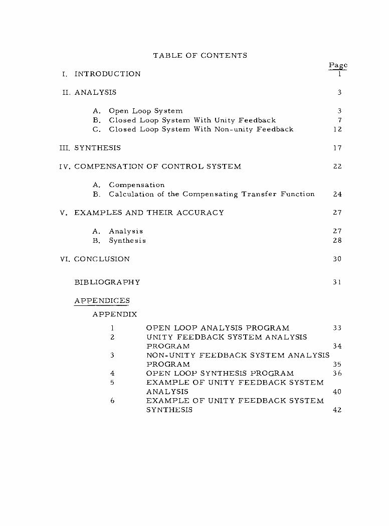
TABLE OF CONTENTS Page
I. INTRODUCTION 1
II. ANALYSIS 3
A. Open Loop System 3
B. Closed Loop System With Unity Feedback 7
C. Closed Loop System With Non -unity Feedback 12
III. SYNTHESIS 17
IV. COMPENSATION OF CONTROL SYSTEM 22
A. Compensation B. Calculation of the Compensating Transfer Function 24
V. EXAMPLES AND THEIR ACCURACY 27
A. Analysis 27 B. Synthesis 28
VI. CONCLUSION 30
BIBLIOGRAPHY 31
APPENDICES
APPENDIX
1 OPEN LOOP ANALYSIS PROGRAM 2 UNITY FEEDBACK SYSTEM ANALYSIS
PROGRAM 3 NON -UNITY FEEDBACK SYSTEM ANALYSIS
PROGRAM 4 OPEN LOOP SYNTHESIS PROGRAM 5 EXAMPLE OF UNITY FEEDBACK SYSTEM
ANALYSIS 6 EXAMPLE OF UNITY FEEDBACK SYSTEM
SYNTHESIS
33
34
35 36
40
42
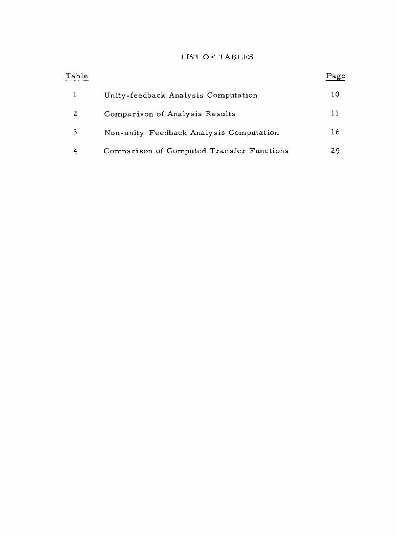
LIST OF TABLES
Table Page
1 Unity- feedback Analysis Computation 10
2 Comparison of Analysis Results 11
3 Non -unity Feedback Analysis Computation 16
4 Comparison of Computed Transfer Functions 29
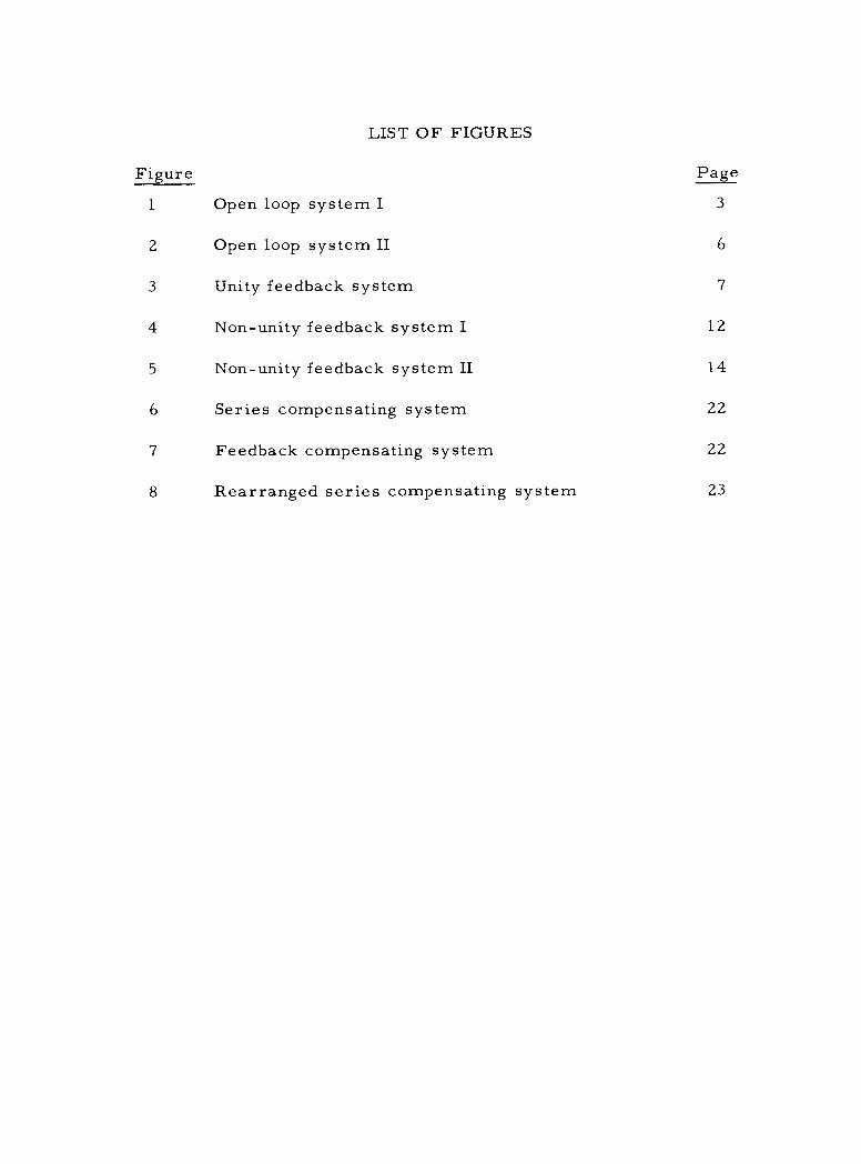
LIST OF FIGURES
Figure Page
1 Open loop system I 3
2 Open loop system II 6
3 Unity feedback system 7
4 Non -unity feedback system I 12
5 Non -unity feedback system II 14
6 Series compensating system 22
7 Feedback compensating system 22
8 Rearranged series compensating system 23
DIGITAL COMPUTER ANALYSIS AND SYNTHESIS OF LINEAR FEEDBACK CONTROL SYSTEMS USING
SUPERPOSITION INTEGRALS
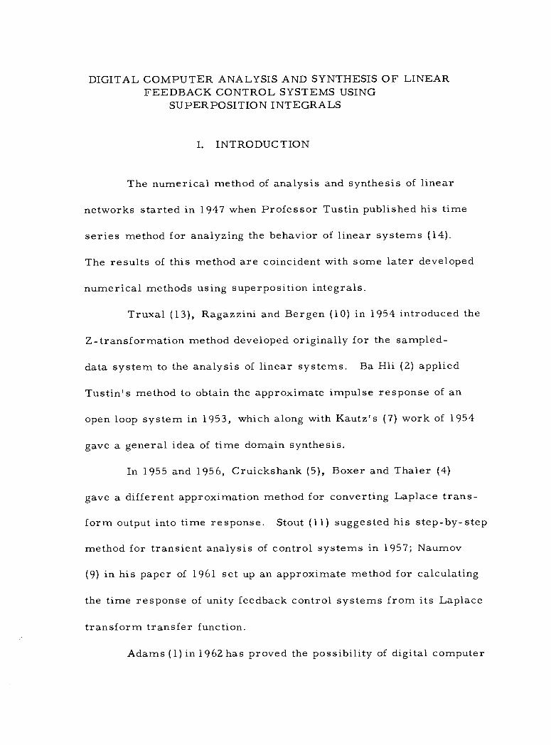
I. INTRODUCTION
The numerical method of analysis and synthesis of linear
networks started in 1947 when Professor Tustin published his time
series method for analyzing the behavior of linear systems (14).
The results of this method are coincident with some later developed
numerical methods using superposition integrals.
Truxal (13), Ragazzini and Bergen (10) in 1954 introduced the
Z- transformation method developed originally for the sampled -
data system to the analysis of linear systems. Ba Hli (2) applied
Tustin's method to obtain the approximate impulse response of an
open loop system in 1953, which along with Kautz's (7) work of 1954
gave a general idea of time domain synthesis.
In 1955 and 1956, Cruickshank (5), Boxer and Thaler (4)
gave a different approximation method for converting Laplace trans-
form output into time response. Stout (11) suggested his step -by -step
method for transient analysis of control systems in 1957; Naumov
(9) in his paper of 1961 set up an approximate method for calculating
the time response of unity feedback control systems from its Laplace
transform transfer function.
Adams (1) in 1962 has proved the possibility of digital computer
2
analysis for unity feedback system from its given transfer func-
tion.
Sometimes, the transfer function of an existing system is
not known. If the system is to be linear or nearly linear, it is
possible to find its impulse response from the input signal and
the output response.
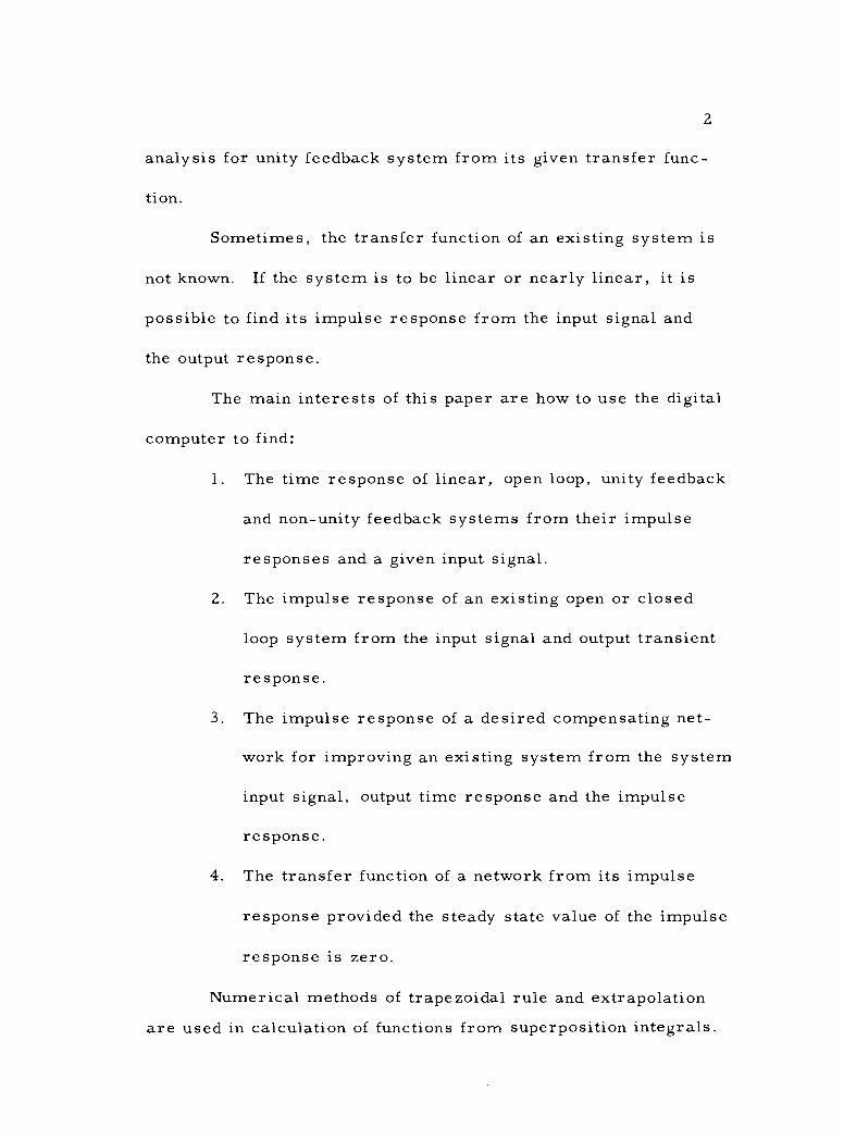
The main interests of this paper are how to use the digital
computer to find:
1. The time response of linear, open loop, unity feedback
and non -unity feedback systems from their impulse
responses and a given input signal.
2. The impulse response of an existing open or closed
loop system from the input signal and output transient
response.
3. The impulse response of a desired compensating net-
work for improving an existing system from the system
input signal, output time response and the impulse
response.
4. The transfer function of a network from its impulse
response provided the steady state value of the impulse
response is zero.
Numerical methods of trapezoidal rule and extrapolation
are used in calculation of functions from superposition integrals.
3
II. ANALYSIS
A. Open Loop System:
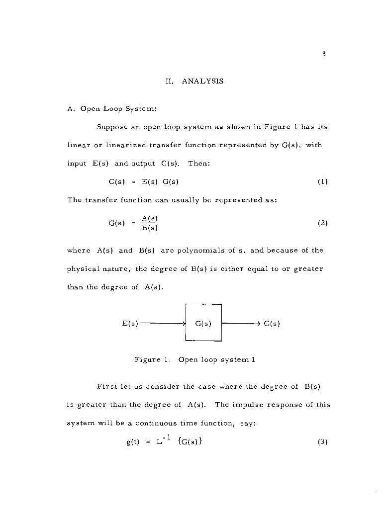
Suppose an open loop system as shown in Figure 1 has its
linear or linearized transfer function represented by G(s), with
input E(s) and output C(s). Then:
C(s) = E(s) G(s) (1)
The transfer function can usually be represented as:
G(s) = A(s) B(s)
(2)
where A(s) and B(s) are polynomials of s, and because of the
physical nature, the degree of B(s) is either equal to or greater
than the degree of A(s).
E(s) G(s)
Figure 1. Open loop system I
> C(s)
First let us consider the case where the degree of B(s)
is greater than the degree of A(s). The impulse response of this
system will be a continuous time function, say:
g(t) = L -1 {G(s)} (3)
4
Since this system is linear, the superposition theorem can be ap-
plied, and the transient time response of the output can be repre-
sented as:
t
c(t) = f e(t-T) g(T) dT (4) o
t or c(t) = r e(T) g(t-T) dT
where
o
e(t) = L-1 { E(s)} ,
the time function of the input voltage.
(5)
(6)
If the numerical values of e(t) and g(t) are known, the
approximate values of the equation (4) or (5) can be calculated
by numerical methods. The simplest numerical integration me-
thod that can be applied to this problem is the trapezoidal rule.
Let the numerical values of e(t) and g(t) at equally spaced
time increments be represented as:
. Time 0 h 2h 3h 4h
e(t) el e2 e3 e4 e5
g(t) g1 g2 g3 g4 g5
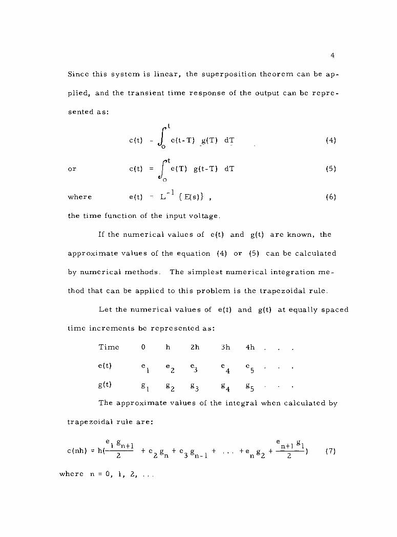
The approximate values of the integral when calculated by
trapezoidal rule are:
e e g c(nh) = h(
1 + e2 gn + e3 gn-1 + + en g2 +
n21 1)
where n = 0, 1, 2, .
(7) g
n +1
2
5
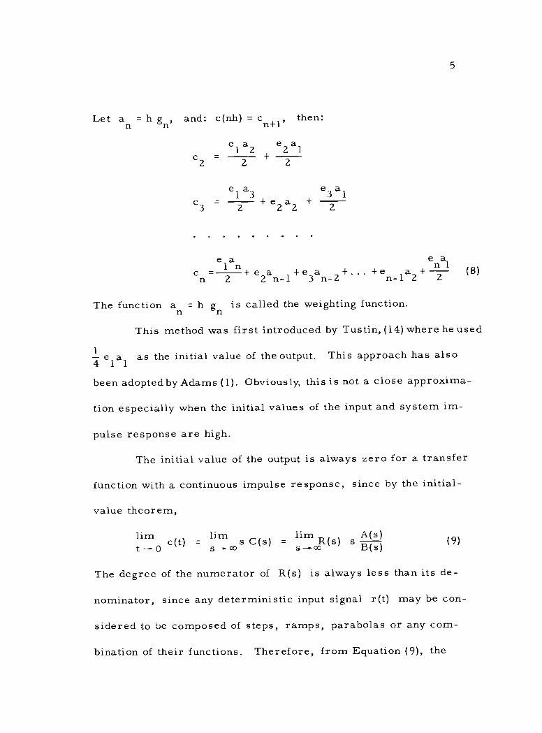
Let an = h gn, and: c(nh) = en +1' then:
el a2 e2a1 c2 =
2 +
2
el a 3
e3 al c3 =
2 + e2 a2 +
2
cn =e 2 elan -1 +e3an -2
+... +en -lag +e 1 (8)
The function an = h gn is called the weighting function.
This method was first introduced by Tustin, (14) where he used
as the initial value of the output. This approach has also 1
elal been adopted by Adams (1). Obviously, this is not a close approxima-
tion especially when the initial values of the input and system im-
pulse response are high.
The initial value of the output is always zero for a transfer
function with a continuous impulse response, since by the initial -
value theorem,
lim lim lim R(s) A(s) (9)
t s- 00 s--.co B(s)
The degree of the numerator of R(s) is always less than its de-
nominator, since any deterministic input signal r(t) may be con-
sidered to be composed of steps, ramps, parabolas or any com-
bination of their functions. Therefore, from Equation (9), the
c(t) sC s ( ) ( ) s
a n
n n
=
6
initial value of c(t) is always zero.
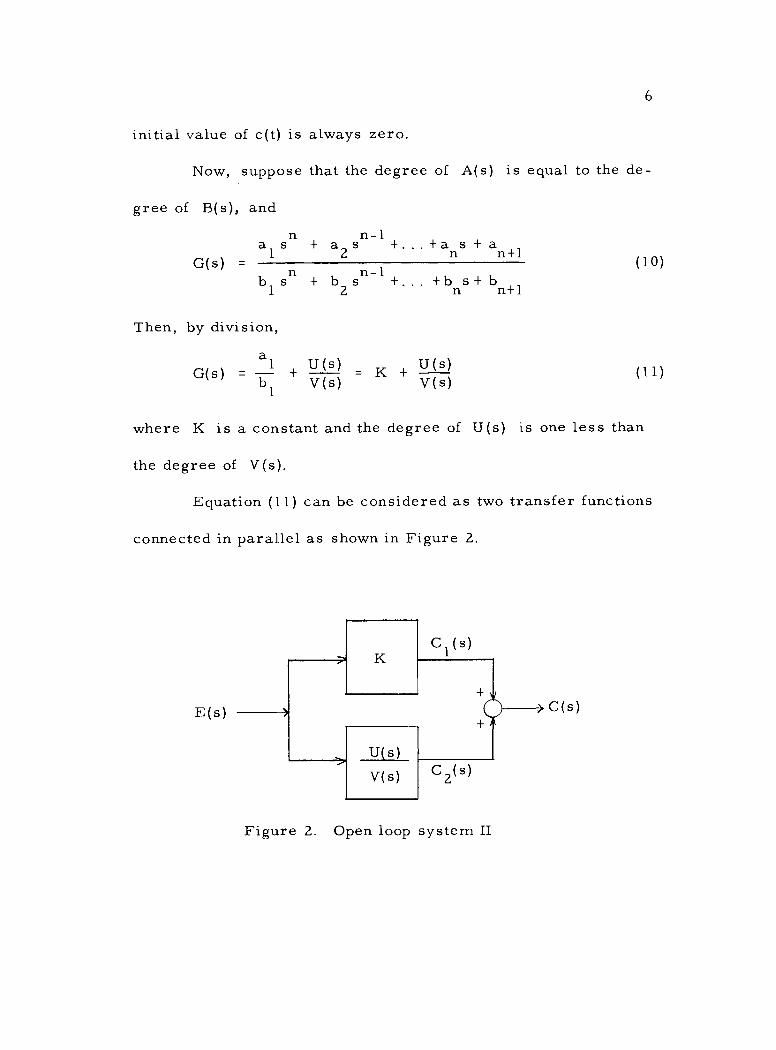
Now, suppose that the degree of A(s) is equal to the de-
gree of B(s), and
G(s) =
n n-1 al s + a2 s +. . . +ans + an+1
bl sn + b2 sn-1 +. . . +bns + bn+1
Then, by division,
G(s) = + U(s) = K + U(s) b1 V(s) V(s)
(10)
where K is a constant and the degree of U(s) is one less than
the degree of V(s).
Equation (11) can be considered as two transfer functions
connected in parallel as shown in Figure 2.
E(s)
K C1(s)
ì U(s)
V(s) C2(s)
Figure 2. Open loop system II
C(s)
(11) 1.
E(s) y
where:
and
From Equation (1 1) and Figure 2,
C(s) = KE(s) + E(s) U(s) V(s)
7
(12)
C1(s) = K E(s) (13)
c (t) 1
= K e(t) (14)
which can be found by:
cln = K en (15)
C = 2(s) E(s) U(s) (16) V(s)
Values for c2(t) can be found by the previous method of continu-
ous impulse response, and:
Since c21 = 0,
cn = cln + c 2 (17)
cl = c11 = Kel
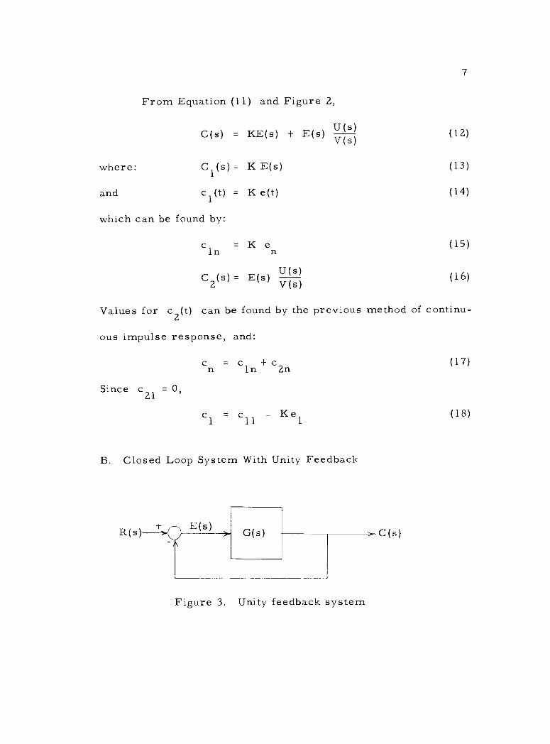
B. Closed Loop System With Unity Feedback
R(s) G(s)
Figure 3. Unity feedback system
C(s)
(18)
n
or:
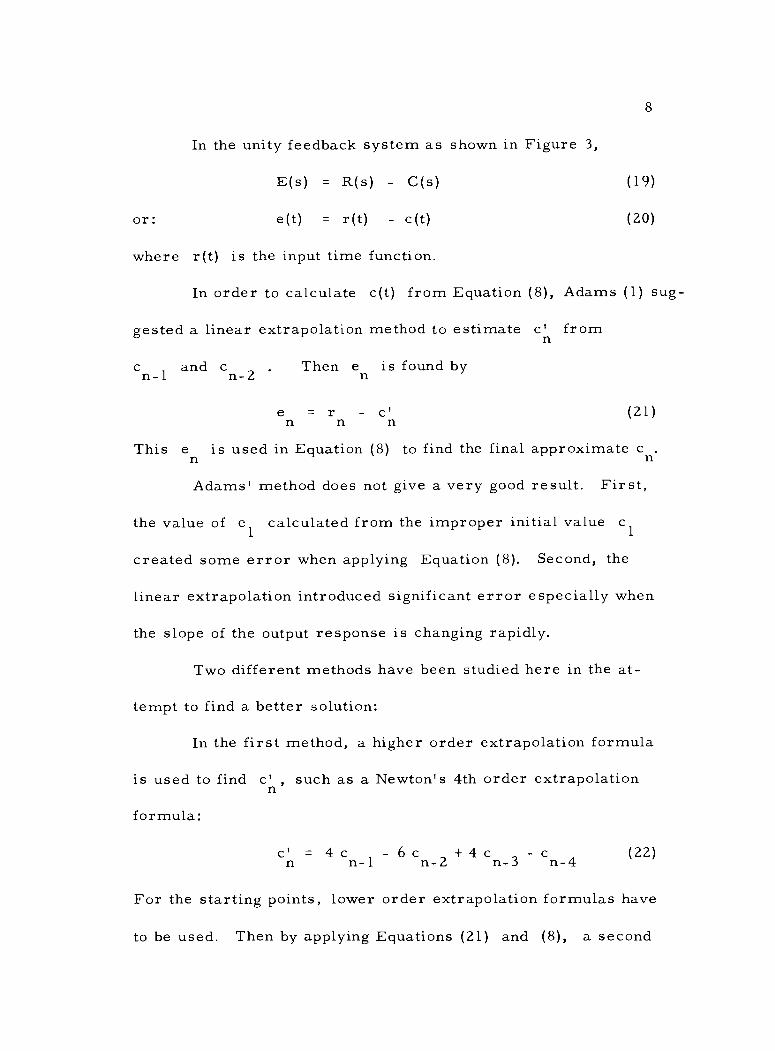
In the unity feedback system as shown in Figure 3,
E(s) = R(s) - C(s)
e(t) = r(t) - c(t)
8
(19)
(20)
where r(t) is the input time function.
In order to calculate c(t) from Equation (8), Adams (1) sug-
gested a linear extrapolation method to estimate c' from
en and en . Then en is found by
e = r - c' n n n
(21)
This en is used in Equation (8) to find the final approximate cn.
Adams' method does not give a very good result. First,
the value of el calculated from the improper initial value cI
created some error when applying Equation (8). Second, the
linear extrapolation introduced significant error especially when
the slope of the output response is changing rapidly.
Two different methods have been studied here in the at-
tempt to find a better solution:
In the first method, a higher order extrapolation formula
is used to find c' , such as a Newton's 4th order extrapolation n
formula:
cñ = 4 cn-1 - 6 cn-2 + 4 en-3 - cn-4 (22)
For the starting points, lower order extrapolation formulas have
to be used. Then by applying Equations (21) and (8), a second
n 2
n
-4

9
approximation c" can be calculated, and this c" may be used
again by applying Equations (21) and (8) to find a more precise
value of c. This c n
may be used as the final approximated
value of the output and the en required in successive calculations n
is obtained by:
e = r - c n n n
(23)
The remaining problem in this method is how to determine
the initial value of the output. The overall transfer function of
the unity feedback system:
G(s) A(s) 1 + G(s) A(s) + B(s) (24)
The degree of the numerator and denominator are the same as the
degree of the numerator and denominator of the transfer function
itself. If the transfer function has a continuous impulse response,
the initial value of the output cl is always zero.
The results of the above method are satisfactory as shown
in Table 2. This method is discarded later however, since it re-
quired laborious calculations.
The second method is derived from Equations (8) and (23).
Since: e an -c ) a
I n n n l cn - + e 2
an-1 + . . + en-la2 + 2
or:
(25) .
n 2
(r
10 elan r a 1
+ e a + . .. + e a + n 1) (26) n al 2 2 n-1 n-1 2 2
2
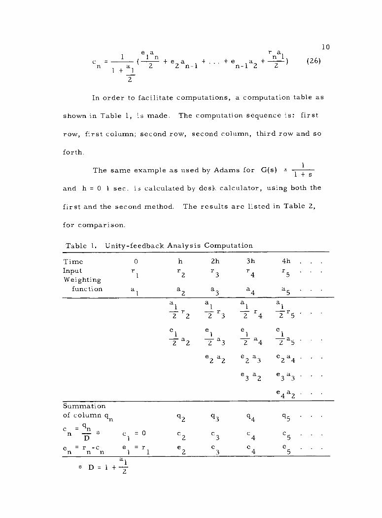
In order to facilitate computations, a computation table as
shown in Table 1, is made. The computation sequence is: first
row, first column; second row, second column, third row and so
forth.
The same example as used by Adams for G(s) = 1 + s
and h = 0 1 sec. is calculated by desk calculator, using both the
first and the second method. The results are listed in Table 2,
for comparison.
Table 1. Unity- feedback Analysis Computation
1
Time 0 h 2h 3h 4h .
Input r r2 r3 r4 r5 .
Weighting function al a2 a3 a4 a5 .
a1 a1 al a1
2 r2 2 r3 2 r4 -z r5 '
el el el el
2 a2
2 a3 a4 -27 as
'
e2 a2 e2 a3
e3 a2
e2 a4
e3 a3
e4 a2
Summation of column qn q2 q3 q4 q5
q cn D
-, cl = 0 c2 c3 c4 c5
en - rn-Cn el - rl e2 e3 e4 e5 al
,- D = 1 + 7
n+
2
.
=
1
.
=
]
.
11
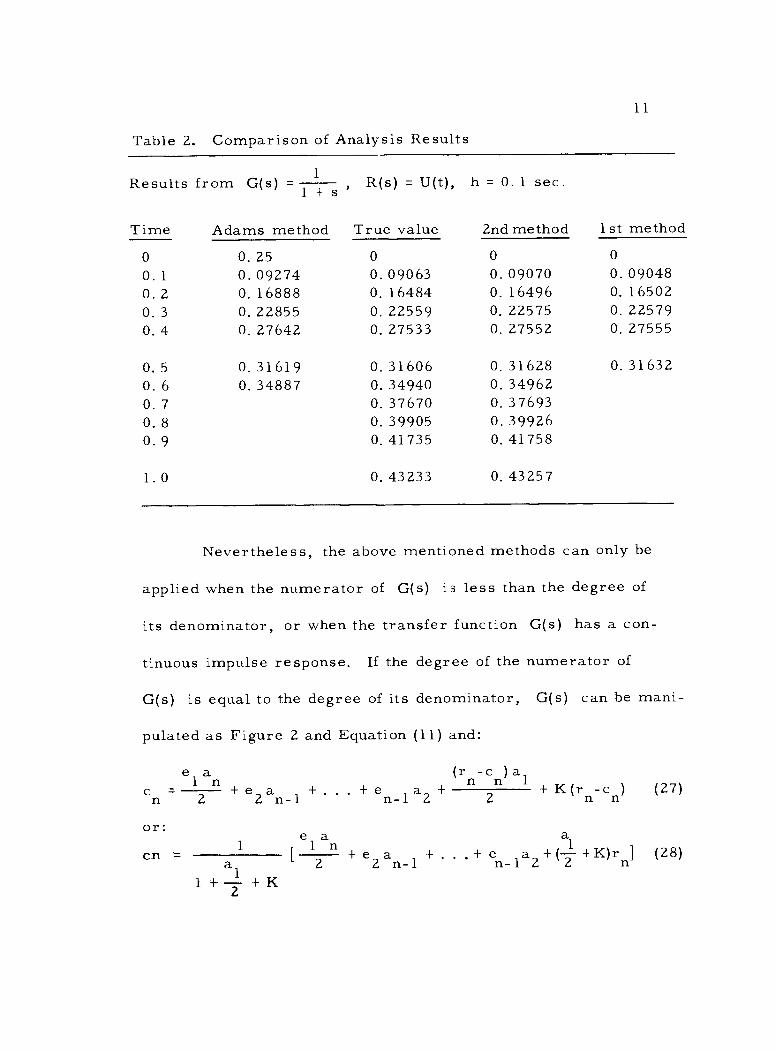
Table 2. Comparison of Analysis Results
Results
Time
from G(s) ,
R(s) = U(t),
True value
h = 0. 1 sec.
2nd method 1st method
= 1 + s
Adams method
0 0. 25 0 0 0
0. 1 0.09274 0.09063 0.09070 0.09048 0.2 0. 16888 0. 16484 0. 16496 0. 16502 0.3 0.22855 0.22559 0. 22575 0.22579 0.4 0. 27642 0. 27533 0. 27552 0. 27555
0.5 0.31619 0.31606 0. 31628 0.31632 0. 6 0. 34887 0. 34940 0. 34962 0.7 0. 37670 0. 37693 0, 8 0. 39905 0. 39926 0.9 0.41735 0.41758
1.0 0.43233 0.43257
Nevertheless, the above mentioned methods can only be
applied when the numerator of G(s) is less than the degree of
its denominator, or when the transfer function G(s) has a con-
tinuous impulse response. If the degree of the numerator of
G(s) is equal to the degree of its denominator, G(s) can be mani-
pulated as Figure 2 and Equation (1 1) and:
el an c + e a + . . . + e a + (rn-cn) al
K n 2 2 n-1 n-1 2 2 n n
or: el a a cn = al [
n -I- elan + . . . + ñ- la2 + (-2 +K)rn] (28)
1 +Z+K
1
The value of
or:
cl = K el =K (r 1
- cl)
K r 1
cl 1+K
12
(29)
(30)
Therefore, the initial value of the output is always less than the initial
value of the input signal when K> O. When K = 0, Equation (28) equals
Equation (26) and cl = O.
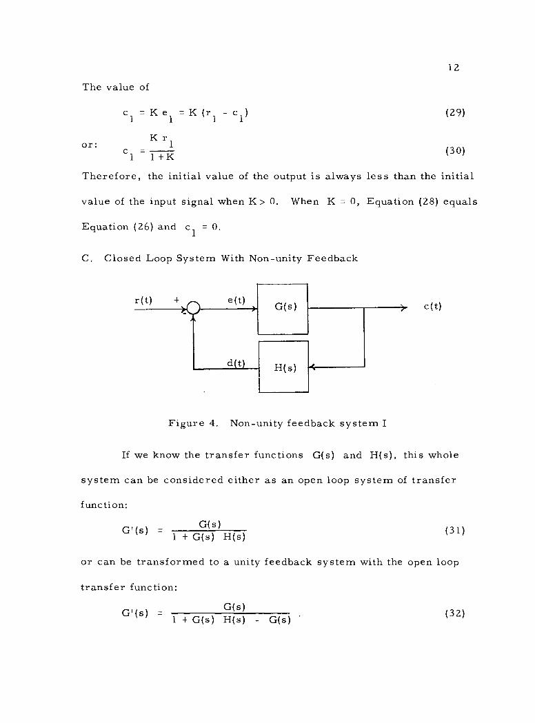
C. Closed Loop System With Non -unity Feedback
Figure 4. Non -unity feedback system I
c(t)
If we know the transfer functions G(s) and H(s), this whole
system can be considered either as an open loop system of transfer
function:
G'(s) - G(s) 1 + G(s) H(s) (31)
or can be transformed to a unity feedback system with the open loop
transfer function:
GIs) = G(s)
1 + G(s) H(s) - G(s) (32)
r(t) + e(t) )
d(t)
G(s)
H(s)
13
Then, if the impulse response of either of the above transfer
functions can be calculated, c(t) can be calculated by one of
the previous methods. Suppose the impulse responses g(t) and
h(t) are given as:
Time 0 h 2h 3h 4h
g(t) g1 g2 g3 g4 g5
h(t) hl h2 h3 h4 h5
at equally spaced time increments, and it is known that they are
both continuous. Then: c = dl = 0, el = r and:
el an en al co - + e2
an-1 + . . . + en-1 a2 + 2
c bn cobl do = + c2bn-1 + . . . + co-1 b2 + 2
(33)
(34)
en = r n
- d n
(35)
where:
an and b =hh n n n n
Solving Equations (33), (34) and (35),
cn = 1 [ 1 a r + 1 elan + e a + . .. + e a n 1+ 1 a b
2 1 n 2 elan 2 n-1 n-1 2
4 1 1
4a1 (b +c b + +c b )] (36) 2-c 1 n 2 n-1 , ,, n-1 2
If the degree of the numerators of both G(s) and H(s)
are equal to the degree of their denominators, Figure 4 can be
n -
n
.
. .
2 n2 1
= h gn
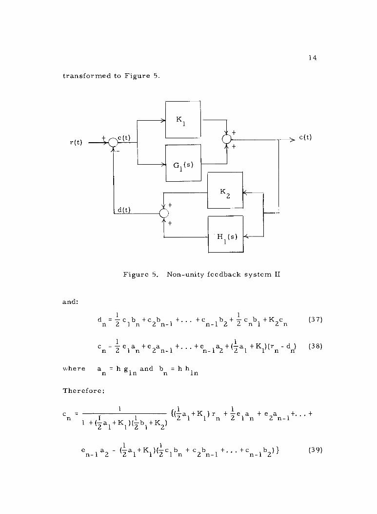
transformed to Figure 5.
r(t)
and:
e(t)
d(t)
K 1
G1(s)
K2
H1(s)
Figure 5. Non -unity feedback system II
14
c(t)
dn= 2 clbn+c2bn-1 +. . . +cn-1b2+ 2 cnbl +K2cn (37)
c n 2
=-e 1
elan n
+e 2 a n-1 +. . . +e n-1 a
2 +(1 a
2 1 +K
1 )(r
n - d n ) (38)
where an = h gin and bn = h hln
Therefore:
1 c = 1 l + e +K )r a +e a +...+
n 1+ l +K a )(-b l +K 2 1 1 n 2 1 n 2 n-1 (2 1 1)(2 1 2)
e a - (1 a +K )(1 c b + c b +. . . +c b ) } n-1 2 2 1 1 2 1 n 2 n-1 n-1 2
(39)
Y+
l n
The value of
cl r K
1 1
1 +K1K2
15
(40)
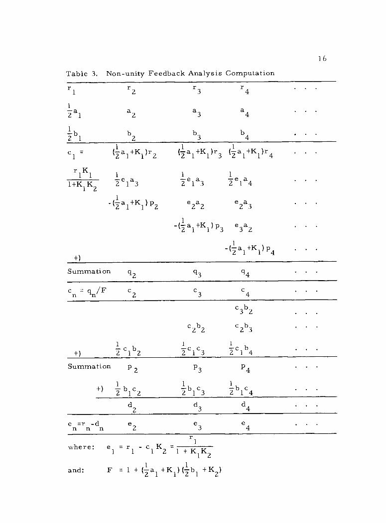
When K1 = K2 = 0, Equation (39) is equal to Equation (36). Table
3 shows the computation procedure.
-
16
Table 3. Non -unity Feedback Analysis Computation
r r2 r3 r4
1
2a1 al a2 a3 a4
2 ó1 ó2 b3 2 1 2 ó4
c = (1 a +K )r (1 a +K )r (1 a +K )r 1 2 1 1 2 1 1 3 2 1 1 4
r1K1 1 -1 e
1
1+K1K2 2e1a3 21a3 2e1a4
21+K1)p2
+)
e2a2
1
-(2 a1+K1) p
e2a3
e3a2
- (la +K1) p4
Summation q2 q3 q4
cn = qn/F c 2
c3 c4
+)
c2b2
c3b2
c2 b 3
2 c1b2 2c1c3 2c1ó4
Summation P 2 p3 p4
1 -1 b +)
2 ó1 c2 2 c3 ól
2 c4 ól
d2 d3 d4
e =r -d e2 e3 e4 4
where: el = r 1 - cl K2 1+ K K
1 2
r 1
and: F = 1 + (-2-al +K1) (2b1 +K2)
2
- 2
1
n n n 2
1
17
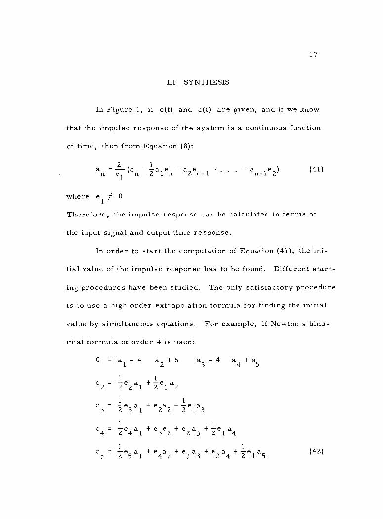
III. SYNTHESIS
In Figure 1, if e(t) and c(t) are given, and if we know
that the impulse response of the system is a continuous function
of time, then from Equation (8):
2 1
an = e
(cn - 2 al en - a2en-1 . - a e n-12) (41)
where el / 0
Therefore, the impulse response can be calculated in terms of
the input signal and output time response.
In order to start the computation of Equation (41), the ini-
tial value of the impulse response has to be found. Different start-
ing procedures have been studied. The only satisfactory procedure
is to use a high order extrapolation formula for finding the initial
value by simultaneous equations. For example, if Newton's bino-
mial formula of order 4 is used:
0 = a 1
-4 a2+6 a3 - 4 a4+a5
1 1 c2 = e2 al + 2e1 a2
1 1 c3 = 2e3 al + e2a2 + 2 ela3
1 1 c4 = -2e 4
al + e3e2 + e2a3 + 2el a4
1 1 c = 2 2 a +ea+ea +ea+ea (42)
- . .
5 1 4 2 3 3 4
18
Solving the above equations - by using a digital computer, the
first five values of the impulse response can be found, and the
successive values can be computed by applying Equation (41).
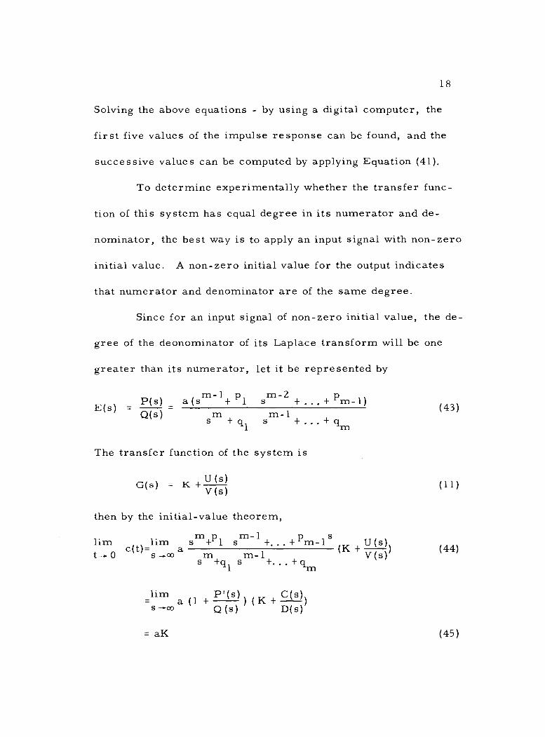
To determine experimentally whether the transfer func-
tion of this system has equal degree in its numerator and de-
nominator, the best way is to apply an input signal with non -zero
initial value. A non -zero initial value for the output indicates
that numerator and denominator are of the same degree.
Since for an input signal of non -zero initial value, the de-
gree of the deonominator of its Laplace transform will be one
greater than its numerator, let it be represented by
E(s) = P(s) - Q(s)
(sm-1+ p1
sm-2 + . . . + pm-1)
sm + gl sm-1 + . . . + gm
The transfer function of the system is
G(s) = K + U(s) V(s)
(43)
then by the initial -value theorem,
lim c(t)_lim a
sm +pl sm -1 +... +pm -ls +U(s)) t- 0 s -co sm+ sm- 1 +... +
V(s) +q qm
_lim (1 + PI(s) ) ( K + C(s)) s Q(s) D(s)
= aK (45)
a
... (K (44)
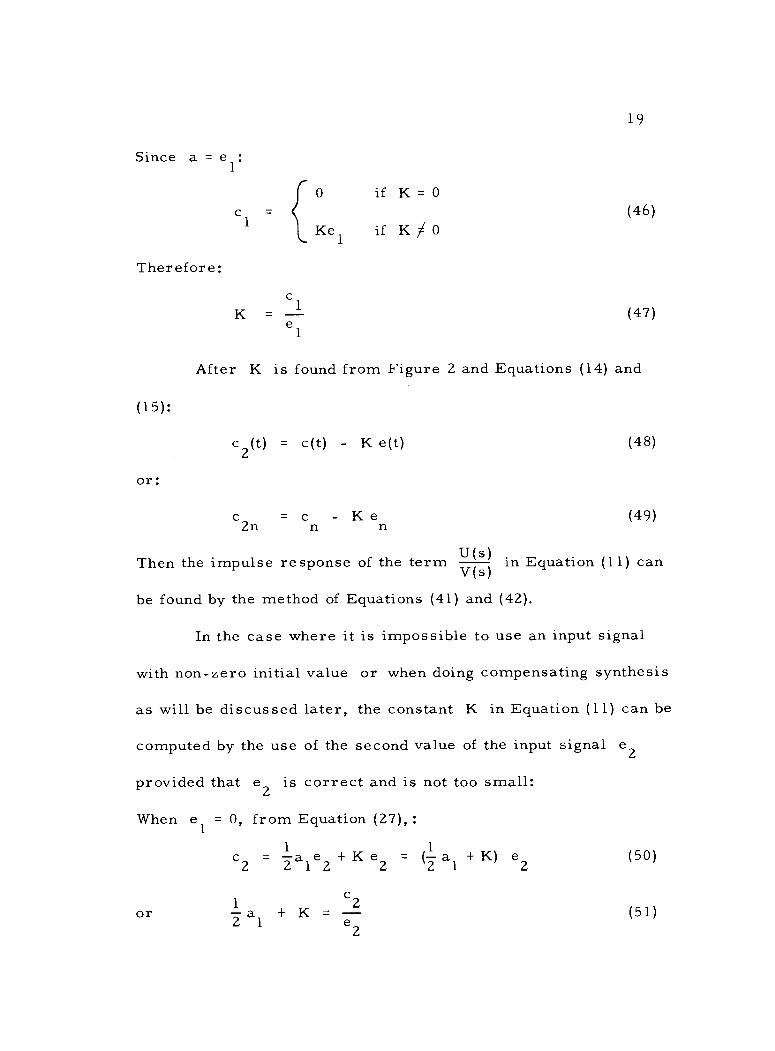
Since a = e : 1 1
Therefore:
(15):
or:
cl
c
K = 1 el
0 if K =
Kel if K#0
19
(46)
(47)
After K is found from Figure 2 and Equations (14) and
c2(t) = c(t) - K e(t) (48)
c2n = cn - Ken (49)
Then the impulse response of the term U(s) V(s)
in Equation (1 1) can
be found by the method of Equations (41) and (42).
In the case where it is impossible to use an input signal
with non -zero initial value or when doing compensating synthesis
as will be discussed later, the constant K in Equation (11) can be
computed by the use of the second value of the input signal e2
provided that e2 is correct and is not too small:
When e 1
= 0, from Equation (27), :
c2 = 2a 1e2 + K e2 = (-1 al + K) e2
c
or 2al + K = 2 e 2
(50)
(51)
=
0
20
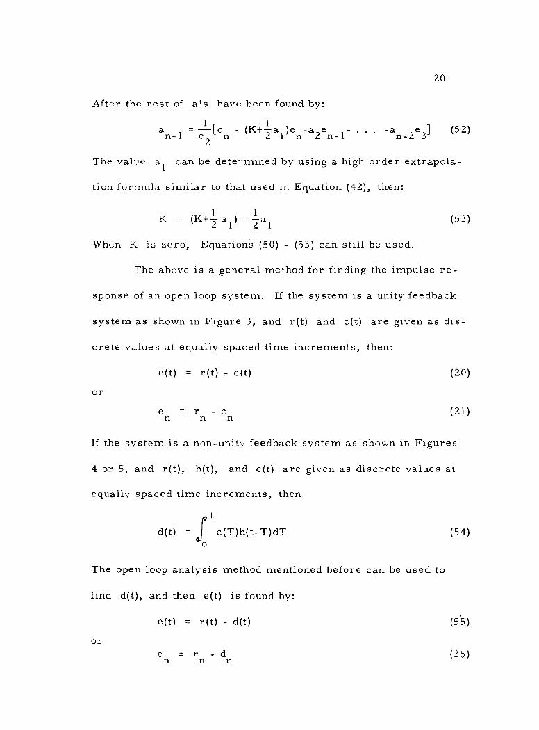
After the rest of a's have been found by:
-1 e2 [cn (K+ 2 a1)en- aten -1- . . . - an -2e3] (52)
The value al can be determined by using a high order extrapola-
tion formula similar to that used in Equation (42), then:
K = (K+2 al) - 2al (53)
When K is zero, Equations (50) - (53) can still be used.
The above is a general method for finding the impulse re-
sponse of an open loop system. If the system is a unity feedback
system as shown in Figure 3, and r(t) and c(t) are given as dis-
crete values at equally spaced time increments, then:
e(t) = r(t) - c(t) (20)
or
en r - c n n n
(21)
If the system is a non -unity feedback system as shown in Figures
4 or 5, and r(t), h(t), and c(t) are given as discrete values at
equally spaced time increments, then
d(t) _
t
c(T)h(t-T)dT
The open loop analysis method mentioned before can be used to
find d(t), and then e(t) is found by:
e(t) = r(t) - d(t)
or en r - d
n n n
(54)
(55)
(35)
-
o
=
21
From the computed e(t) and the given c(t), the required g(t)
can be found.
If the impulse response found from the above is mainly
for analysis use, there is no need to convert it to the frequency
domain. The method for finding the equivalent transfer function
of certain system with given impulse response will be discussed
in the next section.

22
IV. COMPENSATION OF CONTROL SYSTEM
A. Compensation
Suppose a control system as shown in Figure 3 or 4 is
given. If the time response of the system when computed by the
analysis method mentioned before does not give a satisfactory re-
sult, usually, a series or feedback compensating circuit can be
used to improve the output response as shown in Figure 6 and
Figure 7
r(t) ± e(t)
d(t)
F(s)
H(s)
G(s)
Figure 6. Series compensating system
r(t) ± e(t) A
d(t) F(s)
G(s)
k(t) H(s)
Figure 7. Feedback compensating system
c(t)
i c(t)
L
23
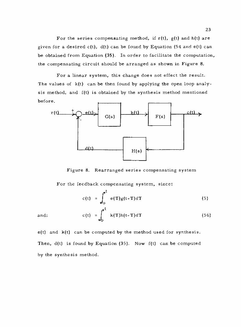
For the series compensating method, if r(t), g(t) and h(t) are given for a desired c(t), d(t) can be found by Equation (54 and e(t) can
be obtained from Equation (35). In order to facilitate the computation,
the compensating circuit should be arranged as shown in Figure 8.
For a linear system, this change does not effect the result.
The values of k(t) can be then found by applying the open loop analy-
sis method, and f(t) is obtained by the synthesis method mentioned
before.
r(t) e(t) k(t) G(s)
H(s)
F(s) c(t) >
Figure 8. Rearranged series compensating system
For the feedback compensating system, since: t
c(t) = fo e(T)g(t -T)dT
and: c(t) = k(T)h(t- T)dT
e(t) and k(t) can be computed by the method used for synthesis.
Then, d(t) is found by Equation (35). Now f(t) can be computed
by the synthesis method.
(5)
(56)
1n
0
24
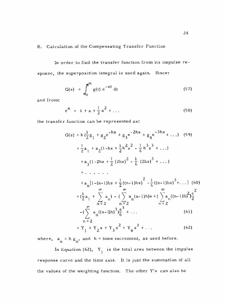
B. Calculation of the Compensating Transfer Function
In order to find the transfer function from its impulse re-
sponse, the superposition integral is used again. Since:
and from: :
co
G(s) = J
g(t) e-st dt
ex = 1 +x+2x2+...
the transfer function can be represented as:
G(s) = h (- g 2 1
+ g2e-hs g3e-2hs g4e-3hs
= 2a1 + a2(1-hs + 2 s2
- 6
3 3 hs + .
+a3(1-2hs + Z
(2hs)2 - 6
(2hs)3 + . ,. )
(57)
(58)
.) (59)
+an[1-(n-1)hs + 2((n-l)hs)2 - 6 ((n-1)hs)3+. . . ] (60)
oo co
1 _ (-2-al +
L an) - ( an(n- 1)h)s + (
n=2 n=2 °n 3
an((n-1)h)3)ó + . . .
n=2 = Y1 + Y2 s + Y3 s2 + Y4 s3 + . . .
00 2
((n- 1)h)2)2
(61)
(62)
where, an = h g , n
and h = time increment, as used before.
In Equation (62), Y1 is the total area between the impulse
response curve and the time axis. It is just the summation of all
the values of the weighting function. The other Y's can also be
s
+
n=2
25
calculated from the weighting function.
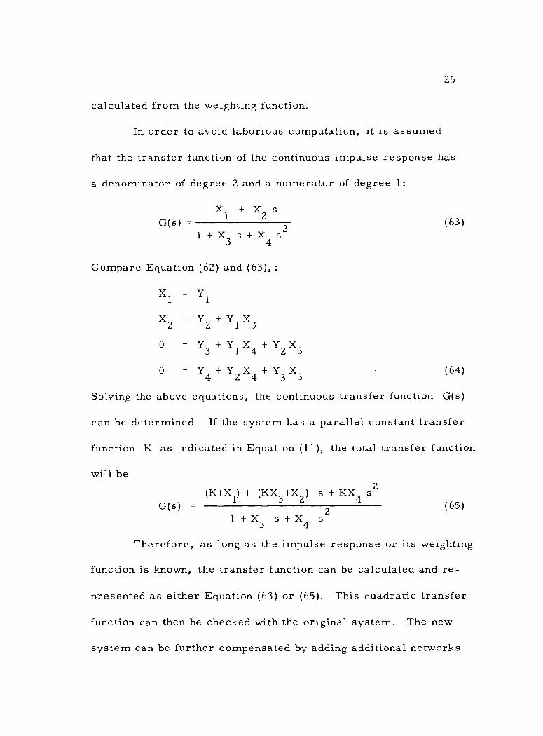
In order to avoid laborious computation, it is assumed
that the transfer function of the continuous impulse response has
a denominator of degree 2 and a numerator of degree 1:
X + X 2
s G(s) = 1 (63)
1 + X3 s + X4 s
Compare Equation (62) and (63), :
X1 = Y1
X2 = Y2 + Y1 X3
0 = Y3 + Y1 X4 + Y2 X3
0 = Y4 + Y2 X4 + Y3 X3 (64)
Solving the above equations, the continuous transfer function G(s)
can be determined. If the system has a parallel constant transfer
function K as indicated in Equation (11), the total transfer function
will be
G(s) - (K+X1) + (KX3+X2) s + KX4 s2
1 +X3 s +X4 s 2
(65)
Therefore, as long as the impulse response or its weighting
function is known, the transfer function can be calculated and re-
presented as either Equation (63) or (65). This quadratic transfer
function can then be checked with the original system. The new
system can be further compensated by adding additional networks
26
of the form of Equations (63) or (65). These networks are found by
applying the above method. With this compensating procedure, or-
dinary systems can always be compensated.

V. EXAMPLES AND THEIR ACCURACY
A. Analysis
27
Several examples similar to those used in Adams' paper
have been computed by using the IBM 1620. Different time incre-
ments were used in order to find the best choice, i. e. satisfactory
results and not too laborious computation. The conclusions are:
1. Find the time from the given impulse response curve
where the value has decreased to about 1100 of the maximum
value; say T.
2. Choose the time increment h equal to T divided by
a convenient number around 60 to 80, and choose T as the com-
puting range. Since beyond T, the response will be approaching
steady state.
3. Compute the output response, from which find a new
T. The value of T should be just large enough to include the en-
tire transient period. This T will be divided by a convenient
number around 70 to find a new h; then compute again. The final
results will give a response accurate to the third place.
The IBM 1620 takes about one minute acutal computing
time (input time are not included) to compute the output of an open
loop or an unity feedback system. It will take four minutes to
28
compute a non -unity feedback system output. This is about 1/3 to
1/4 the time required by Adams' method to attain comparable ac-
curacy using the same digital computer.
B. Synthesis
In order to find the impulse response only, a similar pro-
cedure as stated above can be used. If the response value at T
has decreased to about 1100 of its maximum value and the divisor
is around 70, the error will be less than 1/500 of the response
maximum value.
In order to find the equivalent transfer function of the impulse
response, the computing range should be longer. The value of the
impulse response at T should be around 110000 to 1/100000 of its maxi-
mum in order to find accurate coefficients. The divisor is chosen as 100.
It takes about one minute to compute the impulse response on
the IBM 1620. The equivalent transfer function can be calculated in
about nine minutes.
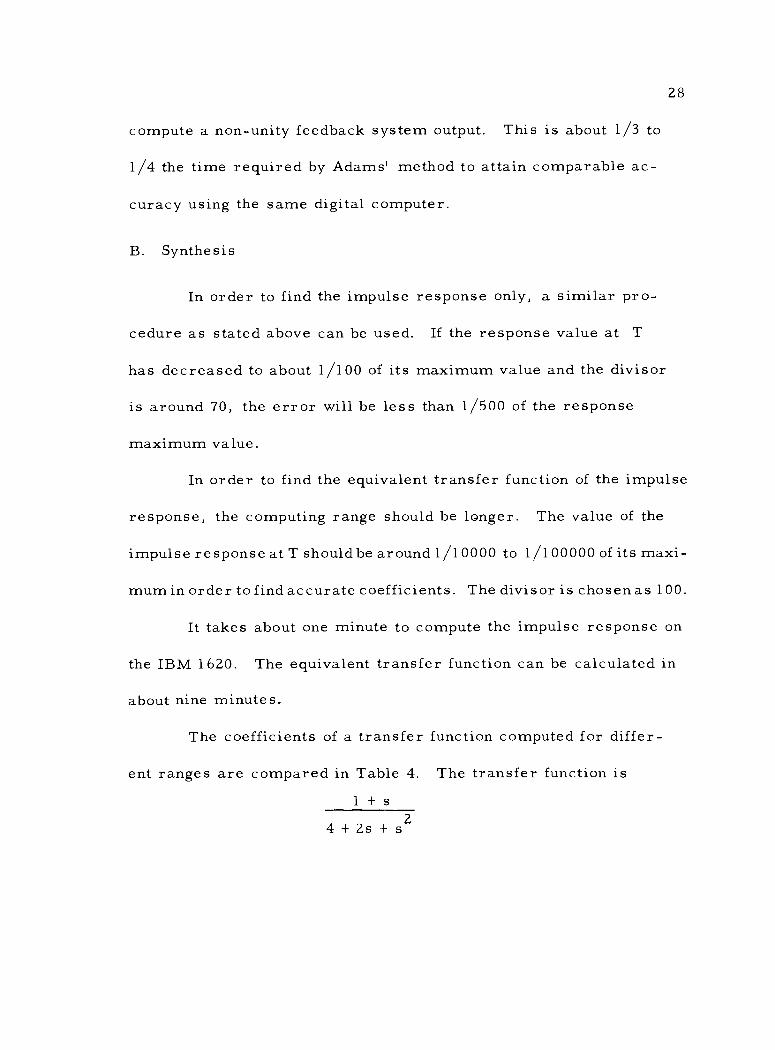
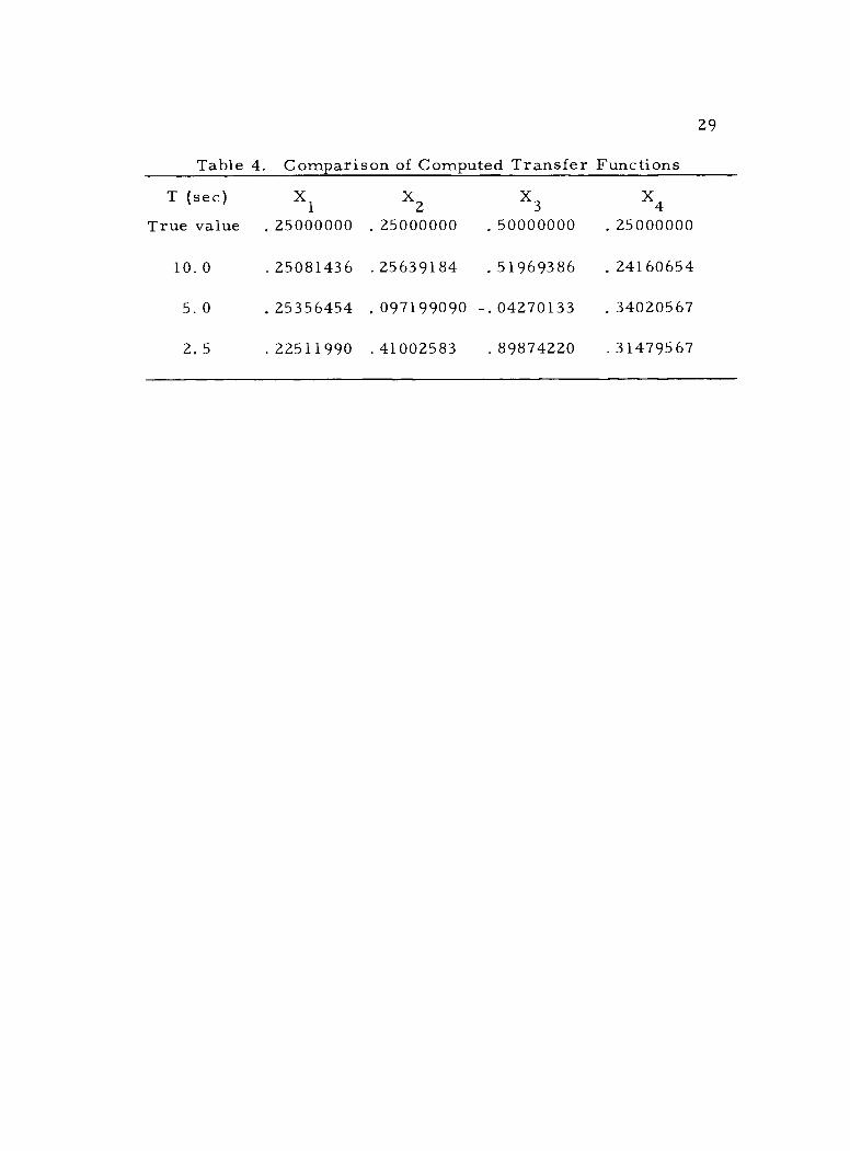
The coefficients of a transfer function computed for differ-
ent ranges are compared in Table 4. The transfer function is
1 + s
4 +2s +s2
29
Table 4. Comparison of Computed Transfer Functions
T (sec) X1 X2 X3 X4
True value .25000000 .25000000 .50000000 .25000000
10.0 . 25081436 . 25 63 9184 .51969386 . 24160654
5. 0 . 2535 6454 . 097199090 -.04270133 . 340205 67
2. 5 . 22511990 .41002583 . 89874220 .314795 67
30
VI. CONCLUSION
The methods represented in this paper furnish a practical
way to analyze almost any kind of linear control system provided
that it is stable. They also give an accurate method to compen-
sating an existing system. The synthesis method mentioned in
this paper provides a simple procedure for directly converting a
computed impulse response to its transfer function. The impulse
response can be obtained for any kind of an input signal and a
reasonable output response. A complete synthesis program writ-
ten in Fortran is contained in the appendix for reference.
Common types of non - linear and time varying systems can
also be solved by numerical methods. Analysis methods appear
in some of the papers contained in the attached bibliography.
It is hoped that high speed digital computers can be used
along with analog -digital converters to solve routine problems
for control engineers. The methods presented in this paper give a
fundamental technique for this purpose.
31
BIBLIOGRAPHY
1. Adams, R. K. Digital computer analysis of closed -loop systems using the number series approach. American Institute of Electrical Engineers Transactions, Part II (Applications and Industry) 80 :370 -378. Jan. 1961.
2. Ba Hli, Freddy. A general method for time domain network synthesis. Institute of the Radio Engineers Transactions on Circuit Theory CT -2:21 -28. 1954.
3. Boxer, Rubin. A note on numerical transform calculus. Proceedings of the Institute of Radio Engineers 45:1401- 1406. 1957.
4. Boxer, Rubin and Samuel Thaler. A simplified method of solving linear and nonlinear systems. Proceedings of the Institute of Radio Engineers 44:89 -101. 1956.
5. Cruickshank, A. J. O. A note on time series and the use of jump functions in approximate analysis. Proceedings of the Institution of Electrical Engineers, Part C (Monographs) 102:81-87. 1954.
6. D'Azzo, John J. and Constantine H Houpis. Feedback control system analysis and synthesis. McGraw -Hill, New York, 1960. 580 p.
7. Kautz, William H. Transient synthesis in the time domain. Institute of the Radio Engineers Transactions on Circuit Theory CT- 2:29 -39. 1954.
8. Milne, William Edmund. Numerical calculus. Princeton, Princeton University, 1949. 393 p.
9. Naumov, B. Approximate method for calculating the time response in linear, time -varying, and nonlinear automatic control systems. Transactions of the American Society of Mechanical Engineers, Journal of Basic Engineering 83:109- 118. March 1961.
32
10. Ragazzini, J. R. and A. R. Bergen. A mathematical techni- que for the analysis of linear systems. Proceedings of the Institute of Radio Engineers 42:1645 -1651. 1954.
11. Stout, T. M. A step -by -step method for transient analysis of feedback systems with one nonlinear element. American Institute of Electrical Engineers Transactions, Part II (Applications and Industry) 75:378 -390. 1956.
12. Thaler, Samuel and Rubin Boxer. An operational calculus for numerical analysis. The Institute of Radio Engineers Convention Record, Part 2 (Circuit Theory) 4:100 -105. 1956.
13. Truxal, John G. Numerical analysis for network design. Institute of the Radio Engineers Transactions on Circuit Theory CT - 2:49 -60. 1954.
14. Tustin, A. A method of analysing the behaviour of linear system in terms of time series. The Journal of the Institution of Electrical Engineers, Part IIA, Proceedings at the Convention on Automatic Regulators and Servo Mechanisms 94:130 -142. 1947.

APPENDICES
33
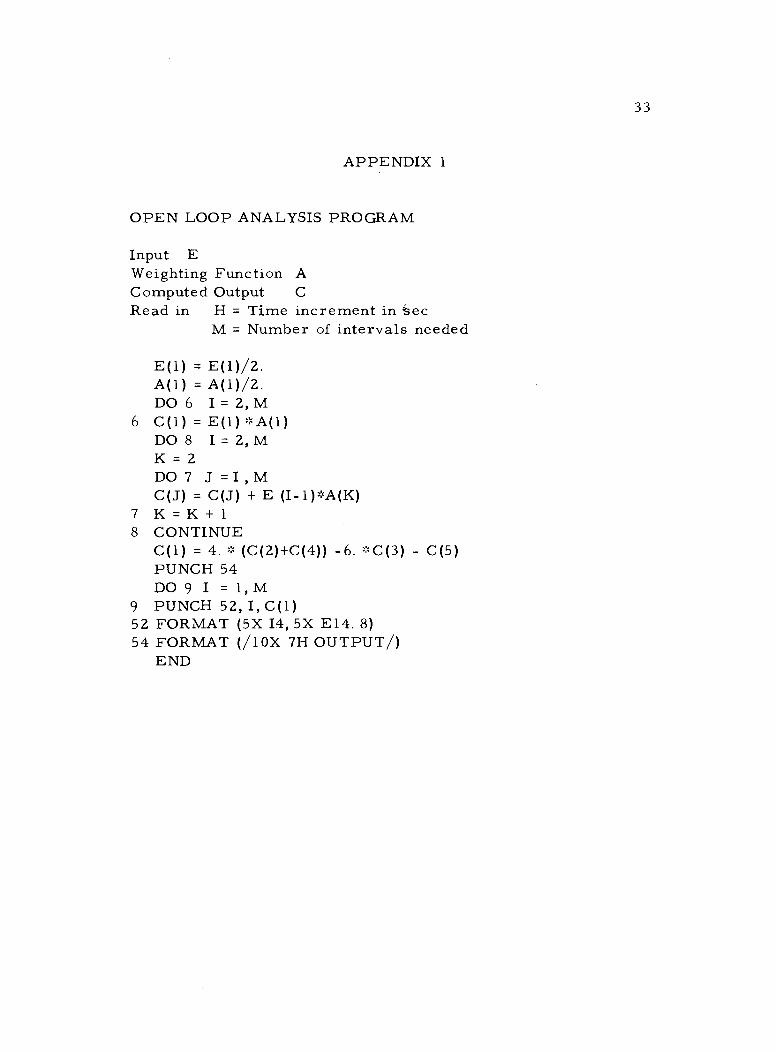
APPENDIX 1
OPEN LOOP ANALYSIS PROGRAM
Input E Weighting Function A Computed Output C Read in H = Time increment in sec
M = Number of intervals needed
E(1) = EGO. A(1) = A(1)/2. DO 6 I= 2,M
6 C(1) = E(1) *A(1) DO8 I=2,M K = 2
DO7 J=I,M C(J) = C(J) + E (I-1)*A(K)
7 K = K + 1
8 CONTINUE C(1) = 4.* (C(2)+C(4)) -6. *C(3) - C(5) PUNCH 54 DO 9 I = 1, M
9 PUNCH 52, I, C(1) 52 FORMAT (5X 14, 5X E14. 8) 54 FORMAT (/10X 7H OUTPUT/)
END
34
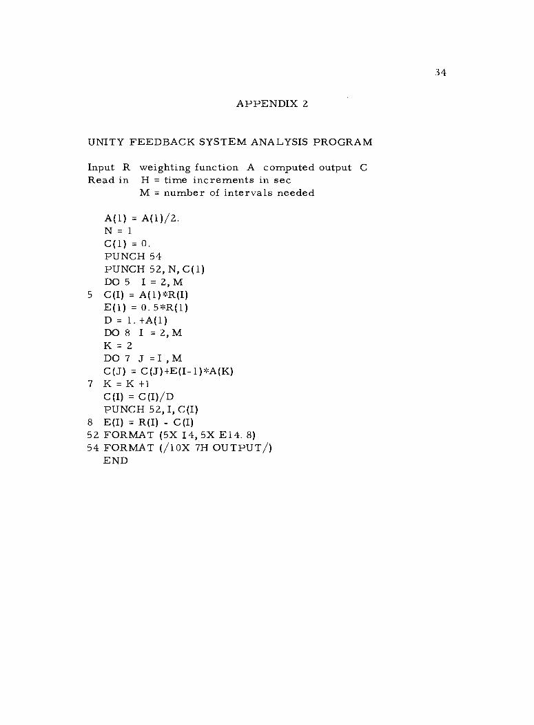
APPENDIX 2
UNITY FEEDBACK SYSTEM ANALYSIS PROGRAM
Input R weighting function A computed output C Read in H = time increments in sec
M = number of intervals needed
A(1) = A(1)/2. N = 1
C(1) = O.
PUNCH 54 PUNCH 52, N, C(1) DO5 I=2,M
5 C(I) = A(1)*R(I) E(1) = 0.5*R(1) D = 1. +A(1) DO 8 I = 2,M K = 2
DO 7 J =I ,M C(J) = C(J)+E(I-1)*A(K)
7 K=K+1 C(I) = C(I)/D PUNCH 52, I, C(I)
8 E(I) = R(I) - C(I) 52 FORMAT (5X I4, 5X E14. 8) 54 FORMAT (/10X 7H OUTPUT/)
END
35
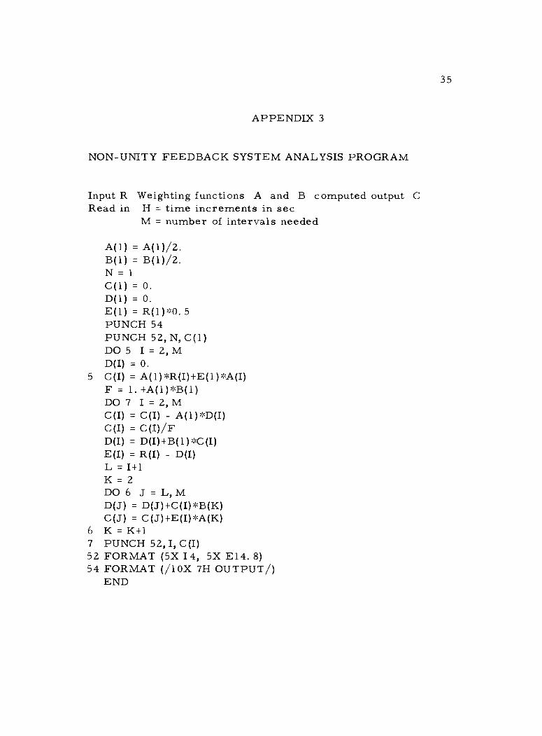
APPENDIX 3
NON -UNITY FEEDBACK SYSTEM ANALYSIS PROGRAM
Input R Weighting functions A and B computed output C Read in H = time increments in sec
M = number of intervals needed
A(1) = A(1)/2. B(1) = B(1)/2. N = 1
C(1) = O.
D(1) = O.
E(1) = R(1)*O. 5
PUNCH 54 PUNCH 52, N, C(1) DO 5 I = 2,M D(I) = O.
5 C(I) = A(1)*R(I)+E(i)*A(I) F = 1. +A(1)*B(1) DO 7 I = 2,M C(I) = C(I) - A(1)*D(I) C(I) = C(I)/F D(I) = D(I)+B(1) *C (I) E(I) = R(I) - D(I) L = 1+1 K = 2
DO6 J=L,M D(J) = D(J)+C(I)*B(K) C(J) = C(J)+E(I) *A(K)
6 K=K+1 7 PUNCH 52, I, C(I) 52 FORMAT (5X I4, 5X E14. 8) 54 FORMAT (/10X 7H OUTPUT/)
END
36
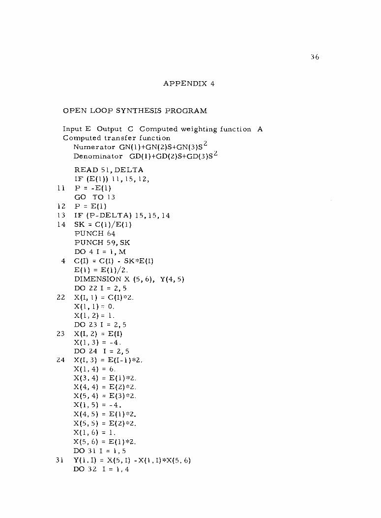
APPENDIX 4
OPEN LOOP SYNTHESIS PROGRAM
Input E Output C Computed weighting function A Computed transfer function
Numerator GN(1) +GN(2)S +GN(3)S2 Denominator GD(1) +GD(2)S +GD(3)S2
READ 51, DELTA IF (E(1)) 11, 15, 12,
11 P = -E(1) GO TO 13
12 P = E(1) 13 IF (P- DELTA) 15, 15, 14 14 SK = C(1) /E(1)
PUNCH 64 PUNCH 59, SK DO 4I = 1, M
4 C(I) = C(I) - SK *E (I) E(1) = E(1)O2. DIMENSION X (5, 6), Y(4, 5) DO 22 I = 2, 5
22 X(I, 1) = C(I) *2. X(1, I) =O. X(1, 2) = 1.
DO 23I =2,5 23 X(I, 2) = E(I)
X(1,3) _ -4. DO 24 I = 2, 5
24 X(I, 3) = E(I -1) *2 X(1, 4) = 6. X(3,4) = E(1)*2. X(4, 4) = E(2) *2. X(5, 4) = E(3) *2. X(1,5) = -4. X(4,5) = E(1) *2. X(5, 5) = E(2) *2. X(1, 6) = 1. X(5, 6) = E(1) *2. DO31I = 1,5
31 Y(1, I) = X(5, I) -X(1,I) *X(5, 6) DO 32 I = 1,4
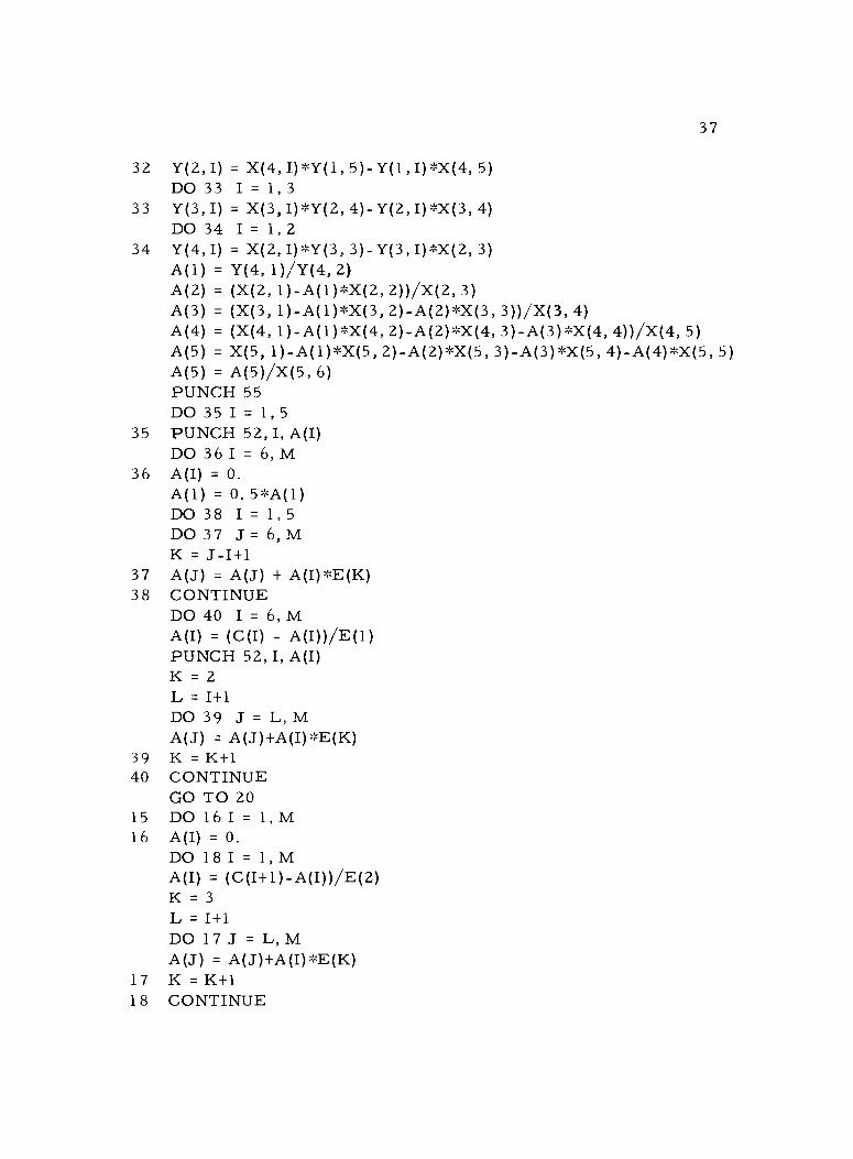
37
32 Y(2,I) = X(4, I)*Y(1, 5)-Y(1, I)mX(4, 5) DO 33 I = 1,3
33 Y(3, I) = X(3, I) *Y(2, 4)-Y(2, I) *X(3, 4) DO 34 I= 1,2
34 Y(4, I) = X(2, I)*Y(3, 3)-Y(3, I)mX(2, 3) A(1) = Y(4, 1)/Y(4, 2) A(2) = (X(2, 1)-A(1)*X(2, 2))/X(2, 3) A(3) = (X(3, 1)-A(1)mX(3, 2)-A(2)MX(3, 3))/X(3, 4) A(4) = (X(4, 1)-A(1)mX(4, 2)-A(2)mX(4, 3)-A(3)*X(4, 4))/X(4, 5) A(5) = X(5, 1)-A(1) *X(5, 2)-A(2)MX(5, 3)-A(3)*X(5, 4)-A(4)^X(5, A(5) = A(5)/X(5, 6) PUNCH 55 DO35I=1,5
35 PUNCH 52, I, A(I) DO 36 I = 6, M
36 A(I) = O.
A(1) = 0. 5*A(1) DO38I=1,5 DO 37 J = 6, M K = J-I+1
37 A(J) = A(J) + A(I)*E(K) 38 CONTINUE
D040 I= 6,M A(I) = (C(I) - A(I))/E(1) PUNCH 52, I, A(I) K =
L = I+1 D039 J=L,M A(J) = A(J)+A(I)*E(K)
39 K =K+1 40 CONTINUE
GO TO 20 15 DO16I=1,M 16 A(I) = 0.
DO 18I = 1, M A(I) = (C(I+1)-A(I))/E(2) K = 3
L = I+1 DO 17J =L,M A(J) = A(J)+A(I)*E(K)
17 K = K+1 18 CONTINUE
5)
2
38
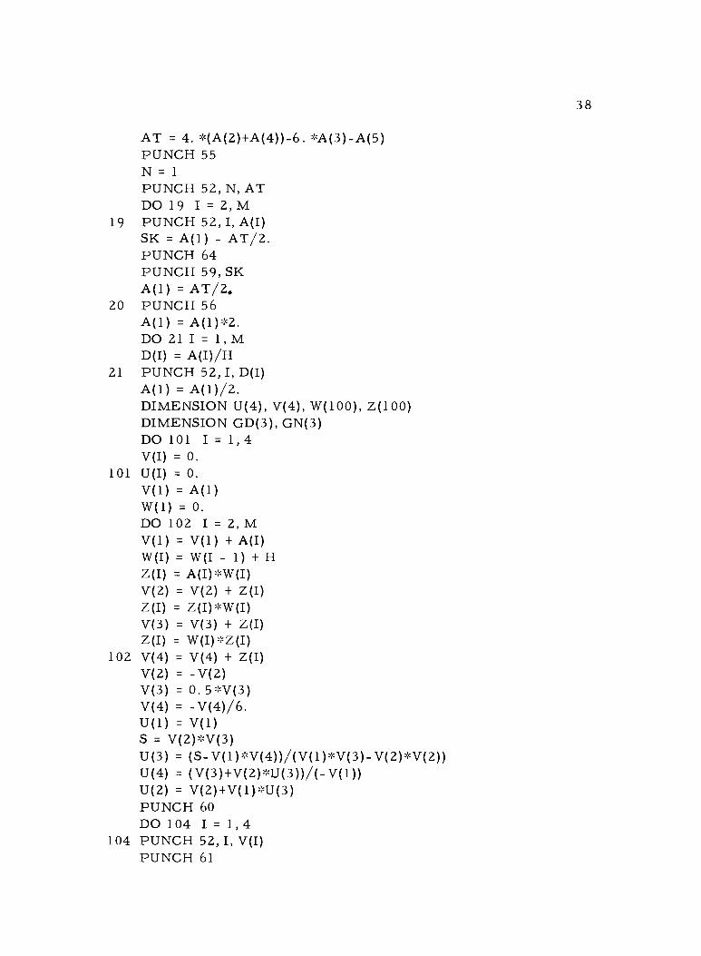
AT = 4. *(A(2)+A(4))-6. *A(3)-A(5) PUNCH 55 N = 1
PUNCH 52, N, AT DO 19 I = 2, M
19 PUNCH 52, I, A(I) SK = A(1) - AT/2. PUNCH 64 PUNCH 59, SK A(1) = AT/2
20 PUNCH 56 A(1) = A(1) *2. DO 21 I = 1,M D(I) = A(I)/H
21 PUNCH 52, I, D(I) A(1) = A(1)/2. DIMENSION U(4), V(4), W(100), Z(100) DIMENSION GD(3), GN(3) DO 101 I = 1,4 V(I) = O.
101 U(I) = O.
V(1) = A(1) W(1) = O.
DO 102 I = 2, M V(1) = V(1) + A(I) W(I) = W(I - 1) + H Z(I) = A(I)*W(I) V(2) = V(2) + Z(I) Z(I) = Z(I)*W(I) V(3) = V(3) + Z(I) Z(I) = W(I) *Z(I)
102 V(4) = V(4) + Z(I) V(2) = -V(2) V(3) = O. 5*V(3) V(4) = -V(4)/6. U(1) = V(1) S = V(2)*V(3) U(3) = (S-V(1)*V(4))/(V(1)*V(3)-V(2) er,V(2)) U(4) = ( V(3)+V(2)*U(3))/(- V(1)) U(2) = V(2)+V(1)*U(3) PUNCH 60 DO 104 I = 1,4
104 PUNCH 52, I, V(I) PUNCH 61
39
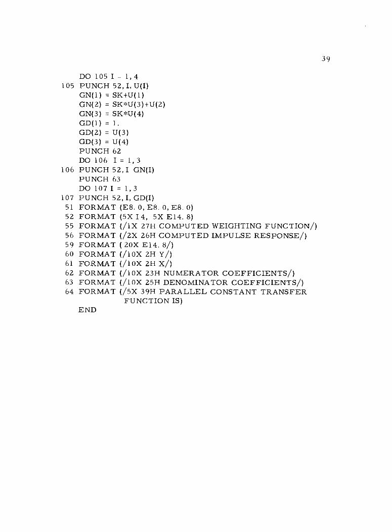
DO 105 I = 1, 4 105 PUNCH 52, I, U(I)
GN(1) = SK +U(1) GN(2) = SK *U(3) +U(2) GN(3) = SK *U(4) GD(1) = 1.
GD(2) = U(3) GD(3) = U(4) PUNCH 62 DO 106 I = 1,3
106 PUNCH 52,1 GN(I) PUNCH 63 DO 107 I = 1,3
107 PUNCH 52, I, GD(I) 51 FORMAT (E8. 0, E8. 0, E8. 0) 52 FORMAT (5X I4, 5X E14. 8) 55 FORMAT ( /1X 27H COMPUTED WEIGHTING FUNCTION) 56 FORMAT ( /2X 26H COMPUTED IMPULSE RESPONSE/) 59 FORMAT (20X E14. 8/) 60 FORMAT ( /10X 2H Y/) 61 FORMAT ( /10X 2H X/) 62 FORMAT ( /10X 23H NUMERATOR COEFFICIENTS /) 63 FORMAT ( /10X 25H DENOMINATOR COEFFICIENTS /) 64 FORMAT ( /5X 39H PARALLEL CONSTANT TRANSFER
FUNCTION IS) END
40
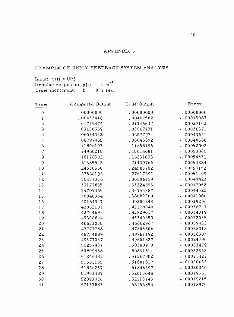
APPENDIX 5
EXAMPLE OF UNITY FEEDBACK SYSTEM ANALYSIS
Input: r(t) = U(t) Impulse response: g(t) = t e Time increment: h = 0.1 sec.
Time Computed Output True Output Error 0 00000000 00000000 .00000000 1 00452418 00467502 -.00015083 2 01719474 01746637 -.00027162 3 03630559 03667131 -.00036571 4 06034332 06077974 -.00043641 5 08797965 08846652 -.00048686 6 11806193 .11858195 -.00052002 7 14960215 .15014081 -.00053866 8 18176502 .18231033 -.00054531 9 21385542 .21439766 -.00054224
10 24530550 .24583702 -.00053152 11 27566192 .27617691 -.00051499 12 30457336 .30506759 -.00049423 13 33177835 .33224893 -.00047058 14 35709365 .35753887 -.00044522 15 38040354 .38082260 -.00041906 16 40164947 .40204243 -.00039296 17 42082101 .42118848 -.00036747 18 43794698 .43829017 -.00034319 19 45308824 .45340859 -.00032035 20 46633035 .46662967 -.00029932 21 47777788 .47805806 -.00028018 22 48754889 .48781192 -.00026303 23 49577037 .49601827 -.00024790 24 50257431 .50280910 -.00023479 25 50809456 .50831814 -.00022358 26 51246381 .51267802 -.00021421 27 51581165 .51601817 -.00020652 28 51826257 .51846297 -.00020040 29 51993487 .52013048 -.00019561 30 52093928 .52113143 -.00019215 31 52137883 .52156853 -.00018970
41
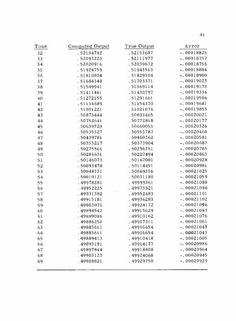
Time Computed Output True Output Error
32 .52134782 .52153607 -.00018825
33 .52093220 .52111977 -.00018757
34 .52020916 .52039672 -.00018756
35 . 51924759 . 51943563 -. 00018804
36 . 51810804 . 51829704 -. 00018900
37 . 51684348 . 51703371 -. 00019023
38 .51549941 .51569114 -.00019173
39 .51411461 .51430797 -.00019336
40 .51272155 .51291661 -.00019506
41 .51134689 .51154370 -.00019681
42 .51001221 .51021076 -.00019855
43 . 50873444 . 50893465 -.00020021
44 .50752641 .50772818 -.00020177
45 .50639729 .50660055 -.00020326
46 .50535327 .50555787 -.00020460
47 . 50439781 . 50460362 -.00020581
48 .50353217 .50373904 -.00020687
49 . 50275566 . 50296351 -.00020785
50 .50206631 .50227494 -.00020863
51 .50146073 .50167001 -.00020928
52 .50093470 .50114451 -.00020981
53 .50048331 .50069356 -.00021025
54 .50010121 .50031180 -.00021059
55 .49978281 _49999361 -. 00021080
56 .49952225 .49973321 -.00021096
57 .49931382 . 49952483 -.00021101
58 .49915181 .4993 6283 -.00021102
59 .49903076 .49924172 -.00021096
60 .49894542 .49915629 -.00021087
61 .49889086 .49910162 -.00021076
62 .49886250 .49907311 -.00021061
63 .49885611 .49906654 -.00021043
64 .49885611 .49906654 -.00021043
65 .49889413 .49910418 -.00021005
66 .49893191 .49914177 -.00020986
67 .49897844 .49918808 -.00020964
68 .49903123 .49924068 -.00020945
69 .49908821 .49929750 -.00020929
42
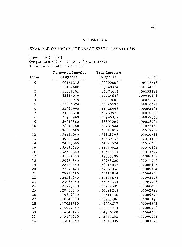
APPENDIX 6
EXAMPLE OF UNITY FEEDBACK SYSTEM SYNTHESIS
Input: r(t) = U(t) Output: c(t) = 0. 5 + 0. 707 e -t sin (t -3 n /r) Time increment: h = 0. 1 sec.
Computed Impulse Time Response
True Impulse Response Error
0 00168218 . 00000000 . 00168218 1 .09182608 .09048374 .00134233 2 .16488101 .16374614 .00133487 3 .22314089 .22224546 .00089543 4 26889979 26812801 .00077178 5 .30386574 .30326532 .00060042 6 .32981960 .32928698 .00053262 7 .34801640 .34760971 .00040669 8 .35983960 .35946317 .00037643 9 .36619360 .36591269 .00028091
10 .36815380 .36787944 .00027436 11 .36635680 .36615819 .00019861 12 .36164060 .36143305 .00020755 13 .35443620 .35429132 .00014488 14 .34539860 .34523574 .00016286 15 .33480380 .33469523 00010857 16 .32316660 .32303443 .00013217 17 31064500 31056199 .00008301 18 .29764840 .29763800 .00011040 19 .28424440 .28418037 .00006403 20 .27076420 .27067056 .00009364 21 .25720680 .25715849 .00004831 22 .24384740 .24376694 .00008046 23 .23063040 .23059534 .00003506 24 .21779200 .21772309 .00006891 25 .20523640 .20521249 .00002391 26 .19317000 .19311130 .00005870 27 .18146880 .18145488 00001392 28 .17031680 .17026817 00004863 29 .15957240 .15956734 00000506 30 .14940120 .14936120 00004000 31 .13965000 .13965252 00000252 32 .13046980 .13043905 00003075
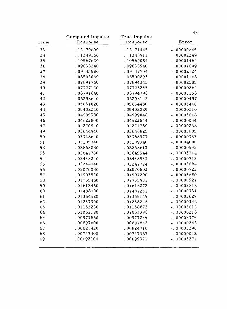
43
Time Computed Impulse
Response True Impulse Response Error
33 . 12170600 . 12171445 -. 00000845 34 .11349160 .11346911 .00002249 35 .10567620 .10569084 -.00001464 36 .09838240 .09836540 .00001699 37 .09145580 .09147704 -.00002124 38 .08502060 .08500893 .00001166 39 .07891760 .07894345 -.00002585 40 .07327120 .07326255 .00000864 41 .06791640 .06794796 -.00003156 42 .06298640 .06298142 .00000497 43 . 05831020 . 05834480 -. 00003460 44 .05402240 .05402029 .00000210 45 . 04995380 . 04999048 -.00003668
46 . 04623800 . 04523844 -. 00000044 47 .04270940 .04274780 -.00000238 49 . 03644940 . 03648825 -. 00003885
50 . 03368640 . 03368973 -. 00000333 51 . 03105340 . 03109340 -. 00004000 52 . 02868080 . 02868613 -. 00000533
53 . 02641780 . 02645544 -. 00003764 54 . 02438240 . 02438953 -. 00000713
55 .02244040 .02247724 -.00003684 56 . 02070080 . 02070803 -. 00000723 57 . 01903520 . 01907200 -. 00003680 58 . 01755460 . 01755981 -. 00000521
59 .01612460 .01616272 -.00003812 60 . 01486900 . 01487251 -. 00000351
61 . 01364520 . 01368149 -. 00003629 62 . 01257900 . 01258246 -. 00000346 63 .01153260 .01156872 -.00003612 64 . 01063180 . 01063396 -. 00000216 65 . 00973860 . 00977235 -. 00003375 66 . 00897600 . 00897842 -. 00000242 67 . 00821420 . 00824710 -. 00003290 68 .00757400 .00757367 .00000032 69 .00692100 .00695371 -.00003271