Hansjörg Geiges Christiaan Huygens and Contact Geometry NAW 5/6 nr. 2 juni 2005 117

Hansjörg GeigesMathematisches Institut

Universität zu Köln

Weyertal 86–90

50931 Köln

Duitsland

geiges@math.uni-koeln.de

Christiaan Huygens and Contact Geometry

In de tweede helft van de zeventiende eeuw formuleerden Pierre Fer-mat en Christiaan Huygens hun theorieën over de optica. Uitgangspuntvoor Fermat was het gegeven dat een lichtstraal de snelste weg zoekt,en voor Huygens dat elk punt van een golffront opgevat kan worden alseen nieuwe lichtbron. Hansjörg Geiges illustreert de beginselen vande contactmeetkunde aan de hand van deze zogenaamde principesvan Fermat en Huygens en laat met behulp van deze theorie zien datde twee principes equivalent zijn.

De tekst is gebaseerd op de inaugurele rede die Hansjörg Geigesop 24 januari 2003 uitsprak bij de aanvaarding van het ambt vanhoogleraar aan de Universität zu Köln. Daarvoor was hij hoogleraarmeetkunde aan de Universiteit Leiden.

“ —Oui, voilà le géomètre! Et ne crois pas que les géomètres n’aientpas à s’occuper des femmes!” (Jean Giraudoux, La guerre de Troien’aura pas lieu)

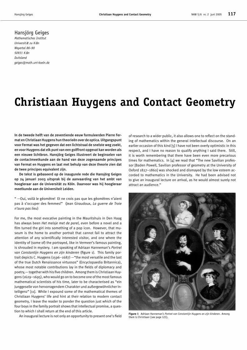
For me, the most evocative painting in the Mauritshuis in Den Haaghas always been Het meisje met de parel, even before a novel and afilm turned the girl into something of a pop icon. However, that mu-seum is the home to another portrait that cannot fail to attract theattention of any scientifically interested visitor, and one where theidentity of (some of) the portrayed, like in Vermeer’s famous painting,is shrouded in mystery. I am speaking of Adriaan Hanneman’s Portretvan Constantijn Huygens en zijn kinderen (figure 1). This family por-trait depicts C. Huygens (1596–1687) —“the most versatile and the lastof the true Dutch Renaissance virtuosos” (Encyclopaedia Britannica),whose most notable contributions lay in the fields of diplomacy andpoetry,— together with his five children. Among them is Christiaan Huy-gens (1629–1695), who would go on to become one of the most famousmathematical scientists of his time, later to be characterised as “einJunggeselle von hervorragendem Charakter und außergewöhnlicher In-telligenz” [11]. While I expound some of the mathematical themes ofChristiaan Huygens’ life and hint at their relation to modern contactgeometry, I leave the reader to ponder the question just which of thefour boys in the family portrait shows that intellectual promise, a ques-tion to which I shall return at the end of this article.

An inaugural lecture is not only an opportunity to present one’s field

of research to a wider public, it also allows one to reflect on the stand-ing of mathematics within the general intellectual discourse. On anearlier occasion of this kind [5] I have not been overly optimistic in thisrespect, and I have no reason to qualify anything I said there. Still,it is worth remembering that there have been even more precarioustimes for mathematics. In [4] we read that “The new Savilian profes-sor [Baden Powell, Savilian professor of geometry at the University ofOxford 1827–1860] was shocked and dismayed by the low esteem ac-corded to mathematics in the University. He had been advised notto give an inaugural lecture on arrival, as he would almost surely notattract an audience.”

Figure 1 Adriaan Hanneman’s Portret van Constantijn Huygens en zijn kinderen. Amongthem is Christiaan (see page 123).

118 NAW 5/6 nr. 2 juni 2005 Christiaan Huygens and Contact Geometry Hansjörg Geiges

DisclaimerA foreigner, even one who has lived in the Netherlands for several years,is obviously carrying tulips to Amsterdam (or whatever the appropriateturn of phrase might be) when writing about Christiaan Huygens in aDutch journal. Then again, from a visit to the Huygensmuseum Hofwijckin Voorburg near Den Haag I gathered that in the Netherlands the fameof Constantijn Huygens tends to outshine that of his second-eldest son.Be that as it may, this article is intended merely as a relatively faithfulrecord of my inaugural lecture (with some mathematical details added)and entirely devoid of scholarly aspirations.

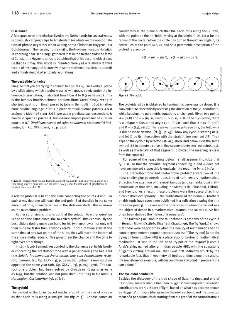
The best slide for twinsImagine that you are trying to connect two pointsA,B in a vertical planeby a slide along which a point mass M will move, solely under the in-fluence of gravitation, in shortest time from A to B (see figure 2). Thisis the famous brachistochrone problem (from Greek βραχιστoς =shortest, χρoνoς = time), posed by Johann Bernoulli in 1696 in rathermore erudite language: “Datis in plano verticali duobus punctis A & Bassignare Mobili M viam AMB, per quam gravitate sua descendens &moveri incipiens a punctoA, brevissimo tempore perveniat ad alterumpunctum B.” (Problema novum ad cujus solutionem Mathematici invi-tantur, Joh. Op. XXX (pars), [3], p. 212).

Figure 2 Imagine that you are trying to connect two points A,B in a vertical plane by aslide along which a point massM will move, solely under the influence of gravitation, inshortest time from A to B.

A related problem is to find the slide connecting the points A and B insuch a way that one will reach the end-point B of the slide in the sameamount of time, no matter where on the slide one starts. This is knownas the tautochrone problem.

Rather surprisingly, it turns out that the solution to either questionis one and the same curve, the so-called cycloid. This is obviously thebest slide a doting uncle can build for his twin nephews: not only willtheir slide be faster than anybody else’s; if both of them start at thesame time at any two points of the slide, they will reach the bottom ofthe slide simultaneously. This gives them the chance and the time tofight over other things.

In 1697 Jacob Bernoulli responded to the challenge set by his broth-er concerning the brachistochrone with a paper bearing the beautifultitle Solutio Problematum Fraternorum, una cum Propositione recip-roca aliorum, Jac. Op. LXXV ([3], p. 271–282). Johann’s own solutionappeared the same year (Joh. Op. XXXVII, [3], p. 263–270). The tau-tochrone problem had been solved by Christiaan Huygens as earlyas 1657, but the solution was not published until 1673 in his famousHorologium Oscillatorium [9], cf. [16].

The cycloidThe cycloid is the locus traced out by a point on the rim of a circleas that circle rolls along a straight line (figure 3). Choose cartesian

coordinates in the plane such that the circle rolls along the x–axis,with the point on the rim initially lying at the origin (0,0). Let a be theradius of the circle. When the circle has turned through an angle t, itscentre lies at the point (at,a), and so a parametric description of thecycloid is given by

x(t) = a(t − sin t), y(t) = a(1− cos t).

http

://m

athw

orld

.wol

fram

.com

Figure 3 The cycloid

The cycloidal slide is obtained by turning this curve upside down. It isconvenient to effect this by reversing the direction of they–coordinate,while keeping the parametric equations unchanged. Given two pointsA = (0,0) and B = (b1, b2) with b1 > 0, b2 ≥ 0 in the xy–plane, thereis a unique radius a and angle tB ∈ (0,2π ] such that A = (x(0), y(0))

and B = (x(tB ), y(tB )). There are various ways to see this, the followingis due to Isaac Newton, (cf. [3], p. 43): Draw any cycloid starting at A,and let Q be its intersection with the straight line segment AB. Thenexpand the cycloid by a factorAB/AQ. (Here and below I use the samesymbolAB to denote a curve or line segment between two pointsA,B,as well as the length of that segment, provided the meaning is clearfrom the context.)

For some of the reasonings below I shall assume implicitly thattB ≤ π , so that the cycloidal segment connecting A and B does nothave any upward slope; this is equivalent to requiring b2 ≥ 2b1/π .

The brachistochrone and tautochrone problems were two of themost challenging geometric questions of 17th century mathematics,attracting the attention of the most famous (and cantankerous) math-ematicians of that time, including the Marquis de L’Hospital, Leibniz,and Newton. As a result, these problems were the source of acrimo-nious battles over priority — the publications of the Bernoulli brotherson this topic have even been published in a collection bearing the titleStreitschriften [3]. This was not the only occasion when the cycloid wasthe object of desire in a mathematical quarrel, and so this curve hasoften been dubbed the ‘Helen of Geometers’.

The following allusion to the tautochronous property of the cycloidin Herman Melville’s Moby Dick ([13], Chapter 96, The Try-Works) showsthat there were happy times when the beauty of mathematics had tosome degree entered popular consciousness: “[The try-pot] [a pot fortrying oil from blubber -HG] is a place also for profound mathematicalmeditation. It was in the left hand try-pot of the Pequod [CaptainAhab’s ship, named after an Indian people -HG], with the soapstonediligently circling around me, that I was first indirectly struck by theremarkable fact, that in geometry all bodies gliding along the cycloid,my soapstone for example, will descend from any point in precisely thesame time.”

The cycloidal pendulumBesides the discovery of the true shape of Saturn’s rings and one ofits moons, namely Titan, Christiaan Huygens’ most important scientificcontributions are his theory of light, based on what has become knownas Huygens’ principle (discussed in the next section), and his develop-ment of a pendulum clock starting from his proof of the tautochronous

Hansjörg Geiges Christiaan Huygens and Contact Geometry NAW 5/6 nr. 2 juni 2005 119

property of the cycloid.At the time of Huygens, pendulum clocks were built (as they usually

are today) with a simple circular pendulum. The problem with such apendulum is that its frequency depends on the amplitude of the oscil-lation. With regard to the pendulum clock in your living room this is nocause for concern, since there the amplitude stays practically constant.But arguably the most outstanding problem of applied mathematics atthat time was to build a clock that was also reliable in more adverseconditions, say on a ship sailing through gale force winds. Why aresuch accurate clocks important?

As is wryly remarked in the introduction to the lavishly illustratedproceedings of the Longitude Symposium [2], “Travelling overseas, wenow complain when delayed for an hour: we have forgotten that oncethere were problems finding continents”. Indeed, how was it possibleto determine your exact position at sea (or anywhere else, for thatmatter), prior to the days of satellite-based Global Positioning Systems?Mathematically the answer is simple (at least on a sunny day): Observewhen the sun reaches its highest elevation. This will be noon local time.Moreover, the angleα of elevation will give you the latitude: If the axisof the earth’s rotation were orthogonal to the plane in which the earthmoves around the sun, that latitude would simply be 90◦ −α. In orderto take the tilting of the earth’s axis by 23◦ into account, one needs toadjust this by an angle that depends on the date, varying between 0◦

at the equinoxes and ±23◦ at the solstices.The longitude, on the other hand, cannot be determined from this

observational data alone. Indeed, the actual value of the longitudeat any given point is a matter of convention. The fact that the zeromeridian passes through Greenwich is a consequence of the scientificachievements and geopolitical power of the British, not astronomy.However, if you keep a clock with you that shows accurate Greenwichtime, and you bear in mind that the earth rotates by a full 360◦ in 24hours, then multiplying the difference between your local time and thatshown on the clock by 15◦/h will determine your longitude relative tothat of Greenwich.

All the practical problems involved in building such an accurateclock were first solved by John Harrison in 1759: cf. [2] and the thrillingaccount of Harrison’s life in [14].

From a mathematical point of view, the question addressed by Huy-gens concerned the most interesting aspect of these practical prob-lems: Is it possible to devise a pendulum whose frequency does notdepend on the amplitude of the pendular motion? The hardest partof this question is to find the tautochronous curve, along which thependulum mass should be forced to move. This Huygens establishedto be the cycloid. He further observed that one could make the pen-dulum move along a cycloid by restricting the swinging motion of thependulum between appropriately shaped plates.

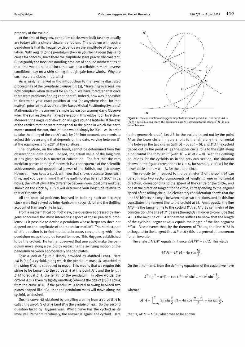
Take a look at figure 4 (kindly provided by Manfred Lehn). HereAB is (half) a cycloid, along which the pendulum massM, attached tothe string B′M, is supposed to move. This means that we require thisstring to be tangent to the curve B′A at the point M′, and the lengthB′M to equal B′A, the length of the pendulum. In other words, thecycloidAB is given by tightly unrolling (whence the title of [16]) a stringfrom the curve B′A. If the pendulum is forced to swing between twoplates shaped like B′A, then the pendulum mass will move along thecycloid, as desired.

Such a curve AB obtained by unrolling a string from a curve B′A iscalled the involute of B′A (and B′A the evolute of AB). So the secondquestion faced by Huygens was: Which curve has the cycloid as itsinvolute? Rather miraculously, the answer is again: the cycloid. Here

Figure 4 The construction of Huygens amplitude invariant pendulum. The curve AB is(half) a cycloid, along which the pendulum massM , attached to the string B′M , is sup-posed to move.

is the geometric proof: Let AB be the cycloid traced out by the pointM as the lower circle in figure 4 rolls to the left along the horizontalline between the two circles (withM = A at t = 0), and B′A the cycloidtraced out by the point M′ as the upper circle rolls to the right alonga horizontal line through B′ (with M′ = B′ at t = 0). With the definingequations for the cycloids as in the previous section, the situationshown in the figure corresponds to t = t0 for some t0 ∈ [0, π ] for thelower circle and t = π − t0 for the upper circle.

The velocity (with respect to the parameter t) of the point M canbe split into two vector components of length a: one in horizontaldirection, corresponding to the speed of the centre of the circle, andone in the direction tangent to the circle, corresponding to the angularspeed of the rolling circle. An elementary consideration shows that thelineMP bisects the angle between these two directions, and so this lineconstitutes the tangent line to the cycloid at M. Analogously, the lineM′P ′ is the tangent line to the cycloid B′A at M′. By symmetry of theconstruction, the lineM′P ′ passes throughM. In order to conclude thatAB is the involute of B′A it therefore suffices to show that the lengthof the cycloidal segment M′A equals the length of the line segmentM′M. Also observe that, by the theorem of Thales, the line M′M isorthogonal to the tangent lineMP atM ; this is a general phenomenonfor an involute.

The angle ∠MOP ′ equals t0, hence ∠MPP ′ = t0/2. This yields

M′M = 2P ′M = 4a sint02.

On the other hand, from the defining equations of the cycloid we have

x2 + y2 = a2(1− cos t)2 + a2 sin2 t = 4a2 sin2 t2,

whence

M′A =∫ ππ−t0

2a sint2dt = 4a cos

π − t02

= 4a sint02,

that is,M′M = M′A, which was to be shown.

120 NAW 5/6 nr. 2 juni 2005 Christiaan Huygens and Contact Geometry Hansjörg Geiges

Figure 5 The construction plan from Huygens’ Horologium Oscillatorium , with the cycloidalplates indicated by ‘FIG. II’

Huygens did not stop at these theoretical considerations, but proceed-ed to construct an actual pendulum clock with cycloidal plates. Theconstruction plan from Huygens’ Horologium Oscillatorium, with thecycloidal plates indicated by ‘FIG. II’, is shown in figure 5. A replica ofthis clock can be seen in the Huygensmuseum Hofwijck.

Geometric opticsEither of the following fundamental principles can be used to explainthe propagation of light:

Fermat’s Principle (1658). Any ray of light follows the path of shortesttime.

Huygens’ Principle (1690). Every point of a wave front is the source ofan elementary wave. The wave front at a later time is given as theenvelope of these elementary waves [10].

Figure 6 Fermat’s principle versus Huygens’ principle

The simplest possible example is the propagation of light in a homo-geneous and isotropic medium. Here we expect the rays of light tobe straight lines. Figure 6 illustrates that this is indeed what the twoprinciples predict. We merely need to observe that, in a homogeneousand isotropic medium, the curves of shortest time are the same as geo-metrically shortest curves, i.e. straight lines, and elementary waves arecircular waves around their centre.

Whereas Fermat’s principle can only be justified as an instance ofnature’s parsimony, cf. [8], Huygens’ principle can be explained mech-anistically from a particle theory of light, see figure 7.

Figure 7 Explanation of Huygens’ principle from the particle theory of light

To illustrate the power of these principles, here are two further exam-ples. The first is the law of reflection, which states that the angle ofincidence equals the angle of reflection. Figure 8 shows how this fol-lows from Fermat’s principle: The path connecting A and B has thesame length as the corresponding one connecting A and the mirrorimage B′ of B, and for the latter the shortest (and hence quickest) pathis given by the straight line.

Figure 8 The law of reflection, by the Fermat principle

The explanation of the law of reflection from Huygens’ principle is il-lustrated in figure 9.

Figure 9 The law of reflection, by the Huygens principle

As a final application of the two principles, we turn to the law of refrac-tion, also known as Snell’s law after the Dutch astronomer and math-ematician Willebrord van Roijen Snell (1580–1628), whose latinisedname Snellius now adorns the Mathematical Institute of the Univer-siteit Leiden. Snell discovered this law in 1621; in print it appears forinstance in Huygens’ Traité de la lumière, with proofs based on eitherof the two principles. The law states that as a ray of light crosses theboundary between two (homogeneous and isotropic) optical media,the angle of incidenceα1 (measured relative to a line perpendicular tothe separating surface) and the angle of refraction α2 (see figure 10)are related by

Hansjörg Geiges Christiaan Huygens and Contact Geometry NAW 5/6 nr. 2 juni 2005 121

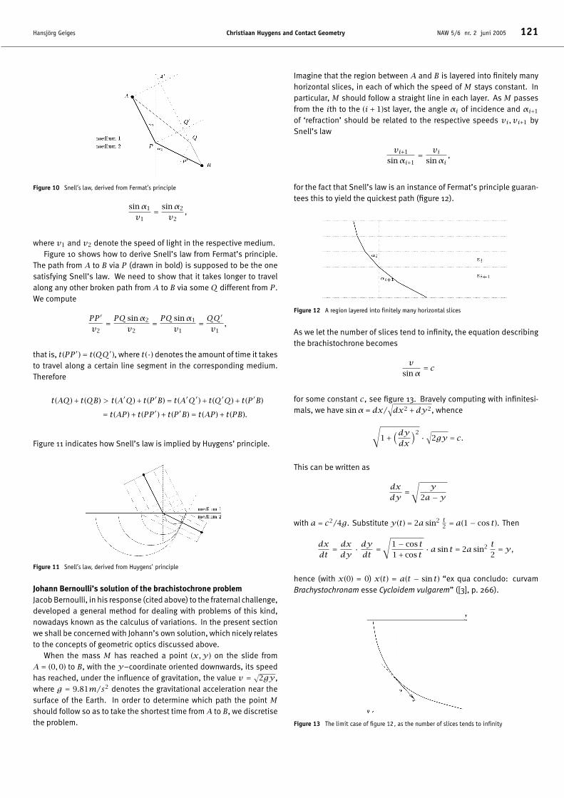
Figure 10 Snell’s law, derived from Fermat’s principle

sinα1

v1=

sinα2

v2,

where v1 and v2 denote the speed of light in the respective medium.Figure 10 shows how to derive Snell’s law from Fermat’s principle.

The path from A to B via P (drawn in bold) is supposed to be the onesatisfying Snell’s law. We need to show that it takes longer to travelalong any other broken path from A to B via some Q different from P .We compute

PP ′

v2=PQ sinα2

v2=PQ sinα1

v1=QQ′

v1,

that is, t(PP ′) = t(QQ′), where t(·) denotes the amount of time it takesto travel along a certain line segment in the corresponding medium.Therefore

t(AQ) + t(QB) > t(A′Q) + t(P ′B) = t(A′Q′) + t(Q′Q) + t(P ′B)

= t(AP ) + t(PP ′) + t(P ′B) = t(AP ) + t(PB).

Figure 11 indicates how Snell’s law is implied by Huygens’ principle.

Figure 11 Snell’s law, derived from Huygens’ principle

Johann Bernoulli’s solution of the brachistochrone problemJacob Bernoulli, in his response (cited above) to the fraternal challenge,developed a general method for dealing with problems of this kind,nowadays known as the calculus of variations. In the present sectionwe shall be concerned with Johann’s own solution, which nicely relatesto the concepts of geometric optics discussed above.

When the mass M has reached a point (x,y) on the slide fromA = (0,0) to B, with the y–coordinate oriented downwards, its speedhas reached, under the influence of gravitation, the value v =

√2gy,

where g = 9.81m/s2 denotes the gravitational acceleration near thesurface of the Earth. In order to determine which path the point Mshould follow so as to take the shortest time fromA to B, we discretisethe problem.

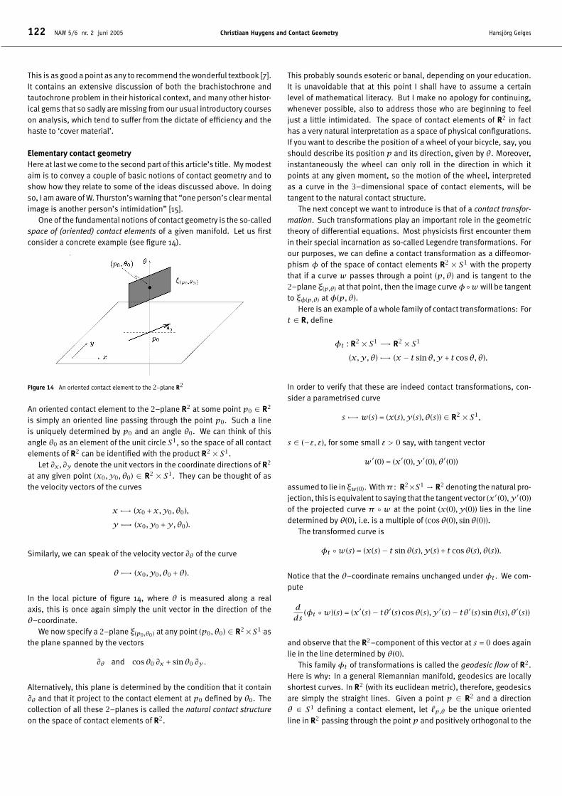
Imagine that the region between A and B is layered into finitely manyhorizontal slices, in each of which the speed of M stays constant. Inparticular, M should follow a straight line in each layer. As M passesfrom the ith to the (i + 1)st layer, the angle αi of incidence and αi+1

of ‘refraction’ should be related to the respective speeds vi, vi+1 bySnell’s law

vi+1

sinαi+1=

visinαi

,

for the fact that Snell’s law is an instance of Fermat’s principle guaran-tees this to yield the quickest path (figure 12).

Figure 12 A region layered into finitely many horizontal slices

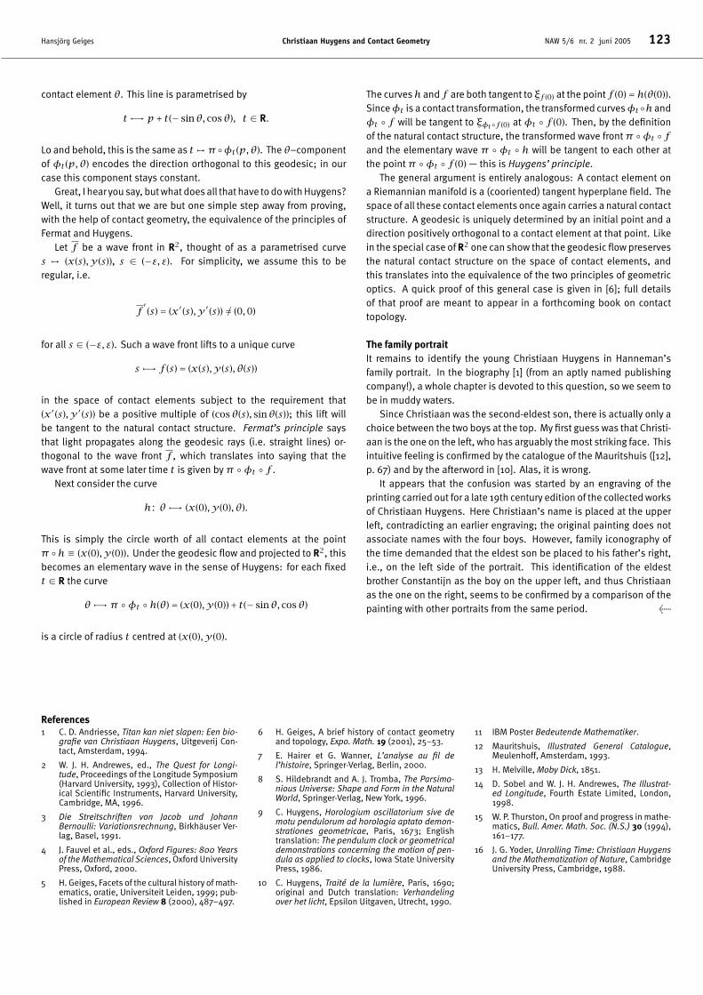
As we let the number of slices tend to infinity, the equation describingthe brachistochrone becomes

vsinα

= c

for some constant c, see figure 13. Bravely computing with infinitesi-mals, we have sinα = dx/

√dx2 + dy2, whence

√1 +

(dydx

)2·√

2gy = c.

This can be written as

dxdy

=

√y

2a−y

with a = c2/4g. Substitute y(t) = 2a sin2 t2 = a(1− cos t). Then

dxdt

=dxdy

· dydt

=

√1− cos t1 + cos t

· a sin t = 2a sin2 t2

= y,

hence (with x(0) = 0) x(t) = a(t − sin t) “ex qua concludo: curvamBrachystochronam esse Cycloidem vulgarem” ([3], p. 266).

Figure 13 The limit case of figure 12, as the number of slices tends to infinity

122 NAW 5/6 nr. 2 juni 2005 Christiaan Huygens and Contact Geometry Hansjörg Geiges

This is as good a point as any to recommend the wonderful textbook [7].It contains an extensive discussion of both the brachistochrone andtautochrone problem in their historical context, and many other histor-ical gems that so sadly are missing from our usual introductory courseson analysis, which tend to suffer from the dictate of efficiency and thehaste to ‘cover material’.

Elementary contact geometryHere at last we come to the second part of this article’s title. My modestaim is to convey a couple of basic notions of contact geometry and toshow how they relate to some of the ideas discussed above. In doingso, I am aware of W. Thurston’s warning that “one person’s clear mentalimage is another person’s intimidation” [15].

One of the fundamental notions of contact geometry is the so-calledspace of (oriented) contact elements of a given manifold. Let us firstconsider a concrete example (see figure 14).

Figure 14 An oriented contact element to the 2–plane R2

An oriented contact element to the 2–plane R2 at some point p0 ∈ R2

is simply an oriented line passing through the point p0. Such a lineis uniquely determined by p0 and an angle θ0. We can think of thisangle θ0 as an element of the unit circle S1, so the space of all contactelements of R2 can be identified with the product R2 × S1.

Let ∂x , ∂y denote the unit vectors in the coordinate directions of R2

at any given point (x0, y0, θ0) ∈ R2 × S1. They can be thought of asthe velocity vectors of the curves

x 7−→ (x0 + x,y0, θ0),

y 7−→ (x0, y0 +y,θ0).

Similarly, we can speak of the velocity vector ∂θ of the curve

θ 7−→ (x0, y0, θ0 + θ).

In the local picture of figure 14, where θ is measured along a realaxis, this is once again simply the unit vector in the direction of theθ–coordinate.

We now specify a 2–plane ξ(p0,θ0) at any point (p0, θ0) ∈ R2×S1 asthe plane spanned by the vectors

∂θ and cosθ0 ∂x + sinθ0 ∂y .

Alternatively, this plane is determined by the condition that it contain∂θ and that it project to the contact element at p0 defined by θ0. Thecollection of all these 2–planes is called the natural contact structureon the space of contact elements of R2.

This probably sounds esoteric or banal, depending on your education.It is unavoidable that at this point I shall have to assume a certainlevel of mathematical literacy. But I make no apology for continuing,whenever possible, also to address those who are beginning to feeljust a little intimidated. The space of contact elements of R2 in facthas a very natural interpretation as a space of physical configurations.If you want to describe the position of a wheel of your bicycle, say, youshould describe its position p and its direction, given by θ. Moreover,instantaneously the wheel can only roll in the direction in which itpoints at any given moment, so the motion of the wheel, interpretedas a curve in the 3–dimensional space of contact elements, will betangent to the natural contact structure.

The next concept we want to introduce is that of a contact transfor-mation. Such transformations play an important role in the geometrictheory of differential equations. Most physicists first encounter themin their special incarnation as so-called Legendre transformations. Forour purposes, we can define a contact transformation as a diffeomor-phism φ of the space of contact elements R2 × S1 with the propertythat if a curve w passes through a point (p,θ) and is tangent to the2–plane ξ(p,θ) at that point, then the image curveφ◦w will be tangentto ξφ(p,θ) atφ(p,θ).

Here is an example of a whole family of contact transformations: Fort ∈ R, define

φt : R2 × S1 −→ R2 × S1

(x,y,θ) 7−→ (x − t sinθ,y + t cosθ,θ).

In order to verify that these are indeed contact transformations, con-sider a parametrised curve

s 7−→ w(s) = (x(s), y(s), θ(s)) ∈ R2 × S1,

s ∈ (−ε, ε), for some small ε > 0 say, with tangent vector

w′(0) = (x′(0), y′(0), θ′(0))

assumed to lie inξw(0). Withπ : R2×S1 → R2 denoting the natural pro-jection, this is equivalent to saying that the tangent vector (x′(0), y′(0))

of the projected curve π ◦ w at the point (x(0), y(0)) lies in the linedetermined by θ(0), i.e. is a multiple of (cosθ(0), sinθ(0)).

The transformed curve is

φt ◦w(s) = (x(s)− t sinθ(s), y(s) + t cosθ(s), θ(s)).

Notice that the θ–coordinate remains unchanged under φt . We com-pute

dds

(φt ◦w)(s) = (x′(s)− tθ′(s) cosθ(s), y′(s)− tθ′(s) sinθ(s), θ′(s))

and observe that the R2–component of this vector at s = 0 does againlie in the line determined by θ(0).

This family φt of transformations is called the geodesic flow of R2.Here is why: In a general Riemannian manifold, geodesics are locallyshortest curves. In R2 (with its euclidean metric), therefore, geodesicsare simply the straight lines. Given a point p ∈ R2 and a directionθ ∈ S1 defining a contact element, let `p,θ be the unique orientedline in R2 passing through the point p and positively orthogonal to the

Hansjörg Geiges Christiaan Huygens and Contact Geometry NAW 5/6 nr. 2 juni 2005 123

contact element θ. This line is parametrised by

t 7−→ p + t(− sinθ, cosθ), t ∈ R.

Lo and behold, this is the same as t 7→ π ◦φt (p,θ). The θ–componentof φt (p,θ) encodes the direction orthogonal to this geodesic; in ourcase this component stays constant.

Great, I hear you say, but what does all that have to do with Huygens?Well, it turns out that we are but one simple step away from proving,with the help of contact geometry, the equivalence of the principles ofFermat and Huygens.

Let f be a wave front in R2, thought of as a parametrised curves 7→ (x(s), y(s)), s ∈ (−ε, ε). For simplicity, we assume this to beregular, i.e.

f′(s) = (x′(s), y′(s)) 6= (0,0)

for all s ∈ (−ε, ε). Such a wave front lifts to a unique curve

s 7−→ f (s) = (x(s), y(s), θ(s))

in the space of contact elements subject to the requirement that(x′(s), y′(s)) be a positive multiple of (cosθ(s), sinθ(s)); this lift willbe tangent to the natural contact structure. Fermat’s principle saysthat light propagates along the geodesic rays (i.e. straight lines) or-thogonal to the wave front f , which translates into saying that thewave front at some later time t is given by π ◦φt ◦ f .

Next consider the curve

h : θ 7−→ (x(0), y(0), θ).

This is simply the circle worth of all contact elements at the pointπ ◦h ≡ (x(0), y(0)). Under the geodesic flow and projected to R2, thisbecomes an elementary wave in the sense of Huygens: for each fixedt ∈ R the curve

θ 7−→ π ◦φt ◦ h(θ) = (x(0), y(0)) + t(− sinθ, cosθ)

is a circle of radius t centred at (x(0), y(0).

The curvesh and f are both tangent to ξf (0) at the point f (0) = h(θ(0)).Sinceφt is a contact transformation, the transformed curvesφt◦h andφt ◦ f will be tangent to ξφt◦f (0) at φt ◦ f (0). Then, by the definitionof the natural contact structure, the transformed wave front π ◦φt ◦ fand the elementary wave π ◦φt ◦ h will be tangent to each other atthe point π ◦φt ◦ f (0) — this is Huygens’ principle.

The general argument is entirely analogous: A contact element ona Riemannian manifold is a (cooriented) tangent hyperplane field. Thespace of all these contact elements once again carries a natural contactstructure. A geodesic is uniquely determined by an initial point and adirection positively orthogonal to a contact element at that point. Likein the special case of R2 one can show that the geodesic flow preservesthe natural contact structure on the space of contact elements, andthis translates into the equivalence of the two principles of geometricoptics. A quick proof of this general case is given in [6]; full detailsof that proof are meant to appear in a forthcoming book on contacttopology.

The family portraitIt remains to identify the young Christiaan Huygens in Hanneman’sfamily portrait. In the biography [1] (from an aptly named publishingcompany!), a whole chapter is devoted to this question, so we seem tobe in muddy waters.

Since Christiaan was the second-eldest son, there is actually only achoice between the two boys at the top. My first guess was that Christi-aan is the one on the left, who has arguably the most striking face. Thisintuitive feeling is confirmed by the catalogue of the Mauritshuis ([12],p. 67) and by the afterword in [10]. Alas, it is wrong.

It appears that the confusion was started by an engraving of theprinting carried out for a late 19th century edition of the collected worksof Christiaan Huygens. Here Christiaan’s name is placed at the upperleft, contradicting an earlier engraving; the original painting does notassociate names with the four boys. However, family iconography ofthe time demanded that the eldest son be placed to his father’s right,i.e., on the left side of the portrait. This identification of the eldestbrother Constantijn as the boy on the upper left, and thus Christiaanas the one on the right, seems to be confirmed by a comparison of thepainting with other portraits from the same period. k

References1 C. D. Andriesse, Titan kan niet slapen: Een bio-

grafie van Christiaan Huygens, Uitgeverij Con-tact, Amsterdam, 1994.

2 W. J. H. Andrewes, ed., The Quest for Longi-tude, Proceedings of the Longitude Symposium(Harvard University, 1993), Collection of Histor-ical Scientific Instruments, Harvard University,Cambridge, MA, 1996.

3 Die Streitschriften von Jacob und JohannBernoulli: Variationsrechnung, Birkhäuser Ver-lag, Basel, 1991.

4 J. Fauvel et al., eds., Oxford Figures: 800 Yearsof the Mathematical Sciences, Oxford UniversityPress, Oxford, 2000.

5 H. Geiges, Facets of the cultural history of math-ematics, oratie, Universiteit Leiden, 1999; pub-lished in European Review 8 (2000), 487–497.

6 H. Geiges, A brief history of contact geometryand topology, Expo. Math. 19 (2001), 25–53.

7 E. Hairer et G. Wanner, L’analyse au fil del’histoire, Springer-Verlag, Berlin, 2000.

8 S. Hildebrandt and A. J. Tromba, The Parsimo-nious Universe: Shape and Form in the NaturalWorld, Springer-Verlag, New York, 1996.

9 C. Huygens, Horologium oscillatorium sive demotu pendulorum ad horologia aptato demon-strationes geometricae, Paris, 1673; Englishtranslation: The pendulum clock or geometricaldemonstrations concerning the motion of pen-dula as applied to clocks, Iowa State UniversityPress, 1986.

10 C. Huygens, Traité de la lumière, Paris, 1690;original and Dutch translation: Verhandelingover het licht, Epsilon Uitgaven, Utrecht, 1990.

11 IBM Poster Bedeutende Mathematiker.

12 Mauritshuis, Illustrated General Catalogue,Meulenhoff, Amsterdam, 1993.

13 H. Melville, Moby Dick, 1851.

14 D. Sobel and W. J. H. Andrewes, The Illustrat-ed Longitude, Fourth Estate Limited, London,1998.

15 W. P. Thurston, On proof and progress in mathe-matics, Bull. Amer. Math. Soc. (N.S.) 30 (1994),161–177.

16 J. G. Yoder, Unrolling Time: Christiaan Huygensand the Mathematization of Nature, CambridgeUniversity Press, Cambridge, 1988.